Action-Conditioned 3D Human Motion Synthesis with Transformer VAE

Abstract

We tackle the problem of action-conditioned generation of realistic and diverse human motion sequences. In contrast to methods that complete, or extend, motion sequences, this task does not require an initial pose or sequence. Here we learn an action-aware latent representation for human motions by training a generative variational autoencoder (VAE). By sampling from this latent space and querying a certain duration through a series of positional encodings, we synthesize variable-length motion sequences conditioned on a categorical action. Specifically, we design a Transformer-based architecture, ACTOR, for encoding and decoding a sequence of parametric SMPL human body models estimated from action recognition datasets. We evaluate our approach on the NTU RGB+D, HumanAct12 and UESTC datasets and show improvements over the state of the art. Furthermore, we present two use cases: improving action recognition through adding our synthesized data to training, and motion denoising. Code and models are available on our project page [57].

1 Introduction

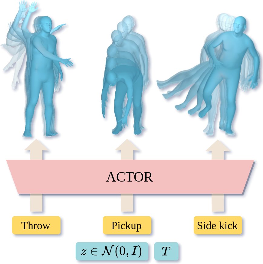
Fig. 1: Goal: Action-Conditioned TransfORmer VAE (ACTOR) learns to synthesize human motion sequences conditioned on a categorical action and a duration, $T$. Sequences are generated by sampling from a single motion representation latent vector, $z$, as opposed to the frame-level embedding space in prior work.

Despite decades of research on modeling human motions [4, 5], synthesizing realistic and controllable sequences remains extremely challenging. In this work, our goal is to take a semantic action label like “Throw” and generate an infinite number of realistic 3D human motion sequences, of varying length, that look like realistic throwing (Figure 1). A significant amount of prior work has focused on taking one pose, or a sequence of poses, and then predicting future motions [22, 6, 3, 74, 71]. This is an overly constrained scenario because it assumes that one already has a motion sequence and just needs more of it. On the other hand, many applications such as virtual reality and character control [28, 61] require generating motions of a given type (semantic action label) with a specified duration.

We address this problem by training an action-conditioned generative model with 3D human motion data that has corresponding action labels. In particular, we construct a Transformer-based encoder-decoder architecture and train it with the VAE objective. We parameterize the human body using SMPL [46] as it can output joint locations or the body surface. This paves the way for better modeling of interaction with the environment, as the surface is necessary to model contact. Moreover, such a representation allows the use of several reconstruction losses: constraining part rotations in the kinematic tree, joint locations, or surface points. The literature [40] and our results suggest that a combination of losses gives the most realistic generated motions.

The key challenge of motion synthesis is to generate sequences that are perceptually realistic while being diverse. Many approaches for motion generation have taken an autoregressive approach such as LSTMs [16] and GRUs [49]. However, these methods typically regress to the mean pose after some time [49] and are subject to drift. The key novelty in our Transformer model is to provide positional encodings to the decoder and to output the full sequence at once. Positional encoding has been popularized by recent work on neural radiance fields [50]; we have not seen it used for motion generation as we do. This allows the generation of variable length sequences without the problem of the motions regressing to the mean pose. Moreover, our approach is, to our knowledge, the first to create an action-conditioned sequence-level embedding. The closest work is Action2Motion [21], which, in contrast, presents an autoregressive approach where the latent representation is at the frame-level. Getting a sequence-level embedding requires pooling the time dimension: we introduce a new way of combining Transformers and VAEs for this purpose, which also significantly improves performance over baselines.

A challenge specific to our action-condition generation problem is that there exists limited motion capture (MoCap) data paired with distinct action labels, typically on the order of 10 categories [31, 63]. We instead rely on monocular motion estimation methods [38] to obtain 3D sequences for actions and present promising results on 40 fine-grained categories of the UESTC action recognition dataset [32]. In contrast to [21], we do not require multi-view cameras to process monocular trajectory estimates, which makes our model potentially applicable to larger scales. Despite being noisy, monocular estimates prove sufficient for training and, as a side benefit of our model, we are able to denoise the estimated sequences by encoding-decoding through our learned motion representation.

An action-conditioned generative model can augment existing MoCap datasets, which are expensive and limited in size [48, 63]. Recent work, which renders synthetic human action videos for training action recognition models [65], shows the importance of motion diversity and large amounts of data per action. Such approaches can benefit from an infinite source of action-conditioned motion synthesis. We explore this through our experiments on action recognition. We observe that, despite a domain gap, the generated motions can serve as additional training data, specially in low-data regimes. Finally, a compact action-aware latent space for human motions can be used as a prior in other tasks such as human motion estimation from videos.

Our contributions are fourfold: (i) We introduce ACTOR, a novel Transformer-based conditional VAE, and train it to generate action-conditioned human motions by sampling from a sequence-level latent vector. (ii) We demonstrate that it is possible to learn to generate realistic 3D human motions using noisy 3D body poses estimated from monocular video; (iii) We present a comprehensive ablation study of the architecture and loss components, obtaining state-of-the-art performance on multiple datasets; (iv) We illustrate two use cases for our model on action recognition and MoCap denoising. The code is available on our project page [57].

2 Related Work

We briefly review relevant literature on motion prediction, motion synthesis, monocular motion estimation, as well as Transformers in the context of VAEs.

Future human motion prediction. Research on human motion analysis has a long history dating back to 1980s [17, 52, 5, 19]. Given past motion or an initial pose, predicting future frames has been referred as motion prediction. Statistical models have been employed in earlier studies [7, 18]. Recently, several works show promising results following progress in generative models with neural networks, such as GANs [20] or VAEs [37]. Examples include HP-GAN [6] and recurrent VAE [22] for future motion prediction. Most work treats the body as a skeleton, though recent work exploits full 3D body shape models [3, 74]. Similar to [74], we also go beyond sparse joints and incorporate vertices on the body surface. DLow [71] focuses on diversifying the sampling of future motions from a pretrained model. [11] performs conditional future prediction using contextual cues about the object interaction. Very recently, [42] presents a Transformer-based method for dance generation conditioned on music and past motion. Duan et al. [14] use Transformers for motion completion. There is a related line of work on motion “in-betweening” that takes both past and future poses and “inpaints” plausible motions between them; see [23] for more. In contrast to this prior work, our goal is to synthesize motions without any past observations.

Human motion synthesis. While there is a vast literature on future prediction, synthesis from scratch has received relatively less attention. Very early work used PCA [51] and GPLVMs [64] to learn statistical models of cyclic motions like walking and running. Conditioning synthesis on multiple, varied, actions is much harder. DVGANs [43] train a generative model conditioned on a short text representing actions in MoCap datasets such as Human3.6M [31, 30] and CMU [63]. Text2Action [1] and Language2Pose [2] similarly explore conditioning the motion generation on textual descriptions. Music-to-Dance [39] and [41] study music-conditioned generation. QuaterNet [56] focuses on generating locomotion actions such as walking and running given a ground trajectory and average speed. [69] presents a convolution-based generative model for realistic, but unconstrained motions without specifying an action. Similarly, [73] synthesizes arbitrary sequences, focusing on unbounded motions in time.

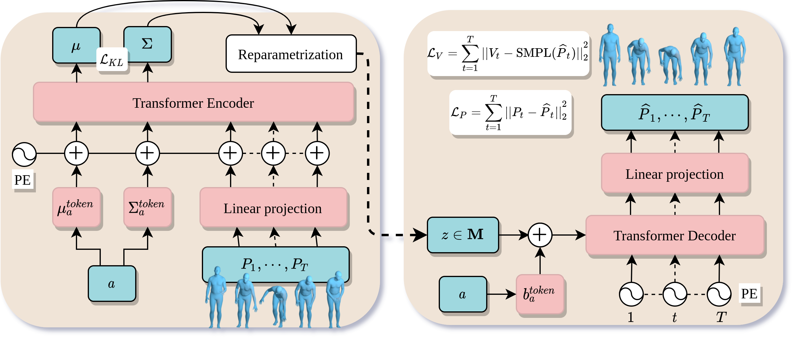
Figure 2: Method overview: We illustrate the encoder (left) and the decoder (right) of our Transformer-based VAE model that generates action-conditioned motions. Given a sequence of body poses $P_{1},\ldots,P_{T}$ and an action label $a$, the encoder outputs distribution parameters on which we define a KL loss ($\mathcal{L}_{KL}$). We use extra learnable tokens per action ($\mu_{a}^{token}$ and $\Sigma_{a}^{token}$) as a way to obtain $\mu$ and $\Sigma$ from the Transformer encoder. Using $\mu$ and $\Sigma$, we sample the motion latent representation $z\in\mathbf{M}$. The decoder takes the latent vector $z$, an action label $a$, and a duration $T$ as input. The action determines the learnable $b_{a}^{token}$ additive token, and the duration determines the number of positional encodings (PE) to input to the decoder. The decoder outputs the whole sequence $\widehat{P}_{1},\ldots,\widehat{P}_{T}$ against which the reconstruction loss $\mathcal{L}_{P}$ is computed. In addition, we compute vertices with a differentiable SMPL layer to define a vertex loss ($\mathcal{L}_{V}$). For training $z$ is obtained as the output of the encoder; for generation it is randomly sampled from a Gaussian distribution.

Many methods for unconstrained motion synthesis are often dominated by actions such as walking and running. In contrast, our model is able to sample from more general, acyclic, pre-defined action categories, compatible with action recognition datasets. In this direction, [75] introduces a Bayesian approach, where Hidden semi-Markov Models are used for jointly training generative and discriminative models. Similar to us, [75] shows that their generated motions can serve as additional training data for action recognition. However, their generated sequences are pseudo-labelled with actions according to the discriminator classification results. On the other hand, our conditional model can synthesize motions in a controlled way, e.g. balanced training set. Most similar to our work is Action2Motion [21], a per-frame VAE on actions, using a GRU-based architecture. Our sequence-level VAE latent space, in conjunction with the Transformer-based design provides significant advantages, as shown in our experiments.

Other recent works [72, 25] use normalizing flows to address human motion estimation and generation problems. Several works [29, 36, 67] learn a motion manifold, and use it for motion denoising, which is one of our use cases.

There is also a significant graphics literature on the topic, which tends to focus on animator control. See, for example, [27] on learning motion matching and [40] on character animation. Most relevant here are the phase-functioned neural networks [28] and neural state machines [61]. Both exploit the notion of actions being driven by the phase of a sinusoidal function. This is related to the idea of positional encoding, but unlike our approach, their methods require manual labor to segment actions and build these phase functions.

Monocular human motion estimation. Motion estimation from videos [35, 38, 47] has recently made significant progress but is beyond our scope. In this work, we adopt VIBE [38] to obtain training motion sequences from action-labelled video datasets.

Transformer VAEs. Recent successes of Transformers in language tasks has increased interest in attention-based neural network models. Several works use Transformers in conjunction with generative VAE training. Particular examples include story generation [15], sentiment analysis [10], response generation [44], and music generation [33]. The work of [33] learns latent embeddings per timeframe, while [10] averages the hidden states to obtain a single latent code. On the other hand, [15] performs attention averaging to pool over time. In contrast to these works, we adopt learnable tokens as in [12, 13] to summarize the input into a sequence-level embedding.

3 Action-Conditioned Motion Generation

Problem definition. Actions defined by body-motions can be characterized by the rotations of body parts, independent of identity-specific body shape. To be able to generate motions with actors of different morphology, it is desirable to disentangle the pose and the shape. Consequently, without loss of generality, we employ the SMPL body model [46], which is a disentangled body representation (similar to recent models [58, 53, 55, 68]). Ignoring shape, our goal, is then to generate a sequence of pose parameters. More formally, given an action label $a$ (from a set of predefined action categories $a\in A$) and a duration $T$, we generate a sequence of body poses $R_{1},\ldots,R_{T}$ and a sequence of translations of the root joint represented as displacements, $D_{1},\ldots,D_{T}$ (with $D_{t}\in\mathbb{R}^{3},\forall t\in\{1,\ldots,T\}$).

Motion representation. SMPL pose parameters per-frame represent 23 joint rotations in the kinematic tree and one global rotation. We adopt the continuous 6D rotation representation for training [76], making $R_{t}\in\mathbb{R}^{24\times 6}$. Let $P_{t}$ be the combination of $R_{t}$ and $D_{t}$, representing the pose and location of the body in a single frame, $t$. The full motion is the sequence $P_{1},\dots,P_{T}$. Given a generator output pose $P_{t}$ and any shape parameter, we can obtain body mesh vertices ($V_{t}$) and body joint coordinates ($J_{t}$) differentiably using [46].

3.1 Conditional Transformer VAE for Motions

We employ a conditional variational autoencoder (CVAE) model [60] and input the action category information to both the encoder and the decoder. More specifically, our model is an action-conditioned Transformer VAE (ACTOR), whose encoder and decoder consist of Transformer layers (see Figure 2 for an overview).

Encoder. The encoder takes an arbitrary-length sequence of poses, and an action label $a$ as input, and outputs distribution parameters $\mu$ and $\Sigma$ of the motion latent space. Using the reparameterization trick [37], we sample from this distribution a latent vector $z\in\mathbf{M}$ with $\mathbf{M}\subset\mathbb{R}^{d}$. All the input pose parameters ($R$) and translations ($D$) are first linearly embedded into a $\mathbb{R}^{d}$ space. As we embed arbitrary-length sequences into one latent space (sequence-level embedding), we need to pool the temporal dimension. In other domains, a [class] token has been introduced for pooling purposes, e.g., in NLP with BERT [12] and more recently in computer vision with ViT [13]. Inspired by this approach, we similarly prepend the inputs with learnable tokens, and only use the corresponding encoder outputs as a way to pool the time dimension. To this end, we include two extra learnable parameters per action, $\mu_{a}^{token}$ and $\Sigma_{a}^{token}$, which we called “distribution parameter tokens”. We append the embedded pose sequences to these tokens. The resulting Transformer encoder input is the summation with the positional encodings in the form of sinusoidal functions. We obtain the distribution parameters $\mu$ and $\Sigma$ by taking the first two outputs of the encoder corresponding to the distribution parameter tokens (i.e., discarding the rest).

Decoder. Given a single latent vector $z$ and an action label $a$, the decoder generates a realistic human motion for a given duration in one shot (i.e., not autoregressive).

We use a Transformer decoder model where we feed time information as a query (in the form of $T$ sinusoidal positional encodings), and the latent vector combined with action information, as key and value. To incorporate the action information, we simply add a learnable bias $b_{a}^{token}$ to shift the latent representation to an action-dependent space. The Transformer decoder outputs a sequence of $T$ vectors in $\mathbb{R}^{d}$ from which we obtain the final poses $\widehat{P}_{1},\ldots,\widehat{P}_{T}$ following a linear projection. A differentiable SMPL layer is used to obtain vertices and joints given the pose parameters as output by the decoder.

3.2 Training

We define several loss terms to train our model and present an ablation study in Section 4.2.

Reconstruction loss on pose parameters ($\mathcal{L}_{P}$). We use an L2 loss between the ground-truth poses $P_{1},\ldots,P_{T}$, and our predictions $\widehat{P}_{1},\ldots,\widehat{P}_{T}$ as $\mathcal{L}_{P}=\sum_{t=1}^{T}\lVert P_{t}-\widehat{P}_{t}\rVert^{2}_{2}$. Note that this loss contains both the SMPL rotations and the root translations. When we experiment by discarding the translations, we break this term into two: $\mathcal{L}_{R}$ and $\mathcal{L}_{D}$, for rotations and translations, respectively.

Reconstruction loss on vertex coordinates ($\mathcal{L}_{V}$). We feed the SMPL poses $P_{t}$ and $\widehat{P}_{t}$ to a differentiable SMPL layer (without learnable parameters) with a mean shape (i.e., $\beta=\vec{0}$) to obtain the root-centered vertices of the mesh $V_{t}$ and $\widehat{V}_{t}$. We define an L2 loss by comparing to the ground-truth vertices ${V}_{t}$ as $\mathcal{L}_{V}=\sum_{t=1}^{T}\lVert V_{t}-\widehat{V}_{t}\rVert^{2}_{2}$ . We further experiment with a loss $\mathcal{L}_{J}$ on a more sparse set of points such as joint locations $\widehat{J}_{t}$ obtained through the SMPL joint regressor. However, as will be shown in Section 4.2, we do not include this term in the final model.

KL loss ($\mathcal{L}_{KL}$). As in a standard VAE, we regularize the latent space by encouraging it to be similar to a Gaussian distribution with $\mu$ the null vector and $\Sigma$ the identity matrix. We minimize the Kullback–Leibler (KL) divergence between the encoder distribution and this target distribution.

The resulting total loss is defined as the summation of different terms: $\mathcal{L}=\mathcal{L}_{P}+\mathcal{L}_{V}+\lambda_{KL}\mathcal{L}_{KL}$. We empirically show the importance of weighting with $\lambda_{KL}$ (equivalent to the $\beta$ term in $\beta$-VAE [26]) in our experiments to obtain a good trade-off between diversity and realism (see Section A.1 of the appendix). The remaining loss terms are simply equally weighed, further improvements are potentially possible with tuning. We use the AdamW optimizer with a fixed learning rate of 0.0001. The minibatch size is set to 20 and we found that the performance is sensitive to this hyperparameter (see Section A.2 of the appendix). We train our model for 2000, 5000 and 1000 epochs on NTU-13, HumanAct12 and UESTC datasets, respectively. Overall, more epochs produce improved performance, but we stop training to retain a low computational cost. Note that to allow faster iterations, for ablations on loss and architecture, we train our models for 1000 epochs on NTU-13 and 500 epochs on UESTC. The remaining implementation details can be found in Section C of the appendix.

4 Experiments

	UESTC					NTU-13
Loss	FIDtr$\downarrow$	FIDtest$\downarrow$	Acc.$\uparrow$	Div.$\rightarrow$	Multimod.$\rightarrow$	FIDtr$\downarrow$	Acc.$\uparrow$	Div.$\rightarrow$	Multimod.$\rightarrow$
Real	$2.93^{\pm 0.26}$	$2.79^{\pm 0.29}$	$98.8^{\pm 0.1}$	$33.34^{\pm 0.32}$	$14.16^{\pm 0.06}$	$0.02^{\pm 0.00}$	$99.8^{\pm 0.0}$	$7.07^{\pm 0.02}$	$2.27^{\pm 0.01}$
$\mathcal{L}_{J}$	$3$M∗	$3$M∗	$3.3^{\pm 0.2}$	$267.68^{\pm 346.06}$	$153.62^{\pm 50.62}$	$0.49^{\pm 0.00}$	$93.6^{\pm 0.2}$	$7.04^{\pm 0.04}$	$2.12^{\pm 0.01}$
$\mathcal{L}_{R}$	$292.54^{\pm 113.35}$	$316.29^{\pm 26.05}$	$42.4^{\pm 1.7}$	$23.16^{\pm 0.47}$	$14.37^{\pm 0.08}$	$0.23^{\pm 0.00}$	$95.4^{\pm 0.2}$	$7.08^{\pm 0\ .04}$	$2.18^{\pm 0.02}$
$\mathcal{L}_{V}$	$4$M∗	$4$M∗	$2.7^{\pm 0.2}$	$314.66^{\pm 476.18}$	$169.49^{\pm 27.90}$	$0.25^{\pm 0.00}$	$95.8^{\ \pm 0.3}$	$7.08^{\pm 0.04}$	$2.07^{\pm 0.01}$
aliceblue $\mathcal{L}_{R}$ + $\mathcal{L}_{V}$	${\bf 20.49}^{\pm 2.31}$	${\bf 23.43}^{\pm 2.20}$	${\bf 91.1}^{\pm 0.3}$	$31.96^{\pm 0.36}$	$14.66^{\pm 0.03}$	${\bf 0.19}^{\pm 0.00}$	${\bf 96.2}^{\pm 0.2}\$	$7.09^{\pm 0.04}$	$2.08^{\pm 0.01}$

Table 1: Reconstruction loss: We define the loss on the SMPL pose parameters which represent the rotations in the kinematic tree ($\mathcal{L}_{R}$), their joint coordinates ($\mathcal{L}_{J}$), as well as vertex coordinates ($\mathcal{L}_{V}$). We show that constraining both rotations and vertex coordinates is critical to obtain smooth motions. In particular, coordinate-based losses alone do not converge to a meaningful solution on UESTC (*). $\rightarrow$ means motions are better when the metric is closer to real.

We first introduce the datasets and performance measures used in our experiments (Section 4.1). Next, we present an ablation study (Section 4.2) and compare to previous work (Section 4.3). Then, we illustrate use cases in action recognition (Sections 4.4). Finally, we provide qualitative results and discuss limitations (Section 4.5).

4.1 Datasets and evaluation metrics

We use three datasets originally proposed for action recognition, mainly for skeleton-based inputs. Each dataset is temporally trimmed around one action per sequence. Next, we briefly describe them.

NTU RGB+D dataset [59, 45]. To be able to compare to the work of [21], we use their subset of 13 action categories. [21] provides SMPL parameters obtained through VIBE estimations. Their 3D root translations, obtained through multi-view constraints, are not publicly available, therefore we use their approximately origin-centered version. We refer to this data as NTU-13 and use it for training.

HumanAct12 dataset [21]. Similarly, we use this data for state-of-the-art comparison. HumanAct12 is adapted from the PHSPD dataset [77] that releases SMPL pose parameters and root translations in camera coordinates for 1191 videos. HumanAct12 temporally trims the videos, annotates them into 12 action categories, and only provides their joint coordinates in a canonical frame. We also process the SMPL poses to align them to the frontal view.

UESTC dataset [32]. This recent dataset consists of 25K sequences across 40 action categories (mostly exercises, and some represent cyclic movements). To obtain SMPL sequences, we apply VIBE on each video and select the person track that corresponds best to the Kinect skeleton provided in case there are multiple people. We use all 8 static viewpoints (we discard the rotating camera) and canonicalize all bodies to the frontal view. We use the official cross-subject protocol to separate train and test splits, instead of the cross-view protocols since generating different viewpoints is trivial for our model. This results in 10650 training sequences that we use for learning the generative model, as well as the recognition model: the effective diversity of this set can be seen as 33 sequences per action on average (10K divided by 8 views, 40 actions). The remaining 13350 sequences are used for testing. Since the protocols on NTU-13 and HumanAct12 do not provide test splits, we rely on UESTC for recognition experiments.

Evaluation metrics. We follow the performance measures employed in [21] for quantitative evaluations. We measure FID, action recognition accuracy, overall diversity, and per-action diversity (referred to as multimodality in [21]). For all these metrics, a pretrained action recognition model is used, either for extracting motion features to compute FID, diversity, and multimodality; or directly the accuracy of recognition. For experiments on NTU-13 and HumanAct12, we directly use the provided recognition models of [21] that operate on joint coordinates. For UESTC, we train our own recognition model based on pose parameters expressed as 6D rotations (we observed that the joint-based models of [21] are sensitive to global viewpoint changes). We generate sets of sequences 20 times with different random seeds and report the average together with the confidence interval at 95%. We refer to [21] for further details. One difference in our evaluation is the use of average shape parameter ($\beta=\vec{0}$) when obtaining joint coordinates from the mesh for both real and generated sequences. Note also that [21] only reports FID score comparing to the training split (FID_tr), since NTU-13 and HumanAct12 datasets do not provide test splits. On UESTC, we additionally provide an FID score on the test split as FID_test, which we rely most on to make conclusions.

	UESTC					NTU-13
Architecture	FIDtr$\downarrow$	FIDtest$\downarrow$	Acc.$\uparrow$	Div.$\rightarrow$	Multimod.$\rightarrow$	FIDtr$\downarrow$	Acc.$\uparrow$	Div.$\rightarrow$	Multimod.$\rightarrow$
Real	$2.93^{\pm 0.26}$	$2.79^{\pm 0.29}$	$98.8^{\pm 0.1}$	$33.34^{\pm 0.32}$	$14.16^{\pm 0.06}$	$0.02^{\pm 0.00}$	$99.8^{\pm 0.0}$	$7.07^{\pm 0.02}$	$2.27^{\pm 0.01}$
Fully connected	$562.09^{\pm 48.12}$	$548.13^{\pm 38.34}$	$10.5^{\pm 0.5}$	$12.96^{\pm 0.11}$	$10.87^{\pm 0.05}$	$0.47^{\pm 0.00}$	$88.7^{\pm 0.6}$	$6.93^{\pm 0.03}$	$3.05^{\pm 0.01}$
GRU	$25.96^{\pm 3.02}$	$27.08^{\pm 2.98}$	$87.3^{\pm 0.4}$	$30.66^{\pm 0.33}$	$15.24^{\pm 0.08}$	$0.28^{\pm 0.00}$	$94.8^{\pm 0.2}$	$7.08^{\pm 0.04}$	$2.20^{\pm 0.01}$
aliceblue Transformer	${\bf 20.49}^{\pm 2.31}$	${\bf 23.43}^{\pm 2.20}$	${\bf 91.1}^{\pm 0.3}$	$31.96^{\pm 0.36}$	$14.66^{\pm 0.03}$	$0.19^{\pm 0.00}$	${\bf 96.2}^{\pm 0.2}$	$7.09^{\pm 0.04}$	$2.08^{\pm 0.01}$
a) w/ autoreg. decoder	$55.75^{\pm 2.62}$	$60.10^{\pm 4.87}$	$88.4^{\pm 0.6}$	$33.46^{\pm 0.69}$	$10.62^{\pm 0.10}$	$2.62^{\pm 0.01}$	$88.0^{\pm 0.5}$	$6.80^{\pm 0.03}$	$1.76^{\pm 0.01}$
b) w/out $\mu_{a}^{token},\Sigma_{a}^{token}$	$27.46^{\pm 3.43}$	$31.37^{\pm 3.04}$	$86.2^{\pm 0.4}$	$31.82^{\pm 0.38}$	$15.71^{\pm 0.12}$	$0.26^{\pm 0.00}$	$94.7^{\pm 0.2}$	$7.09^{\pm 0.03}$	$2.15^{\pm 0.01}$
c) w/out $b_{a}^{token}$	$24.38^{\pm 2.37}$	$28.52^{\pm 2.55}$	$89.4^{\pm 0.7}$	$32.11^{\pm 0.33}$	$14.52^{\pm 0.09}$	${\bf 0.16}^{\pm 0.00}$	${\bf 96.2}^{\pm 0.2}$	$7.08^{\pm 0.04}$	$2.19^{\pm 0.02}$

Table 2: Architecture: We compare various architectural designs, such as the encoder and the decoder of the VAE, and different components of the Transformer model, on both NTU-13 and UESTC datasets.

4.2 Ablation study

We first ablate several components of our approach in a controlled setup, studying the loss and the architecture.

Loss study. Here, we investigate the influence of the reconstruction loss formulation when using the parametric SMPL body model in our VAE. We first experiment with using (i) only the rotation parameters $\mathcal{L}_{R}$, (ii) only the joint coordinates $\mathcal{L}_{J}$, (iii) only the vertex coordinates $\mathcal{L}_{V}$, and (iv) the combination $\mathcal{L}_{R}+\mathcal{L}_{V}$. Here, we initially discard the root translation to only assess the pose representation. Note that for representing the rotation parameters, we use the 6D representation from [76] (further studies on losses with different rotation representations can be found in Section A.4 of the appendix). In Table 1, we observe that a single loss is not sufficient to constrain the problem, especially losses on the coordinates do not converge to a meaningful solution on UESTC. On NTU-13, qualitatively, we also observe invalid body shapes since joint locations alone do not fully constrain the rotations along limb axes. We provide examples in our qualitative analysis. We conclude that using a combined loss significantly improves the results, constraining the pose space more effectively. We further provide an experiment on the influence of the weight parameter $\lambda_{KL}$ controlling the KL divergence loss term $\mathcal{L}_{KL}$ in Section A.1 of the appendix and note its importance to obtain high diversity performance.

Root translation. Since we estimate the 3D human body motion from a monocular camera, obtaining the 3D trajectory of the root joint is not trivial for real training sequences, and is subject to depth ambiguity. We assume a fixed focal length and approximate the distance from the camera based on the ratio between the 3D body height and the 2D projected height. Similar to [65], we observe reliable translation in $xy$ image plane, but considerable noise in $z$ depth. Nevertheless, we still train with this type of data and visualize generated examples in Figure 3 with and without the loss on translation $\mathcal{L}_{D}$. Certain actions are defined by their trajectory (e.g., ‘Left Stretching’) and we are able to generate the semantically relevant translations despite noisy data. Compared to the real sequences, we observe much less noise in our generated sequences (see the supplemental video at [57]).

Architecture design. Next, we ablate several architectural choices. The first question is whether an attention-based design (i.e., Transformer) has advantages over the more widely used alternatives such as a simple fully-connected autoencoder or a GRU-based recurrent neural network. In Table 2, we see that our Transformer model outperforms both fully-connected and GRU encoder-decoder architectures on two datasets by a large margin. In contrast to the fully-connected architecture, we are also able to handle variable-length sequences. We further note that our sequence-level decoding strategy is key to obtain an improvement with Transformers, as opposed to an autoregressive Transformer decoder as in [66] (Table 2, a). At training time, the autoregressive model uses teacher forcing, i.e., using the ground-truth pose for the previous frame. This creates a gap with test time, where we observed poor autoencoding reconstructions such as decoding a left-hand waving encoding into a right-hand waving.

We also provide a controlled experiment by changing certain blocks of our Transformer VAE. Specifically, we remove the $\mu_{a}^{token}$ and $\Sigma_{a}^{token}$ distribution parameter tokens and instead obtain $\mu$ and $\Sigma$ by averaging the outputs of the encoder, followed by two linear layers (Table 2, b). This results in considerable drop in performance. Moreover, we investigate the additive $b_{a}^{token}$ token and replace it with a one-hot encoding of the action label concatenated to the latent vector, followed by a linear projection (Table 2, c). Although this improves a bit the results on the NTU-13 dataset, we observe a large decrease in performance on the UESTC dataset which has a larger number of action classes.

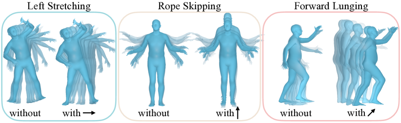
Figure 3: Generating the 3D root translation: Despite our model learning from noisy 3D trajectories, we show that our generations are smooth and they capture the semantics of the action. Examples are provided from the UESTC dataset for translations in $x$ (‘Left Stretching’), $y$ (Rope Skipping), and $z$ (‘Forward Lugging’) with and without the loss on the root displacement $\mathcal{L}_{D}$.

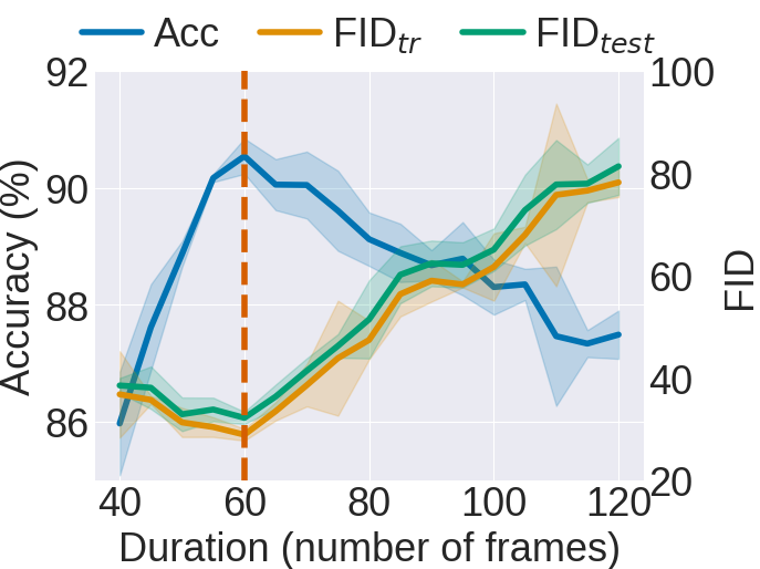
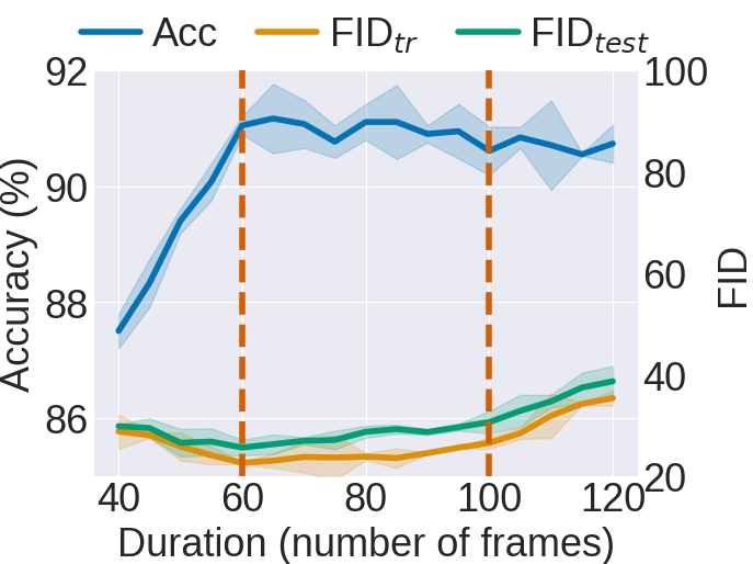
Figure 4: Generating variable-length sequences: We evaluate the capability of the models trained on UESTC with (left) fixed-size 60 frames and (right) variable-size between [60, 100] frames on generating various durations. We report accuracy and FID metrics. For the fixed model, we observe that the best performance is when tested at the seen duration of 60, but over 85% accuracy is retained even at ranges between [40, 120] frames. The performance is overall improved when the model has previously seen duration variations in training; there is a smaller drop in performance beyond the seen range (denoted with dashed lines).

Based on an architectural ablation of the number of Transformer layers (see Section A.3 of the appendix), we set this parameter to 8.

	NTU-13				HumanAct12
Method	FIDtr$\downarrow$	Acc.$\uparrow$	Div.$\rightarrow$	Multimod.$\rightarrow$	FIDtr$\downarrow$	Acc.$\uparrow$	Div.$\rightarrow$	Multimod.$\rightarrow$
Real [21]	$0.03^{\pm 0.00}$	$99.9^{\pm 0.1}$	$7.11^{\pm 0.05}$	$2.19^{\pm 0.03}$	$0.09^{\pm 0.01}$	$99.7^{\pm 0.1}$	$6.85^{\pm 0.05}$	$2.45^{\pm 0.04}$
Real*	$0.02^{\pm 0.00}$	$99.8^{\pm 0.0}$	$7.07^{\pm 0.02}$	$2.25^{\pm 0.01}$	$0.02^{\pm 0.00}$	$99.4^{\pm 0.0}$	$6.86^{\pm 0.03}$	$2.60^{\pm 0.01}$
CondGRU ([21]$\dagger$)	$28.31^{\pm 0.14}$	$7.8^{\pm 0.1}$	$3.66^{\pm 0.02}$	$3.58^{\pm 0.03}$	$40.61^{\pm 0.14}$	$8.0^{\pm 0.2}$	$2.38^{\pm 0.02}$	$2.34^{\pm 0.04}$
Two-stage GAN [9] ([21]$\dagger$)	$13.86^{\pm 0.09}$	$20.2^{\pm 0.3}$	$5.33^{\pm 0.04}$	$3.49^{\pm 0.03}$	$10.48^{\pm 0.09}$	$42.1^{\pm 0.6}$	$5.96^{\pm 0.05}$	$2.81^{\pm 0.04}$
Act-MoCoGAN [62] ([21]$\dagger$)	$2.72^{\pm 0.02}$	${\bf 99.7}^{\pm 0.1}$	$6.92^{\pm 0.06}$	$0.91^{\pm 0.01}$	$5.61^{\pm 0.11}$	$79.3^{\pm 0.4}$	$6.75^{\pm 0.07}$	$1.06^{\pm 0.02}$
Action2Motion [21]	$0.33^{\pm 0.01}$	$94.9^{\pm 0.1}$	$7.07^{\pm 0.04}$	$2.05^{\pm 0.03}$	$2.46^{\pm 0.08}$	$92.3^{\pm 0.2}$	$7.03^{\pm 0.04}$	$2.87^{\pm 0.04}$
aliceblue ACTOR (ours)	${\bf 0.11}^{\pm 0.00}$	$97.1^{\pm 0.2}$	$7.08^{\pm 0.04}$	$2.08^{\pm 0.01}$	${\bf 0.12}^{\pm 0.00}$	${\bf 95.5}^{\pm 0.8}$	$6.84^{\pm 0.03}$	$2.53^{\pm 0.02}$

Table 3: State-of-the-art comparison: We compare to the recent work of [21] on the NTU-13 and HumanAct12 datasets. Note that due to differences in implementation (e.g., random sampling, using zero shape parameter), our metrics for the ground truth real data (Real*) are slightly different than the ones reported in their paper. The performance improvement with our Transformer-based model shows a clear gap from Action2Motion. $\dagger$ Baselines implemented by [21].

Training with sequences of variable durations. A key advantage of sequence-modeling with architectures such as Transformers is to be able to handle variable-length motions. At generation time, we control how long the model should synthesize, by specifying a sequence of positional encodings to the decoder. We can trivially generate more diversity by synthesizing sequences of different durations. However, so far we have trained our models with fixed-size inputs, i.e., 60 frames. Here, we first analyze whether a fixed-size trained model can directly generate variable sizes. This is presented in Figure 4 (left). We plot the performance over several sets of generations of different lengths between 40 and 120 frames (with a step size of 5). Since our recognition model used for evaluation metrics is trained on fixed-size 60-frame inputs, we naturally observe performance decrease outside of this length. However, the accuracy still remains high which indicates that our model is already capable of generating diverse durations.

Next, we train our generative model with variable-length inputs by randomly sampling a sequence between 60 and 100 frames. However, simply training this way from random weight initialization converges to a poor solution, leading all generated motions to be frozen in time. We address this by pretraining at 60-frame fixed size and finetuning at variable sizes. We see in Figure 4 (right) that the performance is greatly improved with this model.

Furthermore, we investigate how the generations longer or shorter than their average durations behave. We observe qualitatively that shorter generations produce partial actions e.g., picking up without reaching the floor, and longer generations slow down somewhat non-uniformly in time. We refer to the supplemental video [57] for qualitative results.

4.3 Comparison to the state of the art

Action2Motion [21] is the only prior work that generates action-conditioned motions. We compare to them in Table 3 on their NTU-13 and HumanAct12 datasets. On both datasets, we obtain significant improvements over this prior work that uses autoregressive GRU blocks, as well as other baselines implemented by [21] by adapting other works [9, 62]. The improvements over [21] can be explained mainly by removing autoregression and adding the proposed learnable tokens (Table 2). Note that our GRU implementation obtains similar performance as [21], while using the same hyperparameters as the Transformer. In addition to the quantitative performance improvement, measured with recognition models based on joint coordinates, our model can directly output human meshes, which can further be diversified with varying the shape parameters. [21] instead applies an optimization step to fit SMPL models on their generated joint coordinates, which is typically substantially slower than a neural network forward pass.

	Test accuracy (%)
	Realorig	Realdenoised
Realorig	91.8	93.2
Realdenoised	83.8	97.0
Realinterpolated	77.6	93.9
Generated	80.7	97.0
Realorig + Generated	91.9	98.3

Table 4: Action recognition: We employ a standard architecture (ST-GCN [70]) and perform action recognition experiments using several sets of training data on the UESTC cross-subject protocol [32]. Training only with generated samples obtains 80% accuracy on the real test set which is another indication our action-conditioning performs well. Nevertheless, we observe a domain gap between generated and real samples, mainly due to the noise present in the real data. We show that simply by encoding-decoding the test sequences, we observe a denoising effect, which in turn shows better performance. However, one should note that the last-column experiments are not meant to improve performance in the benchmark since it uses the action label information.

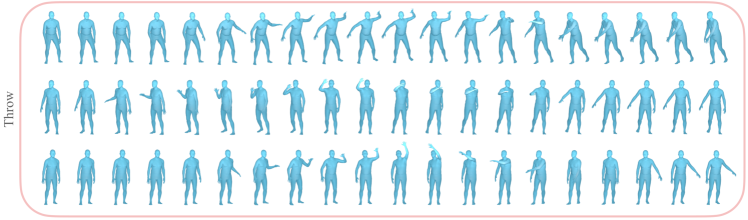
Figure 5: Qualitative results: We illustrate the diversity of our generations on the ‘Throw’ action from NTU-13 by showing 3 sequences. The horizontal axis represent the time axis and 20 equally spaced frames are visualized out of 60-frame generations. We demonstrate that our model is capable of generating different ways of performing a given action. More results can be found in Section B of the appendix and the supplemental video at [57].

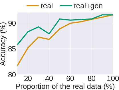
Figure 6: Data augmentation: We show the benefit of augmenting the real data with our generative model (real+gen), especially at low-data regime. We have limited gains when the real data is sufficiently large.

4.4 Use cases in action recognition

In this section, we test the limits of our approach by illustrating the benefits of our generative model and our learned latent representation for the skeleton-based action recognition task. We adopt a standard architecture, ST-GCN [70], that employs spatio-temporal graph convolutions to classify actions. We show that we can use our latent encoding for denoising motion estimates and our generated sequences as data augmentation to action recognition models.

Use case I: Human motion denoising. In the case when our motion data source relies on monocular motion estimation such as [38], the training motions remain noisy. We observe that by simply encoding-decoding the real motions through our learned embedding space, we obtain much cleaner motions. Since it is difficult to show motion quality results on static figures, we refer to our supplemental video at [57] to see this effect. We measure the denoising capability of our model through an action recognition experiment in Table 4. We change both the training and test set motions with the encoded-decoded versions. We show improved performance when trained and tested on Real_denoised motions (97.0%) compared to Real_orig (91.8). Note that this result on its own is not sufficient for this claim, but is only an indication since our decoder might produce less diversity than real motions. Moreover, the action label is given at denoising time. We believe that such denoising can be beneficial in certain scenarios where the action is known, e.g., occlusion or missing markers during MoCap collection.

Use case II: Augmentation for action recognition. Next, we augment the real training data (Real_orig), by adding generated motions to the training. We first measure the action recognition performance without using real sequences. We consider interpolating existing Real_orig motions that fall within the same action category in our embedding space to create intra-class variations (Real_interpolated). We then synthesize motions by sampling noise vectors conditioned on each action category (Generated). Table 4 summarizes the results. Training only on synthetic data performs 80.7% on the real test set, which is promising. However, there is a domain gap between the noisy real motions and our smooth generations. Consequently, adding generated motions to real training only marginally improves the performance. In Figure 6, we investigate whether the augmented training helps for low-data regimes by training at several fractions of the data. In each minibatch we equally sample real and generated motions. However, in theory we have access to infinitely many generations. We see that the improvement is more visible at low-data regime.

4.5 Qualitative results

In Figure 5, we visualize several examples from our generations. We observe a great diversity in the way a given action is performed. For example, the ‘Throw’ action is performed with left or right hand. We notice that the model keeps the essence of the action semantics while changing nuances (angles, speed, phase) or action-irrelevant body parts. We refer to the supplemental video at [57] and Section B of the appendix for further qualitative analyses.

One limitation of our model is that the maximum duration it can generate depends on computational resources since we output all the sequence at once. Moreover, the actions are from a predefined set. Future work will explore open-vocabulary actions, which might become possible with further progress in 3D motion estimation from unconstrained videos.

5 Conclusions

We presented a new Transformer-based VAE model to synthesize action-conditioned human motions. We provided a detailed analysis to assess different components of our proposed approach. We obtained state-of-the-art performance on action-conditioned motion generation, significantly improving over prior work. Furthermore, we explored various use cases in motion denoising and action recognition. One especially attractive property of our method is that it operates on a sequence-level latent space. Future work can therefore exploit our model to impose priors on motion estimation or action recognition problems.

Acknowledgements. This work was granted access to the HPC resources of IDRIS under the allocation 2021-101535 made by GENCI. The authors would like to thank Mathieu Aubry and David Picard for helpful feedback, Chuan Guo and Shihao Zou for their help with Action2Motion details.

Disclosure: MJB has received research funds from Adobe, Intel, Nvidia, Facebook, and Amazon. While MJB is a part-time employee of Amazon, his research was performed solely at, and funded solely by, Max Planck. MJB has financial interests in Amazon, Datagen Technologies, and Meshcapade GmbH.

APPENDIX

We provides additional experiments (Section A), additional qualitative results (Section B), and implementation details (Section C).

Appendix A Additional experiments

We ablate the model and vary key parameters to evaluate the influence of design choices on the quality of the results. In particular, we present results on the effect of $\lambda_{KL}$ (Section A.1), batch size (Section A.2), number of layers (Section A.3), and the rotation representation for SMPL pose parameters (Section A.4).

A.1 Weight of the KL loss

As explained in Section 3.2 of the main paper, we empirically show the importance of the weighting between the reconstruction loss and the KL loss, controlled by $\lambda_{KL}$. Table A.1 presents results for several values of $\lambda_{KL}$ and we find that there is a trade-off between diversity and realism that is best balanced at $\lambda_{KL}=1\mathrm{e}{-5}$. We use this value in all our experiments.

A.2 Influence of the batch size

As pointed out in Section 3.2 of the main paper, we find that the batch size significantly influences the performance. In Table A.2, we report results with batch sizes of 10, 20, 30, 40 for a fixed learning rate. The best performance is obtained at 20, which is used in all our experiments.

A.3 Number of layers

We experiment with the number of Transformer layers in both of our encoder and decoder architectures. Table A.3 summarizes the results. While 2 and 4 layers are sub-optimal, the performance difference between 6 and 8 layers is minimal. We use 8 layers in all our experiments.

A.4 SMPL pose parameter representation

In Table A.4, we explore different rotation representations for SMPL pose parameters. Note that we also preserve the loss on the vertices $\mathcal{L}_{V}$ in all rows. We find that an axis-angle representation is difficult to train due to discontinuities, while others, such as quaternions, rotation matrices and 6D continuous representations [76] are similar in performance on NTU-13. On UESTC, we obtain the best performance with the 6D representation and use this in all our experiments.

Appendix B Additional qualitative results

Figure A.1 demonstrates the diversity of our generated motions for additional actions on NTU-13 and UESTC.

Video. We provide a supplemental video at [57] to illustrate qualitatively the diversity in our generations and compare with Action2Motion [21]. Moreover, we visualize the effect of using a combined reconstruction loss defined both on rotations and vertex coordinates, as opposed to a single loss. We further present results of changing the duration of the generations. We also inspect the latent space by interpolating the noise vector. Finally, we present the denoising capability of our model by encoding-decoding through our latent space. This takes jerky motions and produces smooth but natural looking motion.

Jitter removal for Action2Motion [21]. Besides the quantitative improvement of ACTOR over Action2Motion, we observe qualitatively that Action2Motion generations have significant temporal jitter. To investigate whether our improvement stems from this difference, we removed jitter (using 1€ filter) from Action2Motion generations (that we obtained with their code). The result becomes worse (FID: 0.41 $\rightarrow$ 0.63, Acc: 94.3% $\rightarrow$ 93.0%), perhaps because the real data also has considerable jitter. This suggests that our significant quantitative improvement can be attributed to other factors such as more distinguishable actions.

Appendix C Implementation details

Architectural details. For all our experiments, we set the embedding dimensionality to 256. In the Transformer, we set the number of layers to 8, the number of heads in multi-head attention to 4, the dropout rate to 0.1 and the dimension of the intermediate feedforward network to 1024. As in GPT-3 [8] and BERT [12], we use Gaussian Linear Error Units (GELU) [24] in our Transformer architecture.

Library credits. Our models are implemented with PyTorch [54], and we use PyTorch3D [34] to perform differentiable conversion between rotation representations. We integrate the differentiable SMPL layer using the PyTorch implementation of SMPL-X [55].

Metrics. For the evaluation metrics, we use the implementations provided by Action2Motion [21].

Runtime. Training takes 24 hours for 2K epochs on NTU, 19h hours for 5K epochs on HumanAct12, and 33 hours for 1K epochs on UESTC on a single Tesla V100 GPU, using 4GB GPU memory with batch size 20.

Training with sequences of variable durations. As explained in Section 4.2 of the main paper, we finetune our model with variable-durations after pretraining on fixed-durations. For this, we restore the model weights from the fixed-duration pretraining and finetune for 100 additional epochs, with the same training hyperparameters.

	UESTC					NTU-13
	FIDtr$\downarrow$	FIDtest$\downarrow$	Acc.$\uparrow$	Div.$\rightarrow$	Multimod.$\rightarrow$	FIDtr$\downarrow$	Acc.$\uparrow$	Div.$\rightarrow$	Multimod.$\rightarrow$
Real	$2.93^{\pm 0.26}$	$2.79^{\pm 0.29}$	$98.8^{\pm 0.1}$	$33.34^{\pm 0.32}$	$14.16^{\pm 0.06}$	$0.02^{\pm 0.00}$	$99.8^{\pm 0.0}$	$7.07^{\pm 0.02}$	$2.27^{\pm 0.01}$
$\lambda_{KL}=1\mathrm{e}{-3}$	$460.72^{\pm 90.36}$	$490.12^{\pm 36.10}$	$34.4^{\pm 1.4}$	$20.69^{\pm 0.60}$	$1.25^{\pm 0.00}$	$13.79^{\pm 0.03}$	$46.6^{\pm 0.7}$	$5.79^{\pm 0.04}$	$1.53^{\pm 0.01}$
$\lambda_{KL}=1\mathrm{e}{-4}$	$367.95^{\pm 94.07}$	$390.68^{\pm 41.02}$	$38.1^{\pm 0.9}$	$20.91^{\pm 0.38}$	$9.19^{\pm 0.08}$	$9.90^{\pm 0.02}$	$50.3^{\pm 1.0}$	$6.15^{\pm 0.04}$	$2.86^{\pm 0.02}$
aliceblue $\lambda_{KL}=1\mathrm{e}{-5}$	$20.02^{\pm 1.79}$	$23.64^{\pm 3.59}$	$90.5^{\pm 0.4}$	$32.77^{\pm 0.48}$	$14.64^{\pm 0.07}$	$0.17^{\pm 0.00}$	$96.4^{\pm 0.2}$	$7.08^{\pm 0.03}$	$2.12^{\pm 0.01}$
$\lambda_{KL}=1\mathrm{e}{-6}$	$34.13^{\pm 5.52}$	$39.74^{\pm 3.57}$	$77.4^{\pm 0.8}$	$29.60^{\pm 0.35}$	$18.08^{\pm 0.08}$	$13.83^{\pm 0.03}$	$46.6^{\pm 0.7}$	$5.78^{\pm 0.04}$	$1.54^{\pm 0.01}$
$\lambda_{KL}=1\mathrm{e}{-7}$	$80.05^{\pm 7.71}$	$83.68^{\pm 12.55}$	$47.1^{\pm 2.1}$	$25.06^{\pm 0.15}$	$19.96^{\pm 0.08}$	$7.04^{\pm 0.03}$	$43.0^{\pm 2.1}$	$6.17^{\pm 0.03}$	$4.18^{\pm 0.01}$

Table A.1: Weighting the KL loss term: To obtain a good trade-off between diversity and realism, it is important to find the balance between the reconstruction loss term and the KL loss term in training. We set the weight $\lambda_{KL}$ to $1\mathrm{e}{-5}$ in our training.

	UESTC					NTU-13
	FIDtr$\downarrow$	FIDtest$\downarrow$	Acc.$\uparrow$	Div.$\rightarrow$	Multimod.$\rightarrow$	FIDtr$\downarrow$	Acc.$\uparrow$	Div.$\rightarrow$	Multimod.$\rightarrow$
Real	$2.93^{\pm 0.26}$	$2.79^{\pm 0.29}$	$98.8^{\pm 0.1}$	$33.34^{\pm 0.32}$	$14.16^{\pm 0.06}$	$0.02^{\pm 0.00}$	$99.8^{\pm 0.0}$	$7.07^{\pm 0.02}$	$2.27^{\pm 0.01}$
Batch size = 10	$283.28^{\pm 94.40}$	$309.15^{\pm 33.90}$	$39.7^{\pm 1.5}$	$23.24^{\pm 0.43}$	$15.73^{\pm 0.11}$	$13.95^{\pm 0.03}$	$46.2^{\pm 0.6}$	$5.77^{\pm 0.05}$	$1.56^{\pm 0.01}$
aliceblue Batch size = 20	$20.02^{\pm 1.79}$	$23.64^{\pm 3.59}$	$90.5^{\pm 0.4}$	$32.77^{\pm 0.48}$	$14.64^{\pm 0.07}$	$0.17^{\pm 0.00}$	$96.4^{\pm 0.2}$	$7.08^{\pm 0.03}$	$2.12^{\pm 0.01}$
Batch size = 30	$23.37^{\pm 2.95}$	$26.06^{\pm 1.28}$	$89.7^{\pm 0.5}$	$32.07^{\pm 0.58}$	$14.59^{\pm 0.05}$	$0.18^{\pm 0.00}$	$96.2^{\pm 0.2}$	$7.07^{\pm 0.04}$	$2.13^{\pm 0.01}$
Batch size = 40	$25.36^{\pm 1.82}$	$28.22^{\pm 2.16}$	$89.2^{\pm 0.7}$	$32.22^{\pm 0.44}$	$14.52^{\pm 0.10}$	$0.26^{\pm 0.00}$	$95.4^{\pm 0.1}$	$7.06^{\pm 0.05}$	$2.10^{\pm 0.01}$

Table A.2: Batch size: We observe sensitivity of the Transformer VAE training to different batch sizes and report performances at several batch size values. We set this hyperparameter to 20 in our training.

	UESTC					NTU-13
	FIDtr$\downarrow$	FIDtest$\downarrow$	Acc.$\uparrow$	Div.$\rightarrow$	Multimod.$\rightarrow$	FIDtr$\downarrow$	Acc.$\uparrow$	Div.$\rightarrow$	Multimod.$\rightarrow$
Real	$2.93^{\pm 0.26}$	$2.79^{\pm 0.29}$	$98.8^{\pm 0.1}$	$33.34^{\pm 0.32}$	$14.16^{\pm 0.06}$	$0.02^{\pm 0.00}$	$99.8^{\pm 0.0}$	$7.07^{\pm 0.02}$	$2.27^{\pm 0.01}$
2-layers	$34.66^{\pm 2.58}$	$37.17^{\pm 3.53}$	$84.9^{\pm 0.6}$	$30.87^{\pm 0.36}$	$15.83^{\pm 0.08}$	$0.24^{\pm 0.00}$	$94.6^{\pm 0.2}$	$7.07^{\pm 0.03}$	$2.22^{\pm 0.01}$
4-layers	$23.93^{\pm 1.50}$	$26.75^{\pm 1.99}$	$88.9^{\pm 0.5}$	$32.24^{\pm 0.76}$	$15.06^{\pm 0.06}$	$0.19^{\pm 0.00}$	$96.1^{\pm 0.2}$	$7.09^{\pm 0.04}$	$2.10^{\pm 0.01}$
6-layers	$21.68^{\pm 1.78}$	$24.92^{\pm 2.09}$	$89.0^{\pm 0.6}$	$32.61^{\pm 0.41}$	$15.31^{\pm 0.05}$	$0.16^{\pm 0.00}$	$96.6^{\pm 0.1}$	$7.09^{\pm 0.04}$	$2.11^{\pm 0.01}$
aliceblue 8-layers	$20.02^{\pm 1.79}$	$23.64^{\pm 3.59}$	$90.5^{\pm 0.4}$	$32.77^{\pm 0.48}$	$14.64^{\pm 0.07}$	$0.17^{\pm 0.00}$	$96.4^{\pm 0.2}$	$7.08^{\pm 0.03}$	$2.12^{\pm 0.01}$

Table A.3: Number of layers: We use 8 layers in both the encoder and the decoder of the Transformer VAE. While the performance degrades at 2 or 4 layers, we see marginal gains after 6 layers.

	UESTC					NTU-13
	FIDtr$\downarrow$	FIDtest$\downarrow$	Acc.$\uparrow$	Div.$\rightarrow$	Multimod.$\rightarrow$	FIDtr$\downarrow$	Acc.$\uparrow$	Div.$\rightarrow$	Multimod.$\rightarrow$
Real	$2.93^{\pm 0.26}$	$2.79^{\pm 0.29}$	$98.8^{\pm 0.1}$	$33.34^{\pm 0.32}$	$14.16^{\pm 0.06}$	$0.02^{\pm 0.00}$	$99.8^{\pm 0.0}$	$7.07^{\pm 0.02}$	$2.27^{\pm 0.01}$
Axis-angle	$513.39^{\pm 98.35}$	$531.88^{\pm 43.41}$	$16.4^{\pm 0.4}$	$19.75^{\pm 0.44}$	$1.81^{\pm 0.00}$	$14.98^{\pm 0.03}$	$41.7^{\pm 0.7}$	$5.29^{\pm 0.02}$	$1.96^{\pm 0.01}$
Quaternion	$281.9^{\pm 87.5}$	$305.02^{\pm 21.97}$	$41.2^{\pm 1.0}$	$23.48^{\pm 0.39}$	$14.57^{\pm 0.06}$	$0.20^{\pm 0.00}$	$95.6^{\pm 0.3}$	$7.08^{\pm 0.04}$	$2.23^{\pm 0.01}$
Rotation matrix	$277.14^{\pm 76.59}$	$300.29^{\pm 29.53}$	$41.6^{\pm 1.9}$	$22.25^{\pm 0.30}$	$14.56^{\pm 0.10}$	$0.17^{\pm 0.00}$	$95.9^{\pm 0.2}$	$7.08^{\pm 0.04}$	$2.19^{\pm 0.01}$
aliceblue 6D continuous	$20.02^{\pm 1.79}$	$23.64^{\pm 3.59}$	$90.5^{\pm 0.4}$	$32.77^{\pm 0.48}$	$14.64^{\pm 0.07}$	$0.17^{\pm 0.00}$	$96.4^{\pm 0.2}$	$7.08^{\pm 0.03}$	$2.12^{\pm 0.01}$

Table A.4: SMPL pose parameter representation: We investigate different rotation representations for the SMPL pose parameters. While on NTU-13, all except axis-angle representations perform similarly, the best performing representation on UESTC is the 6D continuous representation [76]. Note that the action recognition model which is used for evaluation is based on 6D rotations on UESTC and joint coordinates on NTU-13. Therefore, we convert each generation to these representations before evaluation.

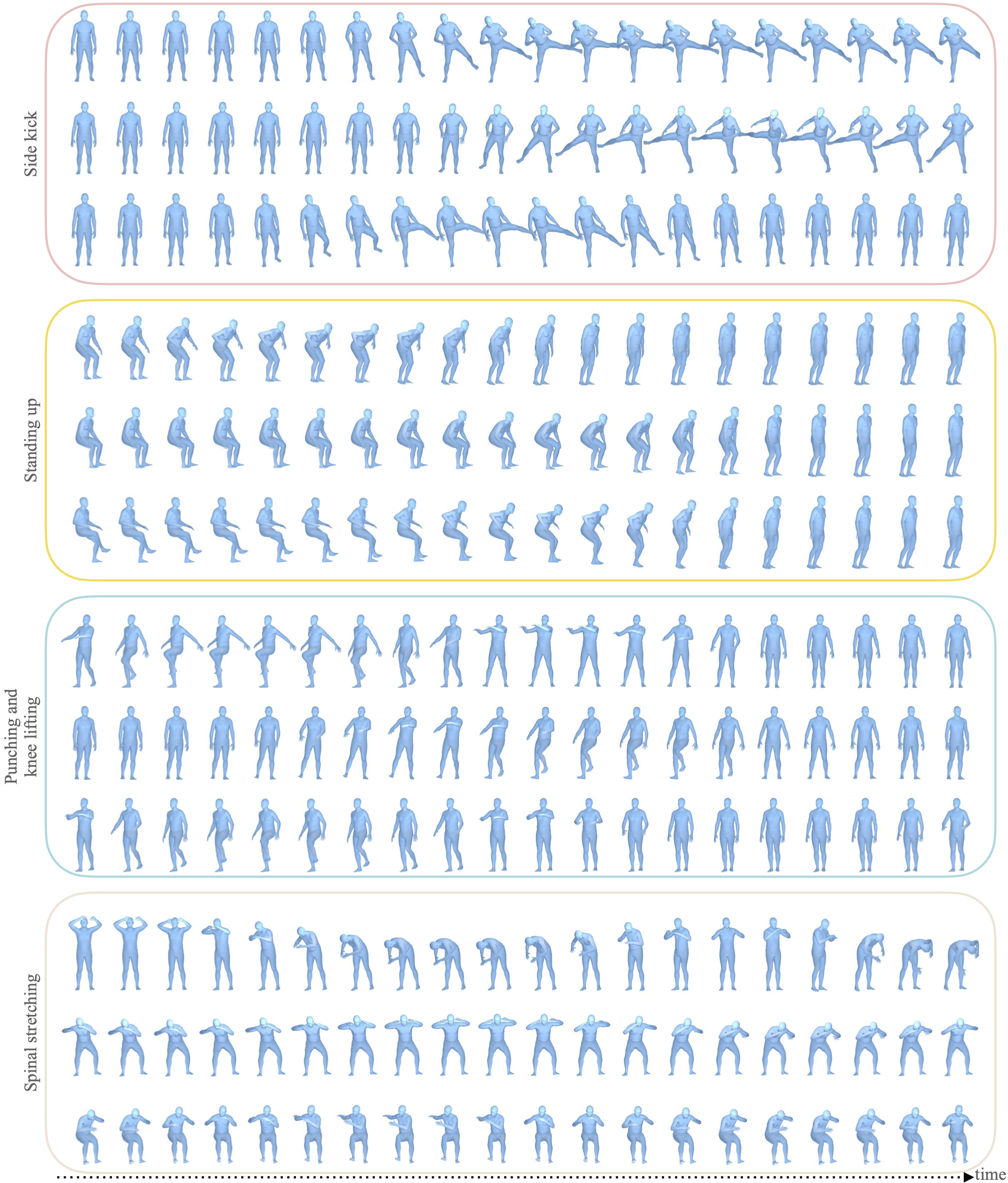
Figure A.1: Additional qualitative results: We provide more action categories from NTU-13 (top two actions: ‘Side kick’ and ‘Standing up’) and UESTC (bottom two actions: ‘Punching and knee lifting’ and ‘Spinal stretching’). As in Section 5 of the main paper, we show 3 generations per action. Our model generates different ways to perform the same action.

References

- [1] Hyemin Ahn, Timothy Ha, Yunho Choi, Hwiyeon Yoo, and Songhwai Oh. Text2Action: Generative adversarial synthesis from language to action. In International Conference on Robotics and Automation (ICRA), pages 5915–5920, 2018.
- [2] Chaitanya Ahuja and Louis-Philippe Morency. Language2Pose: Natural language grounded pose forecasting. In 2019 International Conference on 3D Vision (3DV), pages 719–728, 2019.
- [3] Emre Aksan, Manuel Kaufmann, and Otmar Hilliges. Structured prediction helps 3D human motion modelling. In International Conference on Computer Vision (ICCV), pages 7143–7152, 2019.
- [4] Norman Badler. Temporal Scene Analysis: Conceptual Descriptions of Object Movements. PhD thesis, University of Toronto, 1975.
- [5] Norman I. Badler, Cary B. Phillips, and Bonnie Lynn Webber. Simulating Humans: Computer Graphics Animation and Control. Oxford University Press, Inc., New York, NY, USA, 1993.
- [6] Emad Barsoum, John Kender, and Zicheng Liu. HP-GAN: Probabilistic 3D human motion prediction via GAN. In Conference on Computer Vision and Pattern Recognition Workshops (CVPRW), pages 1499–149909, 2018.
- [7] Richard Bowden. Learning statistical models of human motion. In Conference on Computer Vision and Pattern Recognition (CVPR), Workshop on Human Modeling, Analysis and Synthesis, 2000.
- [8] Tom B. Brown, Benjamin Mann, Nick Ryder, Melanie Subbiah, Jared Kaplan, Prafulla Dhariwal, Arvind Neelakantan, Pranav Shyam, Girish Sastry, Amanda Askell, Sandhini Agarwal, Ariel Herbert-Voss, Gretchen Krueger, Tom Henighan, Rewon Child, Aditya Ramesh, Daniel M. Ziegler, Jeffrey Wu, Clemens Winter, Christopher Hesse, Mark Chen, Eric Sigler, Mateusz Litwin, Scott Gray, Benjamin Chess, Jack Clark, Christopher Berner, Sam McCandlish, Alec Radford, Ilya Sutskever, and Dario Amodei. Language models are few-shot learners. In Advances in Neural Information Processing Systems (NeurIPS), 2020.
- [9] Haoye Cai, Chunyan Bai, Yu-Wing Tai, and Chi-Keung Tang. Deep video generation, prediction and completion of human action sequences. In European Conference on Computer Vision (ECCV), pages 374–390, 2018.
- [10] Xingyi Cheng, Weidi Xu, Taifeng Wang, Wei Chu, Weipeng Huang, Kunlong Chen, and Junfeng Hu. Variational semi-supervised aspect-term sentiment analysis via transformer. In Computational Natural Language Learning (CoNLL), pages 961–969, 2019.
- [11] Enric Corona, Albert Pumarola, Guillem Alenyà, and Francesc Moreno-Noguer. Context-aware human motion prediction. In Conference on Computer Vision and Pattern Recognition (CVPR), pages 6990–6999, 2020.
- [12] Jacob Devlin, Ming-Wei Chang, Kenton Lee, and Kristina Toutanova. BERT: Pre-training of deep bidirectional transformers for language understanding. In North American Chapter of the Association for Computational Linguistics (NAACL), pages 4171–4186, 2019.
- [13] Alexey Dosovitskiy, Lucas Beyer, Alexander Kolesnikov, Dirk Weissenborn, Xiaohua Zhai, Thomas Unterthiner, Mostafa Dehghani, Matthias Minderer, Georg Heigold, Sylvain Gelly, et al. An image is worth 16x16 words: Transformers for image recognition at scale. In International Conference on Learning Representations (ICLR), 2021.
- [14] Yinglin Duan, Tianyang Shi, Zhengxia Zou, Yenan Lin, Zhehui Qian, Bohan Zhang, and Yi Yuan. Single-shot motion completion with transformer. arXiv:2103.00776, 2021.
- [15] Le Fang, Tao Zeng, Chaochun Liu, Liefeng Bo, Wen Dong, and Changyou Chen. Transformer-based conditional variational autoencoder for controllable story generation. arXiv:2101.00828, 2021.
- [16] Katerina Fragkiadaki, Sergey Levine, Panna Felsen, and Jitendra Malik. Recurrent network models for human dynamics. In International Conference on Computer Vision (ICCV), pages 4346–4354, 2015.
- [17] Robert P. Futrelle and Glen C. Speckert. Extraction of motion data by interactive processing. In Conference Pattern Recognition and Image Processing (CP), pages 405–408, 1978.
- [18] Aphrodite Galata, Neil Johnson, and David Hogg. Learning variable length markov models of behaviour. Computer Vision and Image Understanding (CVIU), 81:398–413, 2001.
- [19] Dariu M. Gavrila. The visual analysis of human movement: A survey. Computer Vision and Image Understanding (CVIU), 73:82–98, 1999.
- [20] Ian Goodfellow, Jean Pouget-Abadie, Mehdi Mirza, Bing Xu, David Warde-Farley, Sherjil Ozair, Aaron Courville, and Yoshua Bengio. Generative adversarial nets. In Advances in Neural Information Processing Systems (NeurIPS), volume 27, 2014.
- [21] Chuan Guo, Xinxin Zuo, Sen Wang, Shihao Zou, Qingyao Sun, Annan Deng, Minglun Gong, and Li Cheng. Action2motion: Conditioned generation of 3d human motions. In ACM International Conference on Multimedia (ACMMM), pages 2021–2029, 2020.
- [22] Ikhsanul Habibie, Daniel Holden, Jonathan Schwarz, Joe Yearsley, and Taku Komura. A recurrent variational autoencoder for human motion synthesis. In British Machine Vision Conference (BMVC), pages 119.1–119.12, 2017.
- [23] Félix G. Harvey, Mike Yurick, Derek Nowrouzezahrai, and C. Pal. Robust motion in-betweening. ACM Transactions on Graphics (TOG), 39:60:1 – 60:12, 2020.
- [24] Dan Hendrycks and Kevin Gimpel. Gaussian error linear units (GELUs). arXiv:1606.08415, 2016.
- [25] Gustav Eje Henter, Simon Alexanderson, and Jonas Beskow. MoGlow: Probabilistic and controllable motion synthesis using normalising flows. ACM Transactions on Graphics (TOG), 39(6), 2020.
- [26] Irina Higgins, Loic Matthey, Arka Pal, Christopher Burgess, Xavier Glorot, Matt Botvinick, Shakir Mohamed, and Alexander Lerchner. beta-VAE: Learning basic visual concepts with a constrained variational framework. In International Conference on Learning Representations (ICLR), 2017.
- [27] Daniel Holden, Oussama Kanoun, Maksym Perepichka, and Tiberiu Popa. Learned motion matching. ACM Transactions on Graphics (TOG), 39:53:1 – 53:12, 2020.
- [28] Daniel Holden, Taku Komura, and Jun Saito. Phase-functioned neural networks for character control. ACM Transactions on Graphics (TOG), 36(4), 2017.
- [29] Daniel Holden, Jun Saito, and Taku Komura. A deep learning framework for character motion synthesis and editing. ACM Transactions on Graphics (TOG), 35(4), 2016.
- [30] Catalin Ionescu, Fuxin Li, and Cristian Sminchisescu. Latent structured models for human pose estimation. In International Conference on Computer Vision (ICCV), pages 2220–2227, 2011.
- [31] Catalin Ionescu, Dragos Papava, Vlad Olaru, and Cristian Sminchisescu. Human3.6M: Large scale datasets and predictive methods for 3D human sensing in natural environments. IEEE Transactions on Pattern Analysis and Machine Intelligence (TPAMI), 36(7):1325–1339, 2014.
- [32] Yanli Ji, Feixiang Xu, Yang Yang, Fumin Shen, Heng Tao Shen, and Wei-Shi Zheng. A large-scale RGB-D database for arbitrary-view human action recognition. In ACM International Conference on Multimedia (ACMMM), page 1510–1518, 2018.
- [33] Junyan Jiang, Gus G. Xia, Dave B. Carlton, Chris N. Anderson, and Ryan H. Miyakawa. Transformer VAE: A hierarchical model for structure-aware and interpretable music representation learning. In IEEE International Conference on Acoustics, Speech and Signal Processing (ICASSP), pages 516–520, 2020.
- [34] Justin Johnson, Nikhila Ravi, Jeremy Reizenstein, David Novotny, Shubham Tulsiani, Christoph Lassner, and Steve Branson. Accelerating 3D deep learning with PyTorch3D. In SIGGRAPH Asia 2020 Courses, 2020.
- [35] Angjoo Kanazawa, Jason Y. Zhang, Panna Felsen, and Jitendra Malik. Learning 3D human dynamics from video. In Conference on Computer Vision and Pattern Recognition (CVPR), pages 5607–5616, 2019.
- [36] Seong Uk Kim, Hanyoung Jang, and Jongmin Kim. Human motion denoising using attention-based bidirectional recurrent neural network. In SIGGRAPH Asia, 2019.
- [37] Diederik P Kingma and Max Welling. Auto-encoding variational bayes. In International Conference on Learning Representations (ICLR), 2014.
- [38] Muhammed Kocabas, Nikos Athanasiou, and Michael J. Black. Vibe: Video inference for human body pose and shape estimation. In Conference on Computer Vision and Pattern Recognition (CVPR), pages 5252–5262, 2020.
- [39] Hsin-Ying Lee, Xiaodong Yang, Ming-Yu Liu, Ting-Chun Wang, Yu-Ding Lu, Ming-Hsuan Yang, and Jan Kautz. Dancing to music. In Advances in Neural Information Processing Systems (NeurIPS), 2019.
- [40] Kyungho Lee, Seyoung Lee, and Jehee Lee. Interactive character animation by learning multi-objective control. ACM Transactions on Graphics (TOG), 2018.
- [41] Jiaman Li, Yihang Yin, Hang Chu, Yi Zhou, Tingwu Wang, Sanja Fidler, and Hao Li. Learning to generate diverse dance motions with transformer. arXiv:2008.08171, 2020.
- [42] Ruilong Li, Shan Yang, David A. Ross, and Angjoo Kanazawa. Ai choreographer: Music conditioned 3D dance generation with AIST++, 2021.
- [43] X. Lin and M. Amer. Human motion modeling using DVGANs. arXiv:1804.10652, 2018.
- [44] Zhaojiang Lin, Genta Indra Winata, Peng Xu, Zihan Liu, and Pascale Fung. Variational transformers for diverse response generation. arXiv:2003.12738, 2020.
- [45] Jun Liu, Amir Shahroudy, Mauricio Perez, Gang Wang, Ling-Yu Duan, and Alex C. Kot. NTU RGB+D 120: A large-scale benchmark for 3D human activity understanding. IEEE Transactions on Pattern Analysis and Machine Intelligence (TPAMI), pages 1–18, 2019.
- [46] Matthew Loper, Naureen Mahmood, Javier Romero, Gerard Pons-Moll, and Michael J. Black. SMPL: A skinned multi-person linear model. ACM Transactions on Graphics (TOG), 34(6), Oct. 2015.
- [47] Zhengyi Luo, S. Alireza Golestaneh, and Kris M. Kitani. 3D human motion estimation via motion compression and refinement. In Asian Conference on Computer Vision (ACCV), 2020.
- [48] Naureen Mahmood, Nima Ghorbani, Nikolaus F. Troje, Gerard Pons-Moll, and Michael Black. AMASS: Archive of motion capture as surface shapes. In International Conference on Computer Vision (ICCV), pages 5441–5450, 2019.
- [49] Julieta Martinez, Michael J. Black, and Javier Romero. On human motion prediction using recurrent neural networks. In Conference on Computer Vision and Pattern Recognition (CVPR), pages 4674–4683, 2017.
- [50] Ben Mildenhall, Pratul P. Srinivasan, Matthew Tancik, Jonathan T. Barron, Ravi Ramamoorthi, and Ren Ng. NeRF: Representing scenes as neural radiance fields for view synthesis. In European Conference on Computer Vision (ECCV), pages 405–421, 2020.
- [51] Dirk Ormoneit, Michael J. Black, Trevor Hastie, and Hedvig Kjellström. Representing cyclic human motion using functional analysis. Image and Vision Computing, 23(14):1264–1276, 2005.
- [52] Joseph O’Rourke and Norman I. Badler. Model-based image analysis of human motion using constraint propagation. IEEE Transactions on Pattern Analysis and Machine Intelligence (TPAMI), PAMI-2(6):522–536, 1980.
- [53] Ahmed A. A. Osman, Timo Bolkart, and Michael J. Black. STAR: Sparse trained articulated human body regressor. In European Conference on Computer Vision (ECCV), pages 598–613, 2020.
- [54] Adam Paszke, Sam Gross, Francisco Massa, Adam Lerer, James Bradbury, Gregory Chanan, Trevor Killeen, Zeming Lin, Natalia Gimelshein, Luca Antiga, Alban Desmaison, Andreas Kopf, Edward Yang, Zachary DeVito, Martin Raison, Alykhan Tejani, Sasank Chilamkurthy, Benoit Steiner, Lu Fang, Junjie Bai, and Soumith Chintala. PyTorch: An imperative style, high-performance deep learning library. In Advances in Neural Information Processing Systems (NeurIPS), 2019.
- [55] Georgios Pavlakos, Vasileios Choutas, Nima Ghorbani, Timo Bolkart, Ahmed A. Osman, Dimitrios Tzionas, and Michael J. Black. Expressive body capture: 3D hands, face, and body from a single image. In Conference on Computer Vision and Pattern Recognition (CVPR), pages 10967–10977, 2019.
- [56] Dario Pavllo, David Grangier, and Michael Auli. QuaterNet: A quaternion-based recurrent model for human motion. In British Machine Vision Conference (BMVC), 2018.
- [57] Mathis Petrovich, Michael J. Black, and Gül Varol. ACTOR project page: Action-conditioned 3D human motion synthesis with Transformer VAE. https://imagine.enpc.fr/~petrovim/actor.
- [58] Javier Romero, Dimitrios Tzionas, and Michael J. Black. Embodied hands: Modeling and capturing hands and bodies together. ACM Transactions on Graphics (TOG), 36(6), 2017.
- [59] Amir Shahroudy, Jun Liu, Tian-Tsong Ng, and Gang Wang. NTU RGB+D: A large scale dataset for 3d human activity analysis. In Conference on Computer Vision and Pattern Recognition (CVPR), pages 1010–1019, 2016.
- [60] Kihyuk Sohn, Honglak Lee, and Xinchen Yan. Learning structured output representation using deep conditional generative models. In Advances in Neural Information Processing Systems (NeurIPS), volume 28. Curran Associates, Inc., 2015.
- [61] Sebastian Starke, He Zhang, Taku Komura, and Jun Saito. Neural state machine for character-scene interactions. ACM Transactions on Graphics (TOG), 38(6), 2019.
- [62] Sergey Tulyakov, Ming-Yu Liu, Xiaodong Yang, and Jan Kautz. MoCoGAN: Decomposing motion and content for video generation. In Conference on Computer Vision and Pattern Recognition (CVPR), pages 1526–1535, 2018.
- [63] Carnegie Mellon University. CMU graphics lab motion capture database. http://mocap.cs.cmu.edu/.
- [64] Raquel Urtasun, David J. Fleet, and Neil D. Lawrence. Modeling human locomotion with topologically constrained latent variable models. In Ahmed Elgammal, Bodo Rosenhahn, and Reinhard Klette, editors, Human Motion – Understanding, Modeling, Capture and Animation, pages 104–118, 2007.
- [65] Gül Varol, Ivan Laptev, Cordelia Schmid, and Andrew Zisserman. Synthetic humans for action recognition from unseen viewpoints. International Journal of Computer Vision (IJCV), page 2264–2287, 2021.
- [66] Ashish Vaswani, Noam Shazeer, Niki Parmar, Jakob Uszkoreit, Llion Jones, Aidan N Gomez, Lukasz Kaiser, and Illia Polosukhin. Attention is all you need. In Advances in Neural Information Processing Systems (NeurIPS), volume 30, 2017.
- [67] He Wang, Edmond S. L. Ho, Hubert P. H. Shum, and Zhanxing Zhu. Spatio-temporal manifold learning for human motions via long-horizon modeling. IEEE Transactions on Visualization and Computer Graphics (TVCG), 27:216–227, 2021.
- [68] Hongyi Xu, Eduard Gabriel Bazavan, Andrei Zanfir, William T. Freeman, Rahul Sukthankar, and Cristian Sminchisescu. GHUM and GHUML: Generative 3D human shape and articulated pose models. In Conference on Computer Vision and Pattern Recognition (CVPR), pages 6183–6192, 2020.
- [69] Sijie Yan, Zhizhong Li, Yuanjun Xiong, Huahan Yan, and Dahua Lin. Convolutional sequence generation for skeleton-based action synthesis. In International Conference on Computer Vision (ICCV), pages 4393–4401, 2019.
- [70] Sijie Yan, Yuanjun Xiong, and Dahua Lin. Spatial temporal graph convolutional networks for skeleton-based action recognition. In AAAI Conference on Artificial Intelligence, 2018.
- [71] Ye Yuan and Kris Kitani. Dlow: Diversifying latent flows for diverse human motion prediction. In Andrea Vedaldi, Horst Bischof, Thomas Brox, and Jan-Michael Frahm, editors, European Conference on Computer Vision (ECCV), pages 346–364, 2020.
- [72] Andrei Zanfir, Eduard Gabriel Bazavan, Hongyi Xu, William T. Freeman, Rahul Sukthankar, and Cristian Sminchisescu. Weakly supervised 3d human pose and shape reconstruction with normalizing flows. In European Conference on Computer Vision (ECCV), pages 465–481, 2020.
- [73] Y. Zhang, Michael J. Black, and Siyu Tang. Perpetual motion: Generating unbounded human motion. arXiv:2007.13886, 2020.
- [74] Yan Zhang, Michael J. Black, and Siyu Tang. We are more than our joints: Predicting how 3D bodies move. In Conference on Computer Vision and Pattern Recognition (CVPR), pages 3372–3382, 2021.
- [75] Rui Zhao, Hui Su, and Qiang Ji. Bayesian adversarial human motion synthesis. In Conference on Computer Vision and Pattern Recognition (CVPR), pages 6224–6233, 2020.
- [76] Yi Zhou, Connelly Barnes, Jingwan Lu, Jimei Yang, and Hao Li. On the continuity of rotation representations in neural networks. In Conference on Computer Vision and Pattern Recognition (CVPR), 2019.
- [77] Shihao Zou, Xinxin Zuo, Yiming Qian, Sen Wang, Chi Xu, Minglun Gong, and Li Cheng. 3D human shape reconstruction from a polarization image. In European Conference on Computer Vision (ECCV), pages 351–368, 2020.