Analysis of algebraic flux correction for semi-discrete advection problems

Abstract.

We present stability and error analysis for algebraic flux correction schemes based on monolithic convex limiting. For a continuous finite element discretization of the time-dependent advection equation, we prove global-in-time existence and the worst-case convergence rate of $\frac{1}{2}$ w. r. t. the $L^{2}$ error of the spatial semi-discretization. Moreover, we address the important issue of stabilization for raw antidiffusive fluxes. Our a priori error analysis reveals that their limited counterparts should satisfy a generalized coercivity condition. We introduce a limiter for enforcing this condition in the process of flux correction. To verify the results of our theoretical studies, we perform numerical experiments for simple one-dimensional test problems. The methods under investigation exhibit the expected behavior in all numerical examples. In particular, the use of stabilized fluxes improves the accuracy of numerical solutions and coercivity enforcement often becomes redundant.

1. Introduction

Algebraic flux correction (AFC) schemes were proposed in [17, 24] and have recently become an active research area (e. g., [1, 7, 14, 19, 29]). These methods provide a robust framework guaranteeing that discrete maximum principles hold and/or that entropy conditions are satisfied in the case of nonlinear equations. Nonlinear AFC approaches combine a high order baseline scheme, such as the Galerkin finite element discretization, with a provably bound-preserving low order approximation. In this manner, global and/or local constraints can be imposed on the values of AFC solutions resulting from discretization of various partial differential equations (PDEs).

The focus of most efforts dealing with AFC schemes was on the development of numerical algorithms, while theoretical aspects have only recently started to attract significant interest. Barrenechea, John and Knobloch [3] were the first to show solvability of the nonlinear problem and prove a convergence rate of $\frac{1}{2}$ for stationary convection-diffusion-reaction equations. In their subsequent work [4], they derived a sharper, first order error estimate under the assumption that the limiter is linearity preserving. Unfortunately, the proof technique that was used to obtain this superconvergence result relies on the presence of diffusive terms. Lohmann [25] extended the analysis of AFC schemes to the case without diffusive terms and obtained similar theoretical results for linear hyperbolic problems, again with a provable rate of $\frac{1}{2}$. Other theoretically investigated aspects of AFC procedures include their connection to edge-based diffusion [2], proofs of invariant domain preservation for the low order method [7], and a study of nonlinear solvers [13]. The recent work of Jha and Ahmed [12] presents the first theoretical study of AFC schemes for parabolic convection-diffusion-reaction equations. Their analysis of the fully discrete problem for the backward Euler time discretization combined with the Galerkin space discretization is, again, not readily applicable to the hyperbolic case.

This work presents semi-discrete stability and error analysis of AFC schemes for finite element discretizations of the time-dependent linear advection equation. To cure the oscillatory behavior of the continuous Galerkin method, we stabilize the antidiffusive fluxes using high order dissipation. Flux correction is performed using Kuzmin’s [21] monolithic convex limiter with a modification that we propose to enforce a generalized coercivity condition. The use of this condition as a criterion for flux limiting is motivated by our theoretical analysis. We prove that the nonlinear semi-discrete scheme is stable and its spatial accuracy w. r. t. $L^{2}$ norm is at least $\frac{1}{2}$ for linear finite elements and general meshes. In practice, second order superconvergence can be expected for smooth solutions and uniform meshes, as shown in the 1D numerical examples of this paper and, for instance, in [1, 12, 26].

The structure of this article is as follows. We begin with the formulation of the continuous problem and review the standard discretization procedure using a finite element method. The next section deals with construction of monolithic AFC schemes, including the aspects of high order stabilization and coercivity enforcement in the process of flux correction. Following the description of numerical algorithms, a section on numerical analysis presents the main theoretical outcomes of this effort. Finally, we report the results of numerical experiments for 1D test problems and make some concluding remarks.

2. Model problem and finite element discretization

Let $(0,T)$ be a finite time interval and $\Omega\subset\mathbb{R}^{d}$, $d\in\{1,2,3\}$ a polytopal domain with Lipschitz boundary $\partial\Omega$. Advection of a scalar quantity $u=u(t,\boldsymbol{x})$ by a prescribed velocity field $\boldsymbol{a}\in L^{\infty}(0,T;W^{1,\infty}(\Omega)^{d})$ in $\Omega$ is modeled by the initial boundary-value problem

$$\frac{\partial u}{\partial t}+\nabla\cdot(\boldsymbol{a}u)=\; 0 \text{ in }(0,T)\times\Omega,$$ (2.1a)

$$u=\; u^{\textup{in}} \text{ on }(0,T)\times\Gamma_{-},$$ (2.1b)

$$u=\; u_{0} \text{ in }\{0\}\times\Omega.$$ (2.1c)

The inlet $\Gamma_{-}$ and the complementary part $\Gamma_{+}$ of $\partial\Omega$ are defined by

$$\Gamma_{-}\mathrel{\hbox to0.0pt{\raisebox{1.63612pt}{$\cdot$}\hss}\raisebox{-1.63612pt}{$\cdot$}}=\Gamma_{-}(t)=\{\boldsymbol{x}\in\partial\Omega:\boldsymbol{a}(t,\boldsymbol{x})\cdot\boldsymbol{n}(\boldsymbol{x})<0\},$$

$$\Gamma_{+}\mathrel{\hbox to0.0pt{\raisebox{1.63612pt}{$\cdot$}\hss}\raisebox{-1.63612pt}{$\cdot$}}=\Gamma_{+}(t)=\{\boldsymbol{x}\in\partial\Omega:\boldsymbol{a}(t,\boldsymbol{x})\cdot\boldsymbol{n}(\boldsymbol{x})\geq 0\},$$

where $\boldsymbol{n}=\boldsymbol{n}(\boldsymbol{x})$ is the outward unit normal $\boldsymbol{n}=\boldsymbol{n}(\boldsymbol{x})$ to $\partial\Omega$. The inflow and outflow parts of $\partial\Omega$ may change as time proceeds, but the possible dependence on $t$ is suppressed in the notation. In this work, the velocity is assumed to be solenoidal, i. e., $\nabla\!\cdot\!\boldsymbol{a}=0$. Therefore, the conservative form $\nabla\!\cdot\!(\boldsymbol{a}u)$ of the advective term is equivalent to the non-conservative form $\boldsymbol{a}\cdot\nabla u$. For analytical purposes, we require that the data satisfy $u_{0}\in H^{1}(\Omega)\cap C(\overline{\Omega})$ and $u^{\textup{in}}\in L^{2}(0,T;C(\overline{\Gamma_{-}}))$.

At each time instant $t\in(0,T)$, the weak solution $u(t,\cdot)$ to (2.1) is an element of the graph space $V\mathrel{\hbox to0.0pt{\raisebox{1.63612pt}{$\cdot$}\hss}\raisebox{-1.63612pt}{$\cdot$}}=\{v\in L^{2}(\Omega):\boldsymbol{a}\cdot\nabla v\in L^{2}(\Omega)\}$, [5, Def. 2.1]. The weak formulation of (2.1) reads: Find $u\in C(0,T;V)\cap C^{1}(0,T;L^{2}(\Omega))$ such that $u(0,\cdot)=u_{0}$ in $\Omega$ and

$$\int_{\Omega}w\frac{\partial u}{\partial t}\,\textup{d}\boldsymbol{x}+a(u,w)=\; b(w)\qquad\forall w\in V,\leavevmode\nobreak\ t\in(0,T),$$ (2.2)

$$a(u,w)\mathrel{\hbox to0.0pt{\raisebox{1.63612pt}{$\cdot$}\hss}\raisebox{-1.63612pt}{$\cdot$}}=\; \int_{\Omega}w\nabla\!\cdot\!(\boldsymbol{a}u)\,\textup{d}\boldsymbol{x}-\int_{\Gamma_{-}}wu\boldsymbol{a}\cdot\boldsymbol{n}\,\textup{d}\sigma,$$ (2.3)

$$b(w)\mathrel{\hbox to0.0pt{\raisebox{1.63612pt}{$\cdot$}\hss}\raisebox{-1.63612pt}{$\cdot$}}=\; -\int_{\Gamma_{-}}wu^{\textup{in}}\boldsymbol{a}\cdot\boldsymbol{n}\,\textup{d}\sigma.$$ (2.4)

We refer to [5, Sec. 3.1.1] for a discussion on further theoretical properties of the continuous problem. Instead, we focus on the spatial discretization of (2.1). For a fixed discretization parameter $h>0$, let $\mathcal{K}_{h}=\{K^{1},\dots,K^{E}\}$ be a triangulation of $\Omega$ satisfying $\operatorname{diam}{K^{e}}\leq h$ for all $e=1,\dots,E$. For simplicity, we restrict our analysis to the case of simplicial elements and assume that the mesh has no hanging nodes.

Let $\mathcal{P}_{1}(K)$ be the space of linear polynomials on $K$. Then

$$V_{h}=\{v_{h}\in C(\bar{\Omega}):v_{h}|_{K}\in\mathcal{P}_{1}(K)\leavevmode\nobreak\ \forall K\in\mathcal{K}_{h}\}$$

is a finite-dimensional subspace of $V$. Any $v_{h}\in V_{h}$ can be written as

$$v_{h}(\boldsymbol{x})=\sum_{i=1}^{N}v_{i}\varphi_{i}(\boldsymbol{x}),$$

where $\varphi_{i}\in V_{h}$ are piecewise linear Lagrange basis functions such that $\varphi_{i}(\boldsymbol{x}_{j})=\delta_{ij}$ for all $i,j\in\{1,\dots,N\}$. The degrees of freedom $v_{i}=v_{h}(\boldsymbol{x}_{i})$ represent the values of $v_{h}$ at the mesh vertices $\{\boldsymbol{x}_{i}\}_{i=1}^{N}$. In particular, a finite element approximation $u_{h}$ to the solution of (2.2) is uniquely determined by its values at the vertices. The semi-discrete version of problem (2.2) reads: Find $u_{h}\in C^{1}(0,T;V_{h})$ such that

$$\int_{\Omega}w_{h}\frac{\partial u_{h}}{\partial t}\,\textup{d}\boldsymbol{x}+a(u_{h},w_{h})=\; b(w_{h})\qquad\forall w_{h}\in V_{h},\leavevmode\nobreak\ t\in(0,T)$$ (2.5)

and $u_{h}(0,\cdot)=\mathrm{I}_{h}u_{0}$, where $\mathrm{I}_{h}$ is a suitable projection operator. Since $u_{0}$ is assumed to be continuous, we can use the interpolation operator

$$\mathrm{I}_{h}:C(\overline{\Omega})\rightarrow V_{h},\qquad\mathrm{I}_{h}w=\sum_{i=1}^{N}w(\boldsymbol{x}_{i})\varphi_{i}\quad\forall w\in C(\overline{\Omega}).$$

Remark 2.1.

To ensure conservation of mass $\int_{\Omega}u_{h}(0,\cdot)\,\textup{d}\boldsymbol{x}=\int_{\Omega}u_{0}\,\textup{d}\boldsymbol{x}$, an $L^{2}$-type projection can be used instead of pointwise interpolation. The standard $L^{2}$ projection may, however, produce an approximation $u_{h}(0,\cdot)$ that violates maximum principles and/or exhibits spurious oscillations. For a conservative and bound-preserving initialization of $u_{h}$, one can use a lumped-mass or FCT-constrained $L^{2}$ projection [22].

To obtain an evolution equation for the time-dependent degree of freedom $u_{i}(t)$, we test with $w_{h}=\varphi_{i}$ in the semi-discrete weak form (2.5) of the advection equation. This choice of $w_{h}$ yields

$$\sum_{j=1}^{N}\left[m_{ij}\frac{\mathrm{d}u_{j}}{\mathrm{d}t}+a_{ij}u_{j}\right]=b_{i}\mathrel{\hbox to0.0pt{\raisebox{1.63612pt}{$\cdot$}\hss}\raisebox{-1.63612pt}{$\cdot$}}=\int_{\Gamma_{-}}\varphi_{i}u^{\textup{in}}|\boldsymbol{a}\cdot\boldsymbol{n}|\,\textup{d}\sigma,$$ (2.6)

$$m_{ij}\mathrel{\hbox to0.0pt{\raisebox{1.63612pt}{$\cdot$}\hss}\raisebox{-1.63612pt}{$\cdot$}}=\int_{\Omega}\varphi_{i}\varphi_{j}\,\textup{d}\boldsymbol{x},\qquad a_{ij}\mathrel{\hbox to0.0pt{\raisebox{1.63612pt}{$\cdot$}\hss}\raisebox{-1.63612pt}{$\cdot$}}=\int_{\Omega}\varphi_{i}\,\boldsymbol{a}\cdot\nabla\varphi_{j}\,\textup{d}\boldsymbol{x}+\int_{\Gamma_{-}}\varphi_{i}\varphi_{j}|\boldsymbol{a}\cdot\boldsymbol{n}|\,\textup{d}\sigma.$$

In the formulas for $a_{ij}$ and $b_{i}$, we use the assumption that $\boldsymbol{a}$ is solenoidal and the fact that $\boldsymbol{a}\cdot\boldsymbol{n}<0$ on $\Gamma_{-}$ by definition. The sum on the left hand side of (2.6) reduces to that over the nodal stencil

$$\mathcal{N}_{i}=\{j\in\{1,\dots,N\}:m_{ij}\neq 0\}$$

because $m_{ij}=0$ and $a_{ij}=0$ for all $j\notin\mathcal{N}_{i}$.

Unfortunately, the standard Galerkin discretization (2.6) exhibits unsatisfactory convergence behavior both in theory and in practice. For advection problems with smooth initial data, optimal convergence behavior can be achieved by adding stabilization terms to (2.5); see [30, Sec. 14.3.1–2]. However, even stabilized versions of (2.5) tend to produce undershoots/overshoots in the vicinity of steep gradients. The lack of stabilization allows local errors to grow and spread throughout the domain. These shortcomings of the Galerkin discretization can be cured using the methods presented in the following section.

3. Algebraic flux correction tools

The poor performance of standard finite element discretizations and stabilization techniques can be attributed to the lack of direct control over the properties of the resulting sparse matrices, which ultimately determine the qualitative behavior of numerical solutions. The concept of algebraic flux correction offers a direct way to enforce discrete maximum principles. The AFC methodology traces its origins to [17, 24] and provides a general framework for algebraic manipulations of high order (semi-)discretizations. Similarly to other nonlinear high-resolution schemes for hyperbolic problems, the key idea is to blend a high order target scheme with a provably bound-preserving low order method. The latter is constructed by adding a discrete diffusion (graph Laplacian) operator to the discrete transport operator of the baseline scheme. At a subsequent correction step, limited antidiffusive fluxes are used to remove unnecessary artificial diffusion in smooth regions.

In the remainder of this section, we introduce the main components of the nonlinear AFC methods that we study in this work. First, we present the monolithic convex limiting algorithm developed in [21]. Next, we discuss the recommendable use of high order stabilization for antidiffusive fluxes that define the target scheme. Finally, we derive a new limiting procedure for enforcing a coercivity condition, which we later need to prove stability and obtain an a priori error estimate.

3.1. Standard monolithic convex limiting

To derive a low order method from the matrix form $M_{C}\frac{\mathrm{d}u}{\mathrm{d}t}+Au=b$ of (2.6), the consistent mass matrix $M_{C}=(m_{ij})_{i,j=1}^{N}$ is approximated by its lumped counterpart $M_{L}=(m_{i}\delta_{ij})_{i,j=1}^{N}$, where $m_{i}=\sum_{j=1}^{N}m_{ij}$. Furthermore, the discrete advection operator $A=(a_{ij})_{i,j=1}^{N}$ is replaced by $A-D$, where $D=(d_{ij})_{i,j=1}^{N}$ is a discrete diffusion operator defined by

$$d_{ij}=\begin{cases}\max\{|a_{ij}|,|a_{ji}|\}&\mbox{if }i\neq j,\\ -\sum_{k\in\mathcal{N}_{i}\setminus\{i\}}d_{ik}&\mbox{if }i=j.\end{cases}$$ (3.1)

Note that these manipulations are conservative because the matrices $M_{C}-M_{L}$ and $D$ represent graph Laplacian operators.

The semi-discrete form of the low order method is given by

$$m_{i}\frac{\mathrm{d}u_{i}}{\mathrm{d}t}=\sum_{j\in\mathcal{N}_{i}}(d_{ij}-a_{ij})u_{j}+b_{i}.$$ (3.2)

Recalling the definitions of $a_{ij}$ and $b_{i}$ in (2.6), we find that

$$b_{i}-\sum_{j\in\mathcal{N}_{i}}a_{ij}u_{j} =\int_{\Gamma_{-}}\varphi_{i}(u^{\textup{in}}-u_{i})|\boldsymbol{a}\cdot\boldsymbol{n}|\,\textup{d}\sigma-\sum_{j\in\mathcal{N}_{i}}u_{j}\int_{\Omega}\varphi_{i}\,\boldsymbol{a}\cdot\nabla\varphi_{j}\,\textup{d}\boldsymbol{x}$$

$$-\sum_{j\in\mathcal{N}_{i}\backslash\{i\}}(u_{j}-u_{i})\int_{\Gamma_{-}}\varphi_{i}\varphi_{j}|\boldsymbol{a}\cdot\boldsymbol{n}|\,\textup{d}\sigma.$$

Since the basis functions $\varphi_{j}$ form a partition of unity, we have

$$\sum_{j\in\mathcal{N}_{i}}\int_{\Omega}\varphi_{i}\,\boldsymbol{a}\cdot\nabla\varphi_{j}\,\textup{d}\boldsymbol{x}=\int_{\Omega}\varphi_{i}\,\boldsymbol{a}\cdot\nabla\Big{(}\sum_{j\in\mathcal{N}_{i}}\varphi_{j}\Big{)}\,\textup{d}\boldsymbol{x}=0.$$

It follows that

$$b_{i}-\sum_{j\in\mathcal{N}_{i}}a_{ij}u_{j}=\int_{\Gamma_{-}}\varphi_{i}(u^{\textup{in}}-u_{i})|\boldsymbol{a}\cdot\boldsymbol{n}|\,\textup{d}\sigma-\sum_{j\in\mathcal{N}_{i}\backslash\{i\}}a_{ij}(u_{j}-u_{i}).$$

Using this representation and the zero row sum property of the artificial diffusion operator $D$, we reformulate (3.2) as follows:

$$m_{i}\frac{\mathrm{d}u_{i}}{\mathrm{d}t}=\sum_{j\in\mathcal{N}_{i}\setminus\{i\}}(d_{ij}-a_{ij})(u_{j}-u_{i})+\int_{\Gamma_{-}}\varphi_{i}(u^{\textup{in}}-u_{i})|\boldsymbol{a}\cdot\boldsymbol{n}|\,\textup{d}\sigma.$$ (3.3)

If $\boldsymbol{x}_{i}\in\Gamma_{-}$, the integral over $\Gamma_{-}$ reduces to that over $\Gamma_{i}^{-}\mathrel{\hbox to0.0pt{\raisebox{1.63612pt}{$\cdot$}\hss}\raisebox{-1.63612pt}{$\cdot$}}=\Gamma_{-}\cap\operatorname{supp}\varphi_{i}$, where $\operatorname{supp}$ denotes the support of a function. For $\boldsymbol{x}_{i}\notin\Gamma_{-}$, this integral is zero, therefore we set $\Gamma_{i}^{-}\mathrel{\hbox to0.0pt{\raisebox{1.63612pt}{$\cdot$}\hss}\raisebox{-1.63612pt}{$\cdot$}}=\emptyset$ in this case.

We say that $u_{i}$ is a local extremum if $u_{i}=u_{i}^{\min}$ or $u_{i}=u_{i}^{\max}$ for

$$u_{i}^{\min}=\min\{\min_{j\in\mathcal{N}_{i}}u_{j},\min_{\boldsymbol{x}\in\Gamma_{i}^{-}}u^{\textup{in}}(\boldsymbol{x})\},\quad u_{i}^{\max}=\max\{\max_{j\in\mathcal{N}_{i}}u_{j},\max_{\boldsymbol{x}\in\Gamma_{i}^{-}}u^{\textup{in}}(\boldsymbol{x})\}.$$

The right hand side of (3.3) is nonpositive for $u_{i}=u_{i}^{\max}$ and nonnegative for $u_{i}=u_{i}^{\min}$. This implies that a local maximum cannot increase, while a local minimum cannot decrease. Hence, (3.3) belongs to the family of local extremum diminishing (LED) methods.

Remark 3.1.

The LED scheme (3.3) is, indeed, a low order approximation to (2.6). The diffusive fluxes $d_{ij}(u_{j}-u_{i})$ introduce an $h^{1/2}$ consistency error on general meshes [3, 25].

In the AFC literature, (3.3) with $d_{ij}$ defined by (3.1) is referred to as the Rusanov scheme or algebraic Lax–Friedrichs method. For theoretical analysis purposes, (3.3) can be written as [7]

$$m_{i}\frac{\mathrm{d}u_{i}}{\mathrm{d}t}=\sum_{j\in\mathcal{N}_{i}\setminus\{i\}}2d_{ij}(\bar{u}_{ij}-u_{i})+\int_{\Gamma_{-}}\varphi_{i}(u^{\textup{in}}-u_{i})|\boldsymbol{a}\cdot\boldsymbol{n}|\,\textup{d}\sigma$$ (3.4)

using the bar states

$$\bar{u}_{ij}=\frac{u_{i}+u_{j}}{2}-\frac{a_{ij}(u_{j}-u_{i})}{2d_{ij}},$$ (3.5)

which satisfy $\min\{u_{i},u_{j}\}\leq\bar{u}_{ij}\leq\max\{u_{i},u_{j}\}$ by (3.1). If discretization in time is performed using an explicit strong stability preserving (SSP) Runge-Kutta method, each forward Euler stage produces a convex combination of the states $u_{i}$ and $\bar{u}_{ij}$, provided the time step is chosen sufficiently small [7, 21]. It follows that the fully discrete counterpart of (3.2) satisfies a local discrete maximum principle.

Remark 3.2.

The discrete upwinding method [17, 24] uses the artificial diffusion coefficients $d_{ij}=\max\{a_{ij},0,a_{ji}\}$ for $j\neq i$. This definition of $d_{ij}$ also ensures the LED property for linear advection problems and is slightly less dissipative than (3.1). However, it does not generally guarantee that the bar states (3.5) stay between $u_{i}$ and $u_{j}$.

To construct a high order LED approximation, we insert antidiffusive fluxes $f_{ij}=-f_{ji}$ into (3.4) and consider the AFC scheme

$$m_{i}\frac{\mathrm{d}u_{i}}{\mathrm{d}t}=\sum_{j\in\mathcal{N}_{i}\setminus\{i\}}\left[2d_{ij}(\bar{u}_{ij}-u_{i})+f_{ij}\right]+\int_{\Gamma_{-}}\varphi_{i}(u^{\textup{in}}-u_{i})|\boldsymbol{a}\cdot\boldsymbol{n}|\,\textup{d}\sigma.$$ (3.6)

Note that the Galerkin approximation (2.6) is recovered if we use

$$f_{ij}=d_{ij}(u_{i}-u_{j})+m_{ij}\left(\frac{\mathrm{d}u_{i}}{\mathrm{d}t}-\frac{\mathrm{d}u_{j}}{\mathrm{d}t}\right).$$ (3.7)

In practice, one needs to approximate the time derivatives appearing in (3.7). This issue will be discussed in detail in the next section. For now, let $\dot{u}_{h}\in V_{h}$ be a suitable approximation to $\frac{\mathrm{d}u_{h}}{\mathrm{d}t}$ and consider

$$f_{ij}=d_{ij}(u_{i}-u_{j})+m_{ij}(\dot{u}_{i}-\dot{u}_{j}).$$ (3.8)

To ensure preservation of local bounds, the monolithic convex limiting (MCL) approach [21] replaces the so-defined target flux $f_{ij}$ by

$$f_{ij}^{*}=\begin{cases}\min\{f_{ij},2d_{ij}(u_{i}^{\max}-\bar{u}_{ij}),2d_{ij}(\bar{u}_{ji}-u_{j}^{\min})\}&\mbox{if }f_{ij}\geq 0,\\ \max\{f_{ij},2d_{ij}(u_{i}^{\min}-\bar{u}_{ij}),2d_{ij}(\bar{u}_{ji}-u_{j}^{\max})\}&\mbox{if }f_{ij}\leq 0.\\ \end{cases}$$ (3.9)

This modification can be interpreted as multiplication of $f_{ij}$ by a correction factor $\alpha_{ij}\in[0,1]$, satisfying the symmetry condition $\alpha_{ij}=\alpha_{ji}$. The flux-corrected version of the target scheme (3.6) uses $f_{ij}^{*}=\alpha_{ij}f_{ij}$ instead of $f_{ij}$. It is easy to verify that the limited bar states

$$\bar{u}_{ij}^{*}=\bar{u}_{ij}+\frac{f_{ij}^{*}}{2d_{ij}}$$ (3.10)

stay in the range $[u_{i}^{\min},u_{i}^{\max}]$ for $f_{ij}^{*}$ defined by (3.9). Thus the bound-preserving property of the MCL scheme

$$m_{i}\frac{\mathrm{d}u_{i}}{\mathrm{d}t}=\; \sum_{j\in\mathcal{N}_{i}\setminus\{i\}}2d_{ij}(\bar{u}_{ij}^{*}-u_{i})+\int_{\Gamma_{-}}\varphi_{i}(u^{\textup{in}}-u_{i})|\boldsymbol{a}\cdot\boldsymbol{n}|\,\textup{d}\sigma$$ (3.11)

can be shown in the same way as for the low order method; see [21].

Substituting (3.10) into (3.11) and recalling that (3.4) is an equivalent form of (3.2), we obtain

$$m_{i}\frac{\mathrm{d}u_{i}}{\mathrm{d}t}=b_{i}+\sum_{j\in\mathcal{N}_{i}}(d_{ij}-a_{ij})u_{j}+\sum_{j\in\mathcal{N}_{i}\setminus\{i\}}f_{ij}^{*}.$$

This representation of (3.11) can be used for practical implementation purposes. For $f_{ij}^{*}=\alpha_{ij}f_{ij}$ with $f_{ij}$ defined by 3.8, it becomes

$$m_{i}\frac{\mathrm{d}u_{i}}{\mathrm{d}t}=\;b_{i}-\sum_{j\in\mathcal{N}_{i}}a_{ij}u_{j} +\sum_{j\in\mathcal{N}_{i}\setminus\{i\}}(1-\alpha_{ij})d_{ij}(u_{j}-u_{i})$$

$$+\sum_{j\in\mathcal{N}_{i}\setminus\{i\}}\alpha_{ij}m_{ij}(\dot{u}_{i}-\dot{u}_{j}).$$ (3.12)

The fact that the correction factors $\alpha_{ij}$ depend on the numerical solution $u_{h}$ has been suppressed in our notation so far. We make this dependence apparent in the definition of the nonlinear forms [3]

$$d_{h}(v_{h};w_{h},z_{h})=\; \sum_{i=1}^{N}z_{i}\sum_{j\in\mathcal{N}_{i}\setminus\{i\}}(1-\alpha_{ij}(v_{h}))d_{ij}(w_{i}-w_{j}),$$ (3.13)

$$m_{h}(v_{h};w_{h},z_{h})=\; \sum_{i=1}^{N}z_{i}\sum_{j\in\mathcal{N}_{i}\setminus\{i\}}\alpha_{ij}(v_{h})m_{ij}(w_{i}-w_{j})$$ (3.14)

such that (3.12) holds for all $i=1,\dots,N$ if and only if

$$\sum_{i=1}^{N}w_{i}m_{i}\frac{\mathrm{d}u_{i}}{\mathrm{d}t} +a(u_{h},w_{h})+d_{h}(u_{h};u_{h},w_{h})$$

$$=b(w_{h})+m_{h}(u_{h};\dot{u}_{h},w_{h})\quad\forall w_{h}\in V_{h}.$$ (3.15)

This semi-discrete weak form of the advection equation has the structure required for finite element analysis of AFC schemes.

To derive a priori error estimates for (3.1) in Section 4, we need to show the validity of the generalized coercivity condition (GCC)

$$\frac{\gamma h}{\lambda}m_{h}(u_{h};\dot{u}_{h},\dot{u}_{h})\leq(1-\gamma)d_{h}(u_{h};u_{h},u_{h})-m_{h}(u_{h};\dot{u}_{h},u_{h}),$$ (3.16)

where $\gamma\in(0,1)$ is independent of $h$ and $\lambda=$ $\|\mathbf{a}\|_{L^{\infty}(\Omega)}$ is the maximum velocity. Note that $d_{h}(u_{h};u_{h},u_{h})\geq 0$ for any $u_{h}\in V_{h}$ (see [3, 25] or Lemma 4.6 below). Hence, condition (3.16) holds for any $\gamma\in(0,1)$ in the case $\dot{u}_{h}\equiv 0$, i.e., for the lumped-mass version of the target scheme. However, violations of (3.16) are possible for other choices of $\dot{u}_{h}$. Therefore, the validity of GCC may need to be enforced using the modification of MCL that we propose in Section 3.3.

Remark 3.3.

As we show in Lemma 4.4 below, $a(u_{h},u_{h})\geq 0$ for any $u_{h}\in V_{h}$. The GCC criterion (3.16) could be made less restrictive by adding $a(u_{h},u_{h})$ on the right hand side. However, the Galerkin part $a(u_{h},u_{h})$ is small in the case of linear advection and can be negative for nonlinear conservation laws, which we are planning to consider in the future. For that reason, we do not include $a(u_{h},u_{h})$ in (3.16).

3.2. High order stabilization

The fluxes $f_{ij}$ defined by (3.7) correspond to the standard continuous Galerkin method which tends to produce spurious ripples and spread local errors. This unsatisfactory behavior cannot be cured by the flux limiting procedure because the local bounds of the inequality constraints are too wide to filter out small-scale oscillations. In the literature on finite volume methods, centered flux approximations are commonly stabilized using second order artificial viscosity in shock regions and fourth order background dissipation elsewhere [9, 10, 32, 28]. This approach traces its origins to the classical Jameson-Schmidt-Turkel (JST) scheme [11].

Algebraic flux correction schemes for continuous finite elements can also be configured to use fluxes $f_{ij}$ that include a high order dissipative component [20, 23, 25, 26, 27]. As shown in [18, 21, 25], the desired stabilization effect can be achieved by using a smoothed approximation to the time derivatives that appear in (3.7). In this work, we define the fluxes (3.8) using approximate time derivatives of the form

$$\dot{u}_{i}=\dot{u}_{i}^{A}+\dot{u}_{i}^{D},$$ (3.17)

where

$$\dot{u}_{i}^{A}=\frac{1}{m_{i}}\left(b_{i}-\sum_{j\in\mathcal{N}_{i}}a_{ij}u_{j}\right)$$

is the advective flux potential corresponding to the lumped-mass version of the Galerkin scheme (2.6). The dissipative flux potential

$$\dot{u}_{i}^{D}=\frac{\omega}{m_{i}}\sum_{j\in\mathcal{N}_{i}\backslash\{i\}}d_{ij}(u_{j}-u_{i})$$ (3.18)

stabilizes $\dot{u}_{i}^{A}$ using the artificial diffusion coefficients $d_{ij}$ of the low order method. The amount of high order stabilization can be adjusted using the parameter $\omega\in[0,1]$. We use $\omega=1$ by default.

Remark 3.4.

Antidiffusive fluxes of AFC schemes based on discontinuous Galerkin (DG) methods (as proposed, e.g., in [1, 8, 14, 29]) do not require stabilization of $\dot{u}_{i}^{A}$ via $\dot{u}_{i}^{D}$ because DG discretizations of the linear advection equation are inherently stable.

To motivate the use of (3.18) and construct a coercive high order stabilization operator, we consider the alternative definition

$$\dot{u}_{i}^{D}=\omega\frac{\beta_{i}}{m_{i}}\sum_{l\in\mathcal{N}_{i}}m_{il}\beta_{l}\Delta_{l}(u_{h})\qquad$$ (3.19)

of $\dot{u}_{i}^{D}$ in terms of the discrete Laplacians

$$\Delta_{l}(u_{h})=\frac{1}{m_{l}}\sum_{k\in\mathcal{N}_{l}\backslash\{l\}}m_{lk}(u_{k}-u_{l})$$

and the scaling factors

$$\beta_{l}=\sqrt{\frac{\max_{k\in\mathcal{N}_{l}\backslash\{l\}}d_{lk}}{\min_{k\in\mathcal{N}_{l}\backslash\{l\}}m_{lk}}}.$$

Note that definition (3.19) is similar to (3.18) but uses a mass-weighted average of discrete Laplacians instead of a single discrete Laplacian. The parameters $\beta_{l}$ are defined so that the physical units are correct and (3.18) coincides with the lumped-mass version of (3.19) for linear advection with constant velocity on uniform meshes in 1D.

Suppose that no limiting is performed (i.e., all correction factors $\alpha_{ij}$ are set to 1) and the advective potentials $\dot{u}_{i}^{A}=0$ are used (e.g., because only the steady-state solution is of interest). Then the dissipative fluxes $m_{ij}(\dot{u}_{i}^{D}-\dot{u}_{j}^{D})$ with $\dot{u}_{i}^{D}$ defined by (3.19) transform the lumped-mass Galerkin discretization into the stabilized target scheme

$$\sum_{i=1}^{N}w_{i}m_{i}\frac{\mathrm{d}u_{i}}{\mathrm{d}t}+a(u_{h},w_{h})+s_{h}(u_{h},w_{h})=b(w_{h})\quad\forall w_{h}\in V_{h}.$$

High order stabilization is represented by the bilinear form (cf. [28])

$$s_{h}(w_{h},z_{h}) =\sum_{i=1}^{N}z_{i}\sum_{j\in\mathcal{N}_{i}\backslash\{i\}}m_{ij}(\dot{w}_{j}^{D}-\dot{w}_{i}^{D})$$

$$=\omega\sum_{i=1}^{N}z_{i}\sum_{j\in\mathcal{N}_{i}\backslash\{i\}}m_{ij}\bigg{(}\frac{\beta_{j}}{m_{j}}\sum_{k\in\mathcal{N}_{j}}m_{jk}\beta_{k}\Delta_{k}(w_{h})$$

$$\qquad\qquad\qquad\qquad\quad-\frac{\beta_{i}}{m_{i}}\sum_{l\in\mathcal{N}_{i}}m_{il}\beta_{l}\Delta_{l}(w_{h})\bigg{)}$$

$$=\omega\sum_{j\in\mathcal{N}_{i}}\beta_{j}\sum_{i=1}^{N}z_{i}\Delta_{j}(\varphi_{i})\sum_{k=1}^{N}m_{jk}\beta_{k}\Delta_{k}(w_{h})$$

$$=\omega\sum_{j\in\mathcal{N}_{i}}\beta_{j}\Delta_{j}(z_{h})\sum_{k=1}^{N}m_{jk}\beta_{k}\Delta_{k}(w_{h})$$

$$=\omega(\Delta_{h}^{\beta}(z_{h}),\Delta_{h}^{\beta}(w_{h}))_{L^{2}(\Omega)},$$

where $\Delta_{h}^{\beta}(z_{h})=\sum_{j\in\mathcal{N}_{i}}\beta_{j}\Delta_{j}(z_{h})$ and $\Delta_{j}(z_{h})=\sum_{i=1}^{N}z_{i}\Delta_{j}(\varphi_{i})$ with

$$\Delta_{j}(\varphi_{i})=\frac{1}{m_{j}}\sum_{k\in\mathcal{N}_{j}\backslash\{j\}}m_{jk}(\delta_{ki}-\delta_{ji})=\begin{cases}\frac{m_{ji}}{m_{j}}&\mbox{if}\ j\neq i,\\ -\frac{1}{m_{i}}\sum\limits_{l\in\mathcal{N}_{i}\backslash\{i\}}m_{il}&\mbox{if}\ j=i.\end{cases}$$

In view of the above, the biharmonic operator $s_{h}(w_{h},z_{h})$ introduces fourth order background dissipation and is coercive. However, the bilinear form induced by the combined contribution $m_{ij}(\dot{u}_{i}-\dot{u}_{j})$ of the advective and dissipative flux potentials is generally not coercive and may require further correction after bound-preserving flux limiting.

3.3. Coercivity enforcement via limiting

Adopting the simpler definition (3.18) of $\dot{u}_{i}^{D}$, we limit the stabilized target fluxes (3.8) in a manner which ensures coercivity and enables us to obtain an a priori error estimate in Section 4. Splitting the flux $f_{ij}$ into $f_{ij}^{D}=d_{ij}(u_{i}-u_{j})$ and $f_{ij}^{M}=m_{ij}(\dot{u}_{i}-\dot{u}_{j})$, we first use the standard MCL formula (3.9) to limit $f_{ij}^{D}$. This step produces $f_{ij}^{*}=\alpha_{ij}f_{ij}^{D}$ such that

$$\bar{u}_{ij}^{*} =\bar{u}_{ij}+\frac{f_{ij}^{*}}{2d_{ij}}=\bar{u}_{ij}+\alpha_{ij}\frac{u_{i}-u_{j}}{2}\in[u_{i}^{\min},u_{i}^{\max}].$$

At the next correction step, we use MCL to prelimit the fluxes

$$\dot{f}_{ij}=\text{minmod}(f_{ij}^{M},f_{ij}^{M}+f_{ij}^{D}-f_{ij}^{*}),$$

which we define using the minmod function

$$\text{minmod}(a,b)\mathrel{\hbox to0.0pt{\raisebox{1.63612pt}{$\cdot$}\hss}\raisebox{-1.63612pt}{$\cdot$}}=\begin{cases}\min(a,b)&\text{if }ab>0,\\ \max(a,b)&\text{if }ab<0,\\ 0&\text{otherwise.}\end{cases}$$

The limited counterparts $\dot{f}_{ij}^{*}$ of the fluxes $\dot{f}_{ij}$ are calculated using formula (3.9) with $\bar{u}_{ij}^{*}$ and $\bar{u}_{ji}^{*}$ instead of $\bar{u}_{ij}$ and $\bar{u}_{ji}$. This limiting strategy guarantees that the flux-corrected bar states satisfy

$$\bar{u}_{ij}^{**} =\bar{u}_{ij}^{*}+\frac{\dot{f}_{ij}^{*}}{2d_{ij}}=\bar{u}_{ij}^{*}+\dot{\alpha}_{ij}\frac{m_{ij}(\dot{u}_{i}-\dot{u}_{j})}{2d_{ij}}\in[u_{i}^{\min},u_{i}^{\max}],$$

where $\dot{\alpha}_{ij}:=0$ for $\dot{f}_{ij}^{M}=0$ and $\dot{\alpha}_{ij}:=\dot{f}_{ij}/f_{ij}^{M}$ otherwise. The use of the minmod function in the definition of $\dot{f}_{ij}$ guarantees that $\dot{\alpha}_{ij}\in[0,1]$.

To enforce (3.16), we now seek correction factors $\dot{\alpha}^{\pm}\in[0,1]$ and

$$\dot{\alpha}_{ij}^{-}=\begin{cases}\dot{\alpha}_{ij}&\mbox{if}\ (\dot{u}_{i}-\dot{u}_{j})(u_{j}-u_{i})\geq 0,\\ \dot{\alpha}^{-}\dot{\alpha}_{ij}&\mbox{if}\ (\dot{u}_{i}-\dot{u}_{j})(u_{j}-u_{i})<0,\end{cases}$$ (3.20)

such that the generalized coercivity condition

$$\frac{\gamma h}{\lambda}m_{h}(u_{h};\dot{\alpha}^{+}\dot{u}_{h},\dot{\alpha}^{+}\dot{u}_{h})\leq(1-\gamma)d_{h}(u_{h};u_{h},u_{h})-m_{h}(u_{h};\dot{\alpha}^{+}\dot{u}_{h},u_{h})$$

$$\qquad\qquad=(1-\gamma)d_{h}(u_{h};u_{h},u_{h})-\sum_{i=1}^{N}u_{i}\sum_{j\in\mathcal{N}_{i}\backslash\{i\}}\dot{f}_{ij}^{**}$$ (3.21)

holds for the fluxes $\dot{f}_{ij}^{**}=\dot{\alpha}^{+}\dot{\alpha}_{ij}^{-}m_{ij}(\dot{u}_{i}-\dot{u}_{j})$ and nonlinear forms

$$d_{h}(v_{h};w_{h},z_{h})=\; \sum_{i=1}^{N}z_{i}\sum_{j\in\mathcal{N}_{i}\backslash\{i\}}(1-\alpha_{ij}(v_{h}))d_{ij}(w_{i}-w_{j}),$$ (3.22)

$$m_{h}(v_{h};w_{h},z_{h})=\; \sum_{i=1}^{N}z_{i}\sum_{j\in\mathcal{N}_{i}\backslash\{i\}}\dot{\alpha}_{ij}^{-}(v_{h})m_{ij}(w_{i}-w_{j}).$$ (3.23)

Note that (3.22) has the same structure as (3.13) but the correction factors $\alpha_{ij}$ are generally different because they are calculated using MCL for the target flux $f_{ij}^{D}$ rather than for $f_{ij}=f_{ij}^{D}+f_{ij}^{M}$. Similarly, the nonlinear form (3.23) differs from (3.14) in the definition of the correction factors and of the corresponding target fluxes.

The limiting criterion (3.3) implies that (3.23) is coercive in the generalized sense of condition (3.16) for the time derivative approximation $\dot{u}_{h}^{*}=\dot{\alpha}^{+}\dot{u}_{h}$ such that $m_{h}(u_{h};\dot{u}_{h}^{*},z_{h})=\sum_{i=1}^{N}z_{i}\sum_{j\in\mathcal{N}_{i}\backslash\{i\}}\dot{f}_{ij}^{**}$. The modified MCL scheme is bound preserving because the bar states associated with the final limited fluxes $f_{ij}^{**}=\alpha_{ij}f_{ij}^{D}+\dot{\alpha}^{+}\dot{\alpha}_{ij}^{-}f_{ij}^{M}$ stay in the admissible range $[u_{i}^{\min},u_{i}^{\max}]$ for $\dot{\alpha}^{+}\dot{\alpha}_{ij}^{-}\in[0,\dot{\alpha}_{ij}]$.

To calculate the correction factors $\dot{\alpha}^{+}$ and $\dot{\alpha}^{-}$ for (3.20), we define

$$P^{+} =\sum_{i=1}^{N}\sum_{j=1}^{i-1}\dot{\alpha}_{ij}m_{ij}\max\{0,(\dot{u}_{i}-\dot{u}_{j})(u_{j}-u_{i})\},$$

$$P^{-} =\sum_{i=1}^{N}\sum_{j=1}^{i-1}\dot{\alpha}_{ij}m_{ij}\min\{0,(\dot{u}_{i}-\dot{u}_{j})(u_{j}-u_{i})\},$$

$$Q =\frac{h}{\lambda}\sum_{i=1}^{N}\sum_{j=1}^{i-1}\dot{\alpha}_{ij}m_{ij}(\dot{u}_{i}-\dot{u}_{j})^{2},\qquad D=d_{h}(u_{h};u_{h};u_{h}).$$

For $\dot{\alpha}^{-}=0$, inequality (3.3) holds if $\dot{\alpha}^{+}P^{+}+(1-\gamma)D\geq(\dot{\alpha}^{+})^{2}\gamma Q$. To ensure the validity of this sufficient condition, we choose

$$\dot{\alpha}^{+}=\min\left\{1,\frac{P^{+}}{2\gamma Q}+\sqrt{\left(\frac{P^{+}}{2\gamma Q}\right)^{2}+\frac{(1-\gamma)D}{\gamma Q}}\right\}.$$ (3.24)

In general, a sufficient condition for (3.3) to hold is given by

$$(1-\gamma)D+\dot{\alpha}^{+}(P^{+}+\dot{\alpha}^{-}P^{-})\geq(\dot{\alpha}^{+})^{2}\gamma Q.$$ (3.25)

Given $\dot{\alpha}^{+}$ defined by (3.24), we can enforce this constraint using

$$\dot{\alpha}^{-}=\min\left\{1,\frac{(\dot{\alpha}^{+}\gamma Q-P^{+})\dot{\alpha}^{+}-(1-\gamma)D}{\dot{\alpha}^{+}P^{-}}\right\}.$$ (3.26)

It is easy to verify that $(\dot{\alpha}^{+}\gamma Q-P^{+})\dot{\alpha}^{+}\leq 0$ by definition of $\dot{\alpha}^{+}$.

In our 1D numerical experiments, the use of (3.18) with $\omega=1$ was found to be enough for condition (3.3) to hold without the need for additional limiting. The proposed algorithm produced $\dot{\alpha}^{\pm}=1$ for $\gamma\leq 0.4$ on uniform meshes. While the use of $\dot{\alpha}^{\pm}<1$ was, indeed, necessary to enforce coercivity on perturbed meshes, the results were just slightly more diffusive than those obtained with the standard MCL scheme. In contrast to that, the complete deactivation of high order stabilization by using $\omega=0$ in (3.18) required significant coercivity corrections, resulting in lower overall accuracy compared to $\omega=1$.

4. Stability and error analysis

In this section, we show boundedness of $u_{h}$ and derive an a priori estimate for the error $u-u_{h}$. Specifically, we prove that the error behaves as $h^{1/2}$. We formulate two main theorems in Section 4.1. Auxiliary results for theoretical analysis of AFC schemes are presented in Section 4.2, and proofs of the two theorems follow in Section 4.3.

4.1. Statement of main results

Recall that the MCL solution $u_{h}$ satisfies (3.1) and is initialized by $u_{h}(0,\cdot)=\mathrm{I}_{h}u_{0}$. Without loss of generality, we assume that the solution $u_{h}$ of semi-discrete problem (3.1) satisfies the generalized coercivity condition (3.16). If this is not the case, we enforce (3.16) with $\dot{\alpha}^{+}\dot{u}_{h}$ in lieu of $\dot{u}_{h}$ using the strategy presented in Section 3.3.

The following stability result implies existence of $u_{h}$ at any time $t\in(0,T)$.

Theorem 4.1.

Suppose that the coercivity condition (3.16) is satisfied for the solution $u_{h}$ of (3.1) and the associated function $\dot{u}_{h}$. Then there exists a constant $C=C(T,\boldsymbol{a},u^{\textup{in}},u_{0})$ such that

$$\|u_{h}\|_{L^{\infty}(0,T;L^{2}(\Omega))}\leq C.$$ (4.1)

Further analysis yields an a priori estimate for the error $u-u_{h}$:

Theorem 4.2.

Let $(\mathcal{K}_{h})_{h>0}$ be a shape- and contact-regular family of triangulations. Suppose that the coercivity condition (3.16) is satisfied for solutions $u_{h}$ of (3.1) on $\mathcal{K}_{h}$ and that the analytical solution $u$ of (2.2) is in $H^{1}(0,T;H^{2}(\Omega))$. Then there exists a constant $C=C(T,\boldsymbol{a},\gamma)>0$ such that the following a priori estimate holds

$$\|u-u_{h}\|^{2}_{L^{\infty}(0,T;L^{2}(\Omega))}\leq Ch\int_{0}^{T}\left(|u|^{2}_{H^{2}(\Omega)}+|\partial_{t}u|^{2}_{H^{2}(\Omega)}\right)\,\textup{d}t.$$ (4.2)

Consequently, the sequence of AFC approximations $u_{h}(t,\cdot)$ converges to $u(t,\cdot)$ at least as fast as $h^{1/2}$ tends to zero.

4.2. Auxiliary results

We begin by reviewing some standard results in finite element analysis. In particular, we recall an inverse inequality and an interpolation error estimate. To prepare the ground for proving Theorems 4.1 and 4.2, we also present some auxiliary results regarding the properties of the nonlinear forms that appear in (3.1).

Lemma 4.1 (Inverse inequality, [5, Lem. 1.44]).

For any shape- and contact-regular family of triangulations $(\mathcal{K}_{h})_{h>0}$, there exists a constant $C>0$, independent of $h$, such that

$$|v_{h}|_{H^{1}(K)}\leq Ch^{-1}\|v_{h}\|_{L^{2}(K)}$$

for all $v_{h}\in\mathcal{P}_{1}(K)$, $K\in\mathcal{K}_{h}$.

Lemma 4.2 (Interpolation error, [6, Ex. 1.111]).

For any shape-regular family of triangulations $(\mathcal{K}_{h})_{h>0}$, there exists a constant $C>0$, independent of $h$, such that the estimate

$$\|v-\mathrm{I}_{h}v\|_{L^{2}(\Omega)}+h|v-\mathrm{I}_{h}v|_{H^{1}(\Omega)}\leq Ch^{2}|v|_{H^{2}(\Omega)}$$

holds for all $v\in H^{2}(\Omega)$.

Lemma 4.3.

Let $(\mathcal{K}_{h})_{h>0}$ be a shape- and contact-regular family of triangulations. Then there exist constants $C_{1,2}>0$, independent of $h$, such that

$$m_{ij}\leq C_{1}h^{d},\qquad d_{ij}\leq C_{2}h^{d-1}\qquad\forall i,j\in\{1,\dots,N\}.$$

Proof.

The first inequality is obviously true. The validity of the second one is shown by invoking definition (3.1) combined with Lemma 4.1 and the discrete trace inequality [5, Lem. 1.46]; see also [25, p. 116]. ∎

Next, we take a closer look at the bilinear form $a(\cdot,\cdot)$.

Lemma 4.4.

The bilinear form (2.3) satisfies

$$a(v_{h},v_{h})=\frac{1}{2}\int_{\partial\Omega}v_{h}^{2}|\boldsymbol{a}\cdot\boldsymbol{n}|\,\textup{d}\sigma\qquad\forall v_{h}\in V_{h},$$

and is thus positive semi-definite on $V_{h}$.

Proof.

Integrating by parts, using the assumption that $\nabla\!\cdot\!\boldsymbol{a}=0$ and the identity $v_{h}\nabla v_{h}=\frac{1}{2}\nabla v_{h}^{2}$, we obtain

$$a(v_{h},v_{h})=\; \frac{1}{2}\int_{\partial\Omega}v_{h}^{2}\boldsymbol{a}\cdot\boldsymbol{n}\,\textup{d}\sigma-\int_{\Gamma_{-}}v_{h}^{2}\boldsymbol{a}\cdot\boldsymbol{n}\,\textup{d}\sigma=\frac{1}{2}\int_{\partial\Omega}v_{h}^{2}|\boldsymbol{a}\cdot\boldsymbol{n}|\,\textup{d}\sigma.$$

∎

Lemma 4.5.

Let $v\in H^{2}(\Omega)$ and $w_{h}\in V_{h}$. Then there exist constants $C_{1,2}>0$, independent of $h$, such that

$$a(v-\mathrm{I}_{h}v,w_{h})\leq C_{1}\|w_{h}\|^{2}_{L^{2}(\Omega)}+C_{2}h^{2}|v|^{2}_{H^{2}(\Omega)}.$$

Proof.

Using Young’s inequality we find that

$$a(v-\mathrm{I}_{h}v,w_{h})=\; \int_{\Omega}w_{h}\,\boldsymbol{a}\cdot\nabla(v-\mathrm{I}_{h}v)\,\textup{d}\boldsymbol{x}+\int_{\Gamma_{-}}w_{h}(v-\mathrm{I}_{h}v)|\boldsymbol{a}\cdot\boldsymbol{n}|\,\textup{d}\sigma$$

$$\leq\; \frac{\lambda}{2}\left(\|w_{h}\|^{2}_{L^{2}(\Omega)}+|v-\mathrm{I}_{h}v|_{H^{1}(\Omega)}^{2}\right)$$

$$+\; \frac{\lambda}{2}\left(h\|w_{h}\|_{L^{2}(\Gamma_{-})}^{2}+\frac{1}{h}\|v-\mathrm{I}_{h}v\|_{L^{2}(\Gamma_{-})}^{2}\right)$$

$$\leq\; C_{1}\|w_{h}\|_{L^{2}(\Omega)}^{2}+C_{2}h^{2}|v|_{H^{2}(\Omega)}^{2},$$

where the last step follows from the discrete and continuous trace inequalities [5, Lem 1.46 and 1.49] combined with Lemma 4.2. ∎

Let us now analyze the nonlinear forms $d_{h}$ and $m_{h}$.

Lemma 4.6.

For arbitrary $v_{h},w_{h},z_{h}\in V_{h}$, the nonlinear forms (3.13) and (3.14) satisfy

$$d_{h}(v_{h};w_{h},w_{h})\geq\; 0,\qquad m_{h}(v_{h};w_{h},w_{h})\geq 0,$$

$$d_{h}(v_{h};w_{h},z_{h})^{2}\leq\; d_{h}(v_{h};w_{h},w_{h})\,d_{h}(v_{h};z_{h},z_{h}),$$

$$m_{h}(v_{h};w_{h},z_{h})^{2}\leq\; m_{h}(v_{h};w_{h},w_{h})\,m_{h}(v_{h};z_{h},z_{h}).$$

Proof.

Positive semi-definiteness of $d_{h}$ was shown in [3, Lem. 3.1]. For the proof of the Cauchy-Schwarz inequality we refer to [25, p. 113]. Virtually the same arguments apply to our definition of $m_{h}$. ∎

Lemma 4.7.

Let $v_{h}\in V_{h}$, and $\boldsymbol{x}_{i},\boldsymbol{x}_{j}$ be nodes of element $K\in\mathcal{K}_{h}$. Then there exists a constant $C>0$, independent of $h$, such that

$$|v_{i}-v_{j}|\leq Ch^{1-d/2}|v_{h}|_{H^{1}(K)}.$$

Proof.

See [3, Pf. of Lem. 7.3] or [25, Ineq. (4.90)]. ∎

Lemma 4.8 ([3, Lem. 7.3]).

Let $(\mathcal{K}_{h})_{h>0}$ be a shape- and contact-regular family of triangulations. Then there exist constants $C_{1,2}>0$, independent of $h$, such that the estimates

$$d_{h}(v_{h},\mathrm{I}_{h}w;\mathrm{I}_{h}w)\leq C_{1}h\|w\|_{H^{2}(\Omega)}^{2},\quad m_{h}(v_{h},\mathrm{I}_{h}w;\mathrm{I}_{h}w)\leq C_{2}h^{2}\|w\|_{H^{2}(\Omega)}^{2}$$

hold for all $v_{h}\in V_{h}$, $w\in C(\overline{\Omega})$.

Proof.

Combining Lemmata 4.7 and 4.3, we obtain

$$d_{h}(v_{h},\mathrm{I}_{h}w;\mathrm{I}_{h}w)\leq C_{1}h|\mathrm{I}_{h}w|_{H^{1}(\Omega)}^{2},\quad m_{h}(v_{h},\mathrm{I}_{h}w;\mathrm{I}_{h}w)\leq C_{2}h^{2}|\mathrm{I}_{h}w|_{H^{1}(\Omega)}^{2}.$$

By Lemma 4.2, the semi-norm $|\mathrm{I}_{h}w|_{H^{1}(\Omega)}$ satisfies

$$|\mathrm{I}_{h}w|_{H^{1}(\Omega)}\leq\; |\mathrm{I}_{h}w-w|_{H^{1}(\Omega)}+|w|_{H^{1}(\Omega)}$$

$$\leq\; Ch|w|_{H^{2}(\Omega)}+|w|_{H^{1}(\Omega)}\leq C\|w\|_{H^{2}(\Omega)}.$$ (4.3)

The inequalities to be verified follow from these estimates. ∎

4.3. Proofs of the main theorems

We are now in a position to prove the main theoretical results stated in Section 4.1.

Proof of Theorem 4.1.

We test (3.1) with $w_{h}=u_{h}$, which produces

$$\sum_{i=1}^{N}u_{i}m_{i}\frac{\mathrm{d}u_{i}}{\mathrm{d}t}+a(u_{h},u_{h})+d_{h}(u_{h};u_{h},u_{h})-m(u_{h};\dot{u}_{h},u_{h})=b(u_{h}).$$

Employing (3.16) on the left and Young’s inequality on the right, we find that

$$\sum_{i=1}^{N} \frac{m_{i}}{2}\frac{\mathrm{d}(u_{i})^{2}}{\mathrm{d}t}+a(u_{h},u_{h})+\gamma d_{h}(u_{h};u_{h},u_{h})+\frac{\gamma h}{\lambda}m_{h}(u_{h};\dot{u}_{h},\dot{u}_{h})$$

$$\leq\int_{\Gamma_{-}}u_{h}u^{\textup{in}}|\boldsymbol{a}\cdot\boldsymbol{n}|\,\textup{d}\sigma\leq\frac{1}{4}\int_{\Gamma_{-}}u_{h}^{2}|\boldsymbol{a}\cdot\boldsymbol{n}|\,\textup{d}\sigma+\int_{\Gamma_{-}}(u^{\textup{in}})^{2}|\boldsymbol{a}\cdot\boldsymbol{n}|\,\textup{d}\sigma.$$

By Lemma 4.4, the term depending on $u_{h}^{2}$ can be compensated by $\frac{1}{2}a(u_{h},u_{h})$ on the left hand side. Integration in time yields

$$\sum_{i=1}^{N}m_{i}u_{i}^{2}(T) +\int_{0}^{T}\mbox{$\Big{[}a(u_{h},u_{h})+2\gamma d_{h}(u_{h};u_{h},u_{h})+\frac{2\gamma h}{\lambda}m_{h}(u_{h};\dot{u}_{h},\dot{u}_{h})\Big{]}\,\textup{d}t$}$$

$$\leq\sum_{i=1}^{N}m_{i}(u_{0}(\boldsymbol{x}_{i}))^{2}+2\int_{0}^{T}\int_{\Gamma_{-}}(u^{\textup{in}})^{2}|\boldsymbol{a}\cdot\boldsymbol{n}|\,\textup{d}\sigma\,\textup{d}t.$$

The integral on the left is nonnegative by Lemmata 4.4 and 4.6. Thus we have shown stability w. r. t. the lumped $L^{2}(\Omega)$-norm

$$\|v_{h}\|_{h}=\bigg{(}\sum_{i=1}^{N}m_{i}v_{i}^{2}\bigg{)}^{\frac{1}{2}}.$$

Stability w. r. t. $\|\cdot\|_{L^{2}(\Omega)}$ follows from the fact that these norms are equivalent with constants independent of $h$ [15, Rem. 6.16]. ∎

Proof of Theorem 4.2.

This proof borrows ideas from [31], where a new compact proof of a standard error estimate is presented for the advection equation discretized with discontinuous finite elements.

Since $V_{h}$ is a subspace of $V$, we can subtract (3.1) from (2.2) to show that the error $u-u_{h}$ satisfies

$$\int_{\Omega}w_{h}\frac{\partial u}{\partial t}\,\textup{d}\boldsymbol{x} {}-\sum_{i=1}^{N}w_{i}m_{i}\frac{\mathrm{d}u_{i}}{\mathrm{d}t}+a(u-u_{h},w_{h})$$

$$=d_{h}(u_{h};u_{h},w_{h})-m_{h}(u_{h};\dot{u}_{h},w_{h})\qquad\forall w_{h}\in V_{h}.$$ (4.4)

Splitting $u-u_{h}$ into the interpolation error $\theta\mathrel{\hbox to0.0pt{\raisebox{1.63612pt}{$\cdot$}\hss}\raisebox{-1.63612pt}{$\cdot$}}=u-\mathrm{I}_{h}u$ and the remainder $\varrho_{h}\mathrel{\hbox to0.0pt{\raisebox{1.63612pt}{$\cdot$}\hss}\raisebox{-1.63612pt}{$\cdot$}}=\mathrm{I}_{h}u-u_{h}$, we test (4.4) with $w_{h}=\varrho_{h}$. This yields

$$\int_{\Omega}\varrho_{h}\frac{\partial u}{\partial t}\,\textup{d}\boldsymbol{x} {}-\sum_{i=1}^{N}\varrho_{i}m_{i}\frac{\mathrm{d}u_{i}}{\mathrm{d}t}+a(\varrho_{h},\varrho_{h})$$

$$=-a(\theta,\varrho_{h})+d_{h}(u_{h};u_{h},\varrho_{h})-m_{h}(u_{h};\dot{u}_{h},\varrho_{h}).$$ (4.5)

Using the decompositions $u=\theta+\varrho_{h}+\mathrm{I}_{h}u-\varrho_{h}$ and $u_{h}=\mathrm{I}_{h}u-\varrho_{h}$, we reorganize the time derivative terms as follows:

$$\int_{\Omega}\varrho_{h}\frac{\partial u}{\partial t}\,\textup{d}\boldsymbol{x} -\sum_{i=1}^{N}\varrho_{i}m_{i}\frac{\mathrm{d}u_{i}}{\mathrm{d}t}=\int_{\Omega}\varrho_{h}\frac{\partial\theta}{\partial t}\,\textup{d}\boldsymbol{x}+\int_{\Omega}\varrho_{h}\frac{\partial\varrho_{h}}{\partial t}\,\textup{d}\boldsymbol{x}$$

$${}+\sum_{i,j=1}^{N}\varrho_{i}m_{ij}\left[\frac{\partial(\mathrm{I}_{h}u)_{j}}{\partial t}-\frac{\partial\varrho_{j}}{\partial t}\right]-\sum_{i=1}^{N}\varrho_{i}m_{i}\frac{\mathrm{d}}{\mathrm{d}t}\left[(\mathrm{I}_{h}u)_{i}-\varrho_{i}\right]$$

$$= \int_{\Omega}\varrho_{h}\frac{\partial\theta}{\partial t}\,\textup{d}\boldsymbol{x}+\frac{1}{2}\frac{\partial}{\partial t}\|\varrho_{h}\|^{2}_{L^{2}(\Omega)}$$

$${}+\sum_{i=1}^{N}\sum_{j\in\mathcal{N}_{i}}\varrho_{i}m_{ij}\frac{\partial}{\partial t}\left[(\mathrm{I}_{h}u)_{j}-(\mathrm{I}_{h}u)_{i}-(\varrho_{j}-\varrho_{i})\right]$$

$$= \int_{\Omega}\varrho_{h}\frac{\partial\theta}{\partial t}\,\textup{d}\boldsymbol{x}+\frac{1}{2}\frac{\partial}{\partial t}\|\varrho_{h}\|^{2}_{L^{2}(\Omega)}$$

$${}+\sum_{i=1}^{N}\sum_{j=1}^{i-1}(\varrho_{i}-\varrho_{j})m_{ij}\frac{\partial}{\partial t}\left[(\mathrm{I}_{h}u)_{j}-(\mathrm{I}_{h}u)_{i}-(\varrho_{j}-\varrho_{i})\right].$$

We use this identity in (4.5). Invoking the coercivity condition (3.16), the interpolation error estimate (4.2), Young’s inequality, as well as Lemmata 4.1, 4.6, 4.5, 4.2, 4.7, 4.3 and 4.8, we obtain the estimates

$$\frac{1}{2}\frac{\partial}{\partial t} \|\varrho_{h}\|^{2}_{L^{2}(\Omega)}+\sum_{i=1}^{N}\sum_{j=1}^{i-1}\frac{m_{ij}}{2}\frac{\partial}{\partial t}(\varrho_{i}-\varrho_{j})^{2}+a(\varrho_{h},\varrho_{h})$$

$$=\; -\int_{\Omega}\varrho_{h}\frac{\partial\theta}{\partial t}\,\textup{d}\boldsymbol{x}+\sum_{i=1}^{N}\sum_{j=1}^{i-1}(\varrho_{i}-\varrho_{j})m_{ij}\frac{\partial}{\partial t}\left[(\mathrm{I}_{h}u)_{i}-(\mathrm{I}_{h}u)_{j}\right]$$

$${}-a(\theta,\varrho_{h})+d_{h}(u_{h};u_{h},\mathrm{I}_{h}u)-\gamma d_{h}(u_{h};u_{h},u_{h})$$

$${}-[(1-\gamma)d_{h}(u_{h};u_{h},u_{h})-m_{h}(u_{h};\dot{u}_{h},u_{h})]-m_{h}(u_{h};\dot{u}_{h},\mathrm{I}_{h}u)$$

$$\leq\; \frac{1}{2}\|\varrho_{h}\|^{2}_{L^{2}(\Omega)}+\frac{1}{2}\|\partial_{t}\theta\|^{2}_{L^{2}(\Omega)}+Ch^{2}\sum_{e=1}^{E}|\varrho_{h}|_{H^{1}(K^{e})}|\partial_{t}\mathrm{I}_{h}u|_{H^{1}(K^{e})}$$

$$+Ch^{2}|u|_{H^{2}(\Omega)}^{2}+C\|\varrho_{h}\|_{L^{2}(\Omega)}^{2}+\frac{\gamma}{2}d_{h}(u_{h};u_{h},u_{h})$$

$$+\frac{1}{2\gamma}d_{h}(u_{h};\mathrm{I}_{h}u,\mathrm{I}_{h}u)-\gamma d_{h}(u_{h};u_{h},u_{h})-\frac{\gamma h}{\lambda}m_{h}(u_{h},\dot{u}_{h},\dot{u}_{h})$$

$${}+\frac{\gamma h}{2\lambda}m_{h}(u_{h};\dot{u}_{h},\dot{u}_{h})+\frac{\lambda}{2\gamma h}m_{h}(u_{h};\mathrm{I}_{h}u,\mathrm{I}_{h}u)$$

$$\leq\; C\|\varrho_{h}\|^{2}_{L^{2}(\Omega)}+Ch^{4}|\partial_{t}u|^{2}_{H^{2}(\Omega)}+Ch^{2}\|\partial_{t}u\|_{H^{2}(\Omega)}^{2}$$

$${}+Ch^{2}|u|^{2}_{H^{2}(\Omega)}-\frac{\gamma}{2}d_{h}(u_{h};u_{h},u_{h})+\frac{Ch}{2\gamma}\|u\|_{H^{2}(\Omega)}^{2}$$

$${}-\frac{\gamma h}{2\lambda}m_{h}(u_{h};\dot{u}_{h},\dot{u}_{h})+\frac{C\lambda}{2\gamma h}h^{2}\|u\|_{H^{2}(\Omega)}^{2}.$$

Let us now move all terms with the negative sign to the left hand side of the inequality, integrate in time, and exploit the fact that $\varrho_{h}(0)\equiv 0$ for $u_{h}(0,\cdot)=\mathrm{I}_{h}u_{0}$. The result of these manipulations is given by

$$\|\varrho_{h} (T)\|_{L^{2}(\Omega)}^{2}+\sum_{i=1}^{N}\sum_{j=1}^{i-1}m_{ij}(\varrho_{i}-\varrho_{j})^{2}(T)$$

$${}+\int_{0}^{T}2a(\varrho_{h},\varrho_{h})+\gamma d_{h}(u_{h};u_{h},u_{h})+\frac{\gamma h}{\lambda}m_{h}(u_{h};\dot{u}_{h},\dot{u}_{h})\,\textup{d}t$$

$$\leq C\int_{0}^{T}\|\varrho_{h}\|_{L^{2}(\Omega)}^{2}\,\textup{d}t+Ch\int_{0}^{T}\left(\|u\|_{H^{2}(\Omega)}^{2}+\|\partial_{t}u\|_{H^{2}(\Omega)}^{2}\right)\,\textup{d}t.$$

Applying Grönwall’s inequality, we find that $\|\varrho_{h}(T)\|_{L^{2}(\Omega)}\leq Ch^{1/2}$, owing to Lemmata 4.4 and 4.6. The statement of Theorem 4.2 follows from Lemma 4.2 and the triangle inequality

$$\|u(T)-u_{h}(T)\|_{L^{2}(\Omega)}\leq\|\theta(T)\|_{L^{2}(\Omega)}+\|\varrho_{h}(T)\|_{L^{2}(\Omega)}\leq Ch^{2}+Ch^{1/2}.$$

∎

Remark 4.3.

Kučera and Shu [16] show that the use of Grönwall’s inequality can be avoided in a convergence proof for the advection equation discretized with discontinuous Galerkin methods. This may also be the case for our proof of Theorem 4.2. However, adapting the ideas developed in [16] to our problem is beyond the scope of this effort.

5. Numerical examples

Having discussed all theoretical aspects of the proposed methods, we now assess their performance for simple one-dimensional test problems. In all cases, the velocity is given by $a=1$. Thus the analytical solution to (2.1) is $u(x,t)=u_{0}(x-t)$. To distinguish between different spatial discretizations, we use the following acronyms:

• GC: Galerkin method (2.6) with the consistent mass matrix,

• GS: Galerkin method stabilized by low order time derivatives, i.e., unlimited target scheme (3.6) using the flux potentials (3.17),(3.18) with $\omega=1$ in the fluxes (3.8).

• LF: algebraic Lax–Friedrichs method (3.2),

• MC-L: monolithic convex limiting (3.11) using low order time derivatives (3.17),(3.18) with $\omega=1$ in the fluxes (3.8),

• MC-0: monolithic convex limiting (3.11) using flux potentials $\dot{u}_{h}\equiv 0$, i.e., full mass lumping, in the fluxes (3.8),

• CE: coercivity-enforcing version of MC-L, as proposed in Section 3.3, with coercivity constant $\gamma=0.4$.

In all examples, explicit SSP Runge–Kutta methods are used for temporal discretization.

Snapshots of numerical solutions illustrating the qualitative behavior of different methods are presented in Section 5.1. The ability of these methods to deliver the theoretically proven convergence rates is verified in the numerical experiments of Section 5.2.

5.1. Advection of discontinuous and smooth profiles

We consider $\Omega=(0,1)$ with periodic boundaries. The analytical solution at any time $t\in\mathbb{N}$ coincides with the initial condition [8]

$$u_{0}(x)=\begin{cases}1&\mbox{if }0.2\leq x\leq 0.4,\\ \exp(10)\exp(\frac{1}{0.5-x})\exp(\frac{1}{x-0.9})&\mbox{if }0.5<x<0.9,\\ 0&\mbox{otherwise},\end{cases}$$ (5.1)

which features two discontinuities as well as a $C^{\infty}$ region. This initial profile is advected up to the final time $T=1$.

Given a uniform mesh $\mathcal{K}_{h}$ with vertices $x_{i}=(i-1)h$, $i\in\{1,\dots,N\}$ and constant spacing $h=\frac{1}{N-1}$, we construct perturbed meshes in the following way. Let $\xi_{i}\in[-0.5,0.5]$, $i\in\{2,\dots,N-1\}$ be uniformly distributed random numbers. The perturbed mesh vertices are given by $x_{i}+\xi_{i}\zeta h$, where $\zeta\in[0,1)$ is the maximum relative perturbation. The value $\zeta=0$ corresponds to the unperturbed uniform mesh.

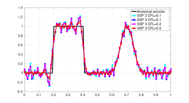
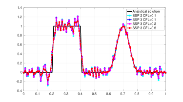
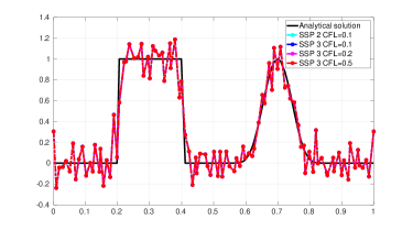
Figure 1. Advection of the initial profile (5.1). Numerical approximations to $u(x,1)=u_{0}(x)$ on meshes with $N=101$ vertices (top: $\zeta=0$, center: $\zeta=0.1$, bottom: $\zeta=0.5$). Space discretization: standard Galerkin. Time stepping and CFL number: see legend.

First, we illustrate the performance of the standard Galerkin method for various time stepping schemes and Courant–Friedrichs–Levi (CFL) numbers $\nu=\Delta t/\min_{i=2,\dots,N}(x_{i}-x_{i-1})$. The results obtained on meshes with perturbation levels $\zeta\in\{0,0.1,0.5\}$ are displayed in Fig. 1. As expected, the presence of steep fronts gives rise to spurious oscillations which can be seen in all curves. The SSP3 time stepping with $\nu=0.5$ seems to produce the least oscillatory results (shown in red) for $\zeta=0$ and $\zeta=0.1$. On the mesh corresponding to the perturbation level $\zeta=0.5$, all Galerkin approximations oscillate strongly even inside the smooth portion of the advected profile. This shows the need for high order stabilization that would prevent global spreading of numerical errors and reduce the amplitude of undershoots/overshoots.

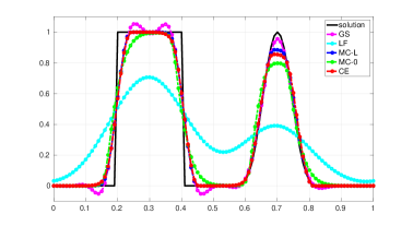
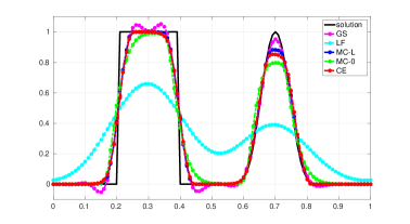
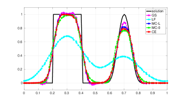
Figure 2. Advection of the initial profile (5.1). Numerical approximations to $u(x,1)=u_{0}(x)$ produced by GS, LF, MC-L, MC-0, and CE on meshes with $N=101$ vertices (top: $\zeta=0$, center: $\zeta=0.1$, bottom: $\zeta=0.5$).

Let us now advect the initial data (5.1) using GS, LF, MC-L, MC-0, and CE on the same meshes. For discretization in time, we use the second order SSP Runge–Kutta method with $\nu=0.25$. The results presented in Fig. 2 illustrate the positive effect of using high order stabilization and flux limiting.

All numerical solutions are free of global oscillations and only the unlimited GS approximation violates maximum principles around discontinuities. Note that this scheme differs from the consistent Galerkin method only in the definition of the time derivatives for the antidiffusive fluxes (3.8). A direct comparison of the two methods (purple curves in Fig. 2 vs. curves in Fig. 1) confirms that the use of low order time derivatives leads to a better target scheme for algebraic flux correction. The low order method introduces enormous amounts of numerical dissipation, while the MC-0 solution profiles are non-symmetric and/or quite diffusive compared to MC-L and CE. The disappointing performance of MC-0 is caused by the failure to compensate the mass lumping error. The best result was delivered by the MC-L scheme, which we found to satisfy the coercivity condition (3.16) on all meshes in this study. The new CE limiting procedure produced $\dot{\alpha}^{\pm}=1$ in all simulation runs, i.e., no coercivity corrections were performed. The resulting approximation is almost indistinguishable from the MC-L solution at discontinuities and only slightly more diffusive in the smooth region. The marginally stronger peak clipping effects are caused by minmod prelimiting for the fluxes $\dot{}f_{ij}$. Without this prelimiting, CE is equivalent to MC-L in the case $\dot{\alpha}^{\pm}=1$.

5.2. Convergence rates for smooth solutions

In the next example, the domain $\Omega=(0,1)$ has an inflow at $x=0$ and an outflow at $x=1$. We use $u^{\textup{in}}=0$ and the $C^{1}(\Omega)$ initial data

$$u_{0}(x)=\begin{cases}\frac{1}{2}\left(1+\cos\left(\frac{\pi}{0.15}(x-0.25)\right)\right)&\mbox{if }|x-0.25|\leq 0.15,\\ 0&\mbox{otherwise}.\end{cases}$$ (5.2)

Note that the analytical solution to this problem has the $H^{2}(\Omega)$ regularity, precisely as required in Theorem 4.2.

We solve this problem on a hierarchy of meshes generated via uniform subdivision of (possibly perturbed) coarse ones. The second order SSP Runge–Kutta method and the CFL number $\nu=0.25$ are employed in each simulation. At the final time $T=0.5$, we compute the $L^{2}(\Omega)$ error, as well as the experimental order of convergence (EOC). The results of grid convergence studies are reported in Tables 3, 3 and 3.

$N$	GC	EOC	GS	EOC	LF	EOC	MC-L	EOC	MC-0	EOC	CE	EOC
33	9.87E-03		4.62E-02		1.93E-01		6.32E-02		8.77E-02		7.82E-02
65	3.12E-03	1.66	1.03E-02	2.16	1.46E-01	0.40	1.42E-02	2.15	3.08E-02	1.51	2.02E-02	1.95
129	9.08E-04	1.78	2.25E-03	2.19	9.94E-02	0.56	3.47E-03	2.04	1.27E-02	1.27	5.33E-03	1.93
257	2.87E-04	1.66	5.44E-04	2.05	6.09E-02	0.71	8.81E-04	1.98	4.17E-03	1.61	1.37E-03	1.95
513	1.60E-04	0.84	1.41E-04	1.94	3.45E-02	0.82	2.24E-04	1.98	1.30E-03	1.68	3.48E-04	1.98

Table 1. Advection of the initial profile (5.2). The $\|\cdot\|_{L^{2}(\Omega)}$ errors at $T=0.5$ and corresponding EOCs on successively refined uniform meshes ($\zeta=0$).

$N$	GC	EOC	GS	EOC	LF	EOC	MC-L	EOC	MC-0	EOC	CE	EOC
33	1.13E-02		4.75E-02		1.93E-01		6.39E-02		8.82E-02		7.88E-02
65	3.02E-03	1.91	1.17E-02	2.02	1.47E-01	0.40	1.52E-02	2.07	3.14E-02	1.49	2.10E-02	1.91
129	7.66E-04	1.98	2.55E-03	2.20	9.99E-02	0.55	3.61E-03	2.07	1.32E-02	1.25	5.54E-03	1.92
257	2.14E-04	1.84	6.03E-04	2.08	6.14E-02	0.70	9.14E-04	1.98	4.32E-03	1.61	1.45E-03	1.93
513	8.08E-05	1.41	1.53E-04	1.98	3.48E-02	0.82	2.32E-04	1.98	1.36E-03	1.67	3.70E-04	1.97

Table 2. Advection of the initial profile (5.2). The $\|\cdot\|_{L^{2}(\Omega)}$ errors at $T=0.5$ and corresponding EOCs on successively refined perturbed meshes ($\zeta=0.1$).

$N$	GC	EOC	GS	EOC	LF	EOC	MC-L	EOC	MC-0	EOC	CE	EOC
33	4.28E-02		7.10E-02		1.98E-01		9.30E-02		1.07E-01		1.05E-01
65	8.31E-03	2.37	2.99E-02	1.25	1.55E-01	0.35	3.77E-02	1.30	4.53E-02	1.23	4.30E-02	1.29
129	1.95E-03	2.09	7.71E-03	1.95	1.09E-01	0.51	9.25E-03	2.03	1.77E-02	1.36	1.09E-02	1.98
257	4.71E-04	2.05	1.91E-03	2.02	6.90E-02	0.66	2.33E-03	1.99	6.02E-03	1.55	2.82E-03	1.95
513	4.99E-04	-0.08	4.82E-04	1.98	3.99E-02	0.79	5.79E-04	2.01	1.90E-03	1.66	7.05E-04	2.00

Table 3. Advection of the initial profile (5.2). The $\|\cdot\|_{L^{2}(\Omega)}$ errors at $T=0.5$ and corresponding EOCs on successively refined perturbed meshes ($\zeta=0.5$).

The failure of GC to converge properly can be blamed on the use of time steps that are too large for this approach. If $\nu$ is set to $0.1$, we observe second order convergence for GC on all meshes employed in this study. All other EOCs are at least as high as the theory predicts. The assumptions of Theorem 4.2 are always satisfied for the LF method (because all correction factors are set to zero), for the MC-0 scheme (because the generalized coercivity condition holds trivially), and for the CE version which is designed to enforce (3.16) in the process of flux correction. If condition (3.16) holds for the GS or MC-L fluxes without additional limiting, Theorem 4.2 is applicable as well. In simulations on perturbed meshes, we observed occasional violations of (3.16) for MC-L and the use of $\dot{\alpha}^{\pm}<1$ in the CE version. On uniform meshes, condition (3.16) was never violated for MC-L or CE with $\dot{\alpha}^{\pm}=1$.

The actual convergence rates of all methods under investigation are, in fact, higher than $h^{1/2}$. The EOC of the LF method gradually approaches 1 as the mesh is refined. This is to be expected because LF is equivalent to the first order upwind method for linear advection on uniform 1D meshes. The MCL-0 convergence rates stagnate around 1.67, while GS, MC-L, and CE exhibit second order convergence already on coarse meshes. Since a locally bound-preserving scheme can be at most second order accurate [33], the behavior of MC-L and CE is optimal. The lack of second order superconvergence for MC-0 can again be attributed to numerical dispersion due to mass lumping.

The fact that some EOCs in Tables 3, 3 and 3 are significantly higher than the provable order $\frac{1}{2}$ is not surprising, since we have not made any assumptions on the choice of correction factors $\alpha_{ij}$ other than condition 3.16. In fact, first order convergence could be shown under the assumption that the overall correction factors, defined by

$$\alpha(u_{h}) =1-\frac{d_{h}(u_{h};u_{h},u_{h})}{\sum_{i=1}^{N}\sum_{j=1}^{i-1}d_{ij}(u_{i}-u_{j})^{2}},$$ (5.3)

$$\dot{\alpha}(u_{h}) =\frac{m_{h}(u_{h};\dot{u}_{h},\dot{u}_{h})}{\sum_{i=1}^{N}\sum_{j=1}^{i-1}m_{ij}(\dot{u}_{i}-\dot{u}_{j})^{2}},$$ (5.4)

behave as $O(h)$. If this is the case, we can gain an additional power of $h$ after applying Young’s inequality in the proof of Theorem 4.2. Similarly to the generalized coercivity condition, it is easy to verify the validity of (5.3) and (5.4) a posteriori. However, it is not so easy to enforce these conditions if they are violated, because this may require undesirable relaxation of local bounds. Moreover, the $O(h)$ behavior of $\alpha(u_{h})$ and $\dot{\alpha}(u_{h})$ cannot be guaranteed for arbitrary $u_{h}\in V_{h}$. Nevertheless, the fact that the EOC of many AFC schemes can be as high as 2 in practice justifies the quest for new limiting criteria and procedures that provably guarantee at least first order convergence for hyperbolic problems.

6. Conclusions

The presented research appears to be the first theoretical investigation of semi-discrete AFC schemes for evolutionary hyperbolic problems. To obtain an a priori error estimate with convergence rate $\frac{1}{2}$, we formulated a generalized coercivity condition and enforced it using a modification of the monolithic convex limiting procedure. As shown numerically, coercivity enforcement has no appreciable negative impact on the accuracy of flux-corrected finite element approximations. Moreover, our numerical examples indicate that the original MCL scheme is essentially coercive if the antidiffusive fluxes are stabilized, e.g., using a low order approximation to the nodal time derivatives.

Of course, the implications of generalized coercivity conditions and performance of limiting procedures based on such conditions require additional numerical studies in the multidimensional case. Furthermore, it is worth investigating if raw antidiffusive fluxes can be stabilized in such a way that coercivity corrections become unnecessary.

It is hoped that the ideas presented in this work can be used for analysis of fully discrete problems and extended to nonlinear conservation laws, hopefully even systems like the Euler equations. Other interesting avenues to explore in future studies include analysis of AFC schemes for other target discretizations, such as discontinuous Galerkin methods and/or higher order finite elements. Moreover, the aspects of inexact numerical integration may need to be taken into account. We invite the interested reader to participate in these research endeavors.

References

• [1] R. Anderson, V. Dobrev, T. Kolev, D. Kuzmin, M. Quezada de Luna, R. Rieben, V. Tomov (2017) High-order local maximum principle preserving (MPP) discontinuous Galerkin finite element method for the transport equation J. Comput. Phys. 334: 102–124 doi: 10.1016/j.jcp.2016.12.031
• [2] G. R. Barrenechea, E. Burman, F. Karakatsani (2017) Edge-based nonlinear diffusion for finite element approximations of convection–diffusion equations and its relation to algebraic flux-correction schemes Numer. Math. 135: 521–545 doi: 10.1007/s00211-016-0808-z
• [3] G. R. Barrenechea, V. John, P. Knobloch (2016) Analysis of algebraic flux correction schemes SIAM J. Numer. Anal. 54: 2427–2451 doi: 10.1137/15M1018216
• [4] G. R. Barrenechea, V. John, P. Knobloch, R. Rankin (2018) A unified analysis of algebraic flux correction schemes for convection–diffusion equations SeMA Journal 75: 655–685 doi: 10.1007/s40324-018-0160-6
• [5] D. A. Di Pietro, A. Ern (2012) Mathematical Aspects of Discontinuous Galerkin Methods Springer doi: 10.1007/978-3-642-22980-0
• [6] A. Ern, J.-L. Guermond (2004) Theory and Practice of Finite Elements Springer doi: 10.1007/978-1-4757-4355-5
• [7] J.-L. Guermond, B. Popov (2016) Invariant domains and first-order continuous finite element approximation for hyperbolic systems SIAM J. Numer. Anal. 54: 2466–2489 doi: 10.1137/16M1074291
• [8] H. Hajduk (2021) Monolithic convex limiting in discontinuous Galerkin discretizations of hyperbolic conservation laws Comput. Math. Appl. 87: 120–138 doi: 10.1016/j.camwa.2021.02.012
• [9] A. Jameson (1993) Computational algorithms for aerodynamic analysis and design Appl. Numer. Math. 13: 383–422 doi: 10.1016/0168-9274(93)90096-A
• [10] A. Jameson (1995) Positive schemes and shock modelling for compressible flows Int. J. Numer. Meth. Fl. 20: 743–776 doi: 10.1002/fld.1650200805
• [11] A. Jameson, W. Schmidt, E. Turkel (1981) Numerical solution of the Euler equations by finite volume methods using Runge–Kutta time stepping schemes AIAA Paper 81-1259 doi: 10.2514/6.1981-1259
• [12] A. Jha, N. Ahmed (2021) Analysis of Flux Corrected Transport Schemes for Evolutionary Convection-Diffusion-Reaction Equations preprint: arXiv:2103.04776
• [13] A. Jha, V. John (2019) A study of solvers for nonlinear AFC discretizations of convection–diffusion equations Comput. Math. Appl. 78: 3117–3138 doi: 10.1016/j.camwa.2019.04.020
• [14] Y. Jiang, H. Liu (2018) Invariant-region-preserving DG methods for multi-dimensional hyperbolic conservation law systems, with an application to compressible Euler equations J. Comput. Phys. 373: 385–409 doi: 10.1016/j.jcp.2018.03.004
• [15] P. Knabner, L. Angermann (2003) Numerical Methods for Elliptic and Parabolic Partial Differential Equations Springer doi: 10.1007/b97419
• [16] V. Kučera, C.-W. Shu (2018) On the time growth of the error of the DG method for advective problems IMA J. Numer. Anal. 39: 687–712 doi: 10.1093/imanum/dry013
• [17] D. Kuzmin (2001) Positive finite element schemes based on the flux-corrected transport procedure in Computational Fluid and Solid Mechanics 887–888 Citeseer
• [18] D. Kuzmin (2009) Explicit and implicit FEM-FCT algorithms with flux linearization J. Comput. Phys. 228: 2517–2534 doi: 10.1016/j.jcp.2008.12.011
• [19] D. Kuzmin (2012) Algebraic flux correction I. Scalar conservation laws in Flux-Corrected Transport 145–192 Springer doi: 10.1007/978-94-007-4038-9_6
• [20] D. Kuzmin (2020) Gradient-based limiting and stabilization of continuous Galerkin methods in Numerical Methods for Flows 331–339 Springer doi: 10.1007/978-3-030-30705-9_29
• [21] D. Kuzmin (2020) Monolithic convex limiting for continuous finite element discretizations of hyperbolic conservation laws Comput. Method. Appl. M. 361: 112804 doi: 10.1016/j.cma.2019.112804
• [22] D. Kuzmin, M. Möller, J. N. Shadid, M. Shashkov (2010) Failsafe flux limiting and constrained data projections for equations of gas dynamics J. Comput. Phys. 229: 8766–8779 doi: 10.1016/j.jcp.2010.08.009
• [23] D. Kuzmin, M. Quezada de Luna (2020) Entropy conservation property and entropy stabilization of high-order continuous Galerkin approximations to scalar conservation laws Comput. Fluids 213: 104742 doi: 10.1016/j.compfluid.2020.104742
• [24] D. Kuzmin, S. Turek (2002) Flux correction tools for finite elements J. Comput. Phys. 175: 525–558 doi: 10.1006/jcph.2001.6955
• [25] C. Lohmann (2019) Physics-Compatible Finite Element Methods for Scalar and Tensorial Advection Problems Springer Spektrum doi: 10.1007/978-3-658-27737-6
• [26] C. Lohmann, D. Kuzmin, J. N. Shadid, S. Mabuza (2017) Flux-corrected transport algorithms for continuous Galerkin methods based on high order Bernstein finite elements J. Comput. Phys. 344: 151–186 doi: 10.1016/j.jcp.2017.04.059
• [27] R. Löhner (2008) Applied Computational Fluid Dynamics Techniques: An Introduction Based on Finite Element Methods John Wiley & Sons (2nd ed.) doi: 10.1002/9780470989746
• [28] K. Mer (1998) Variational analysis of a mixed element/volume scheme with fourth-order viscosity on general triangulations Comput. Methods Appl. Mech. Engrg. 153: 45–62 doi: 10.1016/S0045-7825(97)00064-9
• [29] W. Pazner (2020) Sparse invariant domain preserving discontinuous Galerkin methods with subcell convex limiting preprint: arXiv:2004.08503
• [30] A. Quarteroni, A. Valli (1994) Numerical Approximation of Partial Differential Equations Springer doi: 10.1007/978-3-540-85268-1
• [31] A. Rupp, M. Hauck, V. Aizinger (2020) A subcell-enriched Galerkin method for advection problems URL https://arxiv.org/abs/2006.09041
• [32] V. Selmin (1993) The node-centred finite volume approach: Bridge between finite differences and finite elements Comput. Methods Appl. Mech. Engrg. 102: 107–138 doi: 10.1016/0045-7825(93)90143-L
• [33] X. Zhang, C.-W. Shu (2011) Maximum-principle-satisfying and positivity-preserving high-order schemes for conservation laws: survey and new developments Proc. R. Soc. A 467: 2752–2776 doi: 10.1098/rspa.2011.0153