An Efficient Algorithm for Deep Stochastic Contextual Bandits

Abstract

In stochastic contextual bandit (SCB) problems, an agent selects an action based on certain observed context to maximize the cumulative reward over iterations. Recently there have been a few studies using a deep neural network (DNN) to predict the expected reward for an action, and the DNN is trained by a stochastic gradient based method. However, convergence analysis has been greatly ignored to examine whether and where these methods converge. In this work, we formulate the SCB that uses a DNN reward function as a non-convex stochastic optimization problem, and design a stage-wise stochastic gradient descent algorithm to optimize the problem and determine the action policy. We prove that with high probability, the action sequence chosen by this algorithm converges to a greedy action policy respecting a local optimal reward function. Extensive experiments have been performed to demonstrate the effectiveness and efficiency of the proposed algorithm on multiple real-world datasets.

Introduction

The multi-armed bandit is an interactive machine learning problem and has received tremendous research interest for decades, e.g., (Auer, Cesabianchi, and Fischer 2002; Filippi et al. 2010; Gopalan, Mannor, and Mansour 2014). The stochastic contextual bandit (SCB) problems contain a sequence of rounds $t$, where the agent observes a context $d_{t}\in\mathbb{R}^{n_{d}}$ (for $n_{d}\in I$) which consists of features about all actions and can be regarded as a sample from an unknown distribution that is fixed when shifted in time, e.g., user information in news recommendation system (Li et al. 2010). Then the agent selects an action $a_{t}$ from $K$ choices (e.g., $K$-arms) to get the reward $r_{d_{t},a_{t}}\in[0,1]$, which is i.i.d. drawn from an unknown but fixed distribution with the expectation modeled by the reward function defined below.

Definition 1 (Reward Function)

There exists a real-valued vector $x^{*}\in\mathbb{R}^{n_{x}}$ and a reward function $f(d;x^{*})$ s.t. for all actions $a_{t}\in\{1,2,...,K\}$ and context $d_{t}\sim\mathcal{D}$,

$$\textstyle\mathbb{E}_{r_{d_{t},a_{t}}}[r_{d_{t},a_{t}}\,|\,d_{t},a_{t}]=f_{a_{t}}(d_{t};x^{*}),$$ (1)

where $f_{a_{t}}(d_{t};x^{*})\in[0,1]$ is the $a_{t}^{th}$ output of $f(d_{t};x^{*}).$

Note that the context $d$ can be continuous but there are discrete and a finite number ($K$) of actions. The agent’s goal is to minimize the cumulative regret

$$\textstyle\sum_{t=1}^{T}\mathbb{E}_{r_{d,a}}[r_{d_{t},a^{*}_{d_{t}}}|d_{t},a^{*}_{d_{t}}]-r_{d_{t},a_{t}},$$ (2)

where $T$ is the total number of rounds, and $a_{d_{t}}^{*}$ is the optimal action that maximizes the expected reward $\mathbb{E}_{r_{d,a}}[r_{d,a}|d,a]$.

To minimize the cumulative regret, the agent needs to balance between selecting potentially optimal action to learn its reward distribution (Exploration) and choosing the action with the highest estimated expected reward (Exploitation), a.k.a. the $Exploration\ vs.\ Exploitation$. Earlier studies on SCB problems focus on SCB with a linear reward function, which has been well understood both theoretically and empirically (Auer 2002; Dani, Hayes, and Kakade 2008; Foster et al. 2018; Liu et al. 2018). However, the assumption of a linear reward function may not be satisfied for many real-life problems. Later, many research efforts have been devoted to SCB with a more relaxed assumption on the reward function. In particular, SCB with a deep neural network (DNN) modeled reward function or called deep SCB have attracted great interest, because of the DNN’s powerful expressiveness for complicated real-world problems (Allesiardo, Féraud, and Bouneffouf 2014; Collier and Llorens 2018; Zhou, Li, and Gu 2020; Kveton et al. 2020).

For deep SCB, one may naturally adopt adaptive action policies, which have been successfully employed in SCB with a simple reward function, e.g., a linear or generalized linear reward function. In such policies, the exploration schedule can be dynamically updated based on the observed contexts, selected actions and received rewards in previous rounds. Then the computational complexity generally depends on the dimensionality of the learnable parameters and the contexts, which, however, are often very high for DNNs (because of its power in modeling high-dimensional data). Therefore, it is still not clear how to use adaptive action policies for DNN based on SCB in an efficient way to enable its scalability to large DNNs. For example, recently (Zhou, Li, and Gu 2020) designed a powerful adaptive action policy for deep SCB, but the complicated matrix calculations to update the action policy still make it applicable to small DNNs.

Moreover, although almost all deep SCB algorithms train the DNN-realized reward function with stochastic gradient based methods, rigorous analysis has seldom been given to examine whether and where the DNN and the action policy converge. That is, there is no guarantee that these deep SCB algorithms can learn a stable reward function or effective action policy. Recently (Sokolov et al. 2016b) showed that parameters in the DNN converge to a stationary point, but it remains open to examine the quality of the converged reward function and convergence of the action policy.

Contributions. We propose a stage-wise stochastic gradient descent (SGD) for SCB (SSGD-SCB), which exploits adaptive action policies in an efficient manner and enjoys provable convergence on the action policy $\pi$ and reward function $f$. Our main results are summarized as follows.

• We design an efficient adaptive action policy for deep SCB by dividing contexts into sub-regions, and counting and exploiting how many times an action has been chosen within each sub-region. We then devise a stage-wise SGD method to train the DNN. In this way, the adaptive action policy in SSGD-SCB can be updated incrementally rather than from full history records, and thus does not require complicated matrix calculations, such as those in (Zhou, Li, and Gu 2020; Kveton et al. 2020), so it can be scalable to large DNNs.

• For ease of theoretical analysis, we relax SCB to a non-convex stochastic optimization problem, in which the adaptive action policy makes the variance of the stochastic gradients grow along the rounds. It thus motivates us to stage-wisely reduce the learning rate to account for the growing variance of stochastic gradients. We prove that SSGD-SCB can find a local minimizer under mild regularity conditions, corresponding to a local optimal reward function. The action policy converges to a greedy policy observing the local optimal reward function with high probability. If a stronger condition is assumed for the objective function, we prove that the action policy converges to one which is within an $\epsilon$-neighborhood of the global optimal action policy.

• We have performed extensive experiments to confirm that SSGD-SCB achieves the best cumulative regret compared with state-of-the-art algorithms, and its fitted reward function has the best generalization performance.

Related Work. The agent in SCB can establish and operate on different forms of reward functions, including linear functions and nonlinear functions represented by DNNs. The upper confidence bound (UCB) algorithm (Auer, Cesabianchi, and Fischer 2002) was first applied to the contextual bandit problem with a linear reward function in LINREL(Auer 2002). Since then, many efficient ordinary linear algorithms have been proposed (Dani, Hayes, and Kakade 2008; Chu et al. 2011; Agrawal and Goyal 2013; Agarwal et al. 2014; Foster et al. 2018), and the linear reward functions are also extended to generalized linear models (GLMs) (Li, Lu, and Zhou 2017; Jun et al. 2017; Abeille, Lazaric et al. 2017; Kveton et al. 2019). Some of these algorithms, called agnostic algorithms (Agarwal et al. 2014; Foster et al. 2018), solved the SCB problem by converting it into an optimization problem that can be effectively solved by an existing optimization oracle (solver). However, for SCB problems that correspond to difficult-to-solve optimization problems, new optimization oracles are needed.

Compared with linear and generalized linear models, DNN is more powerful to fit the high dimensional context such as images or board configurations of board games. DNNs have been used to find a low-dimension representation of the raw context for SCB algorithms with a linear reward function (Liu et al. 2018; Riquelme, Tucker, and Snoek 2018). DNNs have also been used to directly represent the expected reward function to result in deep SCB methods (Allesiardo, Féraud, and Bouneffouf 2014; Collier and Llorens 2018; Zhou, Li, and Gu 2020; Kveton et al. 2020). For deep SCB, there have been static action policies such as the $\epsilon$-greedy policy in NeuralBandit1 (Allesiardo, Féraud, and Bouneffouf 2014) and noise-added greedy policy in DeepFPL (Kveton et al. 2020). In these policies, the calculation of action distribution (as a policy) is independent of the information collected in previous rounds. Recently (Zhou, Li, and Gu 2020) proposed an adaptive action policy for deep SCB, but it suffers high computational complexity. Based on full gradients, a convergence analysis was given by presenting an upper bound on the expected cumulative regret. In this paper, we analyze the convergence of the proposed method based on stochastic gradients, which is much more practical than full gradients in the training of DNNs.

Organization. The remainder of this paper is structured as follows. In the problem setting section, we formulate the SCB into an optimization problem and then propose SSGD-SCB to solve the optimization problem in the next section. After that, theoretical properties of SSGD-SCB are discussed in the section of theoretical analysis. Finally, we present the experimental results in the section of experiments, and conclude the paper with a brief discussion on the future work in the section of conclusions and future work.

The Problem Formulation

In this section, we formulate an upper bound on the expected cumulative regret which can be optimized by stochastic gradient based methods. All proofs of lemmas and theorems are deferred to the Appendix A.

Notation. We use $\|\cdot\|$ to denote the 2-norm of vectors. The notation $\mathcal{O}(\cdot)$, $\Omega(\cdot)$, $\Theta(\cdot)$ are used to hide constants which do not rely on the setup of the problem parameters and the notation $\tilde{\mathcal{O}}(\cdot)$, $\tilde{\Omega}(\cdot)$, $\tilde{\Theta}(\cdot)$ are used to additionally hide all logarithmic factors. The operator $\mathbb{E}_{x}[\cdot]$ represents taking the expectation over the random variable listed in the subscript, while $\mbox{VAR}_{x}[\cdot]$ calculates the corresponding variance, and $\nabla f(\cdot)$ is the full gradient.

We start from defining an objective function $F(x)$ when feedback for all actions can be observed.

Definition 2 (The Objective Function with Full Feedback)

Suppose that after observing the context $d$, the agent gets all candidate actions’ rewards (i.e., the full feedback). The objective function is

$$\textstyle F(x)=\mathbb{E}_{d}\sum_{a=1}^{K}\mathbb{E}_{r_{d,a}}\big{[}(f_{a}(d;x)-r_{d,a})^{2}|d,a\big{]}.$$

It is calculated as the expected squared error between the estimated action reward and the actual reward $r_{d,a}$. A smaller objective $F(x)$ corresponds to a better estimation of $f(d;x)$. Furthermore, the global minimizer of $F(x)$ corresponds to the $x^{*}$ used in Definition 1, forming the optimal reward function $f(d;x^{*})$. Lemma 1 characterizes this result.

Lemma 1

$x^{*}$ in Eq. (1) is a global minimizer of $F(x)$. With $x=x^{*}$, we have $F(x^{*})=\mathbb{E}_{d}\sum_{a=1}^{K}\mbox{VAR}_{r_{d,a}}[r_{d,a}|d,a]$.

We now establish the connection between the expected cumulative regret Eq.(2) and $F(x)$ in Lemma 2.

Lemma 2

Suppose in the $t^{th}$ round, the agent estimates the reward of actions with $f(d_{t},x_{t})$, where $x_{t}$ is inferred from the history $\mathcal{H}_{t-1}=\{d_{\tau},a_{\tau},r_{d_{\tau},a_{\tau}},\xi_{\tau}|\tau\in\{1,2,...,t-2\}\}$, where $\xi_{\tau}$ is the set of all other information the agent observes at round $\tau$, e.g., random variables used in the action policy. Let $a_{t}^{*}=\arg\max_{a}f_{a}(d_{t},x_{t})$. The expected cumulative regret in Eq. (2) can be upper bounded by

$$\textstyle\sum_{t=1}^{T}Pr(a_{t}\neq a_{t}^{*})+2\sqrt{K}\sum_{t=1}^{T}\mathbb{E}_{\mathcal{H}_{t-1}}\sqrt{F(x_{t})-F(x^{*})}.$$ (3)

In Eq. (3), the first term is the regret incurred due to the exploration of the agent’s action policy and $r_{d,a^{*}}-r_{d,a_{t}}\leq 1$ because $r\in[0,1]$. For example, when the $\epsilon$-greedy policy is used, the probability in this term becomes $\epsilon$. The second term represents the error of the agent’s estimation on the expected action reward measured by $F(x)$ in Definition 2. Thus, minimizing Eq. (2) can be relaxed to minimizing its upper bound, or equivalently $F(x)$. Since the agent can only observe the selected action’s reward at each round, it does not have the full feedback to compute $F(x)$ during the iterative process and thus can only minimize $F(x)$ with $\mathcal{H}_{t-1}$.

The regret produced by the second term heavily relies on the agent’s exploration measured by the first term. For example, if the agent does not conduct much exploration, $F(x_{t})$ can not be efficiently decreased with the unbalanced actions and rewards in the history $\mathcal{H}_{t-1}$. To simplify the interaction between these two terms, we focus on a set of action policies in which actions will be selected with a probability that is bounded in terms of $t$, as shown in Assumption 1.

Assumption 1

At $t\in\{1,2,$ $...,T\}$, for any $d_{t}\sim\mathcal{D}$ and $\mathcal{H}_{t-1}$, $\pi(a_{t}\,|\,d_{t},\mathcal{H}_{t-1})\geq\Omega(\frac{1}{t^{\mathcal{C}}})$, where $\mathcal{C}>0$.

Remark 1

Assumption 1 is a mild assumption because $\pi\geq 0$ is a probability, and this decreasing lower bound approaches $0$ as the number of rounds increases, and it can find a proper constant in $\Omega$ that does not limit the agent’s exploration (the first term in Eq. (3)).

We can then use the Inverse Propensity Scoring (IPS) to build a corrected stochastic gradient ${\tilde{g}}$, as shown in Lemma 3. Thus, we can use SGD methods to decrease $F(x_{t})$ by moving $x_{t-1}$ in the opposite direction of ${\tilde{g}}$.

Lemma 3 (Inverse Propensity Scoring)

At round $t\in\{1,2,$ $...,T\}$, for any $d_{t}\sim\mathcal{D}$, and $a_{t}\in\{1,2,..,,K\}$, the loss for selecting $a_{t}$ is defined as $l_{d_{t},a_{t}}(x{;r_{d_{t},a_{t}}})=(f_{a_{t}}(x;d_{t})-r_{d_{t},a_{t}})^{2}$. Let

$$\textstyle{\tilde{g}}(x;\mathcal{H}_{t})=\frac{1}{\pi(a_{t}|d_{t},\mathcal{H}_{t-1})}\nabla l_{d_{t},a_{t}}(x;r_{d_{t},a_{t}}),$$ (4)

where $\nabla l$ is the gradient of $l$ with respect to $x$. Under Assumption 1, we have that

(1) The stochastic gradient $\tilde{g}$ is an unbiased estimate of the full gradient $\nabla F(x)$, i.e., $\mathbb{E}_{\mathcal{H}_{t}}{\tilde{g}}(x;\mathcal{H}_{t})=\nabla F(x)$.

(2) The element-wise variance of $\tilde{g}$ is upper bounded by $\mathbb{E}_{d_{t}}\sum_{a=1}^{K}\mathbb{E}_{r_{d_{t},a}}t^{\mathcal{C}}\|\nabla l_{d_{t},a}(x;r_{d_{t},a})\|^{2}$.

For notation convenience, we will use $\tilde{g}_{t}(x)$ to represent ${\tilde{g}}(x;\mathcal{H}_{t})$ in the sequel.

Lemma 3 shows that the IPS corrects the stochastic gradient $\nabla l$ by dividing it by $\pi(a_{t}\,|\,d_{t},\mathcal{H}_{t-1})$ to reach an unbiased estimate of $\nabla F(x)$, but this correction step causes the variance of stochastic gradients to approach infinity when $\pi$ goes to $0$ at certain $a$. Specifically, when the SCB shifts from the exploration to exploitation stage, the action policy $\pi$ transits from the initial stage of evenly choosing among actions to later stages of selecting a specific action where the probabilities $\pi$ for other actions approach 0, as shown in Fig. 1. However, for SGD to converge, the variance of stochastic gradient needs to be upper bounded. (Ge et al. 2015; Allen-Zhu 2018). When employing SGD methods to solve SCB, although one may use a fast decaying learning rate to resolve the increasing variance, this could result in a very slow convergence rate (Johnson and Zhang 2013). Therefore, it is unclear how to find a balance between the decaying speed of the learning rate and the drifting speed of action policy from exploration to being greedy.

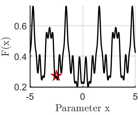
(a)

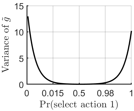
(b)

Figure 1: A simple SCB problem showing the effect of action policy on the variance of IPS corrected stochastic gradient $\tilde{g}$. Here, $\mathcal{D}$ contains two contexts, $d_{1}=2$ and $d_{2}=5$, both are uniformly sampled. In each round, the agent can select either $a_{1}$ or $a_{2}$. The reward of $r_{d_{1},a_{1}}$, $r_{d_{1},a_{2}}$, $r_{d_{2},a_{1}}$ and $r_{d_{2},a_{2}}$ are randomly drawn from $\mbox{unif}(0.2,0.8)$, $\mbox{unif}(0.55,0.85)$, $\mbox{unif}(0.3,0.9)$ and $\mbox{unif}(0,0.2)$ respectively. The reward functions are $f_{a_{1}}(d;x)=0.2sin^{2}(dx)+0.8e^{-(dx)^{2}}$ and $f_{a_{2}}(d;x)=0.8sin^{2}(dx)+0.2e^{-(dx)^{2}}$, where $x\in\mathbb{R}$ is the learnable parameter. (a) $F(x)$ of this model, and the star marks the position used in Fig. 1(b). (b) The variance of $\tilde{g}$ under different $\pi$ (or Pr(selecting $a_{1}$)).

The Proposed Method

In this section, we develop the stage-wise SGD for SCB (SSGD-SCB). Stage-wise SGD has been studied in non-convex optimization and widely used in training DNNs where the step size when moving along a negative stochastic gradient takes multiple values at different stages of the optimization process. The method uses a relatively large learning rate in the first stage, and gradually decays it in subsequent stages. It has been shown that stage-wise SGD helps alleviate the learning-rate-dilemma: a fixed large learning rate is prone to jump out of local minimizer neighborhood while a small learning rate results in very slow convergence (Zhu et al. 2018).

Notations. Before describing the SSGD-SCB method, we define some notations. Let $T_{s}=T_{0}s^{2\upsilon}$ be the number of rounds in the $s^{th}$ stage ($s\in\{1,...,\mathcal{S}\}$) where $T_{0}$ is the initial number of rounds and $\upsilon\in[1,\infty)$ is a hyper-parameter controlling the rate of increasing round numbers along stages. Note that we control $T_{s}$ according to our theoretical analysis in Theorem 1. Let $I(s,n)$ be the total number of rounds that have been performed at the $n^{th}$ rounds of the $s^{th}$ stage.

In every round, SSGD-SCB performs two major tasks: action selection and backpropagation.

1:  Input: The initial point $x_{1}$, the number of rounds $T_{0}$ in the first stage, the noise scale $\mathcal{N}_{0}$, the initial learning rate $\eta_{0}$, and parameters $\omega$ and $C$. According to Remark 4, we set $\upsilon=1$, ,$\beta=\frac{11}{24}$ and $\kappa=0.5$.

2:  for $s=1$ to $\mathcal{S}$ do

3:     $T_{s}=T_{0}s^{2}$

4:     for $n=1$ to $T_{s}$ do

5:        //Action Selection

6:        The context $d_{I(s,n)}$ is revealed

7:        $c_{s,n}=\operatorname*{argmax}_{k}f_{k}(d_{I(s,n)};x_{I(s,n)})$

8:        for $k=1$ to $K$ do

9:           Calculate $\pi(k|d_{I(s,n)},\mathcal{H}_{I(s,n)-1})$

10:        end for

111:        $a_{I(s,n)}\sim\pi(\cdot|d_{I(s,n)},\mathcal{H}_{I(s,n)-1})$

212:        //Backpropagation

313:        $r_{d_{I(s,n)},a_{I(s,n)}}$ is revealed

414:        $N_{I(s,n)+1,a,c_{s,n}}=N_{I(s,n),a,c_{s,n}}+1$

15:        Update $x_{I(s,n)+1}$ using Eq. (8)

16:     end for

17:  end for

Algorithm 1 SSGD-SCB

Action Selection. Here by dividing observed contexts into clusters, we develop an efficient action selection policy which can adapt the exploitation scheme based on how often an action is visited in the cluster which the current context belongs to. As a warm-up, we first present a simple adaptive action policy below:

$$\textstyle W_{s,n,a}=\left\{\begin{aligned} &\textstyle U_{s,n,a},&a=\arg\max_{k}U_{s,n,k};\\ &\textstyle\frac{U_{s,n,a}}{s^{\omega}},&else,\end{aligned}\right.$$ (5)

$$\textstyle\pi_{0}(a\,|\,d_{I(s,n)},\mathcal{H}_{I(s,n)-1})=\frac{0.05}{Ks^{0.5\kappa}}+\frac{(1-\frac{0.05}{s^{0.5\kappa}})W_{s,n,a}}{\sum_{k=1}^{K}W_{s,n,k}},$$

where $U_{s,n,a}=f_{a}(d_{I(s,n)};x_{I(s,n)})$, and $\omega\in(\frac{\kappa}{2},\infty)$ and $\kappa\in(0,\upsilon)$ are tuning parameters. The policy $\pi_{0}$ is a convex combination of the exploration probability $\frac{1}{K}$ and the exploitation probability $W_{s,n,a}/(\sum_{k}W_{s,n,k})$ with a combination coefficient of $0.05s^{-0.5\kappa}$. By this definition, $\pi_{0}$ has a lower bound $\frac{0.05}{Ks^{0.5\kappa}}$ for any action and this lower bound decreases along stages as controlled by $\kappa$ which is a constant. It is easy to check that $\pi_{0}$ satisfies Assumption 1.

When $s$ increases, $\pi_{0}$ will drift from a more even chance of choosing actions to a more greedy policy which selects the action with the largest estimated reward. To shift to choose the action with the largest estimated reward, the parameter $\omega$ controls the weight decay of other actions. Thus, $\pi_{0}$ can dynamically balance the exploration and exploitation. However, if $U_{s,n,a}=f_{a}(d_{I(s,n)};x_{I(s,n)})$, it does not utilize the history of action selection in previous rounds.

Inspired by the effective multi-armed bandit algorithm - UCB1 (Auer, Cesa-Bianchi, and Fischer 2002) that balances exploration and exploitation via the visit number of actions, we form a new exploitation term incorporating the history action visits. We first group observed contexts according to the action that gives the largest reward estimated at the respective round:

$$\textstyle c=\operatorname*{argmax}_{k}f_{k}(d_{t};x_{t}),$$ (6)

so $d_{t}$ belongs to cluster $c$ (as one of the $K$ clusters). Thus, for the current context $d_{I(s,n)}$, which belongs to cluster $c_{s,n}$, we count the number of times, $N_{I(s,n),a,c_{s,n}}$, an action $a$ has been visited before the round $I(s,n)$. We can revise $U_{s,n,a}$ to incorporate $N_{I(s,n),a,c_{s,n}}$ according to Eq. (7). Note that the bookkeeping of $c_{s,n}$ and $N_{I(s,n),a,c_{s,n}}$ is performed iteratively.

$$\textstyle U_{s,n,a}=f_{a}(d_{I(s,n)};x_{I(s,n)})+C\frac{(\sum_{k=1}^{K}N_{I(s,n),k,c_{s,n}})^{\beta}}{\sqrt{N_{I(s,n),a,c_{s,n}}}},$$ (7)

where $\beta\in(0,0.5)$ and $C\in[0,\infty)$ are hyperparameters weighting the action-visit term. Eq. (7) provides a mechanism to adapt the exploitation before becoming completely greedy based only on $f_{a}(d_{I(s,n)};x_{I(s,n)})$. The actions with a smaller visit number will have a greater chance to be explored. At last, we calculate the final action policy $\pi(\cdot|d_{I(s,n)},\mathcal{H}_{I(s,n)-1})$ with the new $U_{s,n,a}$ in Eq. (5). Algorithm 1 summarizes all the steps. If there exists an action that has been visited less than a threshold, frequently visited actions will only be selected with low probability until the visit numbers of all actions pass the threshold. Formal descriptions are given in Lemma 4 (see Appendix A for the proof).

Lemma 4

For a cluster $c_{s,n}$, if there exists an action with its visit number smaller than $\frac{C^{2}(\sum_{k=1}^{K}N_{I(s,n),k,c_{s,n}})^{2\beta}}{C^{2}K+2C\sqrt{K}+1}$, the action with the largest visit number will be selected by $\pi$ with probability $\mathcal{O}(s^{-0.5\kappa})$, while the action with the largest $U_{s,n,a}$ will be selected with probability greater than $\frac{(1-0.05s^{-0.5\kappa})s^{\omega}}{s^{\omega}+K-1}$.

Backpropagation. In the $n^{th}$ round of $s^{th}$ stage, after taking the action $a_{I(s,n)}$, the agent observes the corresponding reward $r_{d_{I(s,n)},a_{I(s,n)}}$. SSGD-SCB then updates its parameters as follows. First, the visit count of $a_{I(s,n)}$ is increased by one. Then the stochastic gradient $\tilde{g}_{I(s,n)}(x_{I(s,n)})$ is computed based on the context $d_{I(s,n)}$, the reward $r_{d_{I(s,n)},a_{I(s,n)}}$, and $\pi(a|d_{I(s,n)},\mathcal{H}_{I(s,n)-1})$ in Eq. (4). Finally,the parameters $x_{I(s,n)}$ can be updated in a SGD step:

$$\textstyle x_{I(s,n)+1}=x_{I(s,n)}-\eta_{s}(\tilde{g}_{I(s,n)}(x_{I(s,n)})+\mathcal{N}_{s}),$$ (8)

where $\eta_{s}=\frac{\eta_{0}}{s^{\upsilon}}$ is the learning rate decaying from initial $\eta_{0}$, and $\mathcal{N}_{s}=\frac{s^{\frac{\kappa}{2}}\mathcal{N}_{0}w}{\|w\|}$ is a noise term where $w$ is a vector of noise drawn from standard Gaussian and $\mathcal{N}_{0}$ is a hyper-parameter controlling the magnitude of noise. Since $\kappa<\upsilon$ (see Eq.(5)), $\eta$ decays faster than the growth of the variance of stochastic gradients over rounds. Because our optimization problem is non-convex, there can be saddle points (i.e., $\nabla F(x)=0$, but $x$ is not a local extremum). Prior work (Ge et al. 2015) has informed that adding proper noise to the stochastic gradient can help escape from strict saddles. The noise needs to be small enough without incurring a sharp increase in the variance of gradients, which we prove that the variance caused by this noise is smaller than that due to dividing by $\pi$. The noise $\mathcal{N}_{s}=\Theta(s^{\frac{\kappa}{2}})$ increases along stages because if a fixed small noise is used, it will be hard in later stages to escape strict saddles when $\eta_{s}$ is very small.

Theoretical Analysis

When the reward function $f$ is represented by a DNN, the objective $F(x)$ is non-convex. It is NP-hard to find a global minimizer of a non-convex problem or even to approximate a global minimizer (Jain and Kar 2017), especially when we cannot assume properties such as PL-condition (Yuan et al. 2019) or $\sigma$-Nice condition (Hazan, Levy, and Shalev-Shwartz 2016) (for which an approximate optimal solution can be found in polynomial time). Under mild conditions, the SGD method can be proved to reach just a stationary point for non-convex optimization.

Given that SCB is not only non-convex but also a stochastic optimization process, it becomes even more challenging to analyze convergence, so it has hardly seen any prior work discussing where SCB algorithms converge. Under four assumptions (see below), we prove that SSGD-SCB can find a local minimizer of $F(x)$, corresponding to a suboptimal reward function $f$ and a sub-linear expected local cumulative regret. Before introducing the concept of local cumulative regret, we first give our Assumption 2 on $F(x)$. Then we define the local optimal convergence used in the subsequent analysis in Definition 4.

Definition 3 ($(\alpha,\gamma,\epsilon,\delta)$-Strict Saddle)

A twice differentiable function $\mathcal{F}(x)$ is $(\alpha,\gamma,\epsilon,\delta)$-strict saddle, if for any point $x$, at least one of the following conditions is true:
1. $\|\nabla\mathcal{F}(x)\|\geq\epsilon$.
2. The minimum eigenvalue of $\nabla^{2}\mathcal{F}(x)$ is smaller than a fixed negative real number $\gamma$.
3. There is a local minimizer $x^{l}$ such that $\|x-x^{l}\|\leq\delta$, and the function $\mathcal{F}(x^{\prime})$ restricted to $2\delta$ neighborhood of $x^{l}$ ($\|x^{\prime}-x^{l}\|\leq 2\delta$) is $\alpha$-strongly convex (see Appendix for definition).

Assumption 2 ((Ge et al. 2015))

The objective function with full feedback, $F(x)$, is an L-smooth, bounded, $(\alpha,\gamma,\epsilon,\delta)$-strict saddle function, and has $\rho$-Lipschitz Hessian (see Appendix for definition).

Definition 4

Let $t^{\prime}$ be a fixed round number. The event of local optimal convergence can be defined as $\mathfrak{E}^{t^{\prime}}=\{$With $\mathcal{L}>0$, for any round $t>t^{\prime}$ and any history $\mathcal{H}_{t^{\prime}}$, there exists a local minimum of $F(x)$ marked as $x^{\mathcal{H}_{t^{\prime}}}$ such that $\|x_{t}-x^{\mathcal{H}_{t^{\prime}}}\|\leq\tilde{\mathcal{O}}(\frac{1}{t^{\mathcal{L}}})\leq\delta\}$.

For a deterministic optimization problem, one may argue that a method converges to any local minimum. For SCB, Definition 4 is more strict because it does not allow $x$ to jump among different local minimums over the stochastic process after a certain number of rounds is reached. Because of the stochasticity of stochastic gradients, this is difficult to guarantee (Kleinberg, Li, and Yuan 2018). Conditioned on $\mathfrak{E}^{t^{\prime}}$, $\sqrt{F(x_{t})-F(x^{*})}$ in Eq. (3) can be upper bounded by $\sqrt{|F(x_{t})-F(x^{\mathcal{H}_{t^{\prime}}})|}+\sqrt{F(x^{\mathcal{H}_{t^{\prime}}})-F(x^{*})}$. The second term of this upper bound measures the regret produced by the difference between the loss of local and global minimizers. This difference is inaccessible to the agent, and thus we focus on examining the local cumulative regret:

$$\textstyle\sum_{t=1}^{T}\big{[}Pr(a_{t}\neq a_{t}^{*})+\mathbb{E}_{\mathcal{H}_{t-1}}2\sqrt{K|F(x_{t})-F(x^{\mathcal{H}_{t^{\prime}}})|}\big{]}.$$

The local cumulative regret measures the transition speed of the action policy from exploration to exploitation (the first term) and the convergence rate of the current loss to the local optimal loss (the second term). With Assumptions 2-4, conditioned on the event $\mathfrak{E}^{t^{\prime}}$, we can show that if the local cumulative regret is sub-linear, the action policy selected by SSGD-SCB approaches (in expectation) to a policy defined by the local optimal reward function over rounds. This is obtained by discussing the expected mismatching rate defined in Definition 5. We show that the mismatching rate has a zero-approaching upper bound, as shown in Lemma 5 (see Appendix B for the proof). As an extension, if $F(x)$ is convex, SSGD-SCB can reach a sub-linear expected cumulative regret by achieving a zero-approaching expected mismatching rate with the optimal policy, as discussed in Remark 3.

Assumption 3

Denote the set of local minimizers of $F(x)$ as $X$. For any $x^{l}\in X$, given any sampled context $d_{t}$, the largest output in $f(d_{t};x^{l})$ is unique. In other words, if $a^{x^{l}}_{d_{t}}=\arg\max_{k\in\{1,2,...,K\}}f_{k}(d_{t};x^{l})$, then $f_{a}(d_{t};x^{l})\neq f_{a^{x^{l}}_{d_{t}}}(d_{t};x^{l})$ for any $a\neq a_{d_{t}}^{x^{l}}$.

Remark 2

Assumption 3 is a variant of the Assumption 3 used in a Thompson Sampling based contextual bandit algorithm (Gopalan, Mannor, and Mansour 2014) which assumes a convex loss function and the largest output in $f(d_{t};x^{*})$ (where $x^{*}$ is a global optimizer) is unique. We deal with a non-convex loss so we assume that the largest reward output for a local minimizer is unique.

Assumption 4 ((Lu, Pál, and Pál 2010))

The gradient of $f$ is bounded. In other words, $\exists M_{f}\in\mathbb{R}_{*}^{+}$ such that $\forall d\sim\mathcal{D}$, $\forall x\sim\mathcal{R}^{n_{x}}$ and $\forall a\in\{1,2,...,K\}$, $\|\nabla f_{a}(x;d)\|\leq\sqrt{M_{f}}$.

Definition 5 (Expected Mismatching Rate)

Let $X$ be the set of local minimizer of a non-convex $F(x)$, the expected local optimal mismatching rate is

$$\textstyle\mathbb{E}_{\mathcal{H}_{T}}\big{[}\min_{x^{l}\in X}(\sum_{t=1}^{T}\frac{\mathbf{1}(a_{d_{t}}\neq a_{d_{t}}^{x^{l}})}{T})\big{]},$$

where $T$ is the total number of rounds, and $a_{d_{t}}^{x^{l}}=\arg\max_{k}(f_{k}(d_{t};x^{l}))$.

Lemma 5

With Assumptions 2-4, conditioned on the event $\mathfrak{E}^{t^{\prime}}$, if the expected local regret is sub-linear, the expected mismatching rate defined in Definition 5 has a zero-approaching upper bound.

Remark 3

If $F(x)$ is a convex function, the expected mismatching rate can be defined for a global minimizer of $F(x)$. The mismatching rate is the upper bound of expected cumulative regret averaged over $T$.

SSGD-SCB for Non-Convex Objectives. We analyze the convergence of SSGD-SCB in two steps. First, based on Assumptions 2 and 5, Theorem 1 characterizes that if the stage number is large enough, $x$ can reach and be captured at a local minimizer with high probability. We then prove convergence of the action policy by examining the mismatching rate in Theorem 2. All proofs are provided in Appendix B.

Assumption 5

for any context d, action a and solution $x$, $\exists M\in\mathbb{R}_{*}^{+}$, $\|\nabla l_{d,a}(x)\|^{2}\leq M^{2}$.

Theorem 1

Under Assumptions 2 and 5, for any $\zeta\in(0,1)$, there exists a large enough stage $s^{\prime}$ such that with probability at least $1-\zeta$, for $\forall s>s^{\prime}$ and $\forall n\in\{1,2,...,T_{0}s^{2\upsilon}\}$, we have $\|x_{I(s,n)}-x^{s^{\prime}}\|^{2}\leq\mathcal{O}(s^{\kappa-\upsilon}\log\frac{1}{\eta_{s}\zeta})\leq\delta$, where $x^{s^{\prime}}$ is a local minimizer of $F(x)$.

With $\mathfrak{E}_{t^{\prime}}$ defined in Definition 4, Theorem 1 shows that $Pr(\mathfrak{E}^{I(s^{\prime},T_{s^{\prime}})})\geq 1-\zeta$. With Assumptions 2-5, conditioned on $\mathfrak{E}^{I(s^{\prime},T_{s^{\prime}})}$, we show that the mismatching rate between the actions taken by SSGD-SCB and the policy defined by a local minimizer $x^{l}$ will converge to 0 as $T\rightarrow\infty$.

Theorem 2

Under Assumptions 2-5, if $\mathcal{S}$ is large enough, with probability at least $1-\zeta$, the expected mismatching rate is bounded as follows:

$$\textstyle\mathbb{E}\big{[}\min_{x^{l}\in X}(\sum_{s=1}^{\mathcal{S}}\sum_{n=1}^{T_{0}s^{2}}\frac{\mathbf{1}(a_{I(s,n)}\neq a^{x^{l}}_{d_{I(s,n)}})}{\sum_{s=1}^{\mathcal{S}}T_{0}s^{2}})\big{]}\leq\tilde{\mathcal{O}}(\frac{1}{\mathcal{S}^{\Lambda}}),$$

where $\Lambda=\min(\frac{\kappa}{2},(1-2\beta)(1+2\upsilon),(2\beta-1)(1+2\upsilon)+\kappa-\upsilon)$.

Remark 4

By setting $\upsilon=1$ and assuming $\frac{\kappa}{2}=(1-2\beta)(1+2\upsilon)=(2\beta-1)(1+2\upsilon)+\kappa-\upsilon$, we can set $\kappa=0.5$, and then $\beta=\frac{11}{24}$ in an implementation of Algorithm 1. Then we have $\Lambda=0.25$. Note that when the exploration parameter $C$ in Eq. (7) equals 0, the upper bound is $\mathcal{O}(\frac{1}{\mathcal{S}^{0.25}})$.

Remark 5

With an additional structural assumption on $F(x)$, i.e. $\sigma$-nice, a variant of SSGD-SCB can achieve a zero approaching expected mismatching rate, in which $X$ is a set of $\epsilon$-optimal solution ($F(x^{l})-F(x^{*})\leq\epsilon$). Besides, if $F(x)$ is a strongly convex function, SSGD-SCB can achieve a sub-linear expected cumulative regret. These two cases are discussed in Appendices E and F.

Experiments

We have performed extensive experiments to confirm the effectiveness and computational efficiency of the proposed method, SSGD-SCB with a DNN reward function. Another set of experiments have also been conducted for SSGD-SCB with a linear reward function.

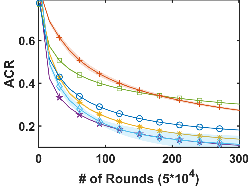
(a) ACR on CIFAR-10

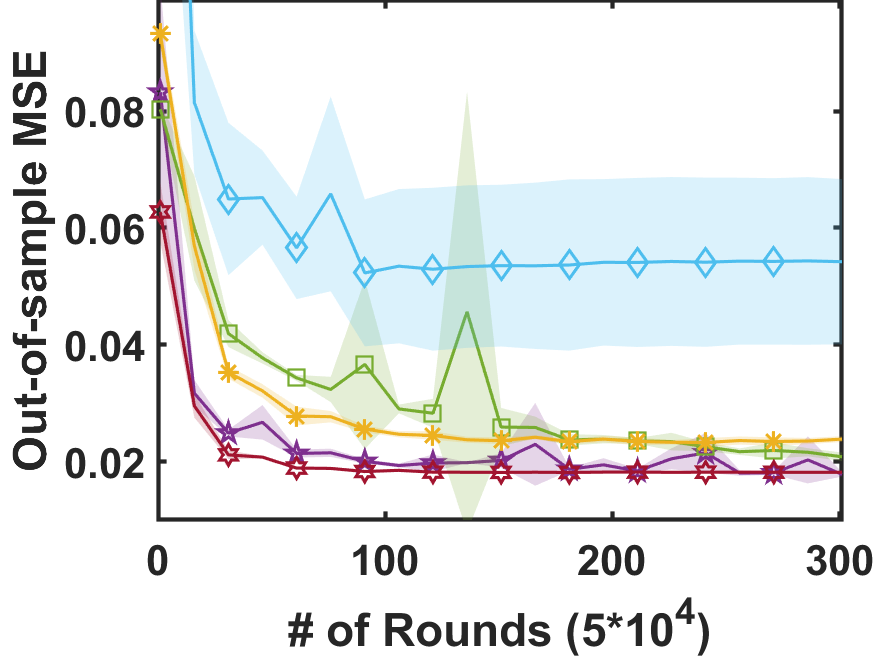
(b) Out-of-sample MSE on CIFAR-10

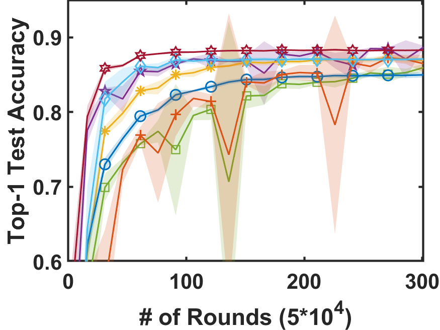
(c) Top-1 test accuracy on CIFAR-10

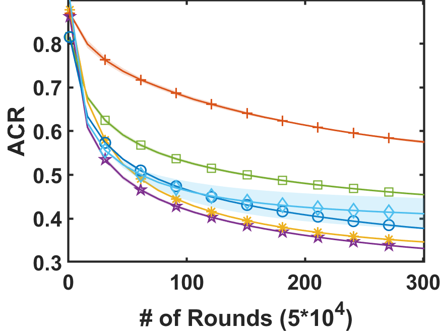
(d) ACR on CIFAR-10+N

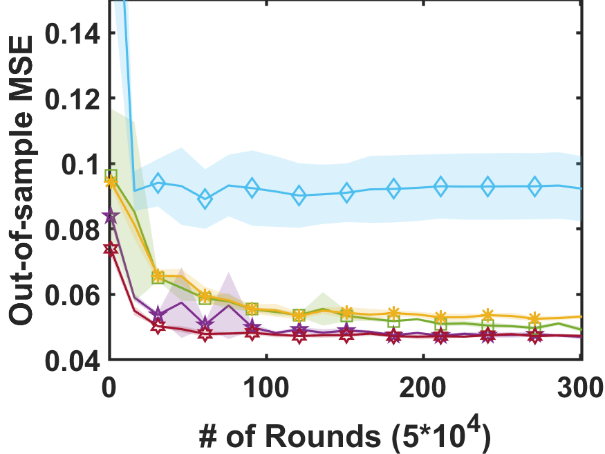
(e) Out-of-sample MSE on CIFAR-10+N

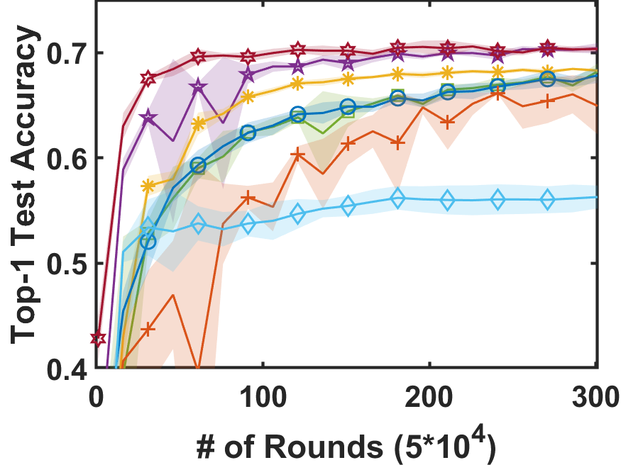
(f) Top-1 test accuracy on CIFAR-10+N

Figure 2: Average cumulative regret, out-of-sample MSE and top-1 test accuracy of SSGD-SCB on CIFAR-10 and CIFAR-10+N. EL and CE have no out-of-sample MSE because rather than fitting rewards of actions, they learn action policy directly.

Datasets. We use the CIFAR-10 dataset (Simonyan and Zisserman 2014), which has been widely used for benchmarking non-convex optimization algorithms. It consists of $60K$ $32\times 32$ RGB images from $10$ classes. Considering that it does not include noise in the image label, we construct a noise-added version of CIFAR-10, called CIFAR-10+N, by correctly marking the labels of 80% samples while randomly marking the labels of the rest 20% samples. For both CIFAR-10 and CIFAR-10+N data, $50K$ samples are selected as the training set $D_{train}$ while the rest $10K$ samples form the test set $D_{test}$.

Experimental Methods. At each round $t$, an image is randomly sampled from the training set followed by an augmentation with random crop (4$\times$4 region) and horizontal flip to increase its diversity, and then used as the context $d_{t}$. Next, the agent selects an index of class as the selected action $a_{t}$, and then the label corresponding to $a_{t}$ is revealed as the reward $r_{d_{t},a_{t}}$. We denote the $i^{th}$ sample as $(d_{i},l_{i})$, where $d_{i}$ is the $i^{th}$ image and $l_{i}=[l_{i,1},l_{i,2},...,l_{i,K}]^{T}$ is its one-hot encoded label. For simplicity, we use the average cumulative regret (ACR), $1-\frac{\sum_{t=1}^{T}r_{d_{t},a_{t}}}{T}$, as an estimation of the expected cumulative regret. With the test set, we measure the generalization performance of the reward function on the reward of the optimal action and the rewards of all candidate actions, respectively by top-1 test accuracy, $\sum_{(d_{i},l_{i})\in\mathcal{D}_{test}}\frac{l_{i,\arg\max_{k}f_{k}(d_{i};x_{t})}}{|D_{test}|}$ and the out-of-sample min-squared error (MSE), $\sum_{(d_{i},l_{i})\in D_{test}}\frac{\|f(d_{i};x_{t})-l_{i}\|^{2}}{K|D_{test}|}$.

Baseline Algorithms. We compared SSGD-SCB with a DNN realized reward function against five baseline algorithms: (1) $\epsilon$-greedy policy, a basic SCB algorithm where the agent selects actions, either greedily with probability $1-\epsilon$ or randomly with probability $\epsilon$; (2 and 3) Bandit structured prediction with Expected Loss (EL) and Cross-Entropy (CE) minimizations (Sokolov et al. 2016a), originally used in the field of interactive Natural Language Processing; (4) Neural Linear (NL) (Riquelme, Tucker, and Snoek 2018), which learns the action policy via the linear Thompson sampling algorithm using the representations of the last hidden layer of a DNN as input; and (5) DeepFPL (Kveton et al. 2020), a recent algorithm using multiple DNNs to model the reward function and determine action policy. In addition, we compare the generalization performance of SSGD-SCB with a supervised learning method, in which all actions’ rewards are available to the agent in each round. The reward functions of the above algorithms are modeled by a variant of VGG-11 with batch normalization, which contains $9$ weight layers and $\sim 9.2$ million learnable parameters (see Appendix C for the detailed structure and the hyper-parameter settings). We implement all the algorithms in PyTorch and test on a server equipped with Intel Xeon Gold 6150 2.7GHz CPU, 192GB RAM, and an NVIDIA Tesla V100 GPU.

Results. In the simulation of $15$ million rounds, we record the average accumulate regret, the out-of-sample MSE and top-1 test accuracy in every $750K$ round, and compare the results averaged over six runs. As shown in Fig. 2(a,d), SSGD-SCB consistently attains the lowest average cumulative regret amongst all tested algorithms, demonstrating the empirical effectiveness. Furthermore, the reward function of SSGD-SCB has the best generalization capability in terms of the out-of-sample MSE and top-1 test accuracy amongst all tested SCB algorithms, as shown in Fig. 2(b,c,e,f). Compared to the DNN under supervised learning, SSGD-SCB results in similar out-of-sample MSE and top-1 test accuracy, but uses only the selected action’s reward instead of all actions’ rewards. We observe that NL has a good performance in predicting the reward of the optimal action (top-1 test accuracy) but fails to estimate other actions’ rewards (the out-of-sample MSE) in Fig. 2(b,c). This might be due to it uses limited exploration in the large-scale DNN tested in our experiment.

Finally, Table 1 summarizes the running time of the three top-performed algorithms, SSGD-SCB, DeepFPL and NL, in Fig. 2. SSGD-SCB consumes the smallest running time, consistent with our expectation on its computational efficiency. For comparison, both training multiple DNNs at the same time in DeepFPL and updating Bayesian estimates in NL are computationally expensive. Note that for DeepFPL, 3 DNNs are used in the CIFAR-10 data while 5 DNNs are used in the CIFAR-10-N data.

Dataset	SSGD-SCB	NL	DeepFPL
CIFAR-10	$15.25\pm{0.08}$	$35.92\pm{0.11}$	$21.52\pm{0.05}$
CIFAR-10+N	$15.25\pm{0.08}$	$36.02\pm{0.04}$	$33.89\pm{0.11}$

Table 1: Elapsed time (in seconds for $5\times 10^{4}$ rounds) for SSGD-SCB, NL and DeepFPL.

SSGD-SCB with a Linear Reward Function. In this experiment, we use the CIFAR-10, Microsoft MSLR-WEB30k (MSLR) and Yahoo! Learning to Rank Challenge V2.0 (Yahoo) (Foster et al. 2018) as the datasets to evaluate SSGD-SCB and five baseline algorithms, including One Against All (OAA) (supervised learning), $\epsilon$-greedy, Greedy, Bagging, and Cover in the Vowpal Wabbit system (Langford, Li, and Strehl 2019). To estimate the cumulative regret, we use the progressive validation loss (PVL), which has been widely adopted in the linear contextual bandits literature (Agarwal et al. 2014; Bietti, Agarwal, and Langford 2018). As shown in Fig. 2(b) in Appendix C, SSGD-SCB achieves much lower PVL than the baseline algorithms, and even comparable to the supervised learning in the Yahoo data. In the other datasets, we do not observe a clear trend on the curves of different algorithms. More details can be found in Appendix C.

Conclusions and Future Work

In this work, we propose a stage-wise SGD algorithm for deep neural network realized SCB problems and solve the high computational complexity incurred by using an adaptive action policy. Based on stochastic gradients, we provide the first theoretical analysis of the convergence on the action policy and reward function. Extensive experiments have been performed to demonstrate that the proposed algorithm achieves both better generalization performance and a lower cumulative regret compared to the state-of-the-art baseline algorithms. In the future, we will study how to improve the optimization oracles, e.g., by replacing SGD with more advanced optimizers. It will be also interesting to investigate how to add more action-specific layers in the deep neural network to improve estimations of the actions’ rewards. Finally, rather than clustering contexts with the estimated rewards, more complicated clustering approaches may be employed to improve the performance of exploration.

Ethics Statement

• Who may benefit from this research?

• This research proposes a stage-wise SGD algorithm for SCB problems with deep neural network (DNN) modeled reward function, a.k.a deep SCB problems. We proposed an efficient adaptive action policy for deep SCB problems to select action, which can dynamically schedule the exploration according to the observed history information and be incrementally updated. Besides, we first prove the convergence of action policies and reward functions of deep SCB problem when the DNN modeling the reward function is trained by a stochastic gradient based method. Because of the effectiveness and computational efficiency confirmed in our experiment, people can use our method to handle large scale real-world SCB problems. Therefore, we believe both academic researchers and industry would benefit from our work.

• Who may be put at a disadvantage from this research?

• We do not think that our work will put people at a disadvantage.

References

- Abeille, Lazaric et al. (2017) Abeille, M.; Lazaric, A.; et al. 2017. Linear Thompson sampling revisited. Electronic Journal of Statistics 11(2): 5165–5197.
- Agarwal et al. (2014) Agarwal, A.; Hsu, D.; Kale, S.; Langford, J.; Li, L.; and Schapire, R. 2014. Taming the monster: A fast and simple algorithm for contextual bandits. In International Conference on Machine Learning, 1638–1646.
- Agrawal and Goyal (2013) Agrawal, S.; and Goyal, N. 2013. Thompson sampling for contextual bandits with linear payoffs. In International Conference on Machine Learning, 127–135.
- Allen-Zhu (2018) Allen-Zhu, Z. 2018. Natasha 2: Faster non-convex optimization than sgd. In Advances in neural information processing systems, 2675–2686.
- Allesiardo, Féraud, and Bouneffouf (2014) Allesiardo, R.; Féraud, R.; and Bouneffouf, D. 2014. A neural networks committee for the contextual bandit problem. In International Conference on Neural Information Processing, 374–381. Springer.
- Auer (2002) Auer, P. 2002. Using confidence bounds for exploitation-exploration trade-offs. Journal of Machine Learning Research 3(Nov): 397–422.
- Auer, Cesa-Bianchi, and Fischer (2002) Auer, P.; Cesa-Bianchi, N.; and Fischer, P. 2002. Finite-time analysis of the multiarmed bandit problem. Machine learning 47(2-3): 235–256.
- Auer, Cesabianchi, and Fischer (2002) Auer, P.; Cesabianchi, N.; and Fischer, P. 2002. Finite-time Analysis of the Multiarmed Bandit Problem. Machine Learning 47(2): 235–256.
- Bietti, Agarwal, and Langford (2018) Bietti, A.; Agarwal, A.; and Langford, J. 2018. A contextual bandit bake-off. arXiv preprint arXiv:1802.04064 .
- Chu et al. (2011) Chu, W.; Li, L.; Reyzin, L.; and Schapire, R. 2011. Contextual bandits with linear payoff functions. In Proceedings of the Fourteenth International Conference on Artificial Intelligence and Statistics, 208–214.
- Collier and Llorens (2018) Collier, M.; and Llorens, H. U. 2018. Deep Contextual Multi-armed Bandits. arXiv preprint arXiv:1807.09809 .
- Dani, Hayes, and Kakade (2008) Dani, V.; Hayes, T. P.; and Kakade, S. M. 2008. Stochastic Linear Optimization under Bandit Feedback. In 21st Annual Conference on Learning Theory - COLT 2008, Helsinki, Finland, July 9-12, 2008, 355–366.
- Filippi et al. (2010) Filippi, S.; Cappe, O.; Garivier, A.; and Szepesvári, C. 2010. Parametric bandits: The generalized linear case. In Advances in Neural Information Processing Systems, 586–594.
- Foster et al. (2018) Foster, D.; Agarwal, A.; Dudik, M.; Luo, H.; and Schapire, R. 2018. Practical Contextual Bandits with Regression Oracles. In Proceedings of the 35th International Conference on Machine Learning, volume 80, 1539–1548. PMLR.
- Ge et al. (2015) Ge, R.; Huang, F.; Jin, C.; and Yuan, Y. 2015. Escaping from saddle points—online stochastic gradient for tensor decomposition. In Conference on Learning Theory, 797–842.
- Gopalan, Mannor, and Mansour (2014) Gopalan, A.; Mannor, S.; and Mansour, Y. 2014. Thompson sampling for complex online problems. In International Conference on Machine Learning, 100–108.
- Hazan, Levy, and Shalev-Shwartz (2016) Hazan, E.; Levy, K. Y.; and Shalev-Shwartz, S. 2016. On graduated optimization for stochastic non-convex problems. In International conference on machine learning, 1833–1841.
- Jain and Kar (2017) Jain, P.; and Kar, P. 2017. Non-convex optimization for machine learning. arXiv preprint arXiv:1712.07897 .
- Johnson and Zhang (2013) Johnson, R.; and Zhang, T. 2013. Accelerating stochastic gradient descent using predictive variance reduction. In Advances in neural information processing systems, 315–323.
- Jun et al. (2017) Jun, K.-S.; Bhargava, A.; Nowak, R.; and Willett, R. 2017. Scalable generalized linear bandits: Online computation and hashing. In Advances in Neural Information Processing Systems, 99–109.
- Kleinberg, Li, and Yuan (2018) Kleinberg, R.; Li, Y.; and Yuan, Y. 2018. An alternative view: When does SGD escape local minima? arXiv preprint arXiv:1802.06175 .
- Kveton et al. (2019) Kveton, B.; Szepesvari, C.; Ghavamzadeh, M.; and Boutilier, C. 2019. Perturbed-history exploration in stochastic linear bandits. arXiv preprint arXiv:1903.09132 .
- Kveton et al. (2020) Kveton, B.; Zaheer, M.; Szepesvari, C.; Li, L.; Ghavamzadeh, M.; and Boutilier, C. 2020. Randomized exploration in generalized linear bandits. In International Conference on Artificial Intelligence and Statistics, 2066–2076.
- Langford, Li, and Strehl (2019) Langford, J.; Li, L.; and Strehl, A. 2019. Vowpal wabbit. URL https://github.com/JohnLangford/vowpal_wabbit/wiki .
- Li et al. (2010) Li, L.; Chu, W.; Langford, J.; and Schapire, R. E. 2010. A contextual-bandit approach to personalized news article recommendation. In Proceedings of the 19th international conference on World wide web, 661–670. ACM.
- Li, Lu, and Zhou (2017) Li, L.; Lu, Y.; and Zhou, D. 2017. Provably optimal algorithms for generalized linear contextual bandits. In Proceedings of the 34th International Conference on Machine Learning-Volume 70, 2071–2080. JMLR. org.
- Liu et al. (2018) Liu, B.; Yu, T.; Lane, I.; and Mengshoel, O. J. 2018. Customized nonlinear bandits for online response selection in neural conversation models. In Thirty-Second AAAI Conference on Artificial Intelligence.
- Lu, Pál, and Pál (2010) Lu, T.; Pál, D.; and Pál, M. 2010. Contextual multi-armed bandits. In Proceedings of the Thirteenth international conference on Artificial Intelligence and Statistics, 485–492.
- Riquelme, Tucker, and Snoek (2018) Riquelme, C.; Tucker, G.; and Snoek, J. 2018. Deep bayesian bandits showdown. In International Conference on Learning Representations.
- Simonyan and Zisserman (2014) Simonyan, K.; and Zisserman, A. 2014. Very deep convolutional networks for large-scale image recognition. arXiv preprint arXiv:1409.1556 .
- Sokolov et al. (2016a) Sokolov, A.; Kreutzer, J.; Lo, C.; and Riezler, S. 2016a. Learning structured predictors from bandit feedback for interactive NLP. In Proceedings of the 54th Annual Meeting of the Association for Computational Linguistics (Volume 1: Long Papers), 1610–1620.
- Sokolov et al. (2016b) Sokolov, A.; Kreutzer, J.; Riezler, S.; and Lo, C. 2016b. Stochastic structured prediction under bandit feedback. In Advances in Neural Information Processing Systems, 1489–1497.
- Yuan et al. (2019) Yuan, Z.; Yan, Y.; Jin, R.; and Yang, T. 2019. Stagewise training accelerates convergence of testing error over SGD. In Advances in Neural Information Processing Systems, 2608–2618.
- Zhou, Li, and Gu (2020) Zhou, D.; Li, L.; and Gu, Q. 2020. Neural contextual bandits with UCB-based exploration. In International Conference on Machine Learning, 11492–11502. PMLR.
- Zhu et al. (2018) Zhu, Z.; Wu, J.; Yu, B.; Wu, L.; and Ma, J. 2018. The anisotropic noise in stochastic gradient descent: Its behavior of escaping from minima and regularization effects. arXiv preprint arXiv:1803.00195 .