DATE: Detecting Anomalies in Text via Self-Supervision of Transformers

Abstract

Leveraging deep learning models for Anomaly Detection (AD) has seen widespread use in recent years due to superior performances over traditional methods. Recent deep methods for anomalies in images learn better features of normality in an end-to-end self-supervised setting. These methods train a model to discriminate between different transformations applied to visual data and then use the output to compute an anomaly score. We use this approach for AD in text, by introducing a novel pretext task on text sequences. We learn our DATE model end-to-end, enforcing two independent and complementary self-supervision signals, one at the token-level and one at the sequence-level. Under this new task formulation, we show strong quantitative and qualitative results on the 20Newsgroups and AG News datasets. In the semi-supervised setting, we outperform state-of-the-art results by +13.5% and +6.9%, respectively (AUROC). In the unsupervised configuration, DATE surpasses all other methods even when 10% of its training data is contaminated with outliers (compared with 0% for the others).

1 Introduction

Anomaly Detection (AD) can be intuitively defined as the task of identifying examples that deviate from the other ones to a degree that arouses suspicion Hawkins (1980). Research into AD spans several decades Chandola et al. (2009); Aggarwal (2015) and has proved fruitful in several real-world problems, such as intrusion detection systems Banoth et al. (2017), credit card fraud detection Dorronsoro et al. (1997), and manufacturing Kammerer et al. (2019).

Our DATE method is applicable in the semi-supervised AD setting, in which we only train on clean, labeled normal examples, as well as the unsupervised AD setting, where both unlabeled normal and abnormal data are used for training. Typical deep learning approaches in AD involve learning features of normality using autoencoders Hawkins et al. (2002); Sakurada and Yairi (2014); Chen et al. (2017) or generative adversarial networks Schlegl et al. (2017). Under this setup, anomalous examples lead to a higher reconstruction error or differ significantly compared with generated samples.

Recent deep AD methods for images learn more effective features of visual normality through self-supervision, by training a deep neural network to discriminate between different transformations applied to the input images Golan and El-Yaniv (2018); Wang et al. (2019). An anomaly score is then computed by aggregating model predictions over several transformed input samples.

We adapt those self-supervised classification methods for AD from vision to learn anomaly scores indicative of text normality. ELECTRA Clark et al. (2020) proposes an efficient language representation learner, which solves the Replaced Token Detection (RTD) task. Here the input tokens are plausibly corrupted with a BERT-based Devlin et al. (2018) generator, and then a discriminator predicts for each token if it is real or replaced by the generator. In a similar manner, we introduce a complementary sequence-level pretext task called Replaced Mask Detection (RMD), where we enforce the discriminator to predict the predefined mask pattern used when choosing what tokens to replace. For instance, given the input text ‘They were ready to go‘ and the mask pattern [0, 0, 1, 0, 1], the corrupted text could be ‘They were prepared to advance‘. The RMD multi-class classification task asks which mask pattern (out of K such patterns) was used to corrupt the original text, based on the corrupted text. Our generator-discriminator model solves both the RMD and the RTD task and then computes the anomaly scores based on the output probabilities, as visually explained in detail Fig. 1-2.

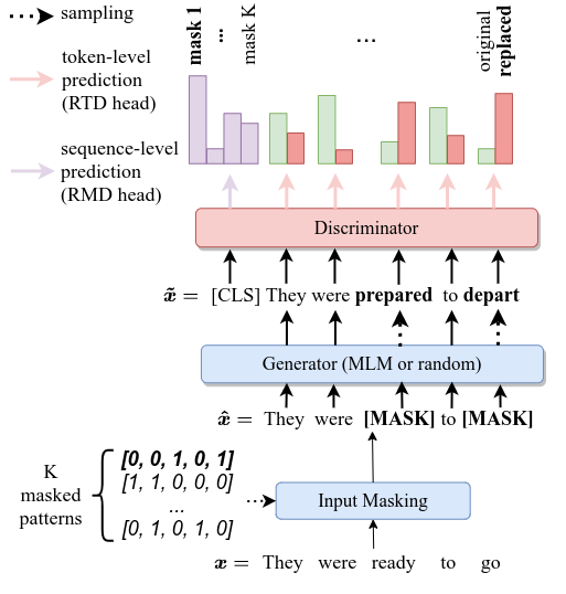
Figure 1: DATE Training. Firstly, the input sequence is masked using a sampled masked pattern and a generator fills in new tokens in place of the masked ones. Secondly, the discriminator receives supervision signals from two tasks: RMD (which mask pattern was applied to the input sequence) and RTD (the per-token status: original or replaced).

We notably simplify the computation of the Pseudo Label (PL) anomaly score Wang et al. (2019) by removing the dependency on running over multiple transformations and enabling it to work with token-level predictions. This significantly speeds up the PL score evaluation.

To our knowledge, DATE is the first end-to-end deep AD method on text that uses self-supervised classification models to produce normality scores. Our contributions are summarized below:

• We introduce a sequence-level self-supervised task called Replaced Mask Detection to distinguish between different transformations applied to a text. Jointly optimizing both sequence and token-level tasks stabilizes training, improving the AD performance.

• We compute an efficient Pseudo Label score for anomalies, by removing the need for evaluating multiple transformations, allowing it to work directly on individual tokens probabilities. This makes our model faster and its results more interpretable.

• We outperform existing state-of-the-art semi-supervised AD methods on text by a large margin (AUROC) on two datasets: 20Newsgroups (+13.5%) and AG News (+6.9%). Moreover, in unsupervised AD settings, even with 10% outliers in training data, DATE surpasses all other methods trained with 0% outliers.

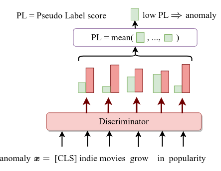
Figure 2: DATE Testing. The input text sequence is fed to the discriminator, resulting in token-level probabilities for the normal class, which are further aggregated into an anomaly score, as detailed in Sec.3.3. For deciding whether a sample is either normal or abnormal, we aggregate over all of its tokens.

2 Related Work

Our work relates to self-supervision for language representation as well as self-supervision for learning features of normality in AD.

2.1 Self-supervision for NLP

Self-supervision has been the bedrock of learning good feature representations in NLP. The earliest neural methods leveraged shallow models to produce static word embeddings such as word2vec Mikolov et al. (2013), GloVe Pennington et al. (2014) or fastText Bojanowski et al. (2017); Joulin et al. (2017). More recently, contextual word embeddings have produced state-of-the-art results in many NLP tasks, enabled by Transformer-based Vaswani et al. (2017) or LSTM-based Hochreiter and Schmidhuber (1997) architectures, trained with language modeling Peters et al. (2018); Radford et al. (2019) or masked language modeling Devlin et al. (2018) tasks.

Many improvements and adaptations have been proposed over the original BERT, which address other languages Martin et al. (2020); de Vries et al. (2019), domain specific solutions Beltagy et al. (2019); Lee et al. (2020) or more efficient pre-training models such as ALBERT Lan et al. (2019) or ELECTRA Clark et al. (2020). ELECTRA pre-trains a BERT-like generator and discriminator with a Replacement Token Detection (RTD) Task. The generator substitutes masked tokens with likely alternatives and the discriminator is trained to distinguish between the original and masked tokens.

2.2 Self-supervised classification for AD

Typical representation learning approaches to deep AD involve learning features of normality using autoencoders Hawkins et al. (2002); Sakurada and Yairi (2014); Chen et al. (2017) or generative adversarial networks Schlegl et al. (2017). More recent methods train the discriminator in a self-supervised fashion, leading to better normality features and anomaly scores. These solutions mostly focus on image data Golan and El-Yaniv (2018); Wang et al. (2019) and train a model to distinguish between different transformations applied to the images (e.g. rotation, flipping, shifting). An interesting property that justifies self-supervision under unsupervised AD is called inlier priority Wang et al. (2019), which states that during training, inliers (normal instances) induce higher gradient magnitudes than outliers, biasing the network’s update directions towards reducing their loss. Due to this property, the outputs for inliers are more consistent than for outliers, enabling them to be used as anomaly scores.

2.3 AD for text

There are a few shallow methods for AD on text, usually operating on traditional document-term matrices. One of them uses one-class SVMs Schölkopf et al. (2001a) over different sparse document representations Manevitz and Yousef (2001). Another method uses non-negative matrix factorization to decompose the term-document matrix into a low-rank and an outlier matrix Kannan et al. (2017). LDA-based Blei et al. (2003) clustering algorithms are augmented with semantic context derived from WordNet Miller (1995) or from the web to detect anomalies Mahapatra et al. (2012).

2.4 Deep AD for text

While many deep AD methods have been developed for other domains, few approaches use neural networks or pre-trained word embeddings for text anomalies. Earlier methods use autoencoders Manevitz and Yousef (2007) to build document representations. More recently, pre-trained word embeddings and self-attention were used to build contextual word embeddings Ruff et al. (2019). These are jointly optimized with a set of context vectors, which act as topic centroids. The network thus discovers relevant topics and transforms normal examples such that their contextual word embeddings stay close to the topic centroids. Under this setup, anomalous instances have contextual word embeddings which on average deviate more from the centroids.

3 Our Approach

Our method is called DATE for ’Detecting Anomalies in Text using ELECTRA’. We propose an end-to-end AD approach for the discrete text domain that combines our novel self-supervised task (Replaced Mask Detection), a powerful representation learner for text (ELECTRA), and an AD score tailored for sequential data. We present next the components of our model and a visual representation for the training and testing pipeline in Fig. 1-2.

3.1 Replaced Mask Detection task

We introduce a novel self-supervised task for text, called Replaced Mask Detection (RMD). This discriminative task creates training data by transforming an existing text using one out of K given operations. It further asks to predict the correct operation, given the transformed text. The transformation over the text consists of two steps: 1) masking some of the input words using a predefined mask pattern and 2) replacing the masked words with alternative ones (e.g. ’car’ with ’taxi’).

Input masking.

Let $\bm{m}\in\{0,1\}^{T}$ be a mask pattern corresponding to the text input $\bm{x}~{}=~{}[x_{1},x_{2},...,x_{T}]$. For training, we generate and fix $K$ mask patterns $\bm{m}^{(1)},\bm{m}^{(2)},...,\bm{m}^{(K)}$ by randomly sampling a constant number of ones. Instead of masking random tokens on-the-fly as in ELECTRA, we first sample a mask pattern from the K predefined ones. Next we apply it to the input, as in Fig. 1. Let $\bm{\hat{x}}(\bm{m})=[\hat{x}_{1},\hat{x}_{2},...,\hat{x}_{T}]$ be the input sequence $\bm{x}$, masked with $\bm{m}$, where:

$$\hat{x}_{i}=\begin{cases}x_{i},&\bm{m}_{i}=0\\ \texttt{[MASK]},&\bm{m}_{i}=1\end{cases}$$

For instance, given an input $\bm{x}=$ [bank, hikes, prices, before, election] and a mask pattern $\bm{m}=[0,0,1,0,1]$, the masked input is $\bm{\hat{x}}(\bm{m})=$ [bank, hikes, [MASK], before, [MASK]].

Replacing [MASK]s.

Each masked token can be replaced with a word token (e.g. by sampling uniformly from the vocabulary). For more plausible alternatives, masked tokens can be sampled from a Masked Language Model (MLM) generator such as BERT, which outputs a probability distribution $P_{G}$ over the vocabulary, for each token. Let $\widetilde{\bm{x}}(\bm{m})=[\widetilde{x}_{1},\widetilde{x}_{2},...,\widetilde{x}_{T}]$ be the plausibly corrupted text, where:

$$\widetilde{x_{i}}=\begin{cases}x_{i},&\bm{m}_{i}=0\\ w_{i}\sim P_{G}(x_{i}|\bm{\hat{x}}(\bm{m});\theta_{G}),&\bm{m}_{i}=1\end{cases}$$

For instance, given the masked input $\bm{\hat{x}}(\bm{m})=$ [bank, hikes, [MASK], before, [MASK]], a plausibly corrupted input is $\widetilde{\bm{x}}(\bm{m})=$ [bank, hikes, fees, before, referendum].

Connecting RMD and RTD tasks.

RTD is a binary sequence tagging task, where some tokens in the input are corrupted with plausible alternatives, similarly to RMD. The discriminator must then predict for each token if it’s the original token or a replaced one. Distinctly from RTD, which is a token-level discriminative task, RMD is a sequence-level one, where the model distinguishes between a fixed number of predefined transformations applied to the input. As such, RMD can be seen as the text counterpart task for the self-supervised classification of geometric alterations applied to images Golan and El-Yaniv (2018); Wang et al. (2019). While RTD predictions could be used to sequentially predict an entire mask pattern, they can lead to masks that are not part of the predefined K patterns. But the RMD constraint overcomes this behaviour. We thus train DATE to solve both tasks simultaneously, which increases the AD performance compared to solving one task only, as shown in Sec. 4.2. Furthermore, this approach also improves training stability.

3.2 DATE Architecture

We solve RMD and RTD by jointly training a generator, G, and a discriminator, D. G is an MLM used to replace the masked tokens with plausible alternatives. We also consider a setup with a random generator, in which we sample tokens uniformly from the vocabulary. D is a deep neural network with two prediction heads used to distinguish between corrupted and original tokens (RTD) and to predict which mask pattern was applied to the corrupted input (RMD). At test time, G is discarded and D’s probabilities are used to compute an anomaly score.

Both G and D models are based on a BERT encoder, which consists of several stacked Transformer blocks Vaswani et al. (2017). The BERT encoder transforms an input token sequence $\bm{x}~{}=~{}[x_{1},x_{2},...,x_{T}]$ into a sequence of contextualized word embeddings $h(\bm{x})=[h_{1},h_{2},...,h_{T}]$.

Generator.

G is a BERT encoder with a linear layer on top that outputs the probability distribution $P_{G}$ for each token. The generator is trained using the MLM loss:

$$\mathcal{L}_{MLM}=E\biggl{[}\sum_{\begin{subarray}{c}i=1;\\ s.t.m_{i}=1\end{subarray}}^{T}-\log P_{G}(x_{i}|\bm{\hat{x}}(\bm{m});\theta_{G})\biggr{]}$$ (1)

Discriminator.

D is a BERT encoder with two prediction heads applied over the contextualized word representations:

i. RMD head. This head outputs a vector of logits for all mask patterns $\bm{o}=[o_{1},...,o_{K}]$. We use the contextualized hidden vector $h_{\texttt{[CLS]}}$ (corresponding to the [CLS] special token at the beginning of the input) for computing the mask logits $\bm{o}$ and $P_{M}$, the probability of each mask pattern:

$$P_{M}(\bm{m}=\bm{m}^{(k)}|\widetilde{\bm{x}}(\bm{m}^{(k)});\theta_{D})=\frac{exp(o_{k})}{\sum_{i=1}^{K}exp(o_{i})}$$ (2)

ii. RTD head. This head outputs scores for the two classes (original and replaced) for each token $x_{1},x_{2},...,x_{T}$, by using the contextualized hidden vectors $h_{1},h_{2},...,h_{T}$.

Loss.

We train the DATE network in a maximum-likelihood fashion using the $\mathcal{L}_{DATE}$ loss:

$$\min_{\theta_{D},\theta_{G}}\sum_{\bm{x}\in\mathcal{X}}\mathcal{L}_{DATE}(\theta_{D},\theta_{G};\bm{x})$$ (3)

The loss contains both the token-level losses in ELECTRA, as well as the sequence-level mask detection loss $\mathcal{L}_{RMD}$:

$$\begin{split}\mathcal{L}_{DATE}(\theta_{D},\theta_{G};\bm{x})=\mu\mathcal{L}_{RMD}(\theta_{D};\bm{x})+\\ \mathcal{L}_{MLM}(\theta_{G};\bm{x})+\lambda\mathcal{L}_{RTD}(\theta_{D};\bm{x}),\end{split}$$ (4)

where the discriminator losses are:

$$\mathcal{L}_{RMD} =\mathop{\mathbb{E}}\biggl{[}-\log P_{M}(\bm{m}|\widetilde{\bm{x}}(\bm{m});\theta_{D})\biggr{]},$$ (5)

$$\mathcal{L}_{RTD} =\mathop{\mathbb{E}}\biggl{[}\sum_{\begin{subarray}{c}i=1;\\ x_{i}\neq\texttt{[CLS]}\end{subarray}}^{T}-\log P_{D}(m_{i}|\bm{\widetilde{\bm{x}}}(\bm{m});\theta_{D})\biggr{]},$$ (6)

where $P_{D}$ is the probability distribution that a token was replaced or not.

The ELECTRA loss enables D to learn good feature representations for language understanding. Our RMD loss puts the representation in a larger sequence-level context. After pre-training, G is discarded and D can be used as a general-purpose text encoder for downstream tasks. Output probabilities from D are further used to compute an anomaly score for new examples.

3.3 Anomaly Detection score

We adapt the Pseudo Label (PL) based score from the $E^{3}Outlier$ framework Wang et al. (2019) in a novel and efficient way. In its general form, the PL score aggregates responses corresponding to multiple transformations of $\bm{x}$. This approach requires $k$ input transformations over an input $\bm{x}$ and $k$ forward passes through a discriminator. It then takes the probability of the ground truth transformation and averages it over all $k$ transformations.

To compute PL for our RMD task, we take $\bm{x}$ to be our input text and the K mask patterns as the possible transformations. We corrupt $\bm{x}$ with mask $\bm{m}^{(i)}$ and feed the resulted text to the discriminator. We take the probability of the i-th mask from the RMD head. We repeat this process $k$ times and average over the probabilities of the correct mask pattern. This formulation requires $k$ feed-forward steps through the DATE network, which slows down inference. We propose a more computationally efficient approach next.

PL over RTD classification scores.

Instead of aggregating sequence-level responses from multiple transformations over the input, we can aggregate token-level responses from a single model over the input to compute an anomaly score. More specifically, we can discard the generator and feed the original input text to the discriminator directly. We then use the probability of each token being original (not corrupted) and then average over all the tokens in the sequence:

$$PL_{RTD}(x)=\frac{1}{T}\sum_{i=1}^{T}P_{D}(m_{i}=0|\bm{\widetilde{\bm{x}}}(\bm{m}^{(0)});\theta_{D}),$$ (7)

where $\bm{m}^{(0)}=[0,0,...,0]$ effectively leaves the input unchanged. As can be seen in Fig. 2, the RTD head will be less certain in predicting the original class for outliers (having a probability distribution unseen at training time), which will lead to lower PL scores for outliers and higher PL scores for inliers. We use PL at testing time, when the entire input is either normal or abnormal. Our method also speeds up inference, since we only do one feed-forward pass through the discriminator instead of $k$ passes. Moreover, having a per token anomaly score helps us better understand and visualize the behavior of our model, as shown in Fig. 4.

4 Experimental analysis

In this section, we detail the empirical validation of our method by presenting: the semi-supervised and unsupervised experimental setup, a comprehensive ablation study on DATE, and the comparison with state-of-the-art on the semi-supervised and unsupervised AD tasks. DATE does not use any form of pre-training or knowledge transfer (from other datasets or tasks), learning all the embeddings from scratch. Using pre-training would introduce unwanted prior knowledge about the outliers, making our model considering them known (normal).

4.1 Experimental setup

We describe next the Anomaly Detection setup, the datasets and the implementation details of our model. We make the code publicly available .

Anomaly Detection setup.

We use a semi-supervised setting in Sec. 4.2-4.3 and an unsupervised one in Sec. 4.4. In the semi-supervised case, we successively treat one class as normal (inliers) and all the other classes as abnormal (outliers). In the unsupervised AD setting, we add a fraction of outliers to the inliers training set, thus contaminating it. We compute the Area Under the Receiver Operating Curve (AUROC) for comparing our method with the previous state-of-the-art. For a better understanding of our model’s performance in an unbalanced dataset, we report the Area Under the Precision-Recall curve (AUPR) for inliers and outliers per split in the supplementary material C.

Datasets.

We test our solution using two text classification datasets, after stripping headers and other metadata. For the first dataset, 20Newsgroups, we keep the exact setup, splits, and preprocessing (lowercase, removal of: punctuation, number, stop word and short words) as in Ruff et al. (2019), ensuring a fair comparison with previous text anomaly detection methods. As for the second dataset, we use a significantly larger one, AG News, better suited for deep learning methods. 1) 20Newsgroups : We only take the articles from six top-level classes: computer, recreation, science, miscellaneous, politics, religion, like in Ruff et al. (2019). This dataset is relatively small, but a classic for NLP tasks (for each class, there are between 577-2856 samples for training and 382-1909 for validation). 2) AG News Zhang et al. (2015): This topic classification corpus was gathered from multiple news sources, for over more than one year . It contains four topics, each class with 30000 samples for training and 1900 for validation.

Model and Training.

For training the DATE network we follow the pipeline in Fig. 1. In addition to the parameterized generator, we also consider a random generator, in which we replace the masked tokens with samples from a uniform distribution over the vocabulary. The discriminator is composed of four Transformer layers, with two prediction heads on top (for RMD and RTD tasks). We provide more details about the model in the supplementary material B. We train the networks with AdamW with amsgrad Loshchilov and Hutter (2019), $1e^{-5}$ learning rate, using sequences of maximum length $128$ for AG News, and $498$ for 20Newsgroups. We use $K=50$ predefined masks, covering $50\%$ of the input for AG News and $K=25$, covering $25\%$ for 20Newsgroups. The training converges on average after $5000$ update steps and the inference time is $0.005$ sec/sample in PyTorch Paszke et al. (2017), on a single GTX Titan X.

4.2 Ablation studies

To better understand the impact of different components in our model and making the best decisions towards a higher performance, we perform an extensive set of experiments (see Tab. 1). Note that we successively treat each AG News split as inlier and report the mean and standard deviations over the four splits. The results show that our model is robust to domain shifts.

Abl.	Method	Variation	AUROC(%)
	CVDD	best	83.1 $\pm$ 4.4
	OCSVM	best	84.0 $\pm$ 5.0
	ELECTRA	adapted for AD	84.6 $\pm$ 4.5
	DATE	(Ours)	90.0 $\pm$ 4.2
A.	Anomaly score	MP	72.4 $\pm$ 3.7
		NE	73.1 $\pm$ 3.9
B.	Generator	small	89.3 $\pm$ 4.2
		large	89.8 $\pm$ 4.4
C.	Loss func	RTD only	89.4 $\pm$ 4.4
		RMD only	85.9 $\pm$ 4.1
D.	Masking	5 masks	87.5 $\pm$ 4.5
	patterns	10 masks	89.2 $\pm$ 4.3
		25 masks	89.8 $\pm$ 4.3
		100 masks	89.8 $\pm$ 4.3
E.	Mask percent	15%	89.5 $\pm$ 4.1
		25%	89.5 $\pm$ 4.1

Table 1: Ablation study. We show results for the competition and report ablation experiments which are only one change away from our best DATE configuration: A. $PL_{RTD}$; B. Rand C. RTD + RMD; D. 50 masks; E. 50%. For the ELECTRA line, we use: A. $PL_{RTD}$; B. Rand; C. RTD only; D. Unlimited; E. 15%. A. The Anomaly Score used over classification probabilities shows that $PL_{RTD}$ (used in DATE) is the best in predicting anomalies, meaning that our self-supervised classification task is well defined, with few ambiguous samples; B. A learned Generator does not justify its training cost; C. RMD Loss proved to be complementary with RTD Loss, their combination (in DATE) increasing the score and stabilizes the training; D+E.

A. Anomaly score. We explore three anomaly scores introduced in the $E^{3}Outlier$ framework Wang et al. (2019) on semi-supervised and unsupervised AD tasks in Computer Vision: Maximum Probability (MP), Negative Entropy (NE) and our modified Pseudo Label ($PL_{RTD}$). These scores are computed using the softmax probabilities from the final classification layer of the discriminator. PL is an ideal score if the self-supervised task manages to build and learn well separated classes. The way we formulate our mask prediction task enables a very good class separation, as theoretically proved in detail in the supplementary material A. Therefore, $PL_{RTD}$ proves to be significantly better in detecting the anomalies compared with MP and NE metrics, which try to compensate for ambiguous samples.

B. Generator performance. We tested the importance of having a learned generator, by using a one-layer Transformer with hidden size 16 (small) or 64 (large). The random generator proved to be better than both parameterized generators.

C. Loss function. For the final loss, we combined RTD (which sanctions the prediction per token) with our RMD (which enforces the detection of the mask applied on the entire sequence). We also train our model with RTD or RMD only, obtaining weaker results. This proves that combining losses with supervisions at different scales (locally: token-level and globally: sequence-level) improves AD performance. Moreover, when using only the RTD loss, the training can be very unstable (AUROC score peaks in the early stages, followed by a steep decrease). With the combined loss, the AUROC is only stationary or increases with time.

D. Masking patterns. The mask patterns are the root of our task formulation, hiding a part of the input tokens and asking the discriminator to classify them. As experimentally shown, having more mask patterns is better, encouraging increased expressiveness in the embeddings. Too many masks on the other hand can make the task too difficult for the discriminator and our ablation shows that having more masks does not add any benefit after a point. We validate the percentage of masked tokens in E. Mask percent ablation.

4.3 Comparison with other AD methods

We compare our method against classical AD baselines like Isolation Forest Liu et al. (2008) and existing state-of-the-art OneClassSVMs Schölkopf et al. (2001b) and CVDD Ruff et al. (2019). We outperform all previously reported performances on all 20Newsgroups splits by a large margin: 13.5% over the best reported CVDD and 11.7% over the best OCSVM, as shown in Tab. 4.3. In contrast, DATE uses the same set of hyper-parameters for a dataset, for all splits. For a proper comparison, we keep the same experimental setup as the one introduced in Ruff et al. (2019).

	Inlier
	IsoForest
	OCSVM
	CVDD
	DATE (Ours)
20 News	comp	66.1	78.0	74.0	92.1
	rec	59.4	70.0	60.6	83.4
	sci	57.8	64.2	58.2	69.7
	misc	62.4	62.1	75.7	86.0
	pol	65.3	76.1	71.5	81.9
	rel	71.4	78.9	78.1	86.1
AG News	business	79.6	79.9	84.0	90.0
	sci	76.9	80.7	79.0	84.0
	sports	84.7	92.4	89.9	95.9
	world	73.2	83.2	79.6	90.1

Table 2: Semi-supervised performance (AUROC%). We test on the 20Newsgroups and AG News datasets, by comparing DATE against several strong baselines and state-of-the-art solutions (with multiple variations, choosing the best score per split as detailed in Sec. 4.3): IsoForest, OCSVM, and CVDD. We largely outperform competitors with an average improvement of 13.5% on 20Newsgroups and 6.9% on AG News compared with the next best solution. Note that DATE uses the same set of hyper-parameters per dataset.

Isolation Forest.

We apply it over fastText or Glove embeddings, varying the number of estimators $(64,100,128,256)$, and choosing the best model per split. In the unsupervised AD setup, we manually set the percent of outliers in the train set.

OCSVM.

We use the One-Class SVM model implemented in the CVDD work . For each split, we choose the best configuration (fastText vs Glove, rbf vs linear kernel, $\nu$ $\in$ [0.05, 0.1, 0.2, 0.5]).

CVDD.

This model Ruff et al. (2019) is the current state-of-the-art solution for AD on text. For each split, we chose the best column out of all reported context sizes ($r$). The scores reported using the $c^{*}$ context vector depends on the ground truth and it only reveals "the potential of contextual anomaly detection", as the authors mention.

4.4 Unsupervised AD

We further analyse how our algorithm works in a fully unsupervised scenario, namely when the training set contains some anomalous samples (which we treat as normal ones). By definition, the quantity of anomalous events in the training set is significantly lower than the normal ones. In this experiment, we show how our algorithm performance is influenced by the percentage of anomalies in training data. Our method proves to be extremely robust, surpassing state-of-the-art, which is a semi-supervised solution, trained over a clean dataset (with 0% anomalies), even at 10% contamination, with +0.9% in AUROC (see Fig. 3). By achieving an outstanding performance in the unsupervised setting, we make unsupervised AD in text competitive against other semi-supervised methods. The reported scores are the mean over all AG News splits. We compare against the same methods presented in Sec. 4.3.

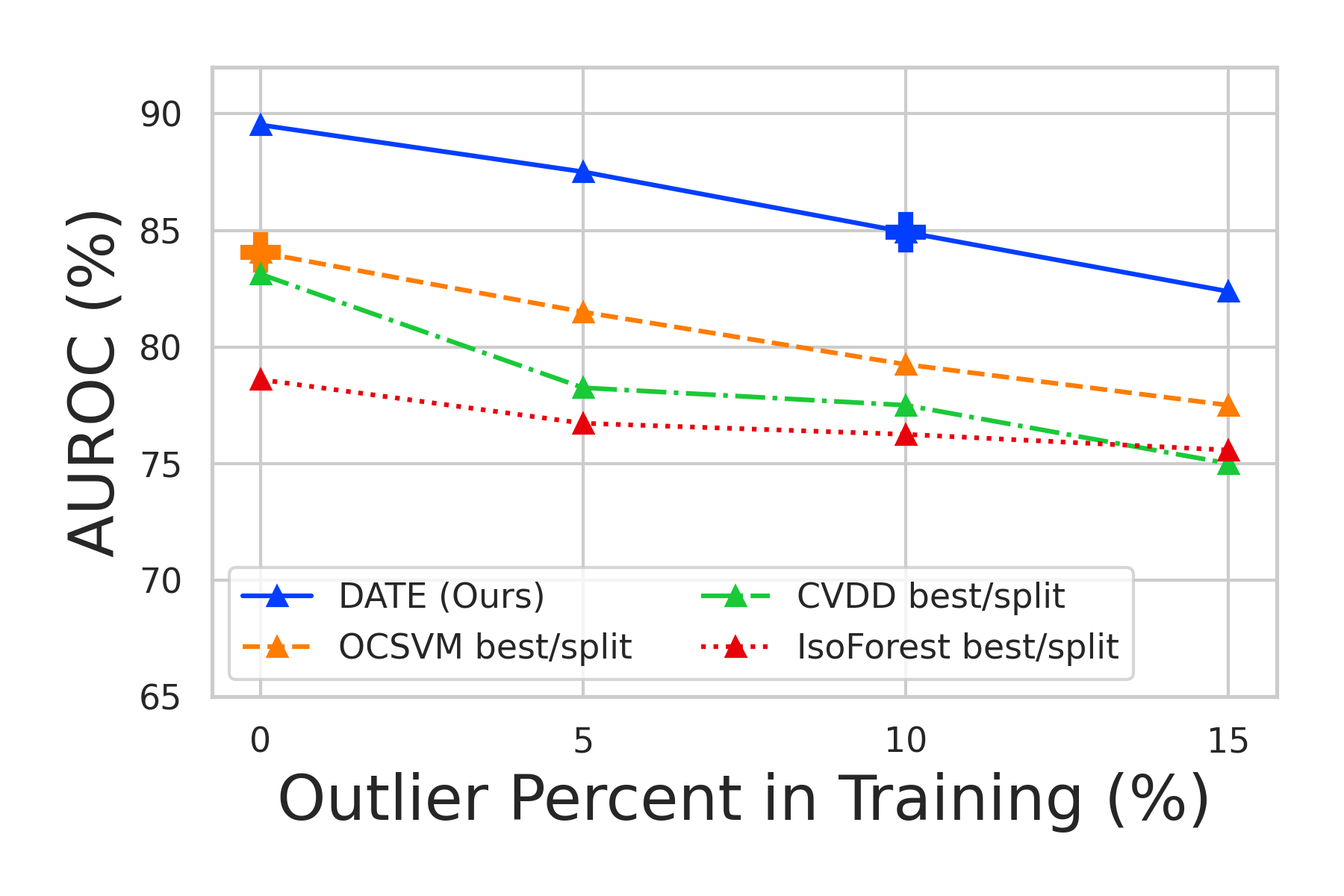
Figure 3: Unsupervised AD. We test the performance of our method when training on impure data, which contains anomalies in various percentages: 0%-15%. The performance slowly decreases when we increase the anomaly percentage, but even at 10% contamination, it is still better than state-of-the-art results on self-supervised anomaly detection in text Ruff et al. (2019), which trains on 0% anomalous data, proving the robustness of our method. Experiments were done on all AG News splits.

4.5 Qualitative results

We show in Fig. 4 how DATE performs in identifying anomalies in several examples. Each token is colored based on its PL score.

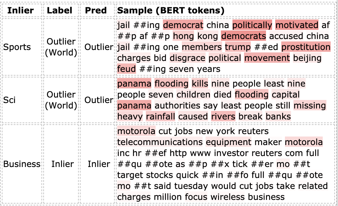
Figure 4: Qualitative examples. Lower scores are shown in a more intense red, and point to anomalies. In the $1^{st}$ example, words from politics are flagged as anomalous for sports. In the $2^{nd}$ one, words describing natural events are outliers for technology. In the $3^{rd}$ row, while few words have higher anomaly potential for the business domain, most of them are appropriate.

Figure 5: Normalized histogram for anomaly score. We see how the anomaly score (PL) distribution varies among inliers and outliers, from the beginning of the training ($1^{st}$ column) to the end ($2^{nd}$ column), where the two become well separated, with relatively low interference between classes. Note that a better separation is correlated with high performance ($1^{st}$ line split has $95.9\%$ AUROC, while the $2^{nd}$ has only $90.1\%$).

Separating anomalies.

We show how our anomaly score (PL) is distributed among normal vs abnormal samples. For visualization, we chose two splits from AG News and report the scores from the beginning of the training to the end. We see in Fig. 5 that, even though at the beginning, the outliers’ distribution of scores fully overlaps with the inliers, at the end of training the two are well separated, proving the effectiveness of our method.

5 Conclusion

We propose DATE, a model for tackling Anomaly Detection in Text, and formulate an innovative self-supervised task, based on masking parts of the initial input and predicting which mask pattern was used. After masking, a generator reconstructs the initially masked tokens and the discriminator predicts which mask was used. We optimize a loss composed of both token and sequence-level parts, taking advantage of powerful supervision, coming from two independent pathways, which stabilizes learning and improves AD performance. For computing the anomaly score, we alleviate the burden of aggregating predictions from multiple transformations by introducing an efficient variant of the Pseudo Label score, which is applied per token, only on the original input. We show that this score separates very well the abnormal entries from normal ones, leading DATE to outperform state-of-the-art results on all AD splits from 20Newsgroups and AG News datasets, by a large margin, both in the semi-supervised and unsupervised AD settings.

Acknowledgments.

This work has been supported in part by UEFISCDI, under Project PN-III-P2-2.1-PTE-2019-0532.

Appendix A Disjoint patterns analysis

We start from two observations regarding the performance of DATE, our Anomaly Detection algorithm. First, a discriminative task performs better if the classes are well separated Deng (2012) and there is a low probability for confusions. Second, the PL score for anomalies achieves best performance when the probability distribution for its input is clearly separated. Intuitively, for three classes, PL([0.9, 0.05, 0.05]) is better than PL([0.5, 0.3, 0.2]) because it allows PL to give either near $1$ score if the class is correct, either near $0$ score if it is not, avoiding the zone in the middle where we depend on a well chosen threshold.

Since the separation between the mask patterns greatly influences our final performance, we next analyze our AD task from the mask pattern generation point of view. Ideally, we want to have a sense of how disjoint our randomly sampled patterns are and make an informed choice for the pattern generation hyper-parameters.

First, we start by computing an upper bound for the probability of having two patterns with at least $p$ common masked points. We have $\binom{S}{M}$ patterns, where $S$ is the sequence length and $M$ is the number of masked tokens. We fix the first $p$ positions that we want to mask in any pattern. Considering those fixed masks, the probability of having a sequence with $M$ masked tokens, with $p$ tokens in the first positions is $r$:

$$r=\frac{\binom{S-p}{M-p}}{\binom{S}{M}}.$$ (8)

Next, the probability that two sequences mask the first $p$ tokens is $r^{2}$. But we can choose those two positions in a $\binom{S}{p}$ ways. So the probability that any two sequences have at least $p$ common masked tokens is lower than $UB_{2}$:

$$UB_{2}=\binom{S}{p}r$$ (9)

Next, out of our generated patterns, we sample $N$ masks, so the probability becomes less than the upper bound $UB_{N}$:

$$UB_{N} =\binom{N}{2}UB_{2}=\binom{N}{2}\binom{S}{p}r^{2}$$ (10)

$$=\binom{N}{2}\binom{S}{p}(\frac{\binom{S-p}{M-p}}{\binom{S}{M}})^{2}.$$

In our experiments, the sequence length is $S=128$ and we chose the number of masked tokens to be between 15% and 50% ($M$ between 19 and 64). We consider that two patterns are disjoint when they have less than $p$ masked tokens in common, for $N$ sampled patterns.

The probability that any two patterns collide (have more than $p$ masked tokens in common) is very low. We compute several values for its upper bound: $UB_{N=100,p=12}=5e-4$, $UB_{N=100,p=15}=1e-9$, $UB_{N=10,p=15}=1e-11$, $UB_{N=10,p=13}=1e-7$.

In conclusion, for our specific setup, the probability for two masks to largely overlap (large $p$ compared with $S$) is extremely small, ensuring us a good performance in the discriminator. We take advantage of this property of our pretext task by combining the discriminator output probabilities with the PL score.

Appendix B Model implementation

We add next more details on the implementation of the modules: from the ablation experiments in Tab. 1, Generator (small): 1 Transformer layer, with 4 self-attention heads, token and positional embeddings of size 128, hidden layer of size 16, feedforward layer of sizes 1024 and 16; Generator (large): 1 Transformer layer, with 4 self-attention heads, token and positional embeddings of size 128, hidden layer of size 64, feedforward layer of sizes 1024 and 64; As empirical experiments showed us, we choose a random Generator (samples were drawn from a uniform distribution over the vocabulary) in our final model. Discriminator: 4 Transformer layers, each with 4 self-attention heads, hidden layers of size 256, feedforward layers of sizes of 1024 and 256, 128-dimensional token and positional embeddings, which are tied with the generator. For other unspecified hyper-parameters we use the ones in ELECTRA-Small model. Prediction Heads: both heads have 2 linear layers separated by a non-linearity, ending in a classification. Loss weights: We set the RTD $\lambda$ weight to 50 as in Clark et al. (2020), and the RMD $\mu$ weight to 100.

Appendix C More qualitative and quantitative Results

In Fig. 6 we show more qualitative results, trained on different inliers. To encourage further more detailed comparisons, we report the AUPR metric on AG News for inliers and outliers (see Tab. 3). When all the other metrics are almost saturated, we notice that AUPR-in better captures the performance on a certain split.

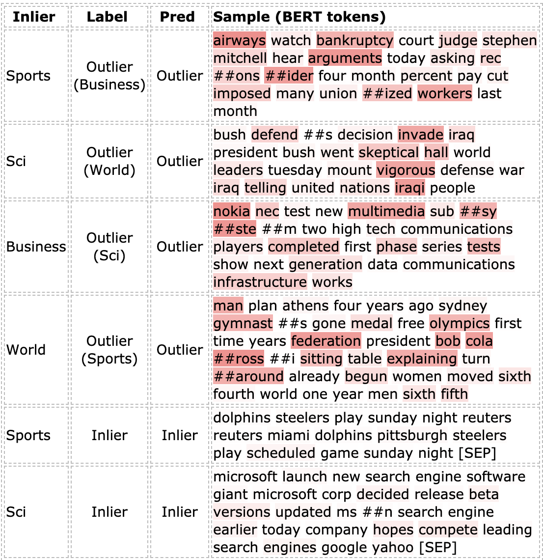
Figure 6: More qualitative examples.

Subset	business	sci	sports	world
AUPR-in	74.8	62.4	88.8	81.9
AUPR-out	96.1	93.5	98.5	95.5

Table 3: We report AUPR metric for AG News splits, on inliers and outliers since this is a more relevant metric for unbalanced classes (which is the case for all splits in text AD, as explained in Anomalies setup).

References

- Aggarwal (2015) Charu C Aggarwal. 2015. Outlier analysis. In Data mining, pages 237–263. Springer.
- Banoth et al. (2017) Lalu Banoth, Mnr Teja, M Saicharan, and Naveen Chandra. 2017. A survey of data mining and machine learning methods for cyber security intrusion detection. International Journal of Research, 4:406–412.
- Beltagy et al. (2019) Iz Beltagy, Kyle Lo, and Arman Cohan. 2019. Scibert: A pretrained language model for scientific text. In EMNLP/IJCNLP.
- Blei et al. (2003) David M. Blei, Andrew Y. Ng, and Michael I. Jordan. 2003. Latent dirichlet allocation. J. Mach. Learn. Res., 3(null):993–1022.
- Bojanowski et al. (2017) Piotr Bojanowski, Edouard Grave, Armand Joulin, and Tomas Mikolov. 2017. Enriching word vectors with subword information. Transactions of the Association for Computational Linguistics, 5:135–146.
- Chandola et al. (2009) Varun Chandola, Arindam Banerjee, and Vipin Kumar. 2009. Anomaly detection: A survey. ACM computing surveys (CSUR), 41(3):1–58.
- Chen et al. (2017) Jinghui Chen, Saket Sathe, Charu C. Aggarwal, and Deepak S. Turaga. 2017. Outlier detection with autoencoder ensembles. In SDM.
- Clark et al. (2020) Kevin Clark, Minh-Thang Luong, Quoc V. Le, and Christopher D. Manning. 2020. Electra: Pre-training text encoders as discriminators rather than generators. ArXiv, abs/2003.10555.
- de Vries et al. (2019) Wietse de Vries, Andreas van Cranenburgh, Arianna Bisazza, Tommaso Caselli, Gertjan van Noord, and Malvina Nissim. 2019. Bertje: A dutch bert model. ArXiv, abs/1912.09582.
- Deng (2012) L. Deng. 2012. The mnist database of handwritten digit images for machine learning research [best of the web]. IEEE Signal Processing Magazine, 29:141–142.
- Devlin et al. (2018) Jacob Devlin, Ming-Wei Chang, Kenton Lee, and Kristina Toutanova. 2018. BERT: pre-training of deep bidirectional transformers for language understanding. CoRR, abs/1810.04805.
- Dorronsoro et al. (1997) J. Dorronsoro, Francisco Ginel, C. Sanchez, and C. Cruz. 1997. Neural fraud detection in credit card operations. IEEE transactions on neural networks, 84:827–34.
- Golan and El-Yaniv (2018) Izhak Golan and Ran El-Yaniv. 2018. Deep anomaly detection using geometric transformations. CoRR, abs/1805.10917.
- Hawkins (1980) Douglas M Hawkins. 1980. Identification of outliers, volume 11. Springer.
- Hawkins et al. (2002) Simon Hawkins, Hongxing He, Graham J. Williams, and Rohan A. Baxter. 2002. Outlier detection using replicator neural networks. In Proceedings of the 4th International Conference on Data Warehousing and Knowledge Discovery, DaWaK 2000, page 170–180, Berlin, Heidelberg. Springer-Verlag.
- Hochreiter and Schmidhuber (1997) Sepp Hochreiter and Jürgen Schmidhuber. 1997. Long short-term memory. Neural Comput., 9(8):1735–1780.
- Joulin et al. (2017) Armand Joulin, Edouard Grave, Piotr Bojanowski, and Tomas Mikolov. 2017. Bag of tricks for efficient text classification. Proceedings of the 15th Conference of the European Chapter of the Association for Computational Linguistics: Volume 2, Short Papers.
- Kammerer et al. (2019) Klaus Kammerer, Burkhard Hoppenstedt, Rüdiger Pryss, Steffen Stökler, Johannes Allgaier, and M. Reichert. 2019. Anomaly detections for manufacturing systems based on sensor data—insights into two challenging real-world production settings. Sensors (Basel, Switzerland), 19.
- Kannan et al. (2017) Ramakrishnan Kannan, Hyenkyun Woo, Charu C. Aggarwal, and Haesun Park. 2017. Outlier detection for text data : An extended version. CoRR, abs/1701.01325.
- Lan et al. (2019) Zhenzhong Lan, Mingda Chen, Sebastian Goodman, Kevin Gimpel, Piyush Sharma, and Radu Soricut. 2019. Albert: A lite bert for self-supervised learning of language representations.
- Lee et al. (2020) Jinhyuk Lee, Wonjin Yoon, Sungdong Kim, D. Kim, Sunkyu Kim, Chan Ho So, and Jaewoo Kang. 2020. Biobert: a pre-trained biomedical language representation model for biomedical text mining. Bioinformatics.
- Liu et al. (2008) Fei Tony Liu, Kai Ming Ting, and Zhi-Hua Zhou. 2008. Isolation forest. In 2008 Eighth IEEE International Conference on Data Mining, pages 413–422. IEEE.
- Loshchilov and Hutter (2019) Ilya Loshchilov and Frank Hutter. 2019. Decoupled weight decay regularization. In ICLR 2019.
- Mahapatra et al. (2012) Amogh Mahapatra, Nisheeth Srivastava, and Jaideep Srivastava. 2012. Contextual anomaly detection in text data. Algorithms, 5(4):469–489.
- Manevitz and Yousef (2001) L. Manevitz and M. Yousef. 2001. One-class svms for document classification. J. Mach. Learn. Res., 2:139–154.
- Manevitz and Yousef (2007) L. Manevitz and M. Yousef. 2007. One-class document classification via neural networks. Neurocomputing, 70:1466–1481.
- Martin et al. (2020) Louis Martin, Benjamin Muller, Pedro Javier Ortiz Suárez, Yoann Dupont, Laurent Romary, ’Eric de la Clergerie, Djamé Seddah, and Benoît Sagot. 2020. Camembert: a tasty french language model. ArXiv, abs/1911.03894.
- Mikolov et al. (2013) Tomas Mikolov, Kai Chen, Gregory S. Corrado, and Jeffrey Dean. 2013. Efficient estimation of word representations in vector space. CoRR, abs/1301.3781.
- Miller (1995) George A. Miller. 1995. Wordnet: A lexical database for english. Commun. ACM, 38(11):39–41.
- Paszke et al. (2017) Adam Paszke, Sam Gross, Soumith Chintala, Gregory Chanan, Edward Yang, Zachary DeVito, Zeming Lin, Alban Desmaison, Luca Antiga, and Adam Lerer. 2017. Automatic differentiation in pytorch.
- Pennington et al. (2014) Jeffrey Pennington, Richard Socher, and Christopher D. Manning. 2014. Glove: Global vectors for word representation. In Empirical Methods in Natural Language Processing (EMNLP), pages 1532–1543.
- Peters et al. (2018) Matthew Peters, Mark Neumann, Mohit Iyyer, Matt Gardner, Christopher Clark, Kenton Lee, and Luke Zettlemoyer. 2018. Deep contextualized word representations. Proceedings of the 2018 Conference of the North American Chapter of the Association for Computational Linguistics: Human Language Technologies, Volume 1 (Long Papers).
- Radford et al. (2019) A. Radford, Jeffrey Wu, R. Child, David Luan, Dario Amodei, and Ilya Sutskever. 2019. Language models are unsupervised multitask learners.
- Ruff et al. (2019) Lukas Ruff, Yury Zemlyanskiy, Robert Vandermeulen, Thomas Schnake, and Marius Kloft. 2019. Self-attentive, multi-context one-class classification for unsupervised anomaly detection on text. In Proceedings of the 57th Annual Meeting of the Association for Computational Linguistics, pages 4061–4071, Florence, Italy. Association for Computational Linguistics.
- Sakurada and Yairi (2014) Mayu Sakurada and Takehisa Yairi. 2014. Anomaly detection using autoencoders with nonlinear dimensionality reduction. In Proceedings of the MLSDA 2014 2nd Workshop on Machine Learning for Sensory Data Analysis, MLSDA’14, page 4–11, New York, NY, USA. Association for Computing Machinery.
- Schlegl et al. (2017) Thomas Schlegl, Philipp Seeböck, Sebastian M. Waldstein, Ursula Schmidt-Erfurth, and Georg Langs. 2017. Unsupervised anomaly detection with generative adversarial networks to guide marker discovery. In IPMI.
- Schölkopf et al. (2001a) B. Schölkopf, John C. Platt, J. Shawe-Taylor, A. Smola, and R. Williamson. 2001a. Estimating the support of a high-dimensional distribution. Neural Computation, 13:1443–1471.
- Schölkopf et al. (2001b) Bernhard Schölkopf, John C Platt, John Shawe-Taylor, Alex J Smola, and Robert C Williamson. 2001b. Estimating the support of a high-dimensional distribution. Neural computation, 13(7):1443–1471.
- Vaswani et al. (2017) Ashish Vaswani, Noam Shazeer, Niki Parmar, Jakob Uszkoreit, Llion Jones, Aidan N. Gomez, Lukasz Kaiser, and Illia Polosukhin. 2017. Attention is all you need. CoRR, abs/1706.03762.
- Wang et al. (2019) S. Wang, Y. Zeng, Xinwang Liu, En Zhu, Jianping Yin, Chuanfu Xu, and M. Kloft. 2019. Effective end-to-end unsupervised outlier detection via inlier priority of discriminative network. In NeurIPS.
- Zhang et al. (2015) Xiang Zhang, Junbo Jake Zhao, and Yann LeCun. 2015. Character-level convolutional networks for text classification. In NeurIPS.