3D convection-resolving model of temperate, tidally-locked exoplanets

Abstract

A large fraction of known terrestrial-size exoplanets located in the Habitable Zone of M-dwarfs are expected to be tidally-locked. Numerous efforts have been conducted to study the climate of such planets, using in particular 3-D Global Climate Models (GCM). One of the biggest challenges in simulating such an extreme environment is to properly represent the effects of sub-grid convection. Most GCMs use either a simplistic convective-adjustment parametrization or sophisticated (e.g., mass flux scheme) Earth-tuned parametrizations. One way to improve the representation of convection is to study convection using Convection Resolving numerical Models (CRMs), with an fine spatial resolution . In this study, we developed a CRM coupling the non-hydrostatic dynamical core WRF with the radiative transfer and cloud/precipitation models of the LMD-Generic climate model to study convection and clouds on tidally-locked planets, with a focus on Proxima b. Simulations were performed for a set of 3 surface temperatures (corresponding to three different incident fluxes) and 2 rotation rates, assuming an Earth-like atmosphere. The main result of our study is that while we recover the prediction of GCMs that (low-altitude) cloud albedo increases with increasing stellar flux, the cloud feedback is much weaker due to transient aggregation of convection leading to low partial cloud cover.

1 Introduction

The habitable zone (HZ) is classically defined as the range of orbital distances for which a planet can sustain water in liquid phase at the surface Kasting et al., (1993), providing a potentially suitable environment (surface, liquid water, photons) for the emergence of life as we know it on Earth. Depending on the rotation state and the atmospheric composition of the planet, various processes can either extend or narrow the HZ. While the presence of greenhouse gases tends to increase the surface temperature, the radiative effect of clouds can be much more subtle. Clouds can scatter (and thus reflect) as well as absorb a significant part of incident stellar radiation. But they can also absorb (and scatter) the infrared thermal emission from the surface and the atmosphere, and then re-emit (or back-scatter, respectively) infrared thermal radiation back to the surface.

On Earth, the relative ratio between cloud-free and cloudy area in the tropics have a strong effect on the mean temperature (Pierrehumbert,, 1995). It is therefore crucial to know the composition, thickness, vertical and horizontal spatial distributions of these clouds to correctly evaluate the climate state of the Earth and by extension of other planets in or outside of the solar system.

Most terrestrial-sized exoplanets located in the HZ that have been detected so far (Anglada-Escudé et al.,, 2016; Gillon et al.,, 2017; Bonfils et al.,, 2018; Zechmeister et al.,, 2019; Tuomi et al.,, 2019) are orbiting around low mass stars, also known as M-stars, the most abundant and longest-lived stars in the Milky Way (Kirkpatrick et al.,, 2012). A significant number of the planets orbiting in the Habitable Zone of low mass stars are expected to have near-zero obliquity and be in synchronous rotation around their host star (i.e. with one side of the planet permanently facing its host star). On a synchronously rotating telluric exoplanet covered with water, the constant stellar radiation received at the substellar point should create a strong convective region producing very thick clouds reflecting the stellar light (Yang et al.,, 2013). This behaviour has been shown to be robust across a wide range of 3-dimensional Global Climate Models (Yang et al., 2019b, ). The more irradiation a synchronous planet receives, the stronger the moist convection and thus the more reflective the substellar cloud cover is (Yang et al.,, 2013). As a result, the inner edge of the HZ for synchronously rotating planets was found to lie significantly closer to the host star (Yang et al.,, 2013). This mechanism may be less effective for synchronous planets in the fast-rotating regime, i.e. with orbital periods roughly lower than 10 days (Edson et al.,, 2011; Haqq-Misra et al.,, 2018). For these planets, winds are strong enough to shift the clouds away from the substellar point (Kopparapu et al.,, 2016), thus reducing the effective cloud coverage in the substellar region, where the peak of instellation is. This effect weakens the cloud feedback described above (Kopparapu et al.,, 2016). This effect highlights the importance of knowing accurately the composition, thickness, as well as the vertical and horizontal distributions of clouds on a synchronously rotating planet to get insight on its mean climate state.

The representation of clouds and turbulence in the Global Climate Models (GCMs) is one of the most important uncertainties of these models. In fact, the typical size of the structures of these phenomena, i.e. the shallow convection cells diameter, varies on Earth from 10 to 40 km (Atkinson and Wu Zhang,, 1996). This is much lower than the typical horizontal resolution of GCMs ($\sim$ 100 km). GCMs use therefore sub-grid parameterizations to represent the effects of convection and turbulence, which is a main source of uncertainty in the models (Yang et al., 2019b, ; Fauchez et al.,, 2019). In fact, these schemes are either (i) too simple to represent the mixing of wind, energy and tracer by the convection, or either (ii) sophisticated, but tuned to simulate present-day Earth, and can therefore give inaccurate results when used to simulate environments very different from the Earth, such as planets in synchronous rotation. To be able to resolve convection in such exotic environments (in order to better understand them), it is necessary to run models at a spatial resolution similar to that at which convection processes operate.

Correctly modeling convection on synchronously rotating planets is not only crucial to their mean climate state and thus their potential habitability, but is also key to the observability of these planets in reflected light. Direct imaging in reflected light is indeed one of the most promising avenue to detect and characterize temperate, Earth-size planets orbiting around nearby stars. Specifically, it has been shown that the reflected light of very nearby temperate planets such as Proxima b (Anglada-Escudé et al.,, 2016) could be detected and analysed with ELT-class telescopes (Turbet et al.,, 2016). Lovis et al., (2017) even proposed that, combining direct imaging with high-resolution spectroscopy on a 8 m-class telescope, observations of Proxima b, in particular in reflected light could be attempted. However, our ability to detect and characterize Proxima b (and its atmosphere, surface, and clouds) depends strongly on the amount of light reflected by the planet. This amount highly depends on the reflectivity of the cloud cover (especially near and eastward of the substellar region), where the signal measured by direct imaging is more favorable.

On Earth intense convective activity occurs in the tropics leading to a cloud coverage of about 70$\%$ above the oceans (Eastman et al.,, 2011; Stubenrauch et al.,, 2006). Several types of clouds play a distinct role in that net coverage. In the tropics the low altitude stratocumulus covers 20 $\%$ of the surface, mesoscale high opaque clouds 6 $\%$ and cirrus clouds about 45 $\%$. Since the 80’s, some models were developed with the aim to study the convection (Lipps and Hemler,, 1986, 1988) and its organization (Held et al.,, 1993). With evolution of computing capacity, the model evolved from two-dimensional models (Grabowski,, 2001; Grabowski and Moncrieff,, 2002), to three-dimensional channels configuration models (Tompkins,, 2001; Wing and Cronin,, 2016), and last to periodic three-dimensional models (Tompkins,, 2001; Muller and Held,, 2012; Wing and Emanuel,, 2014). From observations campaign (Tobin et al.,, 2013) and numerical modeling, several convective and squall line and self-aggregation clusters where clouds occupy only a limited area leading to a drier free troposphere and larger domain-mean outgoing longwave radiation (Wing et al.,, 2017). Self-aggregation is also obtained in aquaplanet with GCMs and parameterized convection (Bony et al.,, 2016), resulting to a control of the anvil cloud fraction by the sea surface temperature (SST), a warmer SST leads to less anvil cloud fraction.

Zhang et al., (2017) performed the first modelling effort to study the convective activity in synchronously rotating planets orbiting around M-stars. With a 3 km resolution and GCM generated boundary conditions, using radiative transfer and microphysics designed for Earth study this model investigated only one incident flux value of 2000 W m^-2. Sergeev et al., (2020) studied as well the convection on Proxima Centauri b using a GCM with a zoom at the substellar point, lowering the resolution down to 4 km covering 40 degrees of latitude and longitude. Sergeev et al., (2020) focused on the impact of resolved convection on the large scale dynamics for one single stellar flux and rotation rate and also on the comparison between the resolved convection and two different GCM convection parameterizations. Here we propose to study the convection regime of tidally-locked environment using convection-resolving modelling with a realistic radiative transfer and water cloud microphysics. Most simulations were run for the case study of the temperate, terrestrial-mass exoplanet Proxima b, because we were motivated by its high potential for future direct imaging observations. However, we explore broader cases than just Proxima b, by first varying the spectral type of the host star, then varying the strength of the stellar flux and last varying the rotation period of the planet (to recover cases simulated in Yang et al., 2013). The main goal of our study is to understand how the convection behaves at the substellar point of aquaplanets in synchronous rotation. This is a promising pathway to derive realistic parameterizations of the convection as well as the clouds albedo impacting bond albedo of such planets.

The paper is organized as follows. Our CRM model is described in Section 2. In Section 3, the reference simulation is presented. The impact of the incident stellar flux and rotation rate are discussed in Sections 4 and 5, respectively. The results are discussed in Section 6 and our conclusions are summarized in Section 7.

2 The LMD Generic CRM model

2.1 Dynamical core

This study is conducted using the fully-compressible non-hydrostatic dynamical core of the Advanced Research Weather-Weather Research and Forecast (hereafter referred to as WRF) terrestrial model (Skamarock and Klemp,, 2008; Moeng et al.,, 2007). The Large-Eddy Simulations (LES) mode is used: the grid spacing of the WRF model is refined to resolve the largest turbulent eddies responsible for most of the energy transport by buoyant convection, (Lilly,, 1962; Sullivan and Patton,, 2011). Such modelling technique has been used to study Earth convection and small-scale turbulence. The atmospheric turbulence modelling has been conducted on various planets with WRF: on Mars (Spiga et al.,, 2010), on Venus (Lefèvre et al.,, 2017, 2018) and exoplanetary environment (Zhang et al.,, 2017). Subgrid-scale “prognostic Turbulent Kinetic Energy” closure by Deardorff, (1972) is used to parametrize turbulent mixing by unresolved small-scale eddies as in Moeng et al., (2007).

2.2 Coupling with complete LMD Generic GCM physical packages.

The WRF core was coupled to the LMD Generic Model physics package in a similar way that the LMD Mars mesoscale model (Spiga and Forget,, 2009) and the LMD Venus Mesoscale model (Lefèvre et al.,, 2018, 2020). Due to timescale of the convection and clouds dynamics, the LMD Generic CRM uses an online raditive transfer and is therefore a category 3 LES (according to the terminology described in section 2.4 of Spiga et al.,, 2016). The LMD Generic physics is a versatile package that was used on various studies with the LMDz 3-D dynamical core from low irradiated planets terrestrial planets such as Archean Earth (Charnay et al.,, 2013) , Early Mars (Forget et al.,, 2013; Wordsworth et al.,, 2013; Turbet et al., 2017a, ; Turbet and Forget,, 2019; Turbet et al.,, 2020), Snowball Earth-like planets or exoplanets (Turbet et al., 2017b, ) ; as well as for terrestrial exoplanets receiving a similar flux than Earth (Wordsworth et al.,, 2011; Bolmont et al.,, 2016; Turbet et al.,, 2016, 2018; Auclair-Desrotour et al.,, 2019) ; and for terrestrial exoplanets receiving relatively high irradiation such as future Earth (Leconte et al., 2013a, ) or tidally locked exoplanets (Leconte et al., 2013b, ). The LMD Generic physics was also used to simulate the atmosphere of solar system giant planets (Spiga et al.,, 2020) and warm-Neptune-like exoplanets (Charnay et al., 2015a, ; Charnay et al., 2015b, ).

The radiative transfer of the LMD Generic physics package uses the correlated-k method (Eymet et al.,, 2016) for various species like CO₂, N₂ and H₂O. The radiative effect of clouds and Rayleigh scattering are taken into account. The incident stellar spectrum can be chosen to represent any type of host star. The spectrum used for Proxima Centauri (the star) was computed using the synthetic BT-Settl spectrum (Rajpurohit et al.,, 2013) for a M 5.5 star, with T_eff = 3000 K, g = 10³ m s^-2 and [M/H] = 0.

Melting, freezing, condensation, evaporation, sublimation, and precipitation of H₂O are included in the model. Water cloud particle sizes are determined from the amount of condensed material and the number density of cloud condensation nuclei (CCN) set to 10⁶ kg^-1 for liquid water clouds and to 10⁴ kg^-1 for water ice clouds (Leconte et al., 2013a, ). Due to the small size of the grids in the CRM, typically from 10s m to about 1 km, the cloud fraction of a grid cell can be only be either 0 or 100 %. The sedimentation of ice particles and liquid droplets is computed following a modified Stokes law (Rossow,, 1978). Precipitation of water is performed with the Boucher et al., (1995) scheme. Evaporation of precipitation is also taken into account.

The purpose of this is paper to study the convection and clouds on temperate, tidally-locked aquaplanets with a focus on the exoplanet Proxima b. From the radial velocity measurements of Anglada-Escudé et al., (2016), Proxima b is likely a rocky planet with a most probable mass of 1.4 M_♁. We assumed that the density of the planet is similar to Earth (5500 kg m^-3) and that the radius of the planet is equal to 7160 km (1.1 R_♁) as in Turbet et al., (2016). The surface gravity is thus equal to 10.9 m s^-2 for the fast rotation regime and 13.72 m s^-2 for the slow rotation regime defined in the next subsection. The first value is the actual value of Proxima b from the mass and radius measurements, and the second value is to facilitate the comparison with Yang et al., (2014). No obliquity and a circular orbit and a flat topography were assumed. The planet is assumed to be in synchronous rotation. The atmospheric composition is assumed to be close to the present-day Earth, i.e. N₂-dominated with 376 ppm of CO₂. The mixing ratio of H₂O can vary in space and time.

To ensure that the model is able to resolve realistic convective activity and clouds, it has first been tested using data from tropical convection collected during the Tropical Ocean-Global Atmosphere Coupled Ocean-Atmosphere Response Experiment (Webster and Lukas,, 1992), aka the TOGA-COARE campaign. The convection resulting from the model (see Appendix A) consists of a shallow convection from the surface to 700 hPa (about 2.5 km) and deep convective plumes reaching 100 hPa (about 17 km). These altitudes are close to what has been measured during the campaign, and the associated surface rain over the simulated domain can reach up to 25 mm/day, close to the mean surface rain value observed in that TOGA COARE region (Johnson et al.,, 2002) and in the tropics in general (Kikuchi and Wang,, 2008). With a simple microphysical model and configuration that are not tuned for Earth, the model is able to resolve realistic tropics convection.

2.3 Simulation setup

The initial mean vertical profiles of atmospheric fields (temperature, pressure, winds and water) in the CRM were taken from LMD Generic GCM simulations of Proxima b from Turbet et al., (2016). Specifically, we extracted the mean vertical profiles at the substellar point, averaged over 20 consecutive Earth days. To explore different convective regimes, various incident stellar flux were considered, from 800 W m to 1280 W m^-2, as well as 2 rotation speeds, 6.3 10^-6 and 1.1 10^-6 s^-1 corresponding to rotation periods of 11 and 60 Earth days, respectively. The 11 days rotation period (relatively fast rotation regime) was chosen to fit the case of Proxima b. The 60 days rotation period (slow rotation regime) was chosen to fit the main case of Yang et al., (2013). Note that in the GCM the maximum of the cloud fraction does not occur at the substellar point because of atmospheric dynamics and that this specific position may be different for another GCM. Fig 1 shows the vertically integrated time averaged cloud fraction in the GCM for the different cases of incident flux and rotation rate.

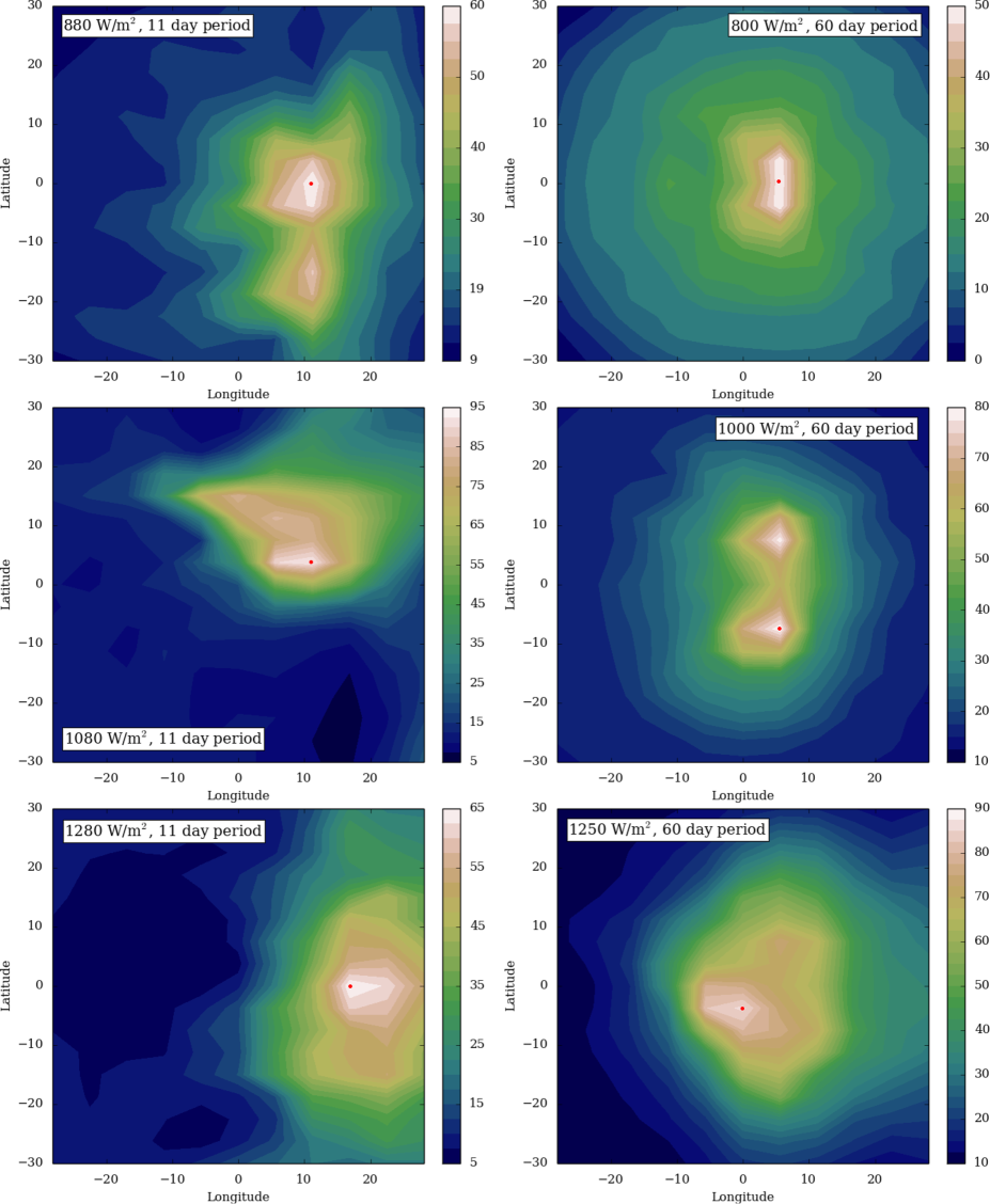
Figure 1: Vertically integrated time averaged over 20 days aerosol opacity in the GCM for an incident of 880W m^-2 and 11 days rotation period (top left), 1080W m^-2 and 11 days rotation period (middle left), 1280W m^-2 and 11 days rotation period (bottom left), 800 W m^-2 and 60 days rotation period (top right), 1080W m^-2 and 60 days rotation period (middle right) and 1250W m^-2 and 60 days rotation period (bottom right). The red dot refers to the position where the initial profiles are extracted.

The position of the maximum cloudiness is close to the equator therefore no Coriolis effect is considered in the CRM runs. To take into account the heating/cooling from the large-scale circulation of the atmosphere, a heating rate profile extracted from GCM runs is added up to the temperature tendency from the physics package, in a similar way as in Lefèvre et al., (2017, 2018), called advection heating rate hereafter. These profiles are time-averaged and constant during the time of the simulations. On tidally-locked planets two circulation regimes prevail: equatorial super-rotating jet or substellar/anti-substellar circulation. The equilibrium depends on the the equatorial Rossby deformation radius (Leconte et al., 2013b, ). Only the effect of the large-scale circulation on the temperature is considered in this study. For the planets considered in our study, i.e. an N₂-dominated atmosphere with a surface temperature around 300 K with a planetary radius close to the Earth, the atmospheric circulation falls into the two regimes. For a 11 days rotation period, the planetary atmosphere is in an equatorial super-rotating jet regime with planetary-scale waves interactions (Showman and Polvani,, 2011; Hammond and Pierrehumbert,, 2018). For a 60 days rotation period, the equatorial Rossby deformation radius exceeds the planetary radius and therefore a planetary Rossby wave would be bounded by this radius, and thus the substellar/anti-substellar circulation dominates the large-scale circulation. This difference in circulation reverberates to differences in the advection heating rates, in particular between 15 and 25 km (see Fig 2), and exhibits the greater efficiency of heat transport for slow rotators. A time-averaged GCM vertical profile of zonal and meridional winds is prescribed.

The general circulation therefore dominates the advection heating in the upper atmosphere while closer to the surface it is the convection. These rates are time-averaged from the GCM simulation, however to avoid any influence from the moist convective scheme used in the GCM physics package and let the resolved convection in the CRM free to equilibrate, the advection heating rate profile is set to a constant value of -1 $\times$ 10^-6 K s^-1 from the surface to approximately 9 km, representative of the cooling of the atmosphere at this altitude. Fig 2-a displays the initial temperature profile (K), Fig 2-b the advection heating rate vertical profile (in 10^-5 K s^-1 units), Fig 2-c the initial zonal wind profile (m s^-1) and Fig 2-d the initial water vapor vertical profile (kg/kg of air). The atmosphere is assumed to be initially cloud-free. The stellar fluxes for the two rotation rates are slightly different to ensure a similar surface temperature which is expected to be the main driver of the convection and a key factor of the organisation of the convection. 3 sets of initial surface temperatures (calculated with the GCM simulations) are considered: 295 K, 305 K and 315 K at the substellar point. As shown in Fig 1 with the red dots, the extracted profile are not at the substellar point and so the surface temperatures differ over a few Kelvins from the reference surface temperature. The surface temperature is free to evolve during the simulation. The bottom boundary is an oceanic surface with a 0.07 albedo. The planetary and atmospheric parameters for the different cases considered are summed-up in Table 1.

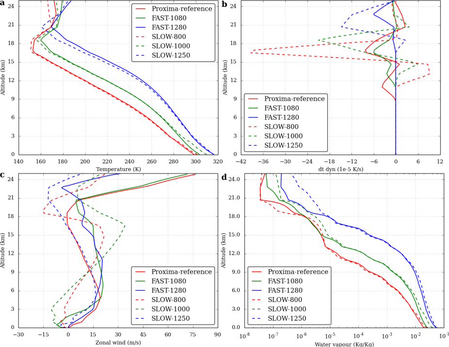
Figure 2: Initial vertical profile of the atmospheric temperature in K (a), advection heating rate in K/s (b), zonal wind in m/s (c) and water vapour in kg/kg of air (d) for the six case of stellar insolations and rotation rates considered in our study (see Table 1). These profiles are time-averaged GCM outputs at the maximum of column water cloud fraction (Fig 1). The constant value of the large-scale from the surface to approximately 9 km is set to 10^-6 K s^-1 (see text).

The horizontal grid size is 1 km over 250 x 250 km to be able to revolve large convective cells, between two and three times the size of the LMD Generic GCM cells at the equator. We use a double periodic domain. The vertical domain extends from the surface to 25 km of altitude, about 900 Pa, to ensure that the convective plumes are able to reach their equilibrium levels. The number of vertical points is set to 80. A Rayleigh sponge layer is set at the top of the domain with a 1 km depth and a damping coefficient of 0.01 s^-1 to avoid spurious reflection of upward-propagating gravity waves (Klemp et al.,, 2008). The different cases are run over about 10 Earth days.

Parameter	Value
Heat Capacity (J K-1)	1000
Surface Pressure (Pa)	105
Composition	N2-dominated, CO2 : 376 ppm, H2O : variable amount (Fig 2)
Obliquity	0
Eccentricity	0
Case	Stellar Type	Incident flux	Rotation period	Gravity
		(W m-2)	(days)	(m s-2)
Proxima b (reference)	M5.5	880	11	10.97
FAST-1080	M5.5	1080	11	10.97
FAST-1280	M5.5	1280	11	10.97
SLOW-800	M2	800	60	13.72
SLOW-1000	M2	1000	60	13.72
SLOW-1250	M2	1250	60	13.72

Table 1: Planetary and atmospheric parameters for the different simulations.

3 Results for the reference simulation

We present in this section the results of our reference simulation, corresponding to the parameters (spectral insolation, mass, rotation rate, etc.) chosen to best reproduce the exoplanet Proxima b (corresponding to the first case in Table 1).

Fig 3 shows three snapshots of resulting vertical wind field (m s ^-1) after about 30h of simulations: a vertical cross-section (a) and a horizontal cross-section at 1 km altitude (c) and 20 km altitude (c). Shallow convection is visible below 3 km with cells between 20 and 50 km of diameter and vertical wind reaching $\pm$ 8 m s^-1, slightly above Earth shallow convection values at the same altitude (Schumacher et al.,, 2015; Giangrande et al.,, 2016). At 2.5 km, the typical vertical wind ranges between $\pm$ 1.5 m s^-1, three times the values at this altitude in Sergeev et al., (2020) study. This difference is due to the thickness of the shallow convection, thicker in the present study. The diameter of these cells is comparable to that of Earth shallow convection cells (Atkinson and Wu Zhang,, 1996). From 5 km to approximately 19 km (about 40 mbar), deep convection occurs with vertical wind reaching up to 40 m s^-1. On Earth, deep convective plumes reach the tropopause at typically 15 km with vertical wind speed up to 20 m s^-1 (Zipser and Lemone,, 1980; Giangrande et al.,, 2016), in some extreme cases the plumes can reach 20 km altitude with vertical up to 50 m^-1 (Dauhut et al.,, 2016). The difference in low altitude vertical velocity with Sergeev et al., (2020) is due to a difference of shallow convection depth in the present study, allowing higher vertical velocity. This difference in tropopause height engenders a higher convective available potential energy (CAPE) and leads to higher vertical velocity. Above 17 km and up to 20 km, tropopause-overshooting convection is visible. For comparison, above the United States only approximately 2 $\%$ of the overshooting convection reaches altitude 3 km above the tropopause (Cooney et al.,, 2018). In the absence of ozone heating in the model, the stratosphere lacks an inversion and is less stable, and could allow more penetration. At 15 km, the vertical wind is dominated by the large cluster (x = 75 ; y = 50) km with a diameter of 50 km, but there are also several smaller plumes with 10 km diameter. The deep convective plumes reaching their top altitude will engender upward and horizontally propagating gravity waves transporting heat and momentum. Such strong convective activity is known to affect Earth’s atmosphere through the quasi-biennal oscillation (QBO) atmospheric feature (Dunkerton,, 1997). Convectively generated gravity waves are thought to take part in similar QBO-like features in Giant-like and Brown Dwarfs atmospheres (Showman et al.,, 2019).

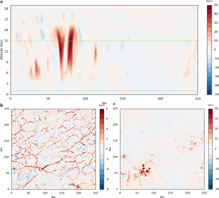
Figure 3: Screenshots after 30h of simulation of the vertical cross section (a) of the vertical wind (m s^-1) and horizontal cross-section of the vertical wind (m s^-1) at 1 km above the surface (b) and at 15 km above the surface (c) for the reference case. The cyan and green lines indicates the altitudes of the two horizontal cross-section, respectively 1 and 15 km. The vertical cross section is at y = 56 km.

This deep convection transports water vapour from 4 km up to the tropopause, leading to water condensation and thus cloud formation. Fig 4 shows a screenshot of a vertical cross section of the water clouds abundance (top) and a vertical cross-section of the water vapour enrichment (bottom), i.e. the relative change regards to the mean water vapor vertical profile.

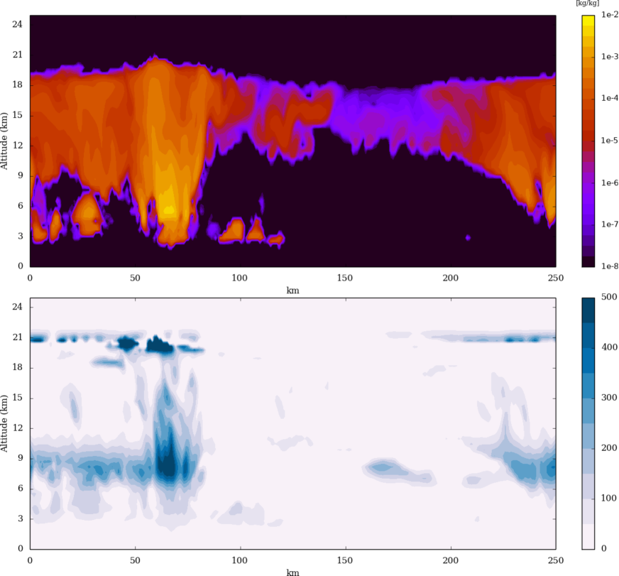
Figure 4: Screenshot of the the vertical cross section of the mixing ratio of water clouds (top) in kg/kg of air and of the water enrichment, i.e. the relative change, in $\%$ (bottom) for the reference case. For clarity the scale of values enrichment is limited at 500 $\%$ but it reach higher values. The vertical cross section is at y = 56 km.

Between 12 (160 mbar) and 18 km, there is the presence of a complete cloud cover, as obtained in past GCMs study Yang et al., (2013). The enrichment of water vapour at x $\sim$ 75 km is related to the large vertical plumes visible in Fig 3a, reaching up to 500 $\%$ enhancement compared to the mean water vapour abundance at this same altitude. The maximum of this enrichment is above 20 km due to convection overshooting with a value as high as 10 000 $\%$ The water is then advected horizontally by winds and visible between 200 and 250 km in the x axis. On Earth the water vapour enrichment at 100 hPa due to overshooting convection can reach up to 300 $\%$ (Herman et al.,, 2017). Fig 5 shows the evolution with time of the stratospheric water vapour content (kg/kg of air). Soon after initialization, there is an abrupt decrease of water vapor due to the water vapour condensation, after the organization of convection the water vapor is transported by the large plume resulting to enrichment visible below 21 km with a maximum of increase by almost a factor 4 around 19 km. This water vapor advected by the convection from the lower atmosphere to the stratosphere is then advected by wind and can condense elsewhere on the planet. Between 21 km and 23 km the atmosphere becomes drier.

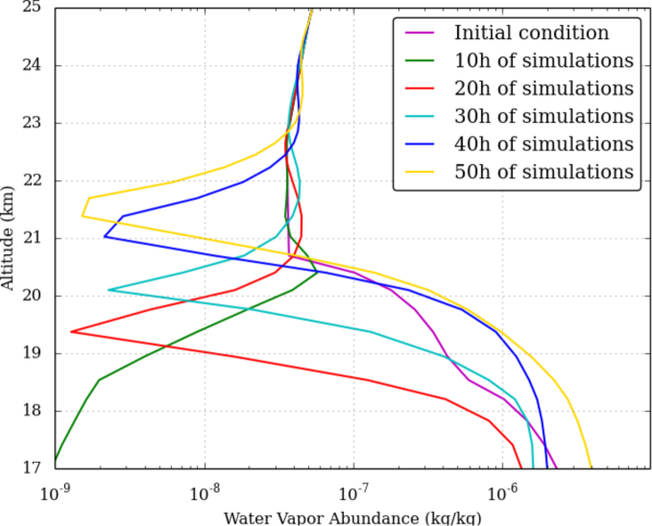
Figure 5: Vertical profile of domain-averaged water vapor content (kg/kg) in the stratosphere at initial condition, after 10 h, 20 h, 30 h, 40 h and 50 h of simulations for the reference case.

Fig 6 displays the cloud fraction for the Proxima standard case. The equivalent of Earth stratocumulus clouds are visible below 5 km and covers about a tenth of the surface, compared to 20$\%$ for stratocumulus above tropics ocean (Eastman et al.,, 2011). Between 12 and 19 km the cloud cover increase up to almost 100 $\%$ as predicted by GCM modelling (Yang et al.,, 2013). Surface rain over the domain is equal to 15 mm/day. Under the deep convective plume, the surface rain reaches 120 mm/day.

The cloud cover is much lower in this CRM study compared to the GCM, especially for the low altitude clouds which will greatly impact the radiation reaching the surface. The cloud fraction in the GCM is non-zero from the surface, with almost 60 $\%$ to about 40 $\%$ at 2 km, whereas for the CRM model the cloud fraction is non-zero from 2 km, where the shallow convection ends. At this altitude the GCM cloud fraction is larger than 45 $\%$. This substantial discrepancy in cloud cover could explain the difference in albedo (discussed hereafter) between the CRM and GCM models and shows the way to deal with the shallow convection. The high cloud layer is quite comparable in depth but at different altitude, 3 km higher for the CRM.

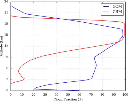
Figure 6: Comparison between the domain-averaged vertical profile of the cloud fraction obtained with the CRM (red) for the reference case and the time average vertical profile of the cloud fraction from the LMD Generic GCM (blue) at the chosen position (see Fig 1).

These clouds impact the fraction of shortwave radiation able to reach the surface but also the longwave infrared thermal emission. Fig 7-a shows the outgoing longwave radiation (OLR) in brightness temperature units (K). The large cluster with a diameter of 150 km – where the OLR reaches a minimum value – corresponds to the vertical plume visible at x $\sim$ 75 km in Fig 3-a. The brightness temperature drops to about 160 K in that structure, corresponding to an altitude of 16 km (Fig 2a). Outside of the cluster the OLR can reach values up to 260 K, equivalent of an altitude of 6 km above the surface. This structure resemble convection aggregation (Wing and Emanuel,, 2014) but is transient, with a lifetime of about 3 hours, typical for a convective structure of that size (Roca et al.,, 2017). After it collapses, an other structure with similar size is emerging at a different location of the 250 x 250km grid. Circular patterns of a few tens of kilometers are also visible. They are associated with the presence of smaller convective plumes. Fig 7-b shows a horizontal cross section of the relative humidity at 8 km. The deep convective cluster is drying the non-convection area, acting like self-aggregation on Earth (Tobin et al.,, 2012).

Fig 7-c shows the corresponding Bond albedo map and Fig 7-d shows the corresponding vertically integrated water cloud (Kg m^-2). Albedo can reach values from 0.05 in cloud-free regions up to 0.34 in the regions corresponding with the positions of high altitude convective plumes, where there is the largest amount of clouds (reaching up to 5 kg m^-2 in the column). The low altitude stratocumulus clouds contribute for a significant part of the high albedo values as visible at x = 160 km with less than 1 Kg m^-2 in the column. The domain averaged value of the Bond albedo is 0.06 whereas the GCM Bond albedo is 0.32. This is explained firstly by the fact that the cloud coverage ($\sim$ 10$\%$ for low altitude stratocumulus clouds) is relatively low; and secondly by the fact that the cloud-free regions have a very low bond albedo. The latter stems from the fact that the albedo of the ocean surface is low (0.07), that the Rayleigh scattering is inefficient around a cool star such as Proxima Cen, and that the water vapour-enriched atmosphere absorbs efficiently near-infrared emission from the star. A similar reduction of the bond albedo is also observed in the 1-D cloud-free simulations of Kopparapu et al., (2013) (see Fig. 6a, calculated for a surface albedo of 0.3).

The maximum bond albedo value in the CRM, corresponding to the large convective cluster, is comparable to the mean GCM bond albedo at the substellar point. This substantial discrepancy could be explained by the significant difference in low altitude clouds fraction between the CRM and GCM models and difference of shallow convection. This value of albedo can be compared to the TOGA-COARE case with Sun spectra in the Appendix A, where the albedo inside the deep convective plume is around 0.6 whereas the albedo is about 0.1 in the cloud-free region. The low value of the overall albedo is much smaller than previous GCM previsions (Yang et al.,, 2013; Yang et al., 2019b, ), which reflects the fact that outside deep convective layers where the albedo is close to previous GCM studies, the areas of low cloud fraction have low cloud albedo and therefore aggregation of convection, even transient like in the study, can have a strong effect on the overall albedo due to the low mass star spectra.

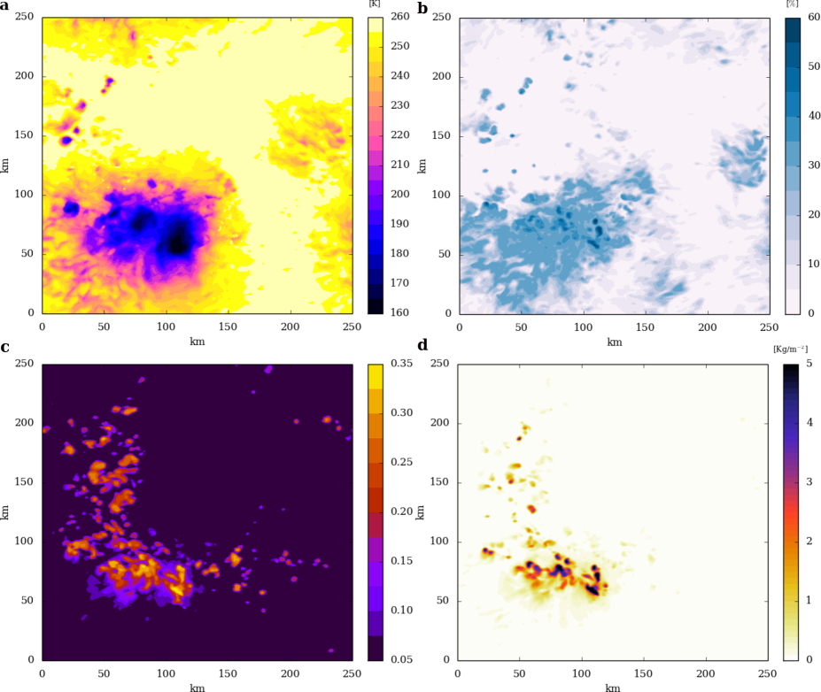
Figure 7: Screenshot of the OLR brightness temperature in K (a), the relative humidity at 8 km (b), the bond albedo (c) and vertically integrated water clouds abundance in Kg m^-2 (d) for an incident stellar flux of 880 W m^-2 and a 11 days rotation period.

In addition to its synchronous rotation, another specificity of Proxima Centauri b compared to Earth is the spectra of its host star. Proxima Centauri is an M5.5 type star (Bessell,, 1991) with an effective temperature of 3050 K with a maximum of the emission spectra around 1 $\mu$m (Pavlenko et al.,, 2017). This shift towards the infrared is expected to impact the absorption of the stellar spectra by the atmosphere, especially by water. Fig 8 shows vertical profiles of the stellar heating (W m^-2) for two water cloud features for both the TOGA-COARE case (blue line) with sun spectra and the Proxima Centauri b reference case with M-star spectra (red line).

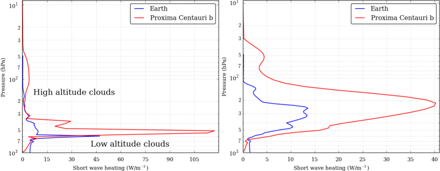
Figure 8: Vertical profiles of incident stellar heating (in W m^-2, per atmospheric layer). The red lines are for Proxima Centauri b reference case and the blue lines are for the TOGA-COARE case. The left figure is for the case of the presence of both high altitude clouds and low altitude clouds and the right panel is for the case of deep convection.

The two water cloud features displayed are high altitude and low altitude clouds and deep convection. On the left figure for Earth, high clouds absorb solar heating around 1.5 $\times$ 10² hPa while the absorption by the low altitude clouds occurs at 6 $\times$ 10² hPa. For Proxima Centauri b, high clouds absorb solar heating between 2 $\times$ 10² hPa and 4 and 7 $\times$ 10¹ hPa with a maximum at 1 $\times$ 10² hPa and the absorption of the low altitude clouds occurs at 5 $\times$ 10² hPa for the reference case. The short wave heating by the low clouds on Proxima Centauri b is almost three times stronger that Earth, shielding more efficiently the surface from the incoming stellar radiation. For the deep convection case (right figure), for both Proxima Centauri b and Earth the short wave heating is absorb on a larger vertical scale, the heating is also stronger for Proxima Centauri b, more than three times the one on Earth. A larger part of the energy coming from the host star is absorbed by the atmosphere gas and clouds, and therefore even with a lower overall albedo, the energy reaching the surface is lower for a planet orbiting of M-star than a Sun-like star (for an Earth-like atmosphere).

4 Impact of the incident flux

Fig 9 shows the comparison of the cloud coverage for the reference case with the FAST-1080 and FAST-1280 cases (all with a 11 days rotation period). In all the three cases, there is a high-altitude cloud layer. The altitude of this layer is determined by the thermal structure. The tropopause increases with the stellar flux, with a value of 17 km (50 hPa) for the standard case, 19 km (32 hPa) for the FAST-1080 and 21 km (20 hPa) for the FAST-1280 case (see Fig 2a). The thickness of this high-altitude cloud layer decreases with the increase of the incident flux. This inverted trend is due to the low altitude clouds. The increasing stellar flux engender a thicker shallow convection, from around 3.0 km for the reference case to 5.6 km for the FAST-1280 case, leading to more extented vertical mixing of the water vapor in the shalow convection. Domain-averaged value for the standard case is 8 x 10^-3 kg/kg, 1.1 x 10^-2 kg/kg for the FAST-1080 case and 2.3 x 10^-2 kg/kg for the FAST-1280 case. This increase in water vapor by the shallow convection triggers more condensation, leading to an increase of the low-altitude clouds coverage, reaching up to 60$\%$ for the FAST-1280 case.

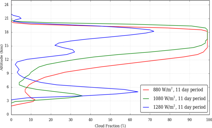
Figure 9: Comparison of the domain-averaged cloud fraction for the reference case (Top), FAST-1080 (Middle) and FAST-1280 (Bottom) cases.

Fig 10 shows the atmospheric albedo (left) and the OLR brightness temperature (K) for the reference case (Top), FAST-1080 (Middle) and FAST-1280 (Bottom) cases. One noticeable behaviour is the increase of both the atmospheric albedo and the OLR with the increase of the stellar flux. The structure of the albedo map for the standard case is dominated by the high cloud layer visible in the OLR map. For the FAST-1080 case, the contribution of high-altitude clouds is visible in the center of the map but the low-altitude cloud layer is dominating with small patchy structures. The contribution of low-altitude clouds is even more important for the FAST-1280 case where the contribution of the high-altitude clouds, visible on the OLR map, is barely noticeable.

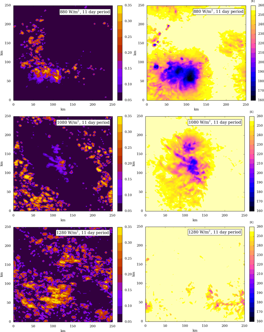
Figure 10: Snaphots of albedo (Left) and OLR brightness temperature in K (Right) for Proxima b (Top), FAST-1080 (Middle) and FAST-1280 (Bottom) cases.

With the increase of the stellar flux, the thermal structure of the atmosphere changes with an increase of the tropopause height as well as an increase of the atmospheric water vapor mixing ratio. This increase of stellar flux induces a thicker shallow convection leading to an increase of the low altitude cloud layer coverage. This increase of the low altitude clouds engender an increase of the atmospheric albedo and a stronger short wave cloud radiative feedback. This temperature trend is consistent with anvil cloud fraction SST dependence on Earth (Bony et al.,, 2016), where an increase of the SST reduces the cloud fraction.

Simulations with initial surface temperature around 350 K, corresponding to incoming stellar flux of 1500 and 1610 W m$m^{-2}$ for the FAST and SLOW cases respectively, was conducted but not shown here. The abundance of water vapor in the atmosphere reaches values superior to 20%, going over the dilute regime, therefore a condensation of water vapor would lead to a significant pressure change not taken into account by the model. To be able to study such temperatures range changes need to be carried out to take into the non-dilute regime.

5 Impact of the rotation period

The rotation period has an important impact on the circulation of a planetary atmosphere. The strength of the Coriolis force dictates the extend of the thermally direct latitudinal circulations and the surface temperature distribution, which drives atmospheric circulation (Pierrehumbert,, 2010). From Fig 2-a, we observe that the thermal structures and water vapour vertical distributions are similar for the slow and fast rotation cases (for a given surface temperature), whereas the advection heating rates have different behaviour (Fig 2-b). For the SLOW cases, the profile of advection heating rates for the 3 cases of solar insolation have similar behaviour with positive values region between 12 and 18 km and above a strong negative values region between 16 and 21 km. On the other hand, for the FAST cases the advection heating rates have only negative below 21 km.

Fig 11 shows the comparison of the cloud coverage for the 6 cases studied in our work: the reference case, FAST-1080 and FAST-1280 with a 11 days rotation period and SLOW-800, SLOW-1000 and FAST-1250 with a 60 days rotation period. The height of the tropopause is very similar for the two rotation periods but the advection heating rates are quite different with stronger values for the 60 days rotation rate. For the 6 cases, there is a high-altitude cloud layer thinner with increasing stellar flux as described in the previous section. The depth of this cloud layer also increases with the rotation rate. The high-altitude cloud layer is about 1.5 km thicker for the SLOW-800 compared to the reference case, 2 km thicker for the SLOW-1000 case compared to the FAST-1080. For the SLOW-1250, this layer is not only thicker but it reaches higher cloud fraction values. The low-altitude cloud coverage is very similar for the four highest incident stellar flux cases whereas for the two lowest there is a significant difference with the rotation period. The low altitude cloud coverage of the SLOW-800 case is almost four times the coverage of the reference case. The altitude of the lower cloud deck is varying with the incident flux but also with the rotation period. For the 60 days cases, the top of the shallow convective layer is lower, especially at high stellar flux. This effect increases the albedo and can be attribute to the thicker high altitude cloud layer absorbing and reflecting more incident stellar flux.

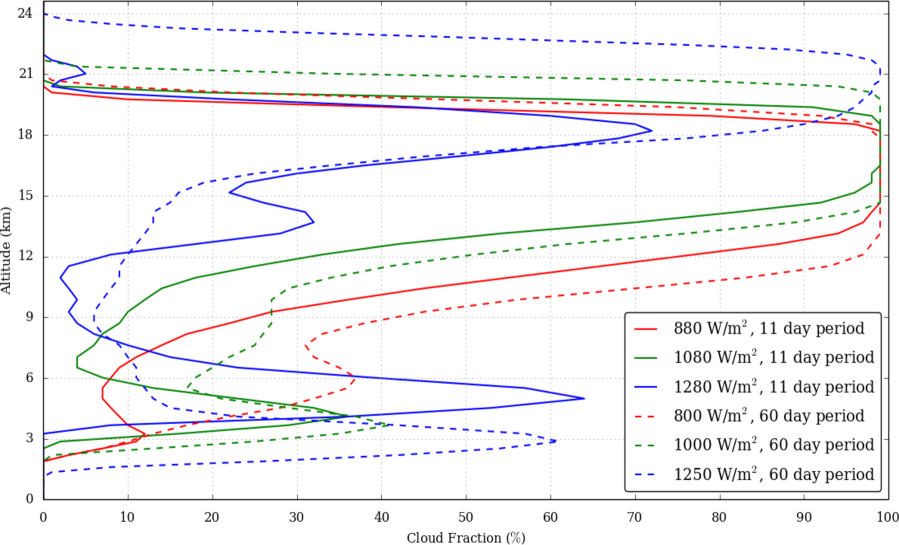
Figure 11: Comparison of the domain-averaged cloud fraction for the SLOW-800 (Top), SLOW-1000 (Middle) and SLOW-1250 (Bottom) cases.

Fig 12 shows the albedo (left) and the OLR brightness temperature for SLOW-1000 (Top), SLOW-1000 (Middle) and SLOW-1250 (Bottom) cases. Compared to Figure 10, the OLR brightness temperature is lower for the 60 days rotation period than for the similar 11 days rotation case. For example, the large-scale structure visible in the Figure 12 (bottom right) for the SLOW-1250 has a stronger OLR flux, i.e. a smaller brightness temperature, than the large-scale structure visible in the Figure 10 (bottom right) for the FAST-1280 case. This is due to the fact that the high-altitude clouds is more developed for the 60 days rotation period and that the updrafts are stronger. The increase of low clouds albedo with the with increase of surface temperature is also noticeable with the a 60-days rotation rate as for a 11-days rate.

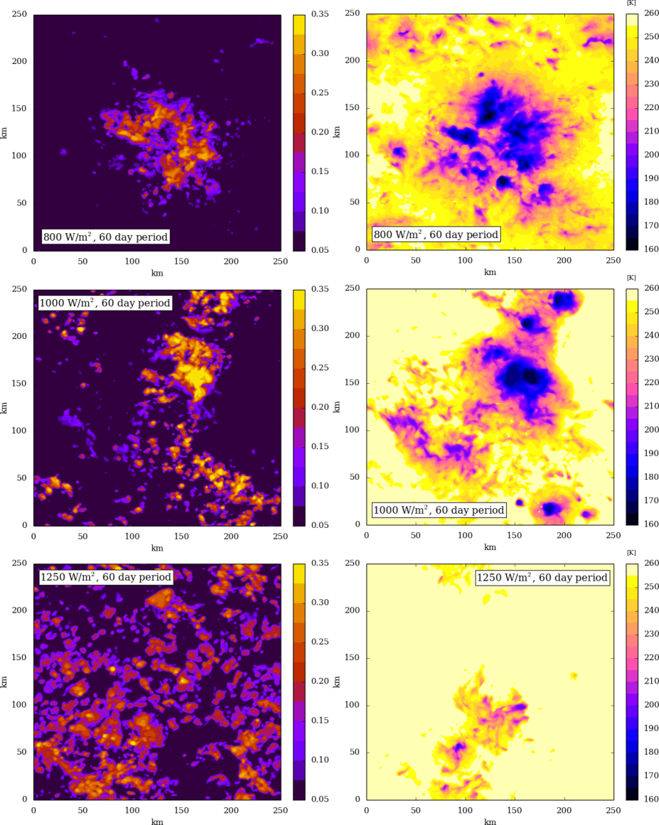
Figure 12: Snaphots of albedo (Left) and OLR brightness temperature in K (Right) for SLOW-800 (Top), SLOW-1000 (Middle) and SLOW-1250 (Bottom) cases.

In summary, the increase of the rotation period engenders a change of circulation regime leading to a different behaviour of the advection heating rate in altitude. This increase of the high altitude cloud layer thickness is linked to the vertical structure of the profile of advection heating rates between 12 and 21 km. This structure with positive values followed by negative of heating rates will trigger additional convective activity in this region. The increased thickness of the altitude cloud layer correspond to the region where this triggering takes place, between 12-19 km for the SLOW-800 case, 15-20 km for the SLOW-1000 case and 18-24 km for the SLOW-1250 case. This triggering will increase the convective activity and the vertical transport of water vapor in this region, and therefore engender a thicker cloud layer. With this change in high-altitude clouds, a decrease of shallow convective layer is occurring leading to an increase of the Bond albedo and cloud feedback.

6 Discussions

Fig 13 shows the comparison of the domain-averaged Bond albedo for the 6 cases as a function of the incident stellar flux. The trends discussed in Sections 4 and 5 are visible. The bond albedo is increasing of about 20% with the increasing flux and is increasing of between 5 and 10% with increasing rotation period. The study of Yang et al., (2013) found a similar trend in the increase of bond albedo with insolation: between stellar fluxes of 1000 and 1200 W m², the bond albedo increases by 7%, although with much higher values around 0.45. Using a GCM with a high-resolution zoom in the substellar region, Sergeev et al., (2020) studied the convection on tidally-locked Earth-like planets. A notable discrepancy is the fact that the albedo inside the high-resolution area is higher than with the low-resolution GCM in Sergeev et al., (2020), whereas in this study the albedo of the CRM is lower than in the GCM. The main noticeable difference between the two models is that in Sergeev et al., (2020), the large-scale forcing is given by the GCM fields (temperature, water content, winds, …) in real-time whereas in this study the large-scale forcing is represented by a single time averaged vertical profile in temperature fixed in time and space. This difference in handling the large-scale forcing could lead to a difference of the shallow convection depth and therefore a difference in albedo. The aggregation of convection showed in Section 3, and not seen in Sergeev et al., (2020) study, is also one factor of this albedo discrepancy. These differences between the two models call for more convection resolving modelling in such atmospheric environment leading to an intercomparison, possibly in the same way the THAI GCM intercomparison for exoplanets (Fauchez et al.,, 2019) was carried out, in order to improve the understanding of convection processes in exoplanetary environments.

The model does not make the difference between liquid water cloud and water ice cloud. The impact of the general circulation is represented in the model by a constant heating rate profiles, a water vapor tendency profile could be imposed to the domain to take into account the water vapor advection near the substellar point. The temperature impact of the general circulation is represented with a constant tendency profile close to the surface, a more realistic approach with a time-dependent profile could improve the physical representation of the advection near the substellar point. Another improvement of the model will be to take into account ocean circulation. Del Genio et al., (2019) showed the impact of such circulation on the SST and the clouds self-aggregation (Müller and Hohenegger,, 2020) and how SST anomalies can favor the aggregation of convection (Shamekh et al.,, 2020). The oceanic circulation is also believed to have a significant impact on the atmospheric circulation, with a planetary heat transport dominated by the ocean at moderate incident stellar fluxes and by the atmosphere near the inner edge of the habitable zone Yang et al., 2019a . This is assuming an oceanic surface, the case of continental surface also needs to be carried out.

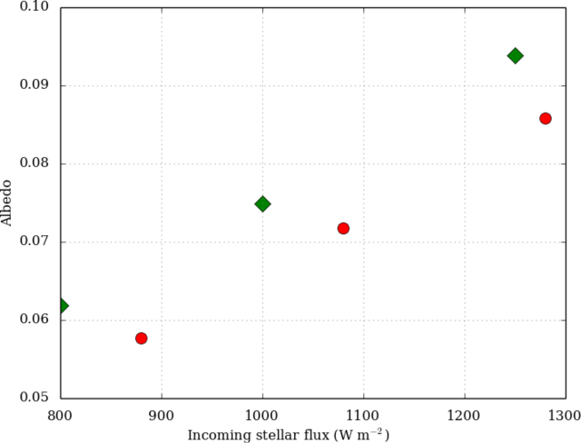
Figure 13: Domain-averaged bond albedo as a function of the incident stellar flux (in W m^-2) for the CRM. Diamonds are for SLOW cases and circles for the FAST cases.

7 Conclusion

We presented the LMD Generic CRM coupled to realistic radiative transfer and a non-Earth based cloud microphysics model. This versatile model is able to resolve realistic Earth tropics convection as well as to perform in extreme insolation conditions such as those experienced on tidally-locked planetary atmospheres such as Proxima b. In this study, we presented the results of resolved convection simulations of the Proxima-b environment assuming an Earth-like atmospheric composition, for several incident stellar fluxes and rotation periods.

For the standard case, organised convection is resolved with a shallow convection of 2.5 km in depth and 60 km in diameter. Convective clouds are present reaching up to 20 km of altitude and 150 km in diameter. Inside this strong updraft, vertical velocity can reach 40 m s^-1 with surface rain values of 120 mm/day under. A thick 100 $\%$ cloud cover between 12 and 18 km is present. The convective clouds transport water vapor from the surface to the troposphere. Around 19 km, this enrichment of water vapor is maximal with a four-fold increase compared to initial conditions.

Simulations with higher stellar fluxes and slower rotation rate were conducted. The bond albedo is sensitive to these two physical parameters. The albedo increases when the stellar flux increases, from an increase of the low altitude cloud fraction and a decrease of the depth of the high-altitude cloud layer, overall increasing the albedo. The decrease of the rotation rate has the effect to change the general circulation especially between 20 and 30 km. This difference of circulation triggers a thicker high-altitude cloud layer thus increasing the bond albedo.

The short wave cloud feedback resolved by the model is lower than the cloud feedback predicted by previous GCM simulations (Yang et al.,, 2013; Yang et al., 2019b, ). The shallow convection and low altitude clouds are different in the two models, in the CRM the shallow convection is thicker and the cloud coverage of low-altitude clouds is lower leading to a smaller albedo. The high altitude cloud coverage is similar between the two models. While the CRM exhibits a small overestimation

of the shallow convection height, this discrepancy between the cloud coverage obtained with this model and the cloud coverage from the LMD GCM is suggesting that the moist convection parametrization scheme does not handle correctly the convection and cloud formation of the near surface area. This study will be used to calibrate a more realistic convection representation such as a thermal plume model (Rio and Hourdin,, 2008; Rio et al.,, 2010).

The simulations show signs of organized convection with cellular cluster of about 150 km in diameter. However the domain size could be one limit to the aggregation of convection. In such incoming stellar environment, it is important to consider the albedo effect of aggregation of convection . Simulations with a larger horizontal domain should be performed to fully understand the mechanisms of that phenomenon (Bretherton and Khairoutdinov,, 2015; Wing and Emanuel,, 2014).

The high velocity inside the largest convective clouds with water cycle is the perfect environment for the occurrence of lightning. NOx and HOx chemistry could therefore be triggered and have an impact on stellar absorption (Ardaseva et al.,, 2017)

and on HCN production rate, a key feedstock of life’s building blocks (Rimmer and Rugheimer,, 2019). To investigate these effects, improvement is needed into the representation of the water cycle in the microphysical model that would need to handle separately liquid water cloud and ice water cloud as well as the inclusion of graupel.

The simulations here are for an atmospheric composition close to the Earth. Thanks to the versatility of the model the impact of different composition on the cloud coverage will be explored, for example the impact of CO₂ abundance, thought to decrease stratocumulus cloud coverage (Schneider et al.,, 2019). Water vapour has been detected on the habitable-zone super-Earth exoplanet K2-18 b in an atmosphere thought to be hydrogen-rich (Benneke et al.,, 2019; Tsiaras et al.,, 2019). The difference of molecular mass between hydrogen and water will engender compositional buoyancy that will impact the convection (Leconte et al.,, 2017; Charnay et al.,, 2021). Another compositional effect that will be explored is the non-dilute convection regime (Ding and Pierrehumbert,, 2016), where the condensing component is the principal or non negligible species.

Appendix A TOGA-COARE modeling

As stated in Section 2 the model presented in this study was tested with Earth tropics convection data from the TOGA-COARE campaign. The temperature, pressure, water vapor and wind profiles are taken from the measurement campaign. Advection heating and water vapour advection are also taken account. The surface temperature is set up at the beginning of the simulations and then is free to evolve during the simulation. With similar settings that those described in Section 2 with a Sun spectrum and a diurnal cycle, the model resolves convection showed at Fig 14 after 6 Earth days of simulation.

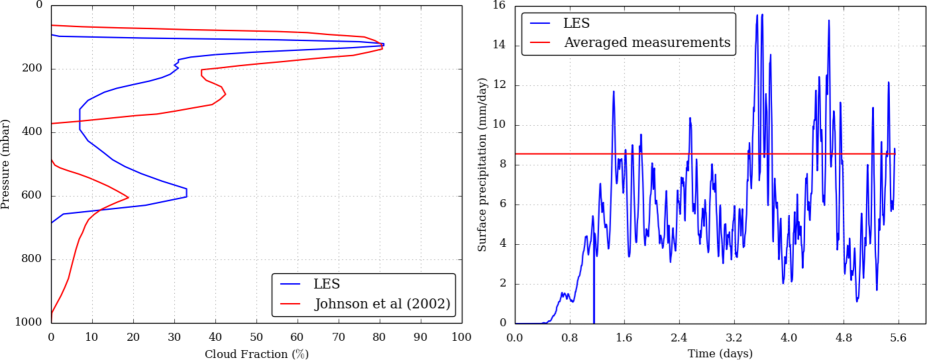
Figure 14: Left : average cloud fraction resolved by the model (CRM) and by Johnson et al., (2002). Right : surface rain(mm/day) over the whole domain (CRM) and averaged measurements.

The cloud fraction (left) is calculated using Xu and Krueger, (1991) formulations to be compared to Johnson et al., (2002). The overall behaviour is very similar, however the low altitude clouds are slightly overestimated by the model and the high altitude clouds are a little underestimated. The height of the cloud bottom boundary, about 750 hPa, is as well overestimated compared to similar modeling, about 950 hPa (Daleu et al.,, 2015). The surface rain resolved by the model is close to the average of models from Johnson et al., (2002) and Wang et al., (2013). However the model is not designed to reproduce extreme events, such as strong sudden increase of a domain average surface rain over 40 mm/day (Wang et al.,, 2013). This model is suited to exhibits realistic behaviour for Earth tropics convection.

References

- Anglada-Escudé et al., (2016) Anglada-Escudé, G., Amado, P. J., Barnes, J., Berdiñas, Z. M., Butler, et al. (2016). A terrestrial planet candidate in a temperate orbit around Proxima Centauri. Nature, 536:437–440.
- Ardaseva et al., (2017) Ardaseva, A., Rimmer, P. B., Waldmann, I., Rocchetto, M., Yurchenko, S. N., et al. (2017). Lightning chemistry on Earth-like exoplanets. Monthly Notices of the Royal Astronomical Society, 470(1):187–196.
- Atkinson and Wu Zhang, (1996) Atkinson, B. W. and Wu Zhang, J. (1996). Mesoscale shallow convection in the atmosphere. Reviews of Geophysics, 34:403–431.
- Auclair-Desrotour et al., (2019) Auclair-Desrotour, P., Leconte, J., and Mergny, C. (2019). Generic frequency dependence for the atmospheric tidal torque of terrestrial planets. Astronomy Astrophysics, 624:A17.
- Benneke et al., (2019) Benneke, B., Wong, I., Piaulet, C., Knutson, H. A., Crossfield, I. et al. (2019). Water Vapor on the Habitable-Zone Exoplanet K2-18b. arXiv e-prints, page arXiv:1909.04642.
- Bessell, (1991) Bessell, M. S. (1991). The Late M Dwarfs. Astronomical Journal, 101:662.
- Bolmont et al., (2016) Bolmont, E., Libert, A.-S., Leconte, J., and Selsis, F. (2016). Habitability of planets on eccentric orbits: Limits of the mean flux approximation. Astronomy & Astrophysics, 591:A106.
- Bonfils et al., (2018) Bonfils, X., Astudillo-Defru, N., Díaz, R., Almenara, J.-M., Forveille, T., et al. (2018). A temperate exo-Earth around a quiet M dwarf at 3.4 parsec. Astronomy Astrophysics, 613:A25.
- Bony et al., (2016) Bony, S., Stevens, B., Coppin, D., Becker, T., Reed, K. A., et al. (2016). Thermodynamic control of anvil cloud amount. Proceedings of the National Academy of Science, 113(32):8927–8932.
- Boucher et al., (1995) Boucher, O., Le Treut, H., and Baker, M. B. (1995). Precipitation and radiation modeling in a general circulation model: Introduction of cloud microphysical processes. Journal of Geophysical Research: Atmospheres, 100:16.
- Bretherton and Khairoutdinov, (2015) Bretherton, C. S. and Khairoutdinov, M. F. (2015). Convective self-aggregation feedbacks in near-global cloud-resolving simulations of an aquaplanet. Journal of Advances in Modeling Earth Systems, 7(4):1765–1787.
- Charnay et al., (2013) Charnay, B., Forget, F., Wordsworth, R., Leconte, J., Millour, E., et al. (2013). Exploring the faint young Sun problem and the possible climates of the Archean Earth with a 3-D GCM. Journal of Geophysical Research (Atmospheres), 118(18).
- (13) Charnay, B., Meadows, V., and Leconte, J. (2015a). 3D Modeling of GJ1214b’s Atmosphere: Vertical Mixing Driven by an Anti-Hadley Circulation. The Astrophysical Journal, 813(1):15.
- (14) Charnay, B., Meadows, V., Misra, A., Leconte, J., and Arney, G. (2015b). 3D Modeling of GJ1214b’s Atmosphere: Formation of Inhomogeneous High Clouds and Observational Implications. The Astrophysical Journal Letters, 813(1):L1.
- Charnay et al., (2021) Charnay, B., Blain, D., Bézard, B., Leconte, J., Turbet, M., et al. (2021). Formation and dynamics of water clouds on temperate sub-Neptunes: the example of K2-18b. Astronomy & Astrophysics, 646:A171.
- Cooney et al., (2018) Cooney, J. W., Bowman, K. P., Homeyer, C. R., and Fenske, T. M. (2018). Ten Year Analysis of Tropopause-Overshooting Convection Using GridRad Data. Journal of Geophysical Research (Atmospheres), 123(1):329–343.
- Daleu et al., (2015) Daleu, C. L., Plant, R. S., Woolnough, S. J., Sessions, S., Herman, M. J., et al. (2015). Intercomparison of methods of coupling between convection and large-scale circulation: 1. Comparison over uniform surface conditions. Journal of Advances in Modeling Earth Systems, 7(4):1576–1601.
- Dauhut et al., (2016) Dauhut, T., Chaboureau, J.-P., Escobar, J., and Mascart, P. (2016). Giga-LES of Hector the Convector and Its Two Tallest Updrafts up to the Stratosphere. Journal of Atmospheric Sciences, 73:5041–5060.
- Deardorff, (1972) Deardorff, J. W. (1972). Numerical Investigation of Neutral and Unstable Planetary Boundary Layers. Journal of Atmospheric Sciences, 29:91–115.
- Del Genio et al., (2019) Del Genio, A. D., Way, M. J., Amundsen, D. S., Aleinov, I., Kelley, M., et al. T. L. (2019). Habitable Climate Scenarios for Proxima Centauri b with a Dynamic Ocean. Astrobiology, 19(1):99–125.
- Ding and Pierrehumbert, (2016) Ding, F. and Pierrehumbert, R. T. (2016). Convection in Condensible-rich Atmospheres. The Astrophysical Journal, 822(1):24.
- Dunkerton, (1997) Dunkerton, T. J. (1997). The role of gravity waves in the quasi-biennial oscillation. Journal of Geophysical Research, 102:26053–26076.
- Eastman et al., (2011) Eastman, R., Warren, S. G., and Hahn, C. J. (2011). Variations in Cloud Cover and Cloud Types over the Ocean from Surface Observations, 1954-2008. Journal of Climate, 24(22):5914–5934.
- Edson et al., (2011) Edson, A., Lee, S., Bannon, P., Kasting, J. F., and Pollard, D. (2011). Atmospheric circulations of terrestrial planets orbiting low-mass stars. Icarus, 212:1–13.
- Eymet et al., (2016) Eymet, V., Coustet, C., and Piaud, B. (2016). kspectrum: an open-source code for high-resolution molecular absorption spectra production. In Journal of Physics Conference Series, volume 676 of Journal of Physics Conference Series, page 012005.
- Fauchez et al., (2019) Fauchez, T., Turbet, M., Wolf, E. T., Boutle, I., Way, M. J., et al. (2019). Trappist-1 habitable atmosphere intercomparison (thai). motivations and protocol. Geoscientific Model Development Discussions, 2019:1–15.
- Forget et al., (2013) Forget, F., Wordsworth, R., Millour, E., Madeleine, J.-B., Kerber, L., et al. (2013). 3D modelling of the early martian climate under a denser CO2 atmosphere: Temperatures and CO2 ice clouds. Icarus, 222:81–99.
- Giangrande et al., (2016) Giangrande, S. E., Toto, T., Jensen, M. P., Bartholomew, M. J., Feng, Z., et al. (2016). Convective cloud vertical velocity and mass-flux characteristics from radar wind profiler observations during GoAmazon2014/5. Journal of Geophysical Research (Atmospheres), 121(21):12,891–12,913.
- Gillon et al., (2017) Gillon, M., Triaud, A. H. M. J., Demory, B.-O., Jehin, E., Agol, E., et al. (2017). Seven temperate terrestrial planets around the nearby ultracool dwarf star TRAPPIST-1. Nature, 542:456–460.
- Grabowski, (2001) Grabowski, W. W. (2001). Coupling Cloud Processes with the Large-Scale Dynamics Using the Cloud-Resolving Convection Parameterization (CRCP). Journal of Atmospheric Sciences, 58(9):978–997.
- Grabowski and Moncrieff, (2002) Grabowski, W. W. and Moncrieff, M. W. (2002). Large-scale organization of tropical convection in two-dimensional explicit numerical simulations: Effects of interactive radiation. Quarterly Journal of the Royal Meteorological Society, 128(585):2349–2375.
- Hammond and Pierrehumbert, (2018) Hammond, M. and Pierrehumbert, R. T. (2018). Wave-mean Flow Interactions in the Atmospheric Circulation of Tidally Locked Planets. The Astrophysical Journal, 869(1):65.
- Haqq-Misra et al., (2018) Haqq-Misra, J., Wolf, E. T., Joshi, M., Zhang, X., and Kopparapu, R. K. (2018). Demarcating Circulation Regimes of Synchronously Rotating Terrestrial Planets within the Habitable Zone. The Astrophysical Journal, 852(2):67.
- Held et al., (1993) Held, I. M., Hemler, R. S., and Ramaswamy, V. (1993). Radiative-convective equilibrium with explicit two-dimensional moist convection. Journal of Atmospheric Sciences, 50(23):3909–3927.
- Herman et al., (2017) Herman, R. L., Ray, E. A., Rosenlof, K. H., Bedka, K. M., Schwartz, M. J., et al. (2017). Enhanced stratospheric water vapor over the summertime continental United States and the role of overshooting convection. Atmospheric Chemistry & Physics, 17(9):6113–6124.
- Johnson et al., (2002) Johnson, D. E., Tao, W.-K., Simpson, J., and Sui, C.-H. (2002). A Study of the Response of Deep Tropical Clouds to Large-Scale Thermodynamic Forcings. Part I: Modeling Strategies and Simulations of TOGA COARE Convective Systems. Journal of Atmospheric Sciences, 59:3492–3518.
- Kasting et al., (1993) Kasting, J. F., Whitmire, D. P., and Reynolds, R. T. (1993). Habitable Zones around Main Sequence Stars. Icarus, 101:108–128.
- Kikuchi and Wang, (2008) Kikuchi, K. and Wang, B. (2008). Diurnal Precipitation Regimes in the Global Tropics*. Journal of Climate, 21(11):2680.
- Kirkpatrick et al., (2012) Kirkpatrick, J. D., Gelino, C. R., Cushing, M. C., Mace, G. N., Griffith, R. L., et al. (2012). Further Defining Spectral Type “Y” and Exploring the Low-mass End of the Field Brown Dwarf Mass Function. The Astrophysical Journal, 753(2):156.
- Klemp et al., (2008) Klemp, J. B., Dudhia, J., and Hassiotis, A. D. (2008). An Upper Gravity-Wave Absorbing Layer for NWP Applications. Monthly Weather Review, 136(10):3987.
- Kopparapu et al., (2013) Kopparapu, R. K., Ramirez, R., Kasting, J. F., Eymet, V., Robinson, T. D., et al. (2013). Habitable Zones around Main-sequence Stars: New Estimates. The Astrophysical Journal, 765(2):131.
- Kopparapu et al., (2016) Kopparapu, R. k., Wolf, E. T., Haqq-Misra, J., Yang, J., Kasting, J. F., et al. (2016). The Inner Edge of the Habitable Zone for Synchronously Rotating Planets around Low-mass Stars Using General Circulation Models. The Astrophysical Journal, 819:84.
- (43) Leconte, J., Forget, F., Charnay, B., Wordsworth, R., and Pottier, A. (2013a). Increased insolation threshold for runaway greenhouse processes on Earth-like planets. Nature, 504:268–271.
- (44) Leconte, J., Forget, F., Charnay, B., Wordsworth, R., Selsis, F., et al. (2013b). 3D climate modeling of close-in land planets: Circulation patterns, climate moist bistability, and habitability. Astronomy & Astrophysics, 554:A69.
- Leconte et al., (2017) Leconte, J., Selsis, F., Hersant, F., and Guillot, T. (2017). Condensation-inhibited convection in hydrogen-rich atmospheres . Stability against double-diffusive processes and thermal profiles for Jupiter, Saturn, Uranus, and Neptune. Astronomy & Astrophysics, 598:A98.
- Lefèvre et al., (2018) Lefèvre, M., Lebonnois, S., and Spiga, A. (2018). Three-Dimensional Turbulence-Resolving Modeling of the Venusian Cloud Layer and Induced Gravity Waves: Inclusion of Complete Radiative Transfer and Wind Shear. Journal of Geophysical Research (Planets), 123:2773–2789.
- Lefèvre et al., (2017) Lefèvre, M., Spiga, A., and Lebonnois, S. (2017). Three-dimensional turbulence-resolving modeling of the Venusian cloud layer and induced gravity waves. Journal of Geophysical Research (Planets), 122:134–149.
- Lefèvre et al., (2020) Lefèvre, M., Spiga, A., and Lebonnois, S. (2020). Mesoscale modeling of Venus’ bow-shape waves. Icarus, 335:113376.
- Lilly, (1962) Lilly, D. K. (1962). On the numerical simulation of buoyant convection. Tellus, 14(2):148–172.
- Lipps and Hemler, (1986) Lipps, F. B. and Hemler, R. S. (1986). Numerical Simulation of Deep Tropical Convection Associated with Large-Scale Convergence. Journal of Atmospheric Sciences, 43:1796–1816.
- Lipps and Hemler, (1988) Lipps, F. B. and Hemler, R. S. (1988). Numerical Modeling of a Line of Towering Cumulus on Day 226 of GATE. Journal of Atmospheric Sciences, 45:2428–2444.
- Lovis et al., (2017) Lovis, C., Snellen, I., Mouillet, D., Pepe, F., Wildi, F., et al. (2017). Atmospheric characterization of Proxima b by coupling the SPHERE high-contrast imager to the ESPRESSO spectrograph. Astronomy Astrophysics, 599:A16.
- Moeng et al., (2007) Moeng, C., Dudhia, J., Klemp, J., and Sullivan, P. (2007). Examining Two-Way Grid Nesting for Large Eddy Simulation of the PBL Using the WRF Model. Monthly Weather Review, 135(6):2295–2311.
- Muller and Held, (2012) Muller, C. J. and Held, I. M. (2012). Detailed Investigation of the Self-Aggregation of Convection in Cloud-Resolving Simulations. Journal of Atmospheric Sciences, 69(8):2551–2565.
- Müller and Hohenegger, (2020) Müller, S. K. and Hohenegger, C. (2020). Self-aggregation of convection in spatially varying sea surface temperatures. Journal of Advances in Modeling Earth Systems, 12(1):e2019MS001698.
- Pavlenko et al., (2017) Pavlenko, Y., Suárez Mascareño, A., Rebolo, R., Lodieu, N., Béjar, V. J. S., et al. (2017). Flare activity and photospheric analysis of Proxima Centauri. Astronomy & Astrophysics, 606:A49.
- Pierrehumbert, (1995) Pierrehumbert, R. T. (1995). Thermostats, Radiator Fins, and the Local Runaway Greenhouse. Journal of Atmospheric Sciences, 52:1784–1806.
- Pierrehumbert, (2010) Pierrehumbert, R. T. (2010). Principles of Planetary Climate. Cambridge University Press.
- Rajpurohit et al., (2013) Rajpurohit, A. S., Reylé, C., Allard, F., Homeier, D., Schultheis, M., et al. (2013). The effective temperature scale of M dwarfs. Astronomy & Astrophysics,, 556:A15.
- Rimmer and Rugheimer, (2019) Rimmer, P. B. and Rugheimer, S. (2019). Hydrogen cyanide in nitrogen-rich atmospheres of rocky exoplanets. Icarus, 329:124–131.
- Rio and Hourdin, (2008) Rio, C. and Hourdin, F. (2008). A Thermal Plume Model for the Convective Boundary Layer: Representation of Cumulus Clouds. Journal of Atmospheric Sciences, 65(2):407–425.
- Rio et al., (2010) Rio, C., Hourdin, F., Couvreux, F., and Jam, A. (2010). Resolved Versus Parametrized Boundary-Layer Plumes. Part II: Continuous Formulations of Mixing Rates for Mass-Flux Schemes. Boundary-Layer Meteorology, 135(3):469–483.
- Roca et al., (2017) Roca, R., Fiolleau, T., and Bouniol, D. (2017). A Simple Model of the Life Cycle of Mesoscale Convective Systems Cloud Shield in the Tropics. Journal of Climate, 30(11):4283–4298.
- Rossow, (1978) Rossow, W. B. (1978). Cloud microphysics: Analysis of the clouds of earth, venus, mars, and jupiter. Icarus, 36:1–50.
- Schneider et al., (2019) Schneider, T., Kaul, C. M., and Pressel, K. G. (2019). Possible climate transitions from breakup of stratocumulus decks under greenhouse warming. Nature Geoscience, 12(3):163–167.
- Schumacher et al., (2015) Schumacher, C., Stevenson, S. N., and Williams, C. R. (2015). Vertical motions of the tropical convective cloud spectrum over Darwin, Australia. Quarterly Journal of the Royal Meteorological Society, 141(691):2277–2288.
- Sergeev et al., (2020) Sergeev, D. E., Lambert, F. H., Mayne, N. J., Boutle, I. A., Manners, J., et al. (2020). Atmospheric convection plays a key role in the climate of tidally-locked terrestrial exoplanets: insights from high-resolution simulations. arXiv e-prints, page arXiv:2004.03007.
- Shamekh et al., (2020) Shamekh, S., Muller, C., Duvel, J.-P., and D’Andrea, F. (2020). How Do Ocean Warm Anomalies Favor the Aggregation of Deep Convective Clouds? Journal of the Atmospheric Sciences, 77(11):3733–3745.
- Showman and Polvani, (2011) Showman, A. P. and Polvani, L. M. (2011). Equatorial Superrotation on Tidally Locked Exoplanets. The Astrophysical Journal, 738(1):71.
- Showman et al., (2019) Showman, A. P., Tan, X., and Zhang, X. (2019). Atmospheric Circulation of Brown Dwarfs and Jupiter- and Saturn-like Planets: Zonal Jets, Long-term Variability, and QBO-type Oscillations. The Astrophysical Journal, 883(1):4.
- Skamarock and Klemp, (2008) Skamarock, W. C. and Klemp, J. B. (2008). A time-split nonhydrostatic atmospheric model for weather research and forecasting applications. Journal of Computational Physics, 227:3465–3485.
- Spiga et al., (2016) Spiga, A., Barth, E., Gu, Z., Hoffmann, F., Ito, J., et al. (2016). Large-Eddy Simulations of Dust Devils and Convective Vortices. Space Science Reviews, 203:245–275.
- Spiga and Forget, (2009) Spiga, A. and Forget, F. (2009). A new model to simulate the Martian mesoscale and microscale atmospheric circulation: Validation and first results. J. of Geophys. Res. (Planets), 114:E02009.
- Spiga et al., (2010) Spiga, A., Forget, F., Lewis, S. R., and Hinson, D. P. (2010). Structure and dynamics of the convective boundary layer on mars as inferred from large-eddy simulations and remote-sensing measurements. Quarterly Journal of the Royal Meteorological Society, 136:414–428.
- Spiga et al., (2020) Spiga, A., Guerlet, S., Millour, E., Indurain, M., Meurdesoif, Y., et al. (2020). Global climate modeling of Saturn’s atmosphere. Part II: Multi-annual high-resolution dynamical simulations. Icarus, 335:113377.
- Stubenrauch et al., (2006) Stubenrauch, C. J., Chédin, A., Rädel, G., Scott, N. A., and Serrar, S. (2006). Cloud Properties and Their Seasonal and Diurnal Variability from TOVS Path-B. Journal of Climate, 19(21):5531.
- Sullivan and Patton, (2011) Sullivan, P. P. and Patton, E. G. (2011). The Effect of Mesh Resolution on Convective Boundary Layer Statistics and Structures Generated by Large-Eddy Simulation. Journal of Atmospheric Sciences, 68:2395–2415.
- Tobin et al., (2013) Tobin, I., Bony, S., Holloway, C. E., Grandpeix, J.-Y., Sèze, G., et al. (2013). Does convective aggregation need to be represented in cumulus parameterizations? Journal of Advances in Modeling Earth Systems, 5(4):692–703.
- Tobin et al., (2012) Tobin, I., Bony, S., and Roca, R. (2012). Observational Evidence for Relationships between the Degree of Aggregation of Deep Convection, Water Vapor, Surface Fluxes, and Radiation. Journal of Climate, 25(20):6885–6904.
- Tompkins, (2001) Tompkins, A. M. (2001). Organization of Tropical Convection in Low Vertical Wind Shears: The Role of Water Vapor. Journal of Atmospheric Sciences, 58(6):529–545.
- Tsiaras et al., (2019) Tsiaras, A., Waldmann, I. P., Tinetti, G., Tennyson, J., and Yurchenko, S. N. (2019). Water vapour in the atmosphere of the habitable-zone eight-Earth-mass planet K2-18 b. Nature Astronomy, page 451.
- Tuomi et al., (2019) Tuomi, M., Jones, H. R. A., Butler, R. P., Arriagada, P., Vogt, S. S., et al. (2019). Frequency of planets orbiting M dwarfs in the Solar neighbourhood. arXiv e-prints.
- Turbet et al., (2018) Turbet, M., Bolmont, E., Leconte, J., Forget, F., Selsis, F., et al. (2018). Modeling climate diversity, tidal dynamics and the fate of volatiles on TRAPPIST-1 planets. Astronomy & Astrophysics, 612:A86.
- Turbet and Forget, (2019) Turbet, M. and Forget, F. (2019). The paradoxes of the Late Hesperian Mars ocean. Scientific Reports, 9:5717.
- (85) Turbet, M., Forget, F., Head, J. W., and Wordsworth, R. (2017a). 3D modelling of the climatic impact of outflow channel formation events on early Mars. Icarus, 288:10–36.
- (86) Turbet, M., Forget, F., Leconte, J., Charnay, B., and Tobie, G. (2017b). CO2 condensation is a serious limit to the deglaciation of Earth-like planets. Earth and Planetary Science Letters, 476:11–21.
- Turbet et al., (2020) Turbet, M., Gillmann, C., Forget, F., Baudin, B., Palumbo, A., et al. (2020). The environmental effects of very large bolide impacts on early Mars explored with a hierarchy of numerical models. Icarus, 335:113419.
- Turbet et al., (2016) Turbet, M., Leconte, J., Selsis, F., Bolmont, E., Forget, F., et al. (2016). The habitability of Proxima Centauri b. II. Possible climates and observability. Astronomy & Astrophysics, 596:A112.
- Wang et al., (2013) Wang, S., Sobel, A. H., and Kuang, Z. (2013). Cloud-resolving simulation of TOGA-COARE using parameterized large-scale dynamics. Journal of Geophysical Research (Atmospheres), 118:6290–6301.
- Webster and Lukas, (1992) Webster, P. J. and Lukas, R. (1992). TOGA COARE: The Coupled Ocean-Atmosphere Response Experiment. Bulletin of the American Meteorological Society, 73:1377–1416.
- Wing and Cronin, (2016) Wing, A. A. and Cronin, T. W. (2016). Self-aggregation of convection in long channel geometry. Quarterly Journal of the Royal Meteorological Society, 142(694):1–15.
- Wing et al., (2017) Wing, A. A., Emanuel, K., Holloway, C. E., and Muller, C. (2017). Convective Self-Aggregation in Numerical Simulations: A Review. Surveys in Geophysics, 38(6):1173–1197.
- Wing and Emanuel, (2014) Wing, A. A. and Emanuel, K. A. (2014). Physical mechanisms controlling self-aggregation of convection in idealized numerical modeling simulations. Journal of Advances in Modeling Earth Systems, 6(1):59–74.
- Wordsworth et al., (2013) Wordsworth, R., Forget, F., Millour, E., Head, J. W., Madeleine, J.-B., et al. (2013). Global modelling of the early martian climate under a denser CO2 atmosphere: Water cycle and ice evolution. Icarus, 222:1–19.
- Wordsworth et al., (2011) Wordsworth, R. D., Forget, F., Selsis, F., Millour, E., Charnay, B., et al. (2011). Gliese 581d is the First Discovered Terrestrial-mass Exoplanet in the Habitable Zone. The Astrophysical Journal Letters, 733:L48.
- Xu and Krueger, (1991) Xu, K.-M. and Krueger, S. K. (1991). Evaluation of Cloudiness Parameterizations Using a Cumulus Ensemble Model. Monthly Weather Review, 119(2):342.
- (97) Yang, J., Abbot, D. S., Koll, D. D. B., Hu, Y., and Showman, A. P. (2019a). Ocean Dynamics and the Inner Edge of the Habitable Zone for Tidally Locked Terrestrial Planets. The Astrophysical Journa, 871(1):29.
- Yang et al., (2014) Yang, J., Boué, G., Fabrycky, D. C., and Abbot, D. S. (2014). Strong Dependence of the Inner Edge of the Habitable Zone on Planetary Rotation Rate. The Astrophysical Journal Letters, 787(1):L2.
- Yang et al., (2013) Yang, J., Cowan, N. B., and Abbot, D. S. (2013). Stabilizing Cloud Feedback Dramatically Expands the Habitable Zone of Tidally Locked Planets. The Astrophysical Journal Letters, 771:L45.
- (100) Yang, J., Leconte, J., Wolf, E. T., Merlis, T., Koll, D. D. B., et al. (2019b). Simulations of Water Vapor and Clouds on Rapidly Rotating and Tidally Locked Planets: A 3D Model Intercomparison. The Astrophysical Journal, 875(1):46.
- Zechmeister et al., (2019) Zechmeister, M., Dreizler, S., Ribas, I., Reiners, A., Caballero, J. A., et al. (2019). The CARMENES search for exoplanets around M dwarfs. Two temperate Earth-mass planet candidates around Teegarden’s Star. Astronomy Astrophysics, 627:A49.
- Zhang et al., (2017) Zhang, X., Tian, F., Wang, Y., Dudhia, J., and Chen, M. (2017). Surface Variability of Short-wavelength Radiation and Temperature on Exoplanets around M Dwarfs. The Astrophysical Journal Letters, 837:L27.
- Zipser and Lemone, (1980) Zipser, E. J. and Lemone, M. A. (1980). Cumulonimbus Vertical Velocity Events in GATE. Part II: Synthesis and Model Core Structure. Journal of Atmospheric Sciences, 37(11):2458–2469.