El Niño Modoki thus far can be mostly predicted
more than 10 years ahead of time

Abstract

The 2014-2015 “Monster”/“Super” El Niño failed to be predicted one year earlier due to the growing importance of a new type of El Niño, El Niño Modoki, which reportedly has much lower forecast skill with the classical models. In this study, we show that, so far as of today, this new El Niño actually can be mostly predicted at a lead time of more than 10 years. This is achieved through tracing the predictability source with an information flow-based causality analysis, which is rigorously established from first principles in the past decade. We show that the information flowing from the solar activity 45 years ago to the sea surface temperature results in a causal structure resembling the El Niño Modoki mode. Based on this, a multidimensional system is constructed out of the sunspot number series with time delays of 22-50 years. The first 25 principal components are then taken as the predictors to fulfill the prediction, which through information flow-based causal deep learning reproduces rather accurately the events 12 years in advance.

Revised version submitted to Nature’s Scientific Reports

Submission history:
12/16/2019, Nature, MS#2019-12-18780, rejected 12/19/2019
01/17/2020, PNAS, MS#2020-01004, rejected 02/11/2020
02/19/2020, Nature Communications, MS#NCOMMS-20-06318-T, rejected 02/21/2020
03/06/2020, Science Advances, MS#abb6053, rejected 03/07/2020
04/17/2020, Geophys. Res. Lett., MS#2020GL088370, rejected 04/25/2020
08/12/2020, Nature Climate Change, MS#NCLIM-20082068, rejected 08/15/2020
08/15/2020, Nature’s Scientific Reports, MS#affcf486-cbcb-4658-9c9d-289452a02b30
(Alternative title used in the submissions: Attribution in the presence of hidden climate drivers—Application shows that El Niño Modoki is predictable at a lead time of over 10 years)

The 2014-2015 “Monster”/“Super” El Niño failed to be predicted one year earlier due to the growing importance of a new type of El Niño, El Niño Modoki, which reportedly has much lower forecast skill with the classical models. In this study, we show that, so far as of today, this new El Niño actually can be mostly predicted at a lead time of more than 10 years. This is achieved through tracing the predictability source with an information flow-based causality analysis, which is rigorously established from first principles in the past decade. We show that the information flowing from the solar activity 45 years ago to the sea surface temperature results in a causal structure resembling the El Niño Modoki mode. Based on this, a multidimensional system is constructed out of the sunspot number series with time delays of 22-50 years. The first 25 principal components are then taken as the predictors to fulfill the prediction, which through information flow-based causal deep learning reproduces rather accurately the events 12 years in advance.

El Niño prediction has become a routine practice in operational centers all over the world because it helps make decisions in many sectors of our society such as agriculture, hydrology, health, energy, to name a few. Recently, however, a number of projections fell off the mark. For example, in 2014, the initially projected “Monster El Niño” did not show up as expected; in the meantime, almost no model successfully predicted the 2015 super El Niño at a 1-year lead timeMcPhaden2015 . Now it has been gradually clear that there are different types of El Niño; particularly, there exists a new type that warms the Pacific mainly in the center, and tends to be more unpredictable than the traditional El Niño with the present coupled modelsAshok2009 . This phenomenon, which has caught much attention recentlyTrenberth2001 Larkin2005 Yu2007 Ashok2007 Kug2009 (c.f. Fu1986 for an earlier account), has been termed El Niño ModokiAshok2007 , Central-Pacific (CP) type El Niño Yu2007 , Date Line El Niño Larkin2005 , Warm Pool El Niño Kug2009 , etc.; see Wang2017 for a review. El Niño Modoki has left climate imprints which are distinctly different from that caused by the canonical El Niño. For example, during El Niño Modoki episodes, the western coast region of the United States suffers from severe drought, whereas during canonical El Niño periods it is usually wetBehera2018 ; in the western Pacific, opposite impacts have also been realized for the tropical cyclone activities during the two types of El Niño periods. El Niño Modoki can reduce more effectively the Indian monsoon rainfall, exerting influences on the rainfall in Australia and southern China in a way different from that canonical El Niño does; also notably, during the 2009 El Niño Modoki, a stationary anticyclone is induced outside Antarctica, causing the melting the iceMcPhaden2015 .

El Niño Modoki prediction is difficult because its generating mechanisms are still largely unknown. Without a correct and complete attribution, the dynamical models may not have all the adequate dynamics embedded (e.g., Barnston2005 ). Though recently it is reported to correspond to one of the two most unstable modesXie2018 for the Zebiak-Cane modelZebiak1987 , the excitation of the mode, if true, remains elusive. It has been argued that the central Pacific warming is due to ocean advectionKug2009 , wintertime midlatitude atmospheric variationsYu2010 , wind-induced thermocline variationsAshok2007 , westerly wind burstsChen2015 , to name a few. But these proposed mechanisms are yet to be verified. One approach to verification is to assess the importance of each factor through sensitivity experiments with numerical models. The difficulty here is, a numerical climate system may involve many components with parameters yet to be determined empirically, let alone the highly nonlinear components, say, the fluid earth subsystem, may be intrinsically uncertain. Besides, for a phenomenon with physics largely unknown, whether the model setup is dynamically consistent is always a concern. For El Niño Modoki, it has been reported that the present coupled models tend to have lower forecast skill for El Niño Modoki than that for canonical El Niño Ashok2009 , probably due to the fact that, during El Niño Modoki, the atmosphere and ocean fail to connect. For all the above, without a correct attribution, it is not surprising to see that the 2014-15 forecasts fell off the mark–Essentially no model predicted the 2015 El Niño at a one-year lead time (cf. Tang2018 ).

Rather than based on dynamical models, an alternative approach relies heavily on observations and gradually becomes popular as data accumulate. This practice, commonly known as statistical forecast in climate science (e.g., vonStorch2001 ) actually appears in a similar fashion in many other disciplines, and now has evolved into a new science, namely, data science. Data science is growing rapidly during the past few years, one important topic being predictability. Recently it has been found that predictability can be transferred between dynamical events, and the transfer of predictability can be rigorously derived from first principles in physicsLK2005 Liang2016 Liang2018 . The finding is expected to help unravel the origin(s) of predictability for El Niño Modoki, and hence guide its prediction. In this study, we introduce this systematically developed theory, which was in fact born from atmosphere-ocean science, and, after numerous experiments, show that El Niño Modoki actually can be mostly predicted at a lead time of 13 years or over, in contrast to the canonical El Niño forecasts. We emphasize that it is NOT our intention to do dynamical attributions here. We just present a fact on accomplished predictions. There is still a long way to go in pursuit of the dynamical processes underlying the new type of El Niño.

Seeking for predictor(s) for El Niño Modoki with information flow analysis. The major research methodology is based on a recently rigorously developed theory of information flow, a fundamental notion in physics which has applications in a wide variety of scientific disciplines (see Liang2016 and references therein). Its importance lies beyond the literal meaning in that it implies causation, transfer of predictability, among others. Recently, it has just been found to be derivable from first principles (rather than axiomatically proposed), initially motivated by the predictability study in atmosphere-ocean scienceLK2005 . Since its birth it has been validated with many benchmark dynamical systems (cf. Liang2016 ), and has been successfully applied to different disciplines such as earth system science, neuroscience, quantitative finance, etc. (cf. Vannitsem2019 , Dionisis2019 , Stips2016 ). Refer to the Method Section for a brief introduction.

We now apply the information flow analysis to find where the predictability of El Niño Modoki is from. Based on this it is henceforth possible to select covariate(s) for the prediction. Covariate selection, also known as sparsity identification, is performed before parameter estimation. It arises in all kinds of engineering applications such as helicopter controlJohnson2005 and other mechanical system modelingBollt2017 , as well as in climate science. We particularly need to use the formula (7) or its two-dimensional (2D) version (8) as shown in the Method Section. The data used are referred to the Data Availability Section.

At the first step we sort of use brute force: compute the information flows from the index series of some prospect driver to the sea surface temperature (SST) at each grid point of the tropical Pacific. Because of its quantitative nature, the resulting distribution of information flow will form a structure which we will refer to “causal structure” henceforth. While it may be within expectation that information flow may exist (different from zero) for the SST at some grid points, it is not coincidental if the flows at all grid points organize into a certain pattern/structure. (This is similar to how teleconnection patterns are identifiedWallace1981 .) We then check whether the resulting causal structure resembles the El Niño Modoki pattern, say, the pattern in the Fig. 2b of Ashok et al. (2007)Ashok2007 . We have tried many indices (e.g. those of Indian Ocean Dipole, Pacific Decadal Oscillation, North Atlantic, Atlantic Multi-decadal Oscillation, to name but a few), and have found that the series of sunspot numbers (SSN) is the very one. In the following we present the algorithm and results.

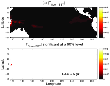
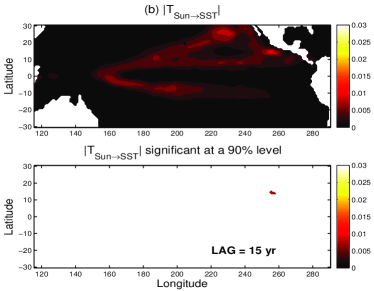
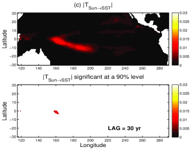
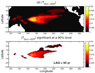
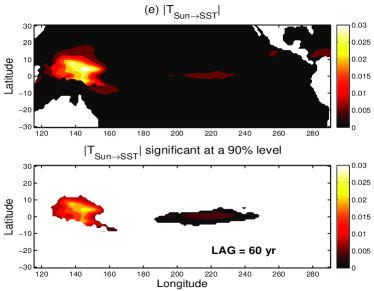
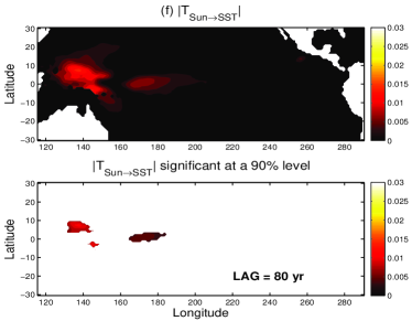
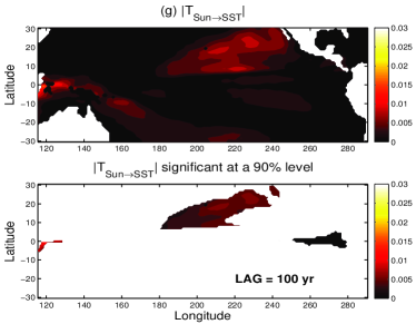
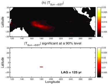
Figure S1: The absolute information flow estimated using the bivariate formula from the delayed series of sunspot numbers (SSN) to those of the sea surface temperature (SST) in the Pacific Ocean (in nats/month). The SST time series between January 1980 - December 2017 are used. In each subplot, the lower panel shows only the value that is significant at a 90% confidence level, and indicated on it is the delay (in years).

We first use the 2D version of Eq. (7) (cf. (8)) to do a rough estimate for the information flow from SSN to the SST at each grid point, given the time series as described in the preceding section. This is the practice how teleconnection patterns are identified using correlation analysis, but here the computed is information flow. (Different from the symmetric correlation, here the information flow in the opposite direction is by computation insignificant, just as expected.) We then form delayed time series for SSN, given time delays $n=1,2,...$, and repeat the above step. For convenience, denote an SSN series with delay $n$ by SSN($-n$). We find that the resulting information flow is not significant at a 90% confidence level, or has a structure bearing no resemblance to the desired pattern, until $n$ approaches 45 years; see Supplementary Figure S1, for a number of examples. Here the data we are using are the SST from 01/1980 through 12/2017 (SST are most reliable after 1979), and the SSN data are correspondingly from 01/1935 through 12/1972. Note that using the time delayed coordinates we can reconstruct a dynamical system which is topologically equivalent to the one that originally generates the time series, thanks to Takens’ embedding theoremTakens1980 . Here, based on the above rough estimates, we choose to form a dynamical system with components corresponding to the SST series and the time-delayed series SSN($-n$) with $n$ ranging from 22-50 years. Note one is advised not to choose two delays too close. SSN is dominated by low-frequency processes; two close series thus-formed may not be independent enough to span a subspace, and hence may lead to singularity. Here we choose SSN series at delays of 22-50 years every 5 years or 60 steps. We have tried many other sampling intervals and found this is the best. This makes sense: An interval of 5 years put the two series approximately at the opposite phases in a solar cycle. From the thus-generated multivariate series, we then compute the information flow from SSN($-45$ years) to the Pacific SST, using formula (7).

A note on the embedding coordinates. In general, it is impossible to reconstruct exactly the original dynamical system from the embedding coordinates; it is just a topologically equivalent one. That also implies that the reconstruction is not unique. Other choices with delayed time series may serve the purpose as well, provided that they are independent of other coordinates; see Abarbanel1996 for empirical methods for time delay choosing. Fortunately, this does not make a problem for our causal inference, thanks to a property of the information flow ab initio, which asserts that

• The information flow between two coordinates of a system stays invariant upon arbitrary nonlinear transformation of the remaining coordinates.

More details are referred to the Method Section. This remarkable property implies that the embedding coordinates do not matter in evaluating the information flow from SSN to SST; what matters is the number of the coordinates, i.e., the dimension, of the system, which makes a topological invariant. There exist empirical ways to determine the dimension of a system, e.g., those as shown in Abarbanel1996 . Here we choose by adding new coordinates and examining the information flow; if it does not change any more, the process stops and the dimension is hence determined. For this problem, as shown above, the SSN series at delays of 22-50 years every 5 years are chosen. This results in 6 auxiliary coordinates, which together with the SST and SSN(-45 years) series make a system of dimension 8.

The spatial distribution of the absolute information flow, or “causal structure” as will be referred to henceforth, from SSN($-45$ years) to the Pacific SST is shown in Fig. 1.

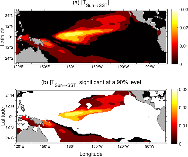
Figure 1: (a) The absolute information flow from the delayed (by 45 years) series of sunspot numbers to those of the sea surface temperature in the Pacific Ocean (in nats/month). The pattern resembles very much the El Niño Modoki mode as shown in the Fig. 2b of Ashok et al. (2007)Ashok2007 . Here information flow means the transfer of predictability from one series to another. It is computed with Eq. (7) in section 2. (b) As (a), but only the information flow significant at a 90% confidence level is shown.

Remarkably, the causal structure in Fig. 1a is very similar to the El Niño Modoki pattern, as given by, say, Ashok et al.Ashok2007 . (Please see their Fig. 2b.) That is to say, the information flow from SSN to the Pacific SST does form a spatially coherent structure resembling to El Niño Modoki. The computed information flow is significant at a 90% confidence level, as shown in Fig. 1b.

Comparing to the rough estimate in the bivariate case (see Supplementary Figure S1d), Fig. 1a has a horseshoe structure pronounced in the upper part, plus a weak branch in the Southern Hemisphere. This is just as the El Niño Modoki structure as obtained by Ashok et al.Ashok2007 (see their Fig. 2b). This indicates that the bivariate information flow analysis provides a good initial guess, but the result is yet to be rectified due to the incorrect dimensionality.

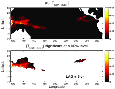
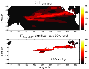
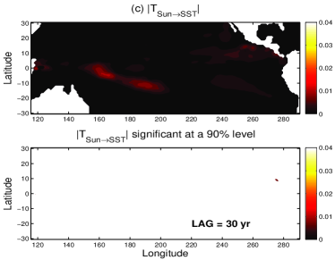
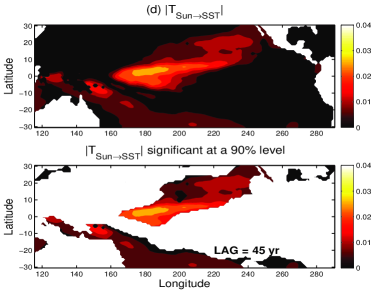
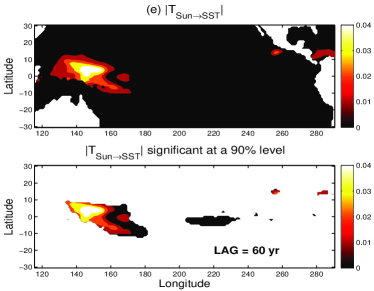
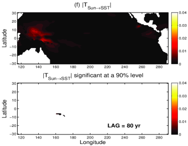
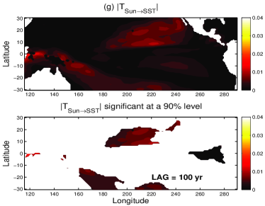
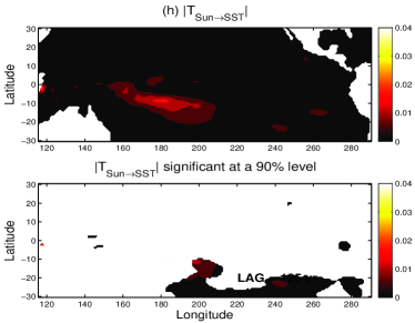
Figure S2: As Supplementary Figure S1, but the information flows are estimated using the multivariate formula, with the embedding coordinates formed with SSN series lagged by 22-50 years every 5 years.

The information flows with other time delays have also been computed. Shown in Supplementary Figure S2, are a number of examples. As can be seen, except those around 45 years (about 44-46 years, to be precise), other delays either yield insignificant information flows or do not result in the desired causal pattern.

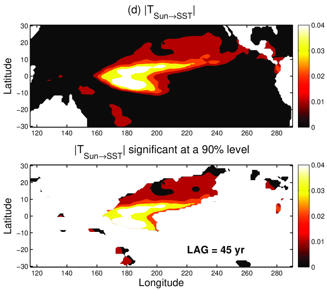
Figure S3: The absolute information flow from the SSN series delayed by 45 years to those of the SST in the Pacific Ocean (in nats/month). It is estimated with the multivariate formula using embedding coordinates formed with SSN series delayed by 22-50 years every 5 years. The SST time series between January 1980 - December 2005 are used. In each subplot, the lower panel shows only the value that is siginificant at a 90% confidence level.

Since we are about to predict, it is desirable to perform the causality analysis in a forecast fashion, i.e., to pretend that the EMI over the forecast period be unavailable. We have computed the information flow with different years of availability. Shown in Fig. S3 is the information flow as that in Fig. 1, but with SST data available until the year of 2005. Obviously, the causal pattern is still there and significant, and, remarkably, it appears even more enhanced, probably due to the frequent occurrences of the event during that period.

As information flow tells the transfer of predictability, SSN forms a natural predictor for El Niño Modoki. This will be further confirmed in the next section.

Projection of El Niño Modoki. The remarkable causal pattern in Fig. 1 implies that it may be possible to make projections of El Niño Modoki many years ahead of time. Based on it we hence conjecture that the lagged SSN series be the desired covariate. Of course, due to the short observation period, the data needed for parametric estimation are rather limited– This is always a problem for climate projection.

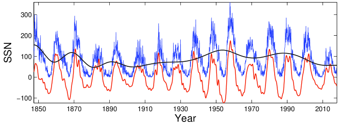
Figure S4: The original monthly SSN series (blue), lowpass-filtered series (black), and bandpass-filtered series (red).

Let us start with a simple linear regression model for the prediction of El Niño Modoki Index (EMI) from SSN. Build the model using the EMI data from 1975-2005 ($30\times 12=600$ equations), leaving the remaining years after 2005 for prediction. For each EMI, the model inputs are the SSNs at lead times of 50 years through 22 years (336 in total), guided by the causality analysis in the preceding section. For best result, the annual signals and the signals longer than 11 years are filtered from the SSN series. The filtering is fulfilled through wavelet analysis with the orthonormal spline wavelets built in LA2007 . Since it is required that the series length be a power of 2, we choose a time range for the monthly SSN series from May 1847 to December 2017, depending on the availability of the data when this research was initialized. This totals 170 years and 8 months (170.67 years), or $2^{11}=2048$ time steps. The upper bound scale level for the wavelet analysis is set $8$, which gives a lower period of $2^{-8}\times 170.67=0.67$ years; the lower bound scale level is chosen to be 4, resulting an upper period of $2^{-4}\times 170.67=10.67$ years. In doing this the seasonal cycle and the interdecadal variabilities are effectively removed (Supplementary Figure S4). With the pretreated SSN series the prediction is launched, and the result is shown in Fig. 2a.

We would not say that the projection in Fig. 2a with such a simple linear model is successful, but the 2015/2016 event is clearly seen. The strong 2009 event is not correct; it has a phase error. The general trend between 2005-2018 seems to be fine. Beyond 2018 it becomes off the mark.

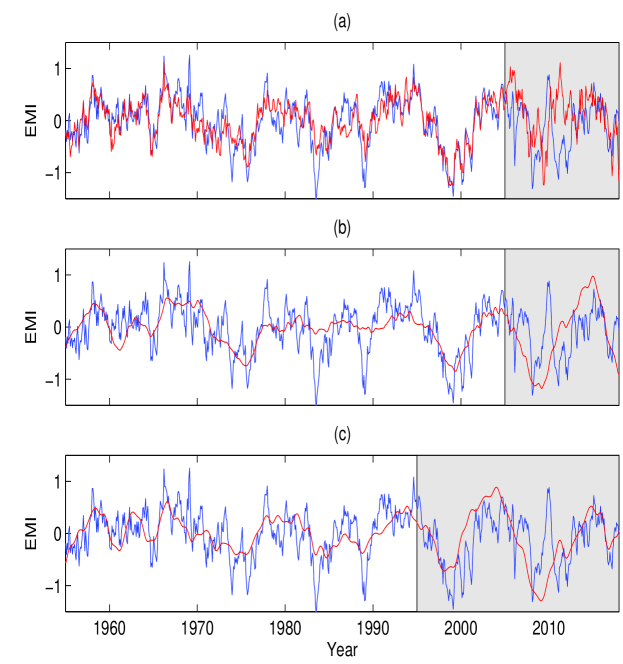
Figure 2: Projection of the El Niño Modoki index based solely on the sunspot numbers 22-50 years ago with a simple linear regression model. (a) The SSN series is bandpass filtered with the annual signals and the signals longer than 11 years removed. (b) Only 25 first principal components are used as inputs. (c) The SSN series is bandpass filtered as in (a), and only the 25 first principal components are used as inputs. The shaded period is for prediction (note in (c) the period for prediction is 1995-), and the predicted index is in red.

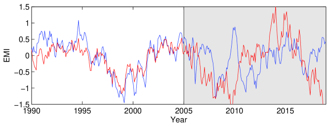
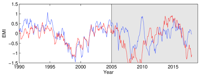
Figure S5: Projection of the El Niño Modoki Index (EMI) based solely on the SSN 22-50 years ago with a simple linear regression model. Upper: The SSN series as input is not filtered. Lower: The SSN series is low-pass filtered. The observed EMI is in blue, while the projected is in red.

It would be of some use to see how the simple linear prediction may depend on some factors, though it cannot be said successful and hence a quantitative investigation does not make sense. We hope to learn some experience for the machine learning to be performed soon. First, we check the effect of filtering. As shown in Supplementary Figure S5, without filtering, the result is much noisy, the 2015/2016 event is too strong, and the strong 2009/2010 event completely disappears; with low-pass filtering (only the signals below a year are filtered), the result is similar, only with the noise reduced and the 2015/2016 event better.

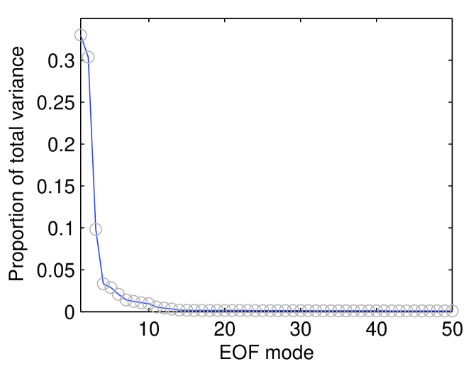
Figure S6: NormaliEd variance vs. EOF mode. The EOF analysis is performed with the SSN time series with delays from 22-50 years, which form a vector with 336 members of series.

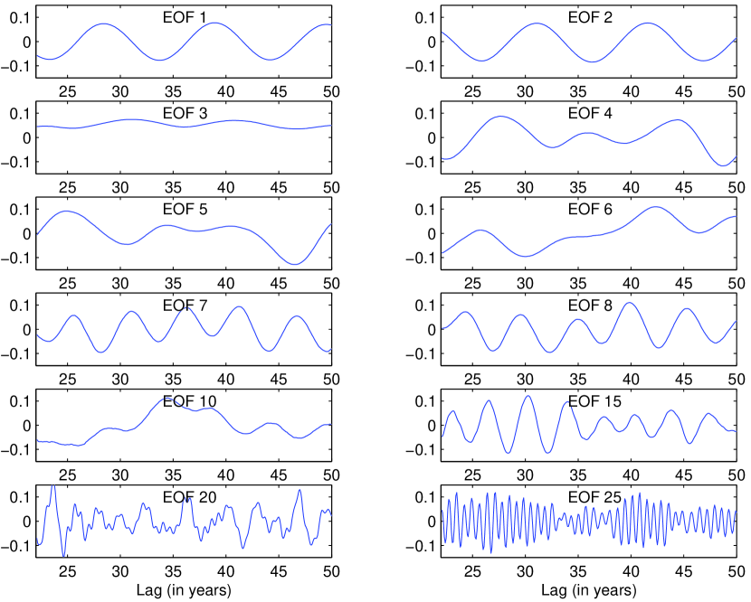
Figure S7: Examples of the EOF modes as described in Supplementary Figure S6.

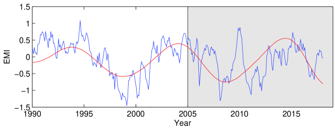
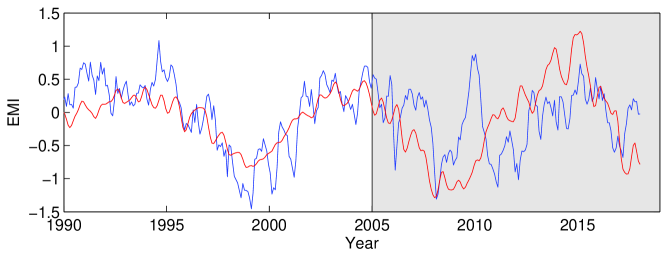
Figure S8: As Figure 2b, but the projection uses, respectively, the first 8 and 50 principal components as inputs.

Second, we perform an empirical orthogonal function (EOF) analysis for the 336 time-delayed SSN series, which forms a column vector with 336 entries at each time step: [${\rm SSN}(n-600),{\rm SSN}(n-599),...,{\rm SSN}(n-265)$]^T. The variance for each EOF mode is plotted in Supplementary Figure S6. From it the first 8, 25, and 50 principal components (PCs) approximately account for 84%, 89%, and 92% of the total variances, respectively. Some examples of the EOF modes are plotted in Supplementary Figure S7. Now use the first 25 PCs as inputs and repeat the above process to make the projection. The result is shown in Fig. 2b. Obviously, during the 12 years of prediction from 2005 to 2017, except for the strong 2009/2010 event, the others are generally fine. Projections with other numbers of PCs have also been conducted. Shown in Supplementary Figure S8 are examples with 8 and 50 PCs, respectively. It is particularly interesting to see that, except for the 2009/2010 event, the case with 8 PCs already captures the major trend of the EMI evolution. Recall that, in performing the information flow analysis, we have found that the reconstructed dynamical system approximately has a dimension of 8. Here the prediction agrees with the dimension inference.

Because of the encouraging linear model result, it is desirable to achieve a better projection using more sophisticated tools in deep learning, e.g., the back propagation (BP) neural network algorithmGoodfellow2016 . (At the preparation of the original version of this manuscript, we noticed that recently there have been applications of other machine learning methods to El Niño forecasts, e.g., Ham2019 .) Three hidden layers are used for the BP neural network forecast. Again, a major issue here is the short observational period which may prevent from an appropriate training with many weights. We hence use only 8, 6, and 1 neurons for the first, second, and third hidden layers, respectively, as schematized in Fig. 3. This architecture will be justified soon. To predict an EMI at step (month) $n$, written $y$, a $336\times 1$ vector ${\bf x}$ is formed with SSN data at steps (months) $n-600,n-599,...,n-265$, the same as the case with lead times of 50-22 years for the above simple linear regression model. But even with the modest number of parameters, the data are still not enough. To maximize the use of the very limited data, we choose the first 25 principal components (PCs) that account for 90% of the total variance. We hence train the model with these 25 inputs (rather than 336 inputs); that is to say, ${\bf x}$ now is a $25\times 1$ vector, which greatly reduces the number of parameters to train. (See below in Eq. (1): The ${\bf w}_{1}$ is reduced from a $8\times 336$ matrix to a $8\times 25$ matrix.) Once this is done, ${\bf x}$ is input into the following equation to arrive at the prediction of $y$:

$$y={{\bf w}_{4}}\ {\rm tansig}({{\bf w}_{3}}\ {\rm tansig}({\bf w}_{2}\ {\rm tansig}({\bf w}_{1}\ {\bf x}+{\bf b}_{1})+{\bf b}_{2})+{\bf b}_{3})+{\bf b}_{4},$$ (1)

where the matrices/vectors of parameters ${\bf w}_{1}$ ($8\times 25$ matrix), ${\bf w}_{2}$ ($6\times 8$ matrix), ${\bf w}_{3}$ ($1\times 6$ row vector), ${\bf w}_{4}$ ($1\times 1$ matrix—a scalar), ${\bf b}_{1}$ ($8\times 1$ vector), ${\bf b}_{2}$ ($6\times 1$ vector), $b_{3}$ (scalar) and $b_{4}$ (scalar) are obtained through training. An illustrative explanation is seen in Fig. 3. As has been argued (e.g. Heaton2008 ) that the number of hidden neurons should be kept fewer than 2/3 the size of the input and output layers, i.e., $\frac{2}{3}\times(25+1)=17$ here. With this architecture we have 15 neurons in total, meeting the requirement.

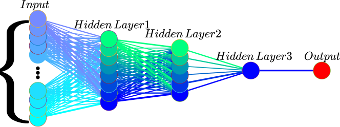
Figure 3: The neural network architecture used in this study, which is made of an input layer, an output layer, and three hidden layers. The symbols are the same as those in (1). The matrices/vectors ${\bf w}_{i}$ and ${\bf b}_{i}$ ($i=1,2,3,4$) are obtained through training. To predict the El Niño Modoki Index (EMI) at month/step $n$, ${\rm EMI}(n)$, find the first 25 principal components of [${\rm SSN}(n-600),{\rm SSN}(n-599),...,{\rm SSN}(n-265)$]^T, a column vector with 336 entries, and form the input vector ${\bf x}$. The final output $y$ is the predicted ${\rm EMI}(n)$. Iterating on $n$, we can get a prediction of EMI for any target time interval.

To predict the EMI at month/step $n$, ${\rm EMI}(n)$, organize ${\rm SSN}(n-600),{\rm SSN}(n-599),...,{\rm SSN}(n-265)$, that is, the SSNs lagged by 50 through 22 years, into a $336\times 1$ vector. Project it onto the first 25 EOFs as obtained above, and obtain ${\bf x}$, a vector with 25 entries. Input ${\bf x}$ into Eq. (1). The final output $y$ is the predicted ${\rm EMI}(n)$. Iterating on $n$, we can get a prediction of EMI for any target time interval.

The 5-year data prior to the starting step of prediction are used for validation. In this study, we start off predicting EMI at January 2008. We hence take the data over the period from January 2003 through December 2007 to form the validation set, and the data until December 2002 to train the model. 10,000 runs have been performed, and we pick the one that minimizes the mean square error (MSE) over the validation set. This is plotted in Fig. 4. Remarkably, the 12-year long index has been forecast with high skill (corr. coeff.=0.91). Particularly, the strong 2009/10 event is well predicted, so is the 2019/20 event. The 2014/16 event, which has made the El Niño forecasts off the mark in 2014-15, appears a little weaker but also looks fine by trend.

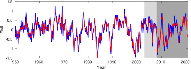
Figure 4: Projection of the El Niño Modoki index based solely on the sunspot numbers 22-50 years ago with the back propagation neural network algorithm. The EMI is in blue, while the predicted index is in red. Lightly shaded is the period over which the validation set is formed, and the period with dark shading is for prediction.

Out of the 10,000 runs we select the top 10% with lowest MSE over the validation set (January 2003-December 2007) to form an ensemble of predictions for the 12 years of EMI (January 2008 till now). The spread, the mean, and the standard deviation of the ensemble are shown in Fig. 5. Also overlaid is the observed EMI (blue). As can be seen, the uncertainty is rather limited for a climate projection.

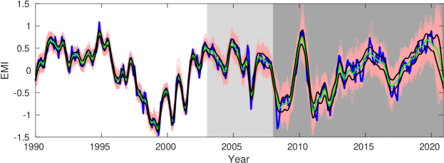
Figure 5: The 1000 predictions showing the spread of the ensemble. Overlaid are the observed EMI (blue), the mean of the realizations (cyan), and the mean plus and minus the standard deviation (black). The light shading marks the period for validation, while the darker shading marks the prediction period.

We have examined how the projection performance may vary with the choices of PCs, the number of neurons, and the lags. The PCs of a vector are obtained by projecting it onto the EOF modes (described above), which possess variances and structures as plotted in Supplementary Figures S6 and S7, respectively. Shown in Fig. 6 is the MSE as a function of the number of PCs. Obviously with 25 PCs the MSE is optimized, and that is what we have chosen for the network architecture. But if one takes a closer look, the MSE does not decrease much beyond 8. Recall that, in performing the causality analysis, we have seen that the reconstructed dynamical system approximately has a dimension 8. Fig. 6 hence provides a verification of the dimension inference.

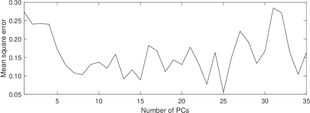
Figure 6: Mean square error for the neural network prediction as a function of number of principal components.

The EOF modes associated with these 8 PCs are plotted in Supplementary Figure S7. As can be seen, except for the 11-year process, among others, the 5-year variability is essential. This is, again, consistent with what we have done in forming the embedding coordinates: select the delayed series every 5 years.

The dependence of the model performance on the number of neurons has also been investigated. We choose 1 neuron for layer 3, leaving the numbers of layers 1 and 2 for tuning. The result is contoured in Fig. 7. As can be clearly seen, a minimum of MSE appears at (8,6), i.e., when the numbers of hidden layer 1 and layer 2 are, respectively, 8 and 6. This is what we have chosen to launch the standard prediction.

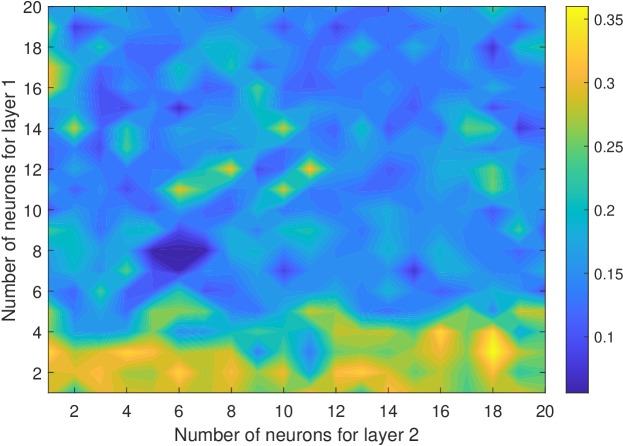
Figure 7: Mean square error as function of number of neurons.

Also studied is the influence of the lags for the delayed series. In Fig. 8 the MSE is shown as function of the lower and upper bounds of the delays (in years). From the figure there are a variety of local minima, but the one at (22, 50) is the smallest one. That is to say, the series with delays from 22 to 50 years make the optimal embedding coordinates, and this is just we are choosing.

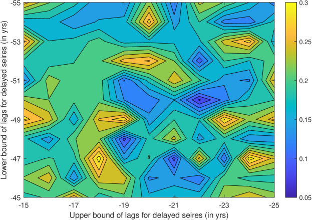
Figure 8: Mean square error as function of lags.

It is known that machine learning suffers from the problem of reproducibilityHutson2018 . But in this study, as we have shown above, the prediction guided by the information flow analysis is fairly robust, with uncertainty acceptably small for climate projection. For all that account, at least the El Niño Modoki events so far are mostly predictable at a lead time of more than 10 years.

Concluding remarks. The rigorously developed theory of information flow in terms of predictability/uncertainty transfer provides a natural way for one to seek for predictor(s) for a dynamical phenomenon. In this study, it is found that the delayed causal pattern from SSN to the Pacific SST resembles very much the El Niño Modoki mode; the former hence can be used to predict the latter. Indeed, as detailed above, with all the observations we have had so far, El Niño Modoki can be essentially predicted based solely on SSN at a lead time of 12 years or over. Particularly, the strong event in 2009/10 and the elusive event during 2014-16 have been well predicted (Fig. 2b).

We, however, do NOT claim that El Niño Modoki is ultimately driven by solar activities. It is NOT our intention in this study to investigate on the dynamical aspects of this climate mode. We just present an observational fact on fulfilled predictions. There is still a very long way to go in unraveling the dynamical origin(s) of El Niño Modoki. The success of atmosphere-ocean coupled models during the past decades confirms that the canonical El Niño is an intrinsic mode in the climate system; El Niño Modoki may be so also. Nonetheless, despite the long-standing controversy on the role of solar activity in climate change (see a review in Bard2006 ), there does exist evidence on the lagged response as identified here; the North Atlantic climate response is such an exampleScaife2013 .

As a final remark, it is interesting to see that the maximum information flow from the SSN lagged by 45 years to the Pacific SST agrees very well with frequent occurrences of El Niño Modoki during the period of 2000-2010: three of the four El Niño events are of this type (i.e., the 02/03, 04/05, 09/10 episodes). If we go back to 45 years ago, the sun is most active during the period of 1955-1965 (Fig. 9) Particularly, in the wavelet spectrum, there is a distinct high at the scale level of 4 (corresponding to a time scale of $2^{-4-(-15)}=2048$ days $\approx 5.6$ years)—Recall that this is roughly the sampling interval we used in choosing the time-delay series to form the ${\nu}$-dimensional system and compute the information flow. After that period, the sun becomes quiet, correspondingly we do not see much El Niño Modoki for the decade 2010-20. But two peaks of SSN are seen in the twenty years since 1975-78. Does this correspondence herald that, after entering 2020, in the following two decades, El Niño Modoki may frequent the equatorial Pacific again? We don’t know whether this indeed points to a link, but when this project was initiated early in 2018, the projected El Niño Modoki and La Niña Modoki already occurred recently. This question, among others, are to be addressed in future studies. (For reference, the codes used in this study are available at
http://www.ncoads.org/enso_modoki_data_codes.tar.gz. )

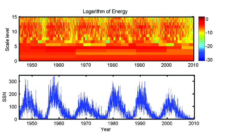
Figure 9: Daily series and orthonormal wavelet spectrum of the sunspot numbers based on the spline wavelets built in LA2007 .

METHOD

Estimation of information flow and causality among multivariate time series. Information flow is a fundamental notion in general physics which has applications in a wide variety of scientific disciplines (see Liang2016 and references therein). Its importance lies beyond the literal meaning in that it implies causation, uncertainty propagation, predictability transfer, etc. Though with a history of research for more than 30 years, it has just been put on a rigorous footing and derived from first principles, initially motivated by the predictability study in atmosphere-ocean scienceLK2005 . Since its birth it has been validated with many benchmark dynamical systems such as baker transformation, Hénon map, Rössler system, etc. (cf. Liang2016 Liang2014 ), and has been applied with success to different problems in earth system science, neuroscience and quantitative finance, e.g., Vannitsem2019 , Dionisis2019 , Stips2016 , to name a few. Hereafter we just give a very brief introduction.

Consider a dynamical system

$$\frac{d{\bf x}}{dt}={\bf F}(t;{\bf x})+{\bf B}(t;{\bf x})\dot{{\bf w}},$$ (2)

where ${\bf x}$ and ${\bf F}$ are ${\nu}$-dimensional vector, ${\bf B}$ is a ${\nu}$-by-$m$ matrix, and $\dot{{\bf w}}$ an $m$-vector of white noise. Here we follow the convention in physics and do not distinguish the notation of a random variable from that of a deterministic variable. Liang (2016)Liang2016 established that the rate of uncertainty (in terms of Shannon entropy) transferred from $x_{2}$ to $x_{1}$, or rate of information flowing from $x_{2}$ to $x_{1}$ (in nats per unit time), is:

$$T_{2\to 1}=-E\left[\frac{1}{\rho_{1}}\int_{{}^{{\nu}-2}}\frac{\partial(F_{1}\rho_{{\backslash 2}})}{\partial x_{1}}dx_{3}...dx_{\nu}\right]+\frac{1}{2}E\left[\frac{1}{\rho_{1}}\int_{R^{{\nu}-2}}\frac{\partial^{2}(g_{11}\rho_{{\backslash 2}})}{\partial x_{1}^{2}}dx_{3}...dx_{\nu}\right],$$ (3)

where $E$ stands for mathematical expectation, $\rho_{1}=\rho_{1}(x_{1})$ is the marginal probability density function (pdf) of $x_{1}$, $\rho_{{\backslash 2}}=\int\rho dx_{2}$, and $g_{11}=\sum_{j=1}^{m}b_{1j}b_{1j}$. The units are in nats per unit time. Ideally if $T_{2\to 1}=0$, then $x_{2}$ is not causal to $x_{1}$; otherwise it is causal (for either positive or negative information flow). But in practice significance test is needed.

Generally $T_{2\to 1}$ depends on $(x_{3},...,x_{\nu})$ as well as $(x_{1},x_{2})$. But it has been established thatLiang2018 it is invariant upon arbitrary nonlinear transformation of $(x_{3},x_{4},...,x_{\nu})$, indicating that information flow is an intrinsic physical property. Also established is the principle of nil causality, which asserts that, if the evolution of $x_{1}$ is independent of $x_{2}$, then $T_{2\to 1}=0$. This is a quantitative fact that all causality analyses try to verify in applications, while in the framework of information flow it is a proven theorem.

In the case of linear systems where ${\bf F}({\bf x},t)={\bf A}{\bf x}$, ${\bf A}=(a_{ij})$, the formula (3) becomes quite simpleLiang2016 :

$$T_{2\to 1}=a_{12}\frac{\sigma_{12}}{\sigma_{11}},$$ (4)

where $\sigma_{ij}$ is the population covariance. An immediate corollary is that causation implies correlation, while correlation does not imply causation, fixing the long-standing philosophical debate over causation versus correlation ever since Berkeley (1710)Berkeley1710 .

To arrive at a practically applicable formula, we need to estimate (4), given ${\nu}$ time series. The estimation roughly follows that of Liang (2014)Liang2014 , and can be found in Liang2021 . The following is just a brief summary of some relevant pieces as detailed in Liang2021 .

Suppose we have ${\nu}$ time series, $x_{i}$, $i=1,...,{\nu}$, and these series are equi-spaced, all having $N$ data points $x_{i}(n)$, $n=1,2,...,N$. Assume a linear model ${\bf F}({\bf x};t)={\bf A}{\bf x}$, ${\bf A}=(a_{ij})$ being a ${\nu}\times{\nu}$ matrix), and ${\bf B}$ being a ${\nu}\times{\nu}$ diagonal matrix. To estimate $T_{2\to 1}$, we first need to estimate $a_{12}$. As shown before in Liang2014 , when $a_{ij}$ and $b_{i}$ are constant, the maximal likelihood estimator (mle) is precisely the least square solution of the following $N$ (overdetermined) algebraic equations

$$\sum_{j=1}^{\nu}a_{1j}x_{j}(n)=\dot{x}_{1}(n),\qquad\qquad n=1,...,N$$ (5)

where $\dot{x}_{1}(n)=(x_{1}(n+1)-x_{1}(n))/\Delta t$ is the differencing approximation of $dx_{1}/dt$ using the Euler forward scheme, and $\Delta t$ is the time stepsize (not essential; only affect the units). Following the procedure in Liang2014 , the least square solution of $(a_{11},...,a_{1{\nu}})$, $(\hat{a}_{11},...,\hat{a}_{1{\nu}})$, satisfies the algebraic equation

$$\left[\begin{array}[]{ccc}C_{1,1}&...&C_{1,{\nu}}\\ \vdots&\vdots&\vdots\\ C_{{\nu},1}&...&C_{{\nu},{\nu}}\end{array}\right]\left[\begin{array}[]{c}\hat{a}_{11}\\ \vdots\\ \hat{a}_{1{\nu}}\end{array}\right]=\left[\begin{array}[]{c}C_{1,d1}\\ \vdots\\ C_{{\nu},d1}\end{array}\right],$$

where

$$C_{ij}=\frac{1}{N}\sum_{n=1}^{N}(x_{i}(n)-\bar{x}_{i})(x_{j}(n)-\bar{x}_{j})$$

$$C_{i,dj}=\frac{1}{N}\sum_{n=1}^{N}(x_{i}(n)-\bar{x}_{i})(\dot{x}_{j}(n)-{\bar{\dot{x}}}_{j})$$

are the sample covariances. Hence $\hat{a}_{12}=\frac{1}{\det{\bf C}}\cdot\sum_{j=1}^{\nu}\Delta_{2j}C_{j,d1}$ where $\Delta_{ij}$ are the cofactors. This yields an estimator of the information flow from $x_{2}$ to $x_{1}$:

$$\hat{T}_{2\to 1}=\frac{1}{\det{\bf C}}\cdot\sum_{j=1}^{\nu}\Delta_{2j}C_{j,d1}\cdot\frac{C_{12}}{C_{11}},$$ (7)

i.e., Eq. (7) in section 2. Here $\det{\bf C}$ is the determinant of the covariance matrix ${\bf C}$, and now $T$ is understood as the MLE of $T$. We slightly abuse notation for the sake of simplicity.) For two-dimensional (2D) systems, ${\nu}=2$, the equation reduces to

$$\hat{T}_{2\to 1}=\frac{C_{11}C_{12}C_{2,d1}-C_{12}^{2}C_{1,d1}}{C_{11}^{2}C_{22}-C_{11}C_{12}^{2}},$$ (8)

recovering the familiar one as obtained in Liang2014 and frequently used in applications (e.g., Stips2016 , Vannitsem2019 , Dionisis2019 ).

The significance of $\hat{T}_{2\to 1}$ of (7) can be tested following the same strategy as that used in Liang2014 . By the MLE property (cf. Garthwaite1995 , when $N$ is large, $\hat{T}_{2\to 1}$ approximately follows a Gaussian around its true value with a variance $\left(\frac{C_{12}}{C_{11}}\right)^{2}{\hat{\sigma}}_{a_{12}}^{2}$. Here ${\hat{\sigma}}_{a_{12}}^{2}$ is the variance of $\hat{a}_{12}$, which is estimated as follows. Denote by ${\bm{\theta}}$ the vector of parameters to be estimated; here it is $(a_{11},a_{12},a_{13},...,a_{1{\nu}};b_{1})$. Compute the Fisher information matrix ${\bf I}=(I_{ij})$

$$I_{ij}=-\frac{1}{N}\sum_{n=1}^{N}\frac{\partial^{2}\log\rho({\bf x}_{n+1}|{\bf x}_{n};\hat{{\bm{\theta}}})}{\partial\theta_{i}\partial\theta_{j}}$$

where $\rho({\bf x}_{n+1}|{\bf x}_{n})$ is a Gaussian for a linear model:

$$\rho({\bf x}_{n+1}|{\bf x}_{n}) =\frac{1}{[(2\pi)^{2}\det({\bf B}{\bf B}^{T}\Delta t)]^{1/2}}$$

$$\qquad\times e^{-\frac{1}{2}({\bf x}_{n+1}-{\bf x}_{n}-{\bf A}{\bf x}_{n}\Delta t)^{T}({\bf B}{\bf B}^{T}\Delta t)^{-1}({\bf x}_{n+1}-{\bf x}_{n}-{\bf A}{\bf x}_{n}\Delta t)}.$$

The computed entries are then evaluated using the estimated parameters, and hence the Fisher information matrix is obtained. It has been established (cf. Garthwaite1995 ) that ${\bf I}^{-1}/N$ is the covariance matrix of $\hat{{\bm{\theta}}}$, from which it is easy to find the entry $\hat{\sigma}_{a_{12}}^{2}$ [here it is the entry (2,2)]. Given a level, the significance of an estimated information flow can be tested henceforth.

Data availability

The data used in this study include the SST and sunspot number (SSN) from National Oceanic and Atmospheric Administration (NOAA) (SST: http://www.esrl.noaa.gov/psd/data/gridded/cobe2.html; SSN: https://wwww.esrl.noaa.gov/psd/gcos_wgsp/Timeseries/Data/sunspot.long.data), and the El Niño Modoki Index (EMI) from Japan Agency for Marine-Earth Science and Technology (JAMSTEC) (http://www.jamstec.go.jp/aplinfo/sintexf/e/elnmodoki/data.html). Among them SST has a horizontal resolution of $1^{\rm o}\times 1^{\rm o}$. Temporally all of them are monthly data, and at the time when this study was initiated, SST, EMI, and SSN respectively have a time coverage of 01/1850-12/2018, 01/1870-11/2018, and 05/1847-12/2017. Daily SSN is also used for spectral analysis; it covers the period 15/04/1921-31/12/2010.

Code availability

All the codes (and some of the downloaded data) are available at
http://www.ncoads.org/upload/enso_modoki_data_codes.tar.gz

Acknowledgments. The long discussion with Richard Lindzen on August 17, 2019, and the email exchange later on in late February 2020 are sincerely appreciated. The comments from Dmitry Smirnov and four anonymous reviewers have helped improve the manuscript. We thank NOAA and JAMSTEC for making the data available, and the NUIST High Performance Computing Center for providing computational resources. This study is partially funded by National Science Foundation of China (No. 41975064), and the 2015 Jiangsu Program for Innovation Research and Entrepreneurship Groups.

Author contributions. XSL: idea, methodology, experiment design, computation (causality analysis and prediction), writing; FX: experiment design, computation (causality analysis); YR: experiment design, computation (prediction). All authors discussed the study results.

Competing interests. The authors declare no competing interests.

El Niño Modoki thus far can be mostly predicted more than 10 years ahead of time

X. San Liang,  Fen Xu,  & Yineng Rong

Supplementary Information

References

- (1) McPhaden, M.J. (2015), Playing hide and seek with El Niño, Nature Climate Change 5, 791-795.
- (2) Ashok, K., and T. Yamagata (2009), The El Niño with a difference. Nature 461, 481.
- (3) Trenberth, K.E., and D.P. Stepaniak (2001), Indices of El Niño evolution. J. Clim. 14, 1697-1701.
- (4) Larkin, N.K., and D.E. Harrison (2005), Global seasonal temperature and precipitation anomalies during El Niño autumn and winter. Geophys. Res. Lett. 32, L16705.
- (5) Yu, J.Y., and H.Y. Kao (2007), Decadal changes of ENSO persistence barrier in SST and ocean heat content indices: 1958-2001. J. Geophys. Res. Atmos. D13106b.
- (6) Lee, T., and M.J. McPhaden (2010), Increasing intensity of El Niño in the central equatorial Pacific. Geophys. Res. Lett. 37, L14603.
- (7) Yu, J.Y., and S.T. Kim (2010), Three evolution patterns of central-pacific El Niño . Geophys. Res. Lett. 37, L08706.
- (8) Ashok, K., S.K. Behera, S.A. Rao, H.Y. Weng, and T. Yamagata (2007), El Niño Modoki and its possible teleconnection. J. Geophys. Res. Oceans 112, C11007.
- (9) Kug, J.S., F.F. Jin, and S.I. An (2009), Two types of El Niño events: cold tongue El Niño and warm pool El Niño . J. Clim. 22, 1499-1515.
- (10) Fu, C., H.F. Diaz, and J.O. Fletcher (1986), Characteristics of the response of sea surface temperature in the central Pacific associated with warm episodes of the Southern Oscillation. Mon. Weath. Rev. 114, 1716-1738.
- (11) Wang, C.Z., C. Deser, J.Y. Yu, P. Dinezio, and A. Clement (2017), “El Niño and Southern Oscillation (ENSO): A Review” in Coral Reefs of the Eastern Tropical Pacific, P.W. Glynn et al., Eds., Springer, Netherlands, pp. 85-106.
- (12) Behera, S., and T. Yamagata (2018), Climate Dynamics of ENSO Modoki Phenomena, Oxford Research Encyclopedias.
- (13) Mo, K.C. (2010), Interdecadal modulation of the impact of ENSO on precipitation and temperature over the United States. J. Clim. 23, 3639-3656.
- (14) Barnston, A.G., A. Kumar, L. Goddard, and M.P. Hoerling (2005), Improving seasonal prediction practices through attribution of climate variability. Bull. Amer. Meteorol. Soc. 2005, 59-72.
- (15) Xie, R., and F.-F. Jin (2018), Two leading ENSO modes and El Niño Types in the Zebiak-Cane Model. J. Clim. 31, 1943-1962.
- (16) Zebiak, S.E., and M.A. Cane (1987), A model El Niño-Southern Oscillation. Mon. Weath. Rev. 115, 2262-2278.
- (17) Chen, D., and Coauthors (2015), Strong influence of westerly wind bursts on El Niño diversity. Nature Geoscience DOI:10.1038/NGEO2399.
- (18) Tang, Y.M., and Coauthous (2018), Progress in ENSO prediction and predictability study. National Science Review 5, 826-839.
- (19) Von Storch, H. (2001), “Statistics — an indispensable tool in dynamical modeling” in Models in Environmental Research, H. von Storch and G. Flöser, Eds., Springer Verlag.
- (20) Liang, X.S., and R. Kleeman (2005), Information transfer between dynamical system components. Phys. Rev. Lett. 95, 244101.
- (21) Liang, X.S. (2014), Unraveling the cause-effect relation between time series. Phys. Rev. E. 90, 052150.
- (22) Liang, X.S. (2016), Information flow and causality as rigorous notions ab initio. Phys. Rev. E 94, 052201.
- (23) Liang, X. S. (2018), Causation and information flow with respect to relative entropy. Chaos, 28, 075311.
- (24) Vannitsem, S., Q. Dalaiden, and H. Goose (2019), Testing for dynamical dependence — Application to the surface mass balance over Antarctica. Geophys. Res. Lett. DOI: 10.1029/2019GL084329.
- (25) Hristopulos, D.T., A. Babul, S.A. Babul, L.R. Brucar, and N. Virji-Babul (2019), Disrupted information flow in resting-state in adolescents with sports related concussion. Frontiers in Human Neuroscience 13, 419. DOI: 10.3389/fnhum.2019.00419.
- (26) Stips, A., D. Macias, C. Coughlan, E. Garcia-Gorriz, and X.S. Liang (2016), On the causal structure between CO2 and global temperature. Scientific Reports 6: 21691. DOI: 10.1038/srep21691.
- (27) Johnson, E.N., and S.K. Kannan (2005), Adaptive trajectory control for autonomous helicopters. Journal of Guidance, Control, and Dynamics 28(3), 524-538.
- (28) Kim, P., J. Rogers, J. Sun, and E. Bollt (2017), Causation entropy identifies sparsity structure for parameter estimation of dynamic systems. Journal of Computational and Nonlinear Dynamics 12(1).
- (29) Wallace, J.M., and D.S. Gutzler (1981), Teleconnections in the geopotential height field during the northern hemisphere winter. Mon. Wea. Rev. 109, 784-812.
- (30) Takens, F. (1981), “Detecting strange attractors in turbulence” in Dynamical Systems and Turbulence, Lecture Notes in Mathematics, D.A. Rand, L.-S. Young, Eds., Springer-Verlag, New York, NY, vol. 898, pp. 366-381.
- (31) Abarbanel, H.D.I. (1996), Analysis of Observed Chaotic Data, Springer-Verlag, New York.
- (32) Liang, X.S., and D.G.M. Anderson (2007), Multiscale window transform. SIAM J. Multiscale Model. Simul. 6, No.2, 437-467.
- (33) Goodfellow, I., Bengio, Y., Courville, A. (2016), Deep Learning. MIT Press.
- (34) Ham, Y.-G., J.-H. Kim, and J.J. Luo (2019), Deep learning for multi-year ENSO forecasts. Nature. DOI:10.1038/s41586-019-1559-7.
- (35) Heaton, J. (2008), Introduction to Neural Networks with Java. Heaton Research Inc., 44p pp.
- (36) Hutson, M. (2018), Artificial intelligence faces reproducibility crisis. Science 359, 725-726.
- (37) Bard, E., and M. Frank (2006), Climate change and solar variability: What’s new under the sun? Earth Planet. Sci. Lett. 248, 1-14.
- (38) Scaife, A.A., S. Ineson, J.R. Knight, L. Gray, K. Kodera, and D.M. Smith (2013), A mechanism for lagged North Atlantic climate response to solar variability. Geophys. Res. Lett. 40, 434-439.
- (39) Berkeley, G. (1710), A Treatise on Principles of Human Knowledge.
- (40) Liang, X.S., Normalized multivariate time series causality analysis and causal graph reconstruction. The 37th Conference on Uncertainty in Artificial Intelligence, (submitted).
- (41) Garthwaite, P.H., I.T. Jolliffe, and B. Jones (1995), Statistical Inference. Prentice-Hall, Hertfordshire, UK.