One-shot learning for solution operators of partial differential equations

Abstract

Discovering governing equations of a physical system, represented by partial differential equations (PDEs), from data is a central challenge in a variety of areas of science and engineering. Current methods require either some prior knowledge (e.g., candidate PDE terms) to discover the PDE form, or a large dataset to learn a surrogate model of the PDE solution operator. Here, we propose the first solution operator learning method that only needs one PDE solution, i.e., one-shot learning. We first decompose the entire computational domain into small domains, where we learn a local solution operator, and then we find the coupled solution via either mesh-based fixed-point iteration or meshfree local-solution-operator informed neural networks. We demonstrate the effectiveness of our method on different PDEs, and our method exhibits a strong generalization property.

1 Introduction

Discovering governing equations of a physical system from data is a central challenge in a variety of areas of science and engineering. These governing equations are usually represented by partial differential equations (PDEs). For the first scenario, where we know all the terms of the PDE and only need to infer unknown coefficients from data, many effective methods have been proposed. For example, we can enforce physics-based constraints to train neural networks that learn the underlying physics [1, 2, 3, 4, 5, 6, 7, 8]. In the second scenario, we do not know all the PDE terms, but we have a prior knowledge of all possible candidate terms, several approaches have also developed recently [9, 10, 11].

In a general setup, discovering PDEs only from data without any prior knowledge is much more difficult. To address this challenge, instead of discovering the PDE in an explicit form, in most practical cases, it is sufficient to have a surrogate model of the PDE solution operator that can predict PDE solutions repeatedly for different conditions (e.g., initial conditions). Very recently, several approaches have been developed to learn PDE solution operators by using neural networks such as DeepONet [12, 13, 14] and Fourier neural operator [15, 13]. However, these approaches require large amounts of data to train the networks.

In this work, we propose a novel approach to learn PDE solution operators from only one data point, i.e., one-shot learning. To our knowledge, the use of one-shot learning in this space is very limited. [16] and [17] used few shot learning to learn PDEs and applied it to face recognition. Our method first leverages the locality of PDEs and uses neural networks to learn the system governed by PDEs at a small computational domain. Then for a new PDE condition, we couple all local domains to find the PDE solution. A mesh-based fixed-point iteration (FPI) approach is proposed to learn the PDE solution that satisfies the boundary/initial conditions and local PDE constraints. We also propose two versions of local-solution-operator informed neural networks (LOINNs), which are meshfree, to improve the stability and robustness of finding the solution. Moreover, our one-shot local learning method can extend to multi-dimensional, linear and non-linear PDEs. In this paper, we describe, in detail, the one-shot local learning method and demonstrate on different PDEs for a range of conditions.

2 Methods

We first introduce the problem setup of learning solution operators of PDEs and then present our one-shot learning method.

2.1 Learning solution operators of PDEs

We consider a physical system governed by a PDE defined on a spatio-temporal domain $\Omega\subset\mathbb{R}^{d}$:

$$\mathcal{F}[u(\mathbf{x});f(\mathbf{x})]=0,\quad\mathbf{x}=(x_{1},x_{2},\dots,x_{d})\in\Omega$$

with suitable initial and boundary conditions $\mathcal{B}(u(\mathbf{x}),\mathbf{x})=0$. $u(\mathbf{x})$ is the solution of the PDE and $f(\mathbf{x})$ is a forcing term. The solution $u$ depends on $f$, and thus we define the solution operator as $\mathcal{G}:f(\mathbf{x})\mapsto u(\mathbf{x})$. For nonlinear PDEs, $\mathcal{G}$ is a nonlinear operator.

In many problems, the PDE of a physical system is unknown or computationally expensive to solve, and instead, sparse data representing the physical system is available. Specifically, we consider a dataset $\mathcal{T}=\{(f_{i},u_{i})\}_{i=1}^{|\mathcal{T}|}$, and $(f_{i},u_{i})$ is the $i$-th data point, where $u_{i}=\mathcal{G}(f_{i})$ is the PDE solution for $f_{i}$. Our goal is to learn $\mathcal{G}$ from the training dataset $\mathcal{T}$, such that for a new $f$, we can predict the corresponding solution $u=\mathcal{G}(f)$. When $\mathcal{T}$ is sufficiently large, then we can learn $\mathcal{G}$ straightforwardly by using neural networks, whose input and output are $f$ and $u$, respectively. Many networks have been proposed in this manner such as DeepONet [12] and Fourier neural operator [15]. In this study, we consider an extreme scenario where we have only one data point for training, i.e., one-shot learning with $|\mathcal{T}|=1$, and we let $\mathcal{T}=\{(f_{\mathcal{T}},u_{\mathcal{T}})\}$. Learning from only one data point is impossible in general, and here we consider that $\mathcal{T}$ is not given, and we can select $f_{\mathcal{T}}$. In addition, instead of learning $\mathcal{G}$ for the entire input space, we only predict $f$ in a neighborhood of some $f_{0}$, where we know the solution $u_{0}=\mathcal{G}(f_{0})$.

2.2 One-shot learning based on locality

To overcome the difficulty of training a machine learning model based on only one data point, we first consider the fact that derivatives and PDEs are defined locally, i.e., the same PDE is satisfied in an arbitrary small domain inside $\Omega$.

To demonstrate the idea, we consider a mesh node at the location $\mathbf{x}^{*}$ (the red node in Fig. 1). In order to predict the solution $u(\mathbf{x}^{*})$, instead of considering the entire computational domain, we only consider a small domain $\tilde{\Omega}$ surrounding $\mathbf{x}^{*}$. We term the points inside $\tilde{\Omega}$ as auxiliary points of $\mathbf{x}^{*}$. If we know the solution $u$ at the boundary of $\tilde{\Omega}$ ($\partial\tilde{\Omega}$) and $f$ within $\tilde{\Omega}$, then $u(\mathbf{x}^{*})$ is determined by the PDE. Here, we use a neural network to represent this relationship $\tilde{\mathcal{G}}:\{u(\mathbf{x}):\mathbf{x}\in\partial\tilde{\Omega}\}\cup\{f(\mathbf{x}):\mathbf{x}\in\tilde{\Omega}\}\mapsto u(\mathbf{x}^{*}).$ In addition, considering the flexibility of neural networks, we may use other local information as network inputs. For example, we can only use the value of $f$ at $\mathbf{x}^{*}$ and the solutions of all auxiliary points inside $\tilde{\Omega}$ as network inputs: $\tilde{\mathcal{G}}:\{u(\mathbf{x}):\mathbf{x}\in\tilde{\Omega}\text{ and }\mathbf{x}\neq\mathbf{x}^{*}\}\cup\{f(\mathbf{x}^{*})\}\mapsto u(\mathbf{x}^{*})$.

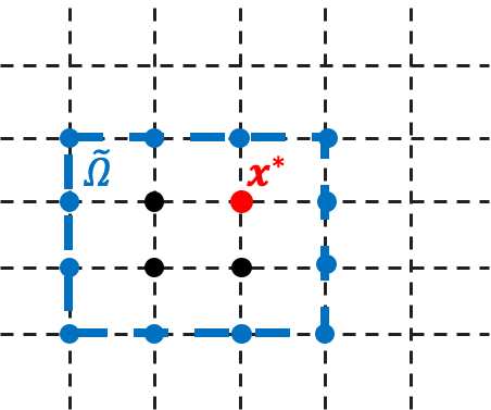
Figure 1: PDE in a local domain $\tilde{\Omega}$. A neural network $\tilde{\mathcal{G}}$ is trained to learn the mapping from all or some of $u(\mathbf{x})$ and $f(\mathbf{x})$ for $\mathbf{x}\in\tilde{\Omega}$ to $u(\mathbf{x}^{*})$.

The size and shape of $\tilde{\Omega}$ are also hyperparameters to be chosen. Because the network learns for a small local domain, by traversing the entire domain $\Omega$, we can generate many input-output pairs for training the network, which makes it possible to learn a network from only one PDE solution. We will compare the performance of several different choices of network inputs in our numerical experiments.

We first train a neural network $\tilde{\mathcal{G}}$ with the dataset $\mathcal{T}=\{(f_{\mathcal{T}},u_{\mathcal{T}})\}$. Using the pre-trained model $\tilde{\mathcal{G}}$, in the second stage of our method, we propose three approaches to predict the solution of a new $f=f_{0}+\Delta f$. Since the inputs of the pre-trained neural network also include the solution to be predicted, we cannot predict solution for $f$ directly.

Prediction via a fixed-point iteration (FPI).

We first propose a mesh-based iterative approach (Algorithm 1). Because $f$ is close to $f_{0}$,we use $u_{0}$ as the initial guess of $u$, and then in each iteration, we apply the trained network on the current solution as the input to get a new solution. When the solution is converged, $u$ and $f$ are consistent with respect to the local operator $\mathcal{G}$, and thus the current $u$ is the solution of our PDE.

1 Initiate: $u(\mathbf{x})\leftarrow u_{0}(\mathbf{x})$ for all $\mathbf{x}\in\Omega$;

2 while $u$ has not converged do

3       for $\mathbf{x}\in\Omega$ do

4             $\hat{u}(\mathbf{x})\leftarrow\tilde{\mathcal{G}}(\text{the inputs of }u\text{ and }f\text{ in }\tilde{\Omega}(x))$;

5             Apply boundary and initial conditions to $\hat{u}(\mathbf{x})$;

6            

7      Update: $u(\mathbf{x})\leftarrow\hat{u}(\mathbf{x})$ for all $\mathbf{x}\in\Omega$;

8      

Algorithm 1 Predicting the solution $u=\mathcal{G}(f)$ for a new $f$ via FPI.

Prediction via a local-solution-operator informed neural network (LOINN).

We also propose a neural-network based approach, which is meshfree and has more flexibility to handle boundary/initial conditions and training points inside the computationial domain. We construct a neural network that takes the coordinates $\mathbf{x}$ as the input, and output the approximated solution $\hat{u}(\mathbf{x})$. To train the network, we constraint $\hat{u}(\mathbf{x})$ on $\tilde{\mathcal{G}}$ via the loss function defined as the discrepancy between $\hat{u}(\mathbf{x})$ and $\tilde{\mathcal{G}}(\hat{u}\text{ and }f\text{ in }\tilde{\Omega}(\mathbf{x}))$:

$$\mathcal{L}=\frac{1}{|\mathcal{T}_{l}|}\sum_{\mathbf{x}\in\mathcal{T}_{l}}\left(\hat{u}(\mathbf{x})-\tilde{\mathcal{G}}(\hat{u}\text{ and }f\text{ in }\tilde{\Omega}(\mathbf{x}))\right)^{2}+\frac{1}{|\mathcal{T}_{b}|}\sum_{\mathbf{x}\in\mathcal{T}_{b}}\lVert\mathcal{B}(\hat{u}(\mathbf{x}),\mathbf{x})\lVert_{2}^{2}.$$

$\mathcal{T}_{l}$ and $\mathcal{T}_{b}$ are the data points in the domain constrained by the local solution operator $\tilde{\mathcal{G}}$ and on the boundary, respectively. The network architecture is shown in Fig. 4.

Prediction via a local-solution-operator informed neural network with correction (cLOINN).

To improve the performance of LOINN, we choose the approximated solution as $\hat{u}(\mathbf{x})=\mathcal{N}(\mathbf{x})+u_{0}(\mathbf{x})$, where $\mathcal{N}(\mathbf{x})$ is the neural network output. We show the architecture of cLOINN in Fig. 5.

3 Results

In this section, we show the effectiveness of our proposed method for a few problems, and compare the accuracy of different choices of the local solution operator $\tilde{\mathcal{G}}$ and training data. To generate the dataset $\mathcal{T}$, we use $f_{\mathcal{T}}(x)=f_{\text{random}}(x)+f_{0}(x)$, where $f_{\text{random}}(x)\sim\mathcal{GP}(0,k(x_{1},x_{2}))$ is randomly sampled from a mean-zero Gaussian random field (GRF) with the covariance kernel $k(x_{1},x_{2})=\sigma^{2}\exp(-\|x_{1}-x_{2}\|^{2}/2l^{2})$ ($\sigma$: standard deviation; $l$: correlation length). The numerical solution is obtained via the finite difference method in an equispaced dense grid with a grid size $h_{d}$. However, we learn $\mathcal{G}$ in a coarser grid with a step size $h_{c}$. The choices of $\sigma$, $l$, $h_{d}$, and $h_{c}$ for each example are listed in Table 2. After the pre-trained model $\tilde{\mathcal{G}}$ is obtained, we use FPI, LOINN, and cLOINN to predict a new $f=f_{0}+\Delta f$, in which $\Delta f$ is sampled from a GRF with a correlation length $l=0.1$ and different standard deviation $\sigma$. In this study, we only consider the structured equispaced grid to demonstrate our method, but LOINN and cLOINN allow us to randomly sample points in the domain and on the boundaries.

We first demonstrate the capability of our method by a pedagogical example of a one-dimensional Poisson equation in Appendix C.

3.1 Linear diffusion equation

The second equation we consider is a linear diffusion equation $\frac{\partial u}{\partial t}=D\frac{\partial^{2}u}{\partial x^{2}}+f(x)$ with zero boundary and initial conditions, where $D=0.01$ is the diffusion coefficient, and the solution operator is $\mathcal{G}:f\mapsto u$. We consider two candidate local solution operators (Fig. 2): (A) the simplest local domain with 4 nodes $\tilde{\mathcal{G}}_{1}$: $\{u(x_{i},t_{j-1}),u(x_{i-1},t_{j}),u(x_{i+1},t_{j}),f(x_{i},t_{j})\}\mapsto u(x_{i},t_{j})$, and (B) a larger local domain with 6 nodes $\tilde{\mathcal{G}}_{2}$: $\{u(x_{i-1},t_{j-1}),u(x_{i},t_{j-1}),u(x_{i+1},t_{j-1}),u(x_{i-1},t_{j}),$ $u(x_{i+1},t_{j}),f(x_{i},t_{j})\}\mapsto u(x_{i},t_{j})$.

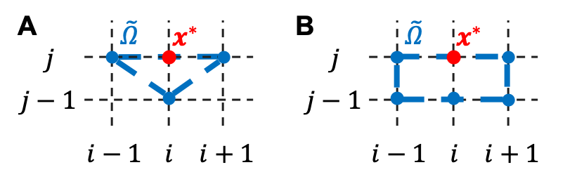
Figure 2: Local domains $\tilde{\Omega}$ of the linear diffusion-reaction equation. Domains with (A) 4 nodes and (B) 6 nodes.

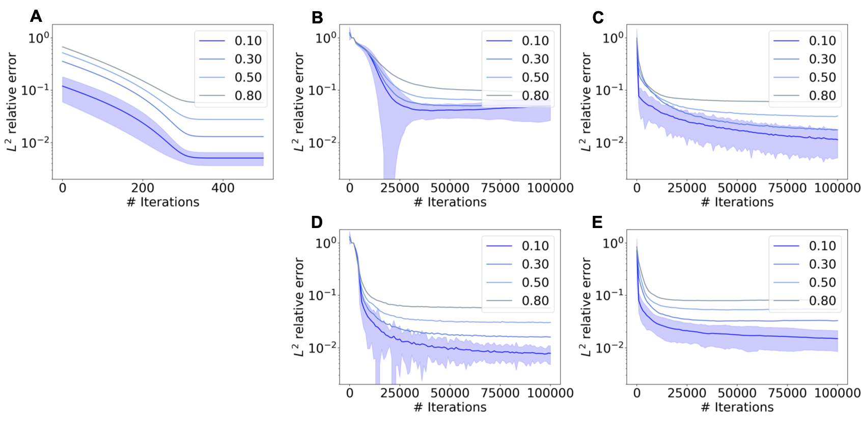
Figure 11: Learning solution of the linear diffusion equation. The $L^{2}$ relative errors tested on 100 random $\Delta f$ sampled from GRF of various $\sigma$ and $l=0.1$ with local operator (A to C) $\tilde{\mathcal{G}}_{1}$ and (D and E) $\tilde{\mathcal{G}}_{2}$. (A) FPI. (B and D) LOINN. (C and E) cLOINN.

We want to predict the solution for a new $f=0.9\sin(2\pi x)+\Delta f$. When we consider the local solution operator $\tilde{\mathcal{G}}_{1}$, for a fixed $\sigma$, FPI and cLOINN both work well and outperform LOINN (Table 1). When it comes to $\tilde{\mathcal{G}}_{2}$, LOINN and cLOINN give us stable results, but FPI diverges. We also observe that the errors increase when $\sigma$ is larger. The details of error convergence are shown in Figs. 10 and 11.

Table 1: $L^{2}$ relative errors of different approaches for linear diffusion equation test on 100 random $f$.

$\sigma$	FPI		LOINN		cLOINN
	$\tilde{\mathcal{G}}_{1}$	$\tilde{\mathcal{G}}_{2}$	$\tilde{\mathcal{G}}_{1}$	$\tilde{\mathcal{G}}_{2}$	$\tilde{\mathcal{G}}_{1}$	$\tilde{\mathcal{G}}_{2}$
0.10	0.51 $\pm$ 0.14%	-	4.95 $\pm$ 2.30%	0.78 $\pm$ 0.31%	1.14 $\pm$ 0.63%	1.49 $\pm$ 0.65%
0.30	1.30 $\pm$ 1.08%	-	5.06 $\pm$ 2.52%	1.15 $\pm$ 1.60%	1.76 $\pm$ 1.12%	3.31 $\pm$ 1.93%
0.50	2.77 $\pm$ 2.38%	-	6.35 $\pm$ 2.52%	3.05 $\pm$ 2.51%	3.23 $\pm$ 2.49%	5.56 $\pm$ 2.99%
0.80	5.82 $\pm$ 6.31%	-	9.22 $\pm$ 5.64%	5.78 $\pm$ 6.60%	6.39 $\pm$ 7.73%	8.87 $\pm$ 7.62%

3.2 Nonlinear diffusion-reaction equation

We consider a nonlinear diffusion-reaction equation with a source term $f(x)$: $\frac{\partial{u}}{\partial{t}}=D\frac{\partial^{2}u}{\partial x^{2}}+ku^{2}+f(x),x\in[0,1],t\in[0,1],$ with zero initial and boundary conditions, where $D=0.01$ is the diffusion coefficient, and $k=0.01$ is the reaction rate. The solution operator is the mapping from $f(x)$ to $u(x,t)$.

We use the same $\tilde{\mathcal{G}}_{1}$ as the previous example. In this experiment, the numerical solutions are obtained from a denser grid of 1001$\times$1001, but we learn $\tilde{\mathcal{G}}_{1}$ on a coarser grid of 101$\times$101, 51$\times$51, 26$\times$26, 21$\times$21, or 16$\times$16. Here $f_{0}=0.9\sin(2\pi x)$. We use FPI, LOINN and cLOINN, and compare $L^{2}$ relative errors with different $\sigma$ and resolutions. With higher resolution, all approaches perform better (Fig. 3). The errors can achieve approximately 10% even on a coarser grid of 21$\times$21 (Tables 5, 6, 7, 8, and 9), which demonstrates the robustness and generalizability of our proposed method.

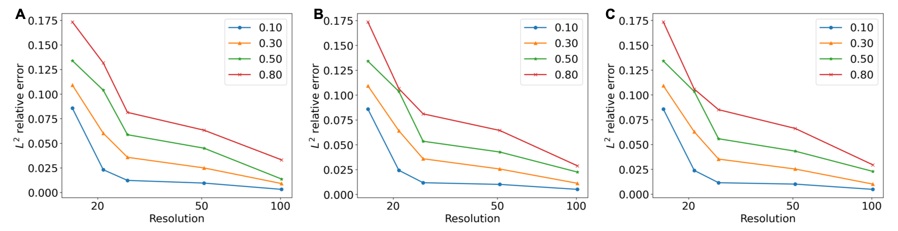
Figure 3: $L^{2}$ relative error of different test functions with $\sigma=0.10,0.30,0.50,0.80$ when using different grid resolution for the nonlinear diffusion-reaction equation. (A) FPI. (B) LOINN. (C) cLOINN.

4 Conclusions

Learning solution operators of partial differential equations (PDEs) usually requires a large amount of training data. In this study, we propose, to the best of our knowledge, the first one-shot method to learn solution operators from only one PDE solution. In future, we will carry out further validation on different types of PDEs, extend the method to unstructured meshes, and improve our approaches for faster convergence and better computational efficiency.

Broader impacts

In this paper, we propose the first one-shot method to learn solution operators of PDEs. With only one data point, our work points out a direction to improve and accelerate scientific research related to discovering governing equations of physics systems. In the meanwhile, when employing our method, we also need to consider ethical implications and prevent abusing machine learning technologies in applications of science and engineering.

Appendix A Schematic of LOINN and cLOINN

Figs. 4 and 5.

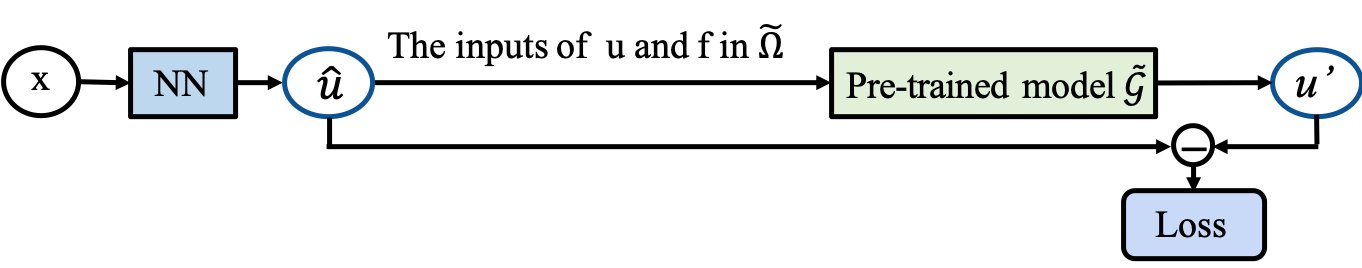
Figure 4: The architecture of LOINN.

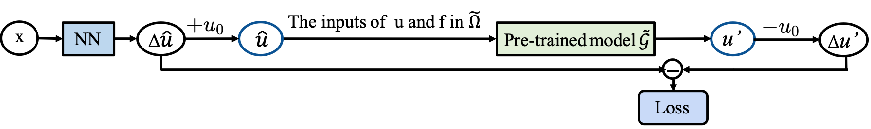
Figure 5: The architecture of cLOINN.

Appendix B Hyperparameters

Tables 2 and 3.

Table 2: Hyperparameters for numerical experiments.

	Appendix C	Section 3.1	Section 3.2
$l$	0.01	0.01	0.01
$\sigma$	0.5	0.1	0.1
$h_{d}$	0.1	0.1	0.1
$h_{c}$	0.01	0.01	0.01, 0.02, 0.04, 0.05, 0.07

Table 3: Hyperparameters of the neural networks.

		Depth	Width	Optimizer	#Iterations
Appendix C	$\tilde{\mathcal{G}}_{1}$	2	64	Adam + L-BFGS	200000
	$\tilde{\mathcal{G}}_{2}$	2	32	Adam + L-BFGS	200000
Section 3.1	$\tilde{\mathcal{G}}_{1}$	2	32	Adam + L-BFGS	100000
	$\tilde{\mathcal{G}}_{2}$	2	32	Adam + L-BFGS	100000
Section 3.2	$\tilde{\mathcal{G}}$	2	64	Adam + L-BFGS	150000

Appendix C 1D Poisson equation

In this section, we consider a pedagogical example of a one-dimensional Poisson equation $\Delta u=f(x),\quad x\in[0,1]$, with the zero Dirichlet boundary condition $u(0)=u(1)=0$, and the solution operator is $\mathcal{G}:f\mapsto u$. We choose the simplest local operator $\tilde{\mathcal{G}}_{1}$: $\{u(x_{i-1}),u(x_{i+1}),f(x_{i})\}\mapsto u(x_{i})$ and $\tilde{\mathcal{G}}_{2}$: $\{u(x_{i-1}),u(x_{i+1}),f(x_{i-1}),f(x_{i+1}),f(x_{i})\}$ $\mapsto u(x_{i})$ with 3 nodes. The training dataset $\mathcal{T}$ only has one data point $(f_{\mathcal{T}},\mathcal{G}(f_{\mathcal{T}}))$, and one example of $\mathcal{T}$ is shown in Fig. 6.

We assume that we have the solution $u_{0}$ for $f_{0}=\sin(2\pi x)$. We show examples of $f=f_{0}+\Delta f$ in Fig. 7, and the black solid line is $f_{0}$. When $\sigma$ is larger, there is a greater difference between $f_{0}$ and $f$. We report the geometric mean of $L^{2}$ relative errors of all cases in Table 4. The comparison of results using different $\sigma$ is shown in Fig. 8. When $\sigma=0.02$, all approaches reached $L^{2}$ relative error of about $0.1\%$. It is observed that in this experiment the local solution operator $\tilde{\mathcal{G}}_{1}$ outperforms $\tilde{\mathcal{G}}_{2}$ from Fig. 9. As expected, when $\sigma$ is smaller, the performance is better. cLOINN outperforms LOINN, and performs as well as FPI.

Table 4: $L^{2}$ relative errors of different approaches for 1D Poisson equation test on 100 random $\Delta f$.

$\sigma$	FPI		LOINN		cLOINN
	$\tilde{\mathcal{G}}_{1}$	$\tilde{\mathcal{G}}_{2}$	$\tilde{\mathcal{G}}_{1}$	$\tilde{\mathcal{G}}_{2}$	$\tilde{\mathcal{G}}_{1}$	$\tilde{\mathcal{G}}_{2}$
0.02	0.83 $\pm$ 0.59%	1.13 $\pm$ 0.43%	0.90 $\pm$ 0.59%	1.14 $\pm$ 0.43%	0.79 $\pm$ 0.55%	1.12 $\pm$ 0.43%
0.05	1.90 $\pm$ 1.79%	1.79 $\pm$ 1.39%	1.90 $\pm$ 1.79%	1.83 $\pm$ 1.41%	1.87 $\pm$ 1.80%	1.78 $\pm$ 1.39%
0.10	3.88 $\pm$ 3.64%	3.73 $\pm$ 2.97%	3.90 $\pm$ 3.64%	3.82 $\pm$ 2.94%	3.94 $\pm$ 4.24%	3.74 $\pm$ 2.97%
0.15	6.09 $\pm$ 6.07%	6.10 $\pm$ 4.70%	6.10 $\pm$ 6.07%	6.08 $\pm$ 4.71%	6.20 $\pm$ 6.34%	6.18 $\pm$ 7.86%

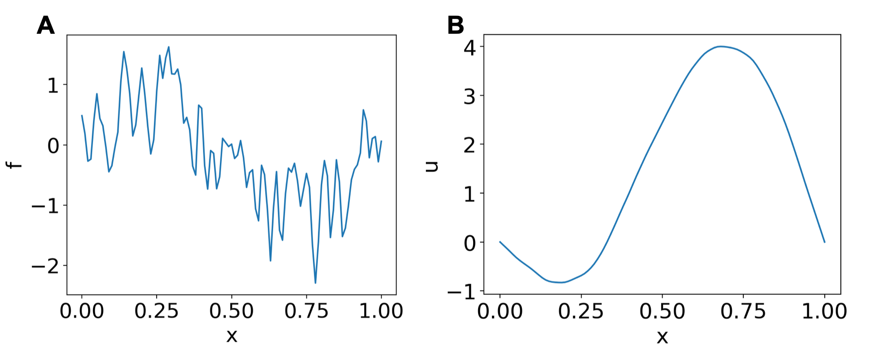
Figure 6: One example of the training data for the 1D Poisson equation. (A) A random $f_{\mathcal{T}}$ generated from GRF. (B) The corresponding solution $u_{\mathcal{T}}$.

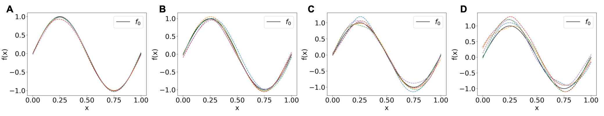
Figure 7: Examples of some random $f=f_{0}+\Delta f$ with $\Delta f$ sampled from GRF of different $\sigma$ and $l=0.1$. (A) $\sigma=0.02$. (B) $\sigma=0.05$. (C) $\sigma=0.10$. (C) $\sigma=0.15$.

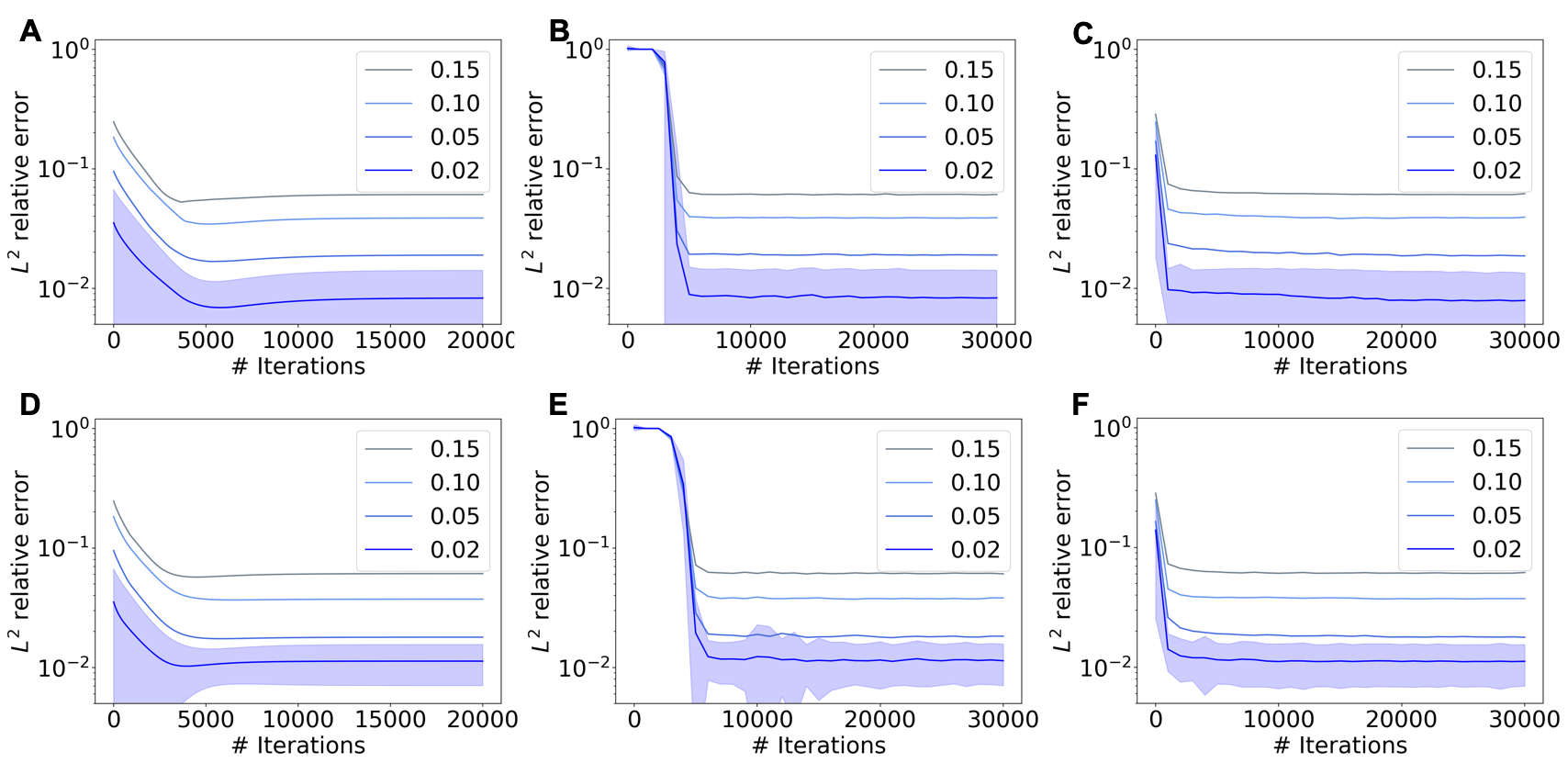
Figure 8: Learning solution of the 1D Poisson equation. The $L^{2}$ relative errors tested on 100 random $\Delta f$ sampled from GRF of various $\sigma$ and $l=0.1$ with local operator (A to C) $\tilde{\mathcal{G}}_{1}$ and (D to F) $\tilde{\mathcal{G}}_{2}$. (A and D) FPI. (B and E) LOINN. (C and F) cLOINN.

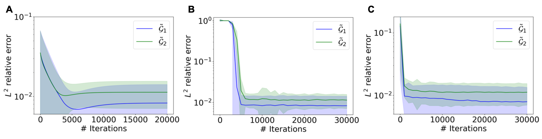
Figure 9: Learning solution of the 1D Poisson equation with different local operators $\tilde{\mathcal{G}}$. The $L^{2}$ relative errors tested on 100 random $\Delta f$ sampled from GRF of $\sigma=0.02$ and $l=0.1$ using (A) FPI, (B) LOINN, and (C) cLOINN.

Appendix D Linear diffusion equation

Fig. 10 and Table 5.

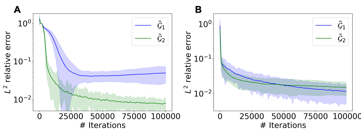
Figure 10: Learning solution of the linear diffusion equation with different local operators $\tilde{\mathcal{G}}$. The $L^{2}$ relative errors tested on 100 random $f$ sampled from GRF of $\sigma=0.10$ and $l=0.1$ using (A) LOINN and (B) cLOINN.

Appendix E Nonlinear diffusion-reaction equation

Tables 5, 6, 7, 8 and 9.

Table 5: $L^{2}$ relative errors of different approaches for nonlinear diffusion-reaction equation test on 100 random $\Delta f$. We learn the local operator on a coarser mesh size of 101.

$\sigma$	FPI	LOINN	cLOINN
0.10	0.32 $\pm$ 0.08%	0.52 $\pm$ 0.20%	0.49 $\pm$ 0.21%
0.30	0.91 $\pm$ 0.51%	1.13 $\pm$ 0.60%	1.02 $\pm$ 0.62%
0.50	1.81 $\pm$ 1.37%	2.26 $\pm$ 1.46%	2.30 $\pm$ 1.52%
0.80	3.32 $\pm$ 3.54%	2.89 $\pm$ 2.16%	2.96 $\pm$ 2.39%

Table 6: $L^{2}$ relative errors of different approaches for nonlinear diffusion-reaction equation test on 100 random $f$. We learn the local operator on a coarser mesh size of 51.

$\sigma$	FPI	LOINN	cLOINN
0.10	0.96 $\pm$ 0.30%	1.02 $\pm$ 0.30%	1.02 $\pm$ 0.29%
0.30	2.50 $\pm$ 0.78%	2.57 $\pm$ 0.77%	2.54 $\pm$ 0.78%
0.50	4.21 $\pm$ 1.47%	4.28 $\pm$ 1.46%	4.34 $\pm$ 1.52%
0.80	6.34 $\pm$ 2.59%	6.45 $\pm$ 2.57%	6.63 $\pm$ 2.94%

Table 7: $L^{2}$ relative errors of different approaches for nonlinear diffusion-reaction equation test on 100 random $f$. We learn the local operator on a coarser mesh size of 26.

$\sigma$	FPI	LOINN	cLOINN
0.10	1.23 $\pm$ 0.35%	1.19 $\pm$ 0.34%	1.16 $\pm$ 0.34%
0.30	3.58 $\pm$ 1.27%	3.60 $\pm$ 1.25%	3.54 $\pm$ 1.29%
0.50	5.88 $\pm$ 1.94%	5.36 $\pm$ 1.85%	5.59 $\pm$ 1.84%
0.80	8.15 $\pm$ 3.26%	8.12 $\pm$ 3.50%	8.52 $\pm$ 4.18%

Table 8: $L^{2}$ relative errors of different approaches for nonlinear diffusion-reaction equation test on 100 random $f$. We learn the local operator on a coarser mesh size of 21.

$\sigma$	FPI	LOINN	cLOINN
0.10	2.32 $\pm$ 0.59%	2.44 $\pm$ 0.64%	2.40 $\pm$ 0.67%
0.30	6.03 $\pm$ 2.06%	6.42 $\pm$ 1.92%	6.29 $\pm$ 1.94%
0.50	10.41 $\pm$ 3.40%	10.38 $\pm$ 4.13%	10.35 $\pm$ 4.29%
0.80	13.18 $\pm$ 4.94%	10.66 $\pm$ 4.37%	10.59 $\pm$ 4.52%

Table 9: $L^{2}$ relative errors of different approaches for nonlinear diffusion-reaction equation test on 100 random $f$. We learn the local operator on a coarser mesh size of 16.

$\sigma$	FPI	LOINN	cLOINN
0.10	8.58 $\pm$ 0.27%	8.60 $\pm$ 0.27%	8.58 $\pm$ 0.27%
0.30	10.93 $\pm$ 1.84%	10.94 $\pm$ 1.85%	10.93 $\pm$ 1.84%
0.50	13.41 $\pm$ 3.51%	13.42 $\pm$ 3.41%	13.42 $\pm$ 3.40%
0.80	17.35 $\pm$ 5.26%	17.37 $\pm$ 5.25%	17.36 $\pm$ 5.26%

References

- [1] G. Pang, L. Lu, and G. E. Karniadakis. fPINNs: Fractional physics-informed neural networks. SIAM Journal on Scientific Computing, 41(4):A2603–A2626, 2019.
- [2] D. Zhang, L. Lu, L. Guo, and G. E. Karniadakis. Quantifying total uncertainty in physics-informed neural networks for solving forward and inverse stochastic problems. Journal of Computational Physics, 397:108850, 2019.
- [3] Y. Chen, L. Lu, G. E. Karniadakis, and L. Dal Negro. Physics-informed neural networks for inverse problems in nano-optics and metamaterials. Optics Express, 28(8):11618–11633, 2020.
- [4] A. Yazdani, L. Lu, M. Raissi, and G. E. Karniadakis. Systems biology informed deep learning for inferring parameters and hidden dynamics. PLoS Computational Biology, 16(11):e1007575, 2020.
- [5] C. Rao, H. Sun, and Y. Liu. Physics-informed deep learning for incompressible laminar flows. Theoretical and Applied Mechanics Letters, 10(3):207–212, 2020.
- [6] J. Wu, H. Xiao, and E. Paterson. Physics-informed machine learning approach for augmenting turbulence models: A comprehensive framework. Physical Review Fluids, 3(7):074602, 2018.
- [7] E. Qian, B. Kramer, B. Peherstorfer, and K. Willcox. Lift & learn: Physics-informed machine learning for large-scale nonlinear dynamical systems. Physica D: Nonlinear Phenomena, 406:132401, 2020.
- [8] L. Lu, X. Meng, Z. Mao, and G. E. Karniadakis. DeepXDE: A deep learning library for solving differential equations. SIAM Review, 63(1):208–228, 2021.
- [9] S. L. Brunton, J. L. Proctor, and J. N. Kutz. Discovering governing equations from data by sparse identification of nonlinear dynamical systems. Proceedings of the National Academy of Sciences, 113(15):3932–3937, 2016.
- [10] S. H. Rudy, S. L. Brunton, J. L. Proctor, and J. N. Kutz. Data-driven discovery of partial differential equations. Science Advances, 3(4):e1602614, 2017.
- [11] Z. Chen, Y. Liu, and H. Sun. Deep learning of physical laws from scarce data. arXiv preprint arXiv:2005.03448, 2020.
- [12] L. Lu, P. Jin, G. Pang, Z. Zhang, and G. E. Karniadakis. Learning nonlinear operators via DeepONet based on the universal approximation theorem of operators. Nature Machine Intelligence, 3(3):218–229, 2021.
- [13] L. Lu, X. Meng, S. Cai, Z. Mao, S. Goswami, Z. Zhang, and G. E. Karniadakis. A comprehensive and fair comparison of two neural operators (with practical extensions) based on FAIR data. Computer Methods in Applied Mechanics and Engineering, 393:114778, 2022.
- [14] P. Jin, S. Meng, and L. Lu. MIONet: Learning multiple-input operators via tensor product. arXiv preprint arXiv:2202.06137, 2022.
- [15] Z. Li, N. Kovachki, K. Azizzadenesheli, B. Liu, K. Bhattacharya, A. Stuart, and A. Anandkumar. Fourier neural operator for parametric partial differential equations. arXiv preprint arXiv:2010.08895, 2020.
- [16] H. Wang, Z. Zhao, and Y. Tang. An effective few-shot learning approach via location-dependent partial differential equation. Knowledge and Information Systems, pages 1–21, 2019.
- [17] C. Fang, Z. Zhao, P. Zhou, and Z. Lin. Feature learning via partial differential equation with applications to face recognition. Pattern Recognition, 69:14–25, 2017.