Dispersive Estimates for Nonlinear Schrödinger Equations with External Potentials

Abstract.

We consider the long time dynamics of nonlinear Schrödinger equations with an external potential. More precisely, we look at Hartree type equations in three or higher dimensions with small initial data. We prove an optimal decay estimate, which is comparable to the decay of free solutions. Our proof relies on good control on a high Sobolev norm of the solution to estimate the terms in Duhamel’s formula.

1. Introduction

Nonlinear Schrödinger equations are of great interest in physics and mathematics, see [1, 2, 3] for an overview. They are used to model waves on the surface of a deep fluid, see [4], to describe Langmuir waves in plasma physics, see [5], and they are used in nonlinear optics, see [6]. Furthermore, these equations describe intramolecular vibrations in $\alpha$-helices in proteins, see [7, 3]. The condensate in Bose-Einstein condensation can also be described by nonlinear Schrödinger equations via the mean-field approximation, which are usually called Hartree or Gross-Pitaevskii equations, see [8, 9, 10, 11].

We consider the nonlinear Schrödinger equation with a Hartree type nonlinearity

$$\begin{cases}\mathrm{i}\partial_{t}u&=-\Delta u+Vu+(w*|u|^{2})u\\ u(0)&=u_{0}\end{cases}$$ (1)

in dimension $d\geq 3$ with an external potential $V:\mathbb{R}^{d}\to\mathbb{R}$ and an interaction potential $w:\mathbb{R}^{d}\to\mathbb{R}$. We call this equation a Hartree type equation. For $V,w$ nice enough and small initial data $u_{0}$, we show the decay estimate

$$||u(t)||_{\infty}\leq\frac{C}{(1+|t|)^{\frac{d}{2}}}$$ (2)

for a constant $C>0$, where $C$ depends on $w$ only in terms of $||w||_{1}$. For $p\in[1,\infty]$, we denote by $||\cdot||_{p}$ the $L^{p}$ norm on $\mathbb{R}^{d}$. Such a decay estimate was proved in [12, Corollary 3.4] for $d=3$, $V=0$ and even large initial data. The decay estimate from [12] was used in [12, 13] to understand the dynamics of many-body quantum systems in the context of Bose-Einstein condensation in dimension $d=3$ without an external potential. It should be possible to use our decay estimate to get similar results in the weak coupling regime in dimension $d\geq 3$ with an external potential $V$.

Linear equation. To get a better understanding why we might expect a decay estimate of the form (2) for nonlinear Schrödinger equations under certain conditions, let us look at the linear Schrödinger equation

$$\begin{cases}\mathrm{i}\partial_{t}u&=-\Delta u\\ u(0)&=u_{0}\end{cases}$$ (3)

with initial data $u_{0}\in L^{1}(\mathbb{R}^{d})\cap L^{2}(\mathbb{R}^{d})$. The solution to this equation, see for example [14, Equation (4.2)], is given by

$$u(t,x)=\left(e^{-\mathrm{i}t(-\Delta)}u_{0}\right)(x)=\frac{1}{(4\pi\mathrm{i}t)^{\frac{d}{2}}}\int_{\mathbb{R}^{d}}\mathrm{d}{y}\,e^{\frac{\mathrm{i}|x-y|^{2}}{4t}}u_{0}(y)\,.$$ (4)

By taking the $L^{\infty}$ norm on both sides, we obtain the decay estimate

$$||u(t)||_{\infty}\leq\frac{1}{(4\pi)^{\frac{d}{2}}}\frac{1}{|t|^{\frac{d}{2}}}||u_{0}||_{1}\,.$$ (5)

This decay rate agrees with the decay rate in equation (2) for large times $t$. Note that the estimate (2) is even stronger than (5) for small times $t$, which will follow from our assumptions on the initial data.

Nonlinear Schrödinger equations without external potentials. The equation (1) with $V=0$, namely

$$\begin{cases}\mathrm{i}\partial_{t}u&=-\Delta u+(w*|u|^{2})u\\ u(0)&=u_{0}\end{cases}$$ (6)

has been studied extensively in the literature. There are many results on local or global existence and uniqueness, scattering, modified scattering and wave operators for these equations. Strauss studied scattering theory in a general setting and applied it to nonlinear Schrödinger equations, see [15, 16]. For Hartree type nonlinearities with repulsive interaction potential $w$, Ginibre and Velo proved the decay estimate

$$||u(t)||_{q}\leq C(1+|t|)^{-\frac{d}{2}\left(\frac{1}{q^{\prime}}-\frac{1}{q}\right)}$$ (7)

for all $q$ such that $\left[\frac{1}{2}-\frac{1}{d}\right]_{+}\leq\frac{1}{q}\leq\frac{1}{2}$, see [17, Theorem 6.1(1)]. Note that $q=\infty$ is not allowed here if $d\geq 3$. We would also like to mention [18, 19, 20, 21, 22, 23]. More recent results include [24, 25, 26].

Let us now discuss some results and the corresponding proof ideas, which will be important for the proof of our main result.

Hayashi and Naumkin were the first to prove a decay estimate of the form (2) for critical nonlinearities and small initial data, see [27]. The nonlinearities they considered were

$$\lambda|u|^{\frac{2}{d}}u+\mu|u|^{\eta-1}u$$ (8)

in $d\in\{1,2,3\}$ with $\eta-1>\frac{2}{d}$, $\lambda,\mu\in\mathbb{R}$ and

$$\lambda(|\cdot|^{-1}*|u|^{2})u+\mu(|\cdot|^{-\delta}*|u|^{2})u$$ (9)

in $d\geq 2$ with $1<\delta<d$, $\lambda,\mu\in\mathbb{R}$. Moreover, they proved modified scattering for these equations.

Kato and Pusateri provided an alternative proof of the result in [27] for the local nonlinearity $\pm|u|^{2}u$ in $d=1$ and the Hartree type nonlinearity $\pm(|\cdot|^{-1}*|u|^{2})u$ in $d\geq 2$ in [28]. They defined a quantity $||u||_{X_{T}}$ depending on a time parameter $T\geq 0$ and they proved an estimate of the form $||u||_{X_{T}}\leq\varepsilon+C||u||_{X_{T}}^{3}$, where $\varepsilon>0$ is small and both $\varepsilon,C$ are independent of $T$. They used this inequality to deduce that $\sup_{T\geq 0}||u||_{X_{T}}<\infty$ for small initial data. Their proof relied on a careful analysis of the equation in the Fourier space.

For the Hartree type equation with non-negative, spherically symmetric and decreasing $w\in L^{1}(\mathbb{R}^{d})\cap C^{1}_{0}(\mathbb{R}^{d})$, Grillakis and Machedon showed a decay estimate of the form (2) for initial data $u_{0}\in W^{k,1}(\mathbb{R}^{d})$ for $k$ sufficiently large, see [12, Corollary 3.4]. It is worth pointing out that their result holds for large initial data. Their result was applied in [12, 13] in the context of Bose-Einstein condensation to show a norm approximation for the dynamics. Another more recent result on the dynamics of many-body quantum systems, which we would like to mention, is [29].

Nonlinear Schrödinger equations with external potentials. We start by looking at results in dimension $d=1$. Cuccagna, Georgiev and Visciglia proved a decay estimate of the form (2) and scattering for small initial data and a nonlinearity of the form $\pm|u|^{p-1}u$ for $3<p<5$, see [30]. Germain, Pusateri and Rousset considered the nonlinearity $\pm|u|^{p-1}u$ with $p=3$, see [31]. They proved a decay estimate of the form (2) and modified scattering for small initial data. In their proof, they used the distorted Fourier transform and they carefully analysed an oscillatory integral.

Naumkin considered the cubic nonlinear Schrödinger equation with an external potential and proved a decay estimate of the form (2) and modified scattering using the distorted Fourier transform, see [32, 33].

Martinez proved decay in the sense that $\lim_{n\to\infty}||u(t)||_{L^{\infty}(I)}=0$ for any bounded interval $I\subset\mathbb{R}$ for small odd solutions $u$ to nonlinear Schrödinger equations with even external potentials $V$, see [34]. The nonlinearities considered in [34] are of the form $f(|u|^{2})u$ for a function $f:\mathbb{R}\to\mathbb{R}$ with $|f(s)|\lesssim s^{\frac{p-1}{2}}$ for $1<p<5$ and Hartree type nonlinearities $\pm\left(|\cdot|^{-\alpha}*|u|^{2}\right)u$ for $0<\alpha<1$.

Let us now mention some results in dimension $d=3$. Pusateri and Soffer proved a decay estimate of the form $||u(t)||_{\infty}\leq C(1+|t|)^{-(1+\alpha)}$ for some $\alpha>0$ for the nonlinear Schrödinger equation with nonlinearity $-u^{2}$ and small initial data, see [35]. In a similar way to [31], the proof in [35] relies on the distorted Fourier transform and a careful analysis of an oscillatory integral.

Hong proved scattering in $H^{1}$ for the cubic focusing nonlinear Schrödinger equation with an external potential $V$ with small negative part, see [36]. Hong’s proof strategy was to show that there are no minimal blow-up solutions. Nakanishi classified the dynamics of solutions to the cubic nonlinear Schrödinger equation with small initial data and a radial external potential $V$, which is such that the operator $-\Delta+V$ has exactly one negative eigenvalue, see [37].

There are only few decay results for nonlinear Schrödinger equations with external potentials in $d=3$. Note that the results in $d=3$, which we mentioned here, treat local nonlinearities. Nonlinear Schrödinger equations with non-local nonlinearities such as the Hartree type equation, which we consider below, are not necessarily easier to deal with.

1.1. Main result

Our main result is a decay estimate of the form (2) for the Hartree type equation with small initial data in dimension $d\geq 3$.

Theorem 1.1 (Dispersive estimates for the Hartree type equation in $d\geq 3$ for small initial data).

Let $d\geq 3$ and let $k\in\mathbb{N}$ be the smallest even number with $k>\frac{d}{2}$. Let $V\in W^{k,\infty}(\mathbb{R}^{d})$ be a real-valued function and satisfy

$$||e^{-\mathrm{i}t(-\Delta+V)}f||_{\infty}\leq C^{V}|t|^{-\frac{d}{2}}||f||_{1}$$ (10)

for every $f\in L^{1}(\mathbb{R}^{d})\cap L^{2}(\mathbb{R}^{d})$ and some constant $C^{V}\geq 1$. Let the interaction potential $w\in L^{1}(\mathbb{R}^{d})\cap L^{\frac{d}{2}}(\mathbb{R}^{d})$ be an even, real-valued function. Let $u_{0}\in H^{k}(\mathbb{R}^{d})$ and let $u\in C\left(\mathbb{R},H^{2}(\mathbb{R}^{d})\right)\cap C\left(\mathbb{R},H^{-1}(\mathbb{R}^{d})\right)$ be the unique global strong solution to the Hartree type equation

$$\begin{cases}\mathrm{i}\partial_{t}u&=(-\Delta+V)u+(w*|u|^{2})u\\ u(0)&=u_{0}\end{cases}$$ (11)

given by Theorem 2.11. Assume that the initial data is sufficiently small, that is,

$$||e^{\mathrm{i}(-\Delta+V)}u_{0}||_{1}\,,||u_{0}||_{H^{k}}\leq\varepsilon_{0}$$ (12)

for some $\varepsilon_{0}=\varepsilon_{0}(d,V,||w||_{1})>0$. Then there exists a constant $C_{0}=C_{0}(d,V,||w||_{1})>0$ such that

$$||u(t)||_{\infty}\leq\frac{C_{0}}{(1+|t|)^{\frac{d}{2}}}$$ (13)

for all $t\geq 0$. Furthermore, if we assume that

$$||e^{\mathrm{i}(-\Delta+V)}(\partial_{t}u)(0)||_{1}\,,||(\partial_{t}u)(0)||_{H^{k}}\leq\tilde{\varepsilon}_{0}$$ (14)

for some $\tilde{\varepsilon}_{0}=\tilde{\varepsilon}_{0}(d,V,||w||_{1})>0$, then

$$||\partial_{t}u(t)||_{\infty}\leq\frac{\tilde{C}_{0}}{(1+|t|)^{\frac{d}{2}}}$$ (15)

for all $t\geq 0$, where $\tilde{C}_{0}=\tilde{C}_{0}(d,V,||w||_{1})>0$.

This result is new even when $d=3$.

Remark 1.2.

A special case of Theorem 1.1 was proved by Grillakis and Machedon [12, Corollary 3.4], where they considered $V=0$ in dimension $d=3$. Their result even holds for large initial data.

Remark 1.3 (Application in many-body quantum mechanics).

Note that the $w$-dependence of the constants $\varepsilon_{0}$ and $C_{0}$ is only in terms of $||w||_{1}$. For proving the norm approximation for the dynamics of many-body quantum systems in dimension $d=3$ without an external potential in [12, 13], it was crucial that the constants in the decay estimate in [12, Corollary 3.4] depended on $w$ only in terms of $||w||_{1}$. Using Theorem 1.1, it should be possible to prove analogous results in the small coupling regime for the many-body Schrödinger equation with an external potential $V$ in dimension $d\geq 3$.

Remark 1.4 (Dispersive estimates for $e^{-\mathrm{i}t(-\Delta+V)}$).

In Theorem 2.1, we mention two different conditions under which a dispersive estimate of the form $||e^{-\mathrm{i}t(-\Delta+V)}f||_{\infty}\leq C^{V}|t|^{-\frac{d}{2}}||f||_{1}$ is satisfied.

Remark 1.5 (Extensions of Theorem 1.1).

• A similar decay result holds for $t\leq 0$. For that case, we need to replace the condition $||e^{\mathrm{i}(-\Delta+V)}u_{0}||_{1}\leq\varepsilon_{0}$ by $||e^{-\mathrm{i}(-\Delta+V)}u_{0}||_{1}\leq\varepsilon_{0}$ and $||e^{\mathrm{i}(-\Delta+V)}(\partial_{t}u)(0)||_{1}\leq\tilde{\varepsilon}_{0}$ by $||e^{-\mathrm{i}(-\Delta+V)}(\partial_{t}u)(0)||_{1}\leq\tilde{\varepsilon}_{0}$.

• In Remark 4.1, we treat the case of large initial data, which will be proved using Gronwall’s lemma. However, we will need the additional assumptions that $\lim_{t\to\infty}||u(t)||_{\infty}=0$ and $\sup_{t\geq 0}||D^{k}u(t)||_{\infty}<\infty$.

Remark 1.6 (Further questions).

• It would be interesting to consider the Hartree equation with an external potential $V\neq 0$, where the interaction potential $w$ is given by $w(x)=\frac{1}{|x|}$. The proof of a decay estimate of the form (13) for the Hartree equation with $V=0$ in [28] relied on a careful analysis in Fourier space. Similar to [35], one could try to use an approach involving a distorted Fourier transform for the Hartree equation with an external potential $V\neq 0$.

• An even more challenging problem is to understand the dynamics of solutions to the Hartree equation for large initial data with an external potential $V(x)=-\frac{Z}{|x|}$, where $Z>0$, which is closely linked to the dynamical ionisation conjecture, see [38].

An analogous result to Theorem 1.1 for the cubic nonlinear Schrödinger equation is the following theorem.

Theorem 1.7 (Dispersive estimates for the cubic nonlinear Schrödinger equation for small initial data).

Let $d\geq 3$ and suppose that the assumptions on the external potential $V$ and the smallness assumptions on the initial data $u_{0}$ from Theorem 1.1 are satisfied. Let $u$ be a global solution to either the focusing or the defocusing cubic nonlinear Schrödinger equation

$$\begin{cases}\mathrm{i}\partial_{t}u&=-\Delta u+Vu\pm|u|^{2}u\\ u(0)&=u_{0}\,.\end{cases}$$ (16)

Then the dispersive estimates

$$||u(t)||_{\infty}\leq\frac{C_{0}}{(1+|t|)^{\frac{d}{2}}}$$ (17)

and

$$||\partial_{t}u(t)||_{\infty}\leq\frac{\tilde{C}_{0}}{(1+|t|)^{\frac{d}{2}}}$$ (18)

hold for all for all $t\geq 0$ and some constants $C_{0}=C_{0}(d,V)>0$ and $\tilde{C}_{0}=\tilde{C}_{0}(d,V)>0$.

Remark 1.8 (The cubic nonlinear Schrödinger equation as a limit of Hartree type equations).

We can view the cubic nonlinear Schrödinger equation as a limit of Hartree type equations with interaction potentials $w$ that converge in the distributional sense to the delta distribution $\delta_{0}$ or $-\delta_{0}$, respectively. Moreover, the $w$-dependence of the constant $C_{0}$ in Theorem 1.1 is only in terms of $||w||_{1}$. For these two reasons, it is natural to expect that a result such as Theorem 1.7 holds if Theorem 1.1 is true, which is the corresponding result for Hartree type equations. At the end of Section 4, we explain two different strategies for proving Theorem 1.7.

1.2. Proof strategy

In this subsection, we describe our proof strategy for the estimate

$$||u(t)||_{\infty}\leq\frac{C_{0}}{(1+|t|)^{\frac{d}{2}}}$$ (19)

in Theorem 1.1. The proof idea is a combination of the proof ideas in [12] and [28]. The constants $C>0$ in this subsection can change from line to line but they do not depend on $t$ or $u$. Define $H:=-\Delta+V$.

By Duhamel’s formula, see Lemma 2.12, we have

$$u(t)=e^{-\mathrm{i}tH}u_{0}-\mathrm{i}\int_{0}^{t}\mathrm{d}{s}\,e^{-\mathrm{i}(t-s)H}(w*|u(s)|^{2})u(s)\,.$$ (20)

Taking the $L^{\infty}$ norm on both sides and using the dispersive estimate for $e^{-\mathrm{i}tH}$ of the form $||e^{-\mathrm{i}tH}f||_{\infty}\leq C|t|^{-\frac{d}{2}}||f||_{1}$, we get for $t\geq 0$

$$||u(t)||_{\infty} \leq||e^{-\mathrm{i}tH}u_{0}||_{\infty}+\int_{0}^{t}\mathrm{d}{s}\,||e^{-\mathrm{i}(t-s)H}(w*|u(s)|^{2})u(s)||_{\infty}$$

$$\leq||e^{-\mathrm{i}(t+1)H}e^{\mathrm{i}H}u_{0}||_{\infty}+\int_{0}^{t}\mathrm{d}{s}\,C|t-s|^{-\frac{d}{2}}||(w*|u(s)|^{2})u(s)||_{1}$$

$$\leq C|t+1|^{-\frac{d}{2}}||e^{\mathrm{i}H}u_{0}||_{1}+C\int_{0}^{t}\mathrm{d}{s}\,|t-s|^{-\frac{d}{2}}||w||_{1}||u(s)||_{2}^{2}||u(s)||_{\infty}$$

$$\leq C(1+|t|)^{-\frac{d}{2}}||e^{\mathrm{i}H}u_{0}||_{1}+C||w||_{1}||u_{0}||_{2}^{2}\int_{0}^{t}\mathrm{d}{s}\,|t-s|^{-\frac{d}{2}}||u(s)||_{\infty}\,,$$

where we used Young’s inequality and Hölder’s inequality in the second last step and the conservation of the $L^{2}$ norm of $u$ (see Theorem 2.10) in the last step. Note that $|\cdot|^{-\frac{d}{2}}\notin L^{1}(0,1)$ for $d\geq 3$, so the last integral is infinite unless $\liminf_{s\uparrow t}||u(s)||_{\infty}=0$. Therefore, we should estimate the integral for s close to $t$ differently. More precisely, we will use a different estimate for $s\in[t_{0},t]$, where $t_{0}:=\max\{t-1,0\}$. Call this term

$$(R):=\int_{t_{0}}^{t}\mathrm{d}{s}\,||e^{-\mathrm{i}(t-s)H}(w*|u(s)|^{2})u(s)||_{\infty}\,.$$ (21)

We will explain how to estimate $(R)$ later. So far, we have shown that

$$||u(t)||_{\infty}\leq C(1+|t|)^{-\frac{d}{2}}||e^{\mathrm{i}H}u_{0}||_{1}+C||w||_{1}||u_{0}||_{2}^{2}\int_{0}^{t_{0}}\mathrm{d}{s}\,|t-s|^{-\frac{d}{2}}||u(s)||_{\infty}+(R)\,.$$ (22)

An estimate of the form (2) for all $t\geq 0$ can also be written as

$$\sup_{t\geq 0}(1+|t|)^{\frac{d}{2}}||u(t)||_{\infty}\leq C<\infty$$ (23)

for some constant $C>0$. If we define

$$N(T):=\sup_{0\leq t\leq T}(1+|t|)^{\frac{d}{2}}||u(t)||_{\infty}\,,$$ (24)

then (23) is equivalent to

$$N(T)\leq C$$ (25)

for all $T\geq 0$, where the constant $C>0$ is independent of $T$. By (22), we have

$$\quad(1+|t|)^{\frac{d}{2}}||u(t)||_{\infty}$$

$$\leq C||e^{\mathrm{i}H}u_{0}||_{1}+C(1+|t|)^{\frac{d}{2}}||w||_{1}||u_{0}||_{2}^{2}\int_{0}^{t_{0}}\mathrm{d}{s}\,|t-s|^{-\frac{d}{2}}(1+|s|)^{-\frac{d}{2}}N(s)+(1+|t|)^{\frac{d}{2}}(R)\,.$$

Let $0\leq t\leq T$. Since $N(s)\leq N(T)$ for $0\leq s\leq t$, we get

$$\quad(1+|t|)^{\frac{d}{2}}||u(t)||_{\infty}$$

$$\leq C||e^{\mathrm{i}H}u_{0}||_{1}+C||w||_{1}||u_{0}||_{2}^{2}N(T)\int_{0}^{t_{0}}\mathrm{d}{s}\,(1+|t|)^{\frac{d}{2}}|t-s|^{-\frac{d}{2}}(1+|s|)^{-\frac{d}{2}}+(1+|t|)^{\frac{d}{2}}(R)\,.$$

Note that by the definition of $t_{0}$, there exists a constant $C>0$ independent of $t\geq 0$ such that

$$\int_{0}^{t_{0}}\mathrm{d}{s}\,(1+|t|)^{\frac{d}{2}}|t-s|^{-\frac{d}{2}}(1+|s|)^{-\frac{d}{2}}\leq C\,.$$ (26)

We can see this by splitting the integral into two terms: The first term is the integral over $s\in[0,t_{0}]$ with $1+s\leq\frac{1+t}{2}$, where we estimate $|t-s|^{-\frac{d}{2}}=|(1+t)-(1+s)|^{-\frac{d}{2}}\leq\left|\frac{1+t}{2}\right|^{-\frac{d}{2}}$. Thus, we can estimate the integrand by $2^{\frac{d}{2}}(1+s)^{-\frac{d}{2}}\in L^{1}([0,\infty))$. Similarly, the second term is the integral over $s\in[0,t_{0}]$ with $1+s\geq\frac{1+t}{2}$. Therefore, we can estimate the integrand by $2^{\frac{d}{2}}|t-s|^{-\frac{d}{2}}$. Since $t_{0}=\max\{0,t-1\}$, we can estimate the second term by $2^{\frac{d}{2}}\int_{1}^{\infty}\mathrm{d}{r}\,|r|^{-\frac{d}{2}}<\infty$. Note that we used $d\geq 3$ here.

We get

$$(1+|t|)^{\frac{d}{2}}||u(t)||_{\infty}\leq C_{1}||e^{\mathrm{i}H}u_{0}||_{1}+C_{2}N(T)||w||_{1}||u_{0}||_{2}^{2}+(1+|t|)^{\frac{d}{2}}(R)$$ (27)

for some constants $C_{1},C_{2}>0$. Let us forget about $(R)$ for a moment; that is, assume $(R)=0$. If

$$C_{2}||w||_{1}||u_{0}||_{2}^{2}\leq\frac{1}{2}\,,$$ (28)

then we obtain

$$N(T)\leq\frac{\tilde{C}}{2}+\frac{1}{2}N(T)$$ (29)

with $\tilde{C}:=2C_{1}||e^{\mathrm{i}H}u_{0}||_{1}$ by taking the supremum over $0\leq t\leq T$. Note that (28) is satisfied when $||u_{0}||_{2}$ is small enough. An inequality such as (29) would then imply that $N(T)\leq\tilde{C}$ for every $T\geq 0$ if we know that $N(T)<\infty$ for every $T<\infty$.

However, it is not that simple. We still have to estimate $(R)$, which is the most difficult term in the proof of Theorem 1.1. For the estimate of $(R)$, we will need good control on $\sup_{0\leq t\leq T}||D^{k}u(t)||_{2}$, where $k$ is the even integer with $k>\frac{d}{2}$ from the assumptions of Theorem 1.1. Therefore, instead of considering $N(T)$, it turns out to be more helpful to look at

$$M(T):=\sup_{0\leq t\leq T}(1+|t|)^{\frac{d}{2}}||u(t)||_{\infty}+\sup_{0\leq t\leq T}||D^{k}u(t)||_{2}+||u_{0}||_{2}\,.$$ (30)

Note that the definition of $M(T)$ is similar to the definition of $||u||_{X_{T}}$ in [28]. Moreover, by (27), we have

$$(1+|t|)^{\frac{d}{2}}||u(t)||_{\infty}\leq C_{1}||e^{\mathrm{i}H}u_{0}||_{1}+C_{2}||w||_{1}M(T)^{3}+(1+|t|)^{\frac{d}{2}}(R)\,.$$ (31)

We will show that there exists a constant $C_{0}>0$ such that $M(T)\leq C_{0}$ for all $T\geq 0$, which implies that $N(T)\leq C_{0}$.

As we remarked at the beginning of this subsection, we have to estimate the term $(R)$ more carefully to get a good estimate for $||u(t)||_{\infty}$. The idea for the estimate of $(R)$ is taken from [12]. First, we apply a Sobolev inequality: We know that $H^{k}(\mathbb{R}^{d})$ embeds continuously into $L^{\infty}(\mathbb{R}^{d})$ if $k>\frac{d}{2}$. Thus,

$$(R) =\int_{t_{0}}^{t}\mathrm{d}{s}\,||e^{-\mathrm{i}(t-s)H}(w*|u(s)|^{2})u(s)||_{\infty}$$

$$\leq C\int_{t_{0}}^{t}\mathrm{d}{s}\,||e^{-\mathrm{i}(t-s)H}(w*|u(s)|^{2})u(s)||_{H^{k}}\,.$$

Recall that for any $f\in H^{k}(\mathbb{R}^{d})$, we have

$$||e^{-\mathrm{i}t(-\Delta)}f||_{H^{k}}=||f||_{H^{k}}\,.$$ (32)

More generally, Lemma 2.3 with $p=2$ shows that if $k$ is even and $V\in W^{k,\infty}(\mathbb{R}^{d})$, then there exists a constant $C>0$ such that

$$||e^{-\mathrm{i}tH}f||_{H^{k}}\leq C||f||_{H^{k}}\,.$$ (33)

Using this inequality, we get

$$(1+|t|)^{\frac{d}{2}}(R)\leq C(1+|t|)^{\frac{d}{2}}\int_{t_{0}}^{t}\mathrm{d}{s}\,||(w*|u(s)|^{2})u(s)||_{H^{k}}\,,$$ (34)

which can then be estimated by a constant times $M(T)^{3}$. Combining this with (31), we obtain

$$\sup_{0\leq t\leq T}(1+|t|)^{\frac{d}{2}}||u(t)||_{\infty}\leq C||e^{\mathrm{i}H}u_{0}||_{1}+CM(T)^{3}\,.$$ (35)

When we combine this estimate with a corresponding estimate for $\sup_{0\leq t\leq T}||D^{k}u(t)||_{2}$, we will obtain an inequality of the form

$$M(T)\leq\varepsilon+CM(T)^{3}\,,$$ (36)

where $C>0$ is a fixed constant and $\varepsilon$ is small if the initial data is small in the sense of (12) in the assumptions in Theorem 1.1. An inequality such as (36) was the key estimate in [28], where the quantity corresponding to our $M(T)$ was called $||u||_{X_{T}}$. If $M(T)<\infty$, equation (36) can be re-written as

$$\varepsilon+CM(T)^{3}-M(T)\geq 0\,.$$ (37)

For $C>0$ fixed and $\varepsilon>0$ small enough (depending on $C$), the function

$$f:[0,\infty)\to\mathbb{R},\ f(x):=\varepsilon+Cx^{3}-x$$ (38)

is such that $\{f\geq 0\}$ consists of two disjoint intervals that have a strictly positive distance from each other. We call these intervals $I_{1}$ and $I_{2}$ and choose them such that $0\in I_{1}$. Note that $I_{1}$ is bounded, see also Lemma 3.7 and Figure 1. Here, $x$ plays the role of $M(T)$.

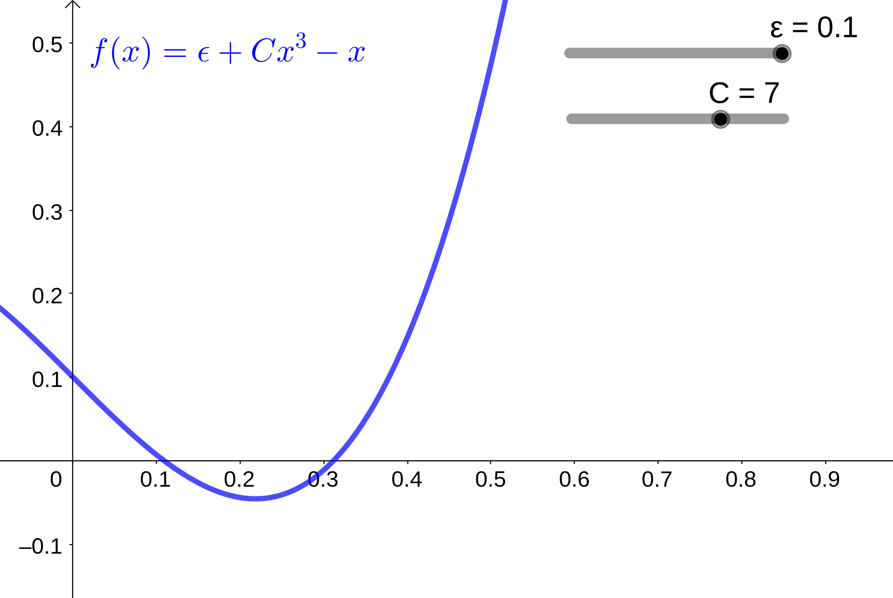
Figure 1. This graph shows the function $f:[0,\infty),f(x):=\varepsilon+Cx^{3}-x$ for $\varepsilon=0.1$ and $C=7$. Note that the set $\{f\geq 0\}$ consists of two disjoint closed intervals.

We know that $u$ is a global $H^{2}$-solution by Theorem 2.11. By Theorem 2.16, using the uniqueness of solutions, there exists a $T_{\max}\in(0,\infty]$ such that $u\in C\left([0,T_{\max}),H^{k}(\mathbb{R}^{d})\right)$. Furthermore, by Theorem 2.16, the blow-up alternative holds: If $T_{\max}<\infty$, then $\lim_{t\uparrow T_{\max}}||u||_{H^{k}}=\infty$ and $\lim_{t\uparrow T_{\max}}||u||_{\infty}=\infty$. By the Sobolev embedding theorem, the function $[0,\infty)\to[0,\infty],\ T\mapsto M(T)$ is continuous on $[0,T_{\max})$; in particular, $M(T)$ is finite on that interval.

Assume that $M(0)\leq\sup I_{1}=:C_{0}<\infty$. We claim that $T_{\max}=\infty$ and $M(T)\leq C_{0}$ for all $T\geq 0$. We have $M(T)\leq C_{0}$ for all $T\in[0,T_{\max})$ by equation (37), Lemma 3.7 and the continuity of $T\mapsto M(T)$ on $[0,T_{\max})$. If $T_{\max}<\infty$, then, by the blow-up alternative and the definition of $M(T)$, we get $\lim_{T\uparrow T_{\max}}M(T)=\infty$, which is a contradiction. Thus, $T_{\max}=\infty$ and hence, $M(T)\leq C_{0}$ for all $T\geq 0$.

1.3. Organisation

In Section 2, we recall and prove technical results, which we will need for the proof of our main result. We recall various results on solutions to the Hartree type equation from [2]. In order to be able to deal with non-zero external potentials $V$, we look at dispersive estimates for $e^{-\mathrm{i}tH}$. We recall conditions under which there is an $L^{1}$–$L^{\infty}$ dispersive estimate and we prove (33). Section 3 is devoted to proving the estimates, which we need for the proof of the main result. In Section 4, we prove Theorem 1.1. We follow the proof strategy explained in Subsection 1.2. Furthermore, we show an extension of Theorem 1.1 for large data under certain additional assumptions and we prove Theorem 1.7.

1.4. Notations

We use the convention that all constants with an upper index are greater than or equal to $1$ unless we define them otherwise. For instance, we have

$$C^{S},C^{ES},C^{V},C^{DS},C^{KP}\geq 1\,.$$ (39)

For external potentials $V:\mathbb{R}^{d}\to\mathbb{R}$, define the operator $H:=-\Delta+V$.

Acknowledgements. The author would like to express her deepest gratitude to Phan Thành Nam for his continued support and very helpful discussions. The author acknowledges the support from the Deutsche Forschungsgemeinschaft (DFG project Nr. 426365943).

2. Preliminaries

In this section, we recall some known results and we prove several technical lemmata, which we will need for our proofs.

2.1. Dispersive estimates for $e^{-\mathrm{i}tH}$

A natural question is to ask under which conditions on the external potential $V$ the operator $e^{-\mathrm{i}tH}$ satisfies a dispersive estimate similar to $e^{-\mathrm{i}t(-\Delta)}$. The proof of the following theorem under condition $(1)$ was provided in [39, Theorem 1.1] and under condition $(2)$, a proof can be found in [40, Theorem 1.1].

Theorem 2.1 (Dispersive estimate for $e^{-\mathrm{i}tH}$ in $d\geq 3$).

Let $d\geq 3$ and let $V:\mathbb{R}^{d}\to\mathbb{R}$. Furthermore, assume that one of the following assumptions is satisfied:

1. 1. There exist $\eta>0$ and $\alpha>d+4$ such that the multiplication operator $\left(1+|x|^{2}\right)^{\frac{\alpha}{2}}V(x)$ is a bounded operator from $H^{\eta}(\mathbb{R}^{d})$ to $H^{\eta}(\mathbb{R}^{d})$.

   2. $\widehat{V}\in L^{1}(\mathbb{R}^{d})$.

   3. The operator $H$ has purely absolutely continuous spectrum.

   4. $0$ is neither an eigenvalue nor a resonance for $H$. That is, there exists no function $\psi\neq 0$ in the weighted $L^{2}$-space $L^{2}(\langle x\rangle^{\sigma}\mathrm{d}x)$ for some $\sigma\geq 0$ such that $H\psi=0$ in the distributional sense.

2. $d=3$,

   $$\int_{\mathbb{R}^{3}}\mathrm{d}{x}\,\int_{\mathbb{R}^{3}}\mathrm{d}{y}\,\frac{|V(x)||V(y)|}{|x-y|^{2}}<(4\pi)^{2}$$ (40)

   and

   $$\sup_{x\in\mathbb{R}^{3}}\int_{\mathbb{R}^{3}}\mathrm{d}{y}\,\frac{|V(y)|}{|x-y|}<4\pi\,.$$ (41)

Then there exists a constant $C^{V}=C^{V}(d,V)\geq 1$ such that for all $f\in L^{1}(\mathbb{R}^{d})\cap L^{2}(\mathbb{R}^{d})$ and all $t\in\mathbb{R}\setminus\{0\}$, we have

$$||e^{-\mathrm{i}tH}f||_{\infty}\leq C^{V}\frac{1}{|t|^{\frac{d}{2}}}||f||_{1}\,.$$ (42)

More generally, if $p\in[2,\infty]$ and $\frac{1}{p}+\frac{1}{p^{\prime}}=1$, the following $L^{p}$-dispersive estimate holds true: For all $f\in L^{p^{\prime}}(\mathbb{R}^{d})\cap L^{2}(\mathbb{R}^{d})$ and all $t\in\mathbb{R}\setminus\{0\}$, we have

$$||e^{-\mathrm{i}tH}f||_{p}\leq C^{V}|t|^{-\frac{d}{2}\left(\frac{1}{p^{\prime}}-\frac{1}{p}\right)}||f||_{p^{\prime}}\,.$$ (43)

Remark 2.2.

If condition $(1)$ or $(2)$ is satisfied, then $H$ is a self-adjoint operator. In particular, $e^{-\mathrm{i}tH}$ is unitary. The $L^{p}$-dispersive estimate follows from the conservation of the $L^{2}$ norm, the dispersive estimate (42) and the Riesz-Thorin interpolation theorem, see for example [14, Theorem 2.1, Lemma 4.1]. Note that we chose $C^{V}\geq 1$ and thus, the constant does not change for $p\in[2,\infty]$.

Lemma 2.3 ($W^{k,p}(\mathbb{R}^{d})$-dispersive estimate for $e^{\mathrm{i}tH}$).

Let $d\geq 1$, $2\leq p<\infty$ and assume that $V:\mathbb{R}^{d}\to\mathbb{R}$ is such that $e^{-\mathrm{i}tH}$ is a unitary operator, which satisfies the dispersive estimate $||e^{-\mathrm{i}tH}f||_{\infty}\leq C^{V}|t|^{-\frac{d}{2}}||f||_{1}$ for some constant $C^{V}\geq 1$. Let $k\in\mathbb{N}_{0}$ be even and assume that $V\in W^{k,\infty}(\mathbb{R}^{d})$. Then there exists a constant $C^{DS}=C^{DS}(d,k,||V||_{W^{k,\infty}},C^{V})\geq 1$ such that

$$||e^{-\mathrm{i}tH}f||_{W^{k,p}}\leq C^{DS}|t|^{-\frac{d}{2}\left(\frac{1}{p^{\prime}}-\frac{1}{p}\right)}||f||_{W^{k,p^{\prime}}}$$ (44)

for all $f\in W^{k,p^{\prime}}(\mathbb{R}^{d})\cap L^{2}(\mathbb{R}^{d})$.

Remark 2.4.

• Yajima proved decay estimates of this form under various decay assumptions on $V$ and its derivatives, see [41, Theorem 1.3] and [42, Theorem 1.1, Theorem 1.2].

• Lemma 2.3 provides a simple and certainly not optimal condition, under which an $L^{1}$–$L^{\infty}$ decay estimate extends to a $W^{k,p^{\prime}}$–$W^{k,p}$ decay estimate, namely if $V\in W^{k,\infty}(\mathbb{R}^{d})$. This is sufficient for the proof of our main theorem. By contrast, the results by Yajima include the proof of an $L^{1}$–$L^{\infty}$ decay estimate, which is just a special case of the $W^{k,p^{\prime}}$–$W^{k,p}$ decay estimate, see [41, 42]. Moreover, note that Yajima proved these decay estimates for all $2\leq p\leq\infty$, whereas we had to exclude $p=\infty$ in Lemma 2.3.

• If we are only interested in the case $p=2$, we do not need the assumption that $e^{-\mathrm{i}tH}$ satisfies the dispersive estimate $||e^{-\mathrm{i}tH}f||_{\infty}\leq C^{V}|t|^{-\frac{d}{2}}||f||_{1}$. Instead, it suffices to assume that $H$ is a self-adjoint operator and hence, $e^{-\mathrm{i}tH}$ is unitary.

Proof of Lemma 2.3 for $p=2$.

The two main ingredients of the proof are the fact that $H$ and $e^{-\mathrm{i}tH}$ commute and that there exists a constant $C=C(d,k,||V||_{W^{k,\infty}})>0$ such that

$$\frac{1}{C}\sum_{j=0}^{\frac{k}{2}}||(-\Delta+V)^{j}\phi||_{2}\leq||\phi||_{H^{k}}\leq C\sum_{j=0}^{\frac{k}{2}}||(-\Delta+V)^{j}\phi||_{2}$$ (45)

for all $\phi\in H^{k}(\mathbb{R}^{d})$. Suppose (45) is true. Using that $e^{-\mathrm{i}tH}$ is unitary and that $H$ and $e^{-\mathrm{i}tH}$ commute, we get for every $f\in H^{k}(\mathbb{R}^{d})$

$$||e^{-\mathrm{i}tH}f||_{H^{k}} \leq C\sum_{j=0}^{\frac{k}{2}}||(-\Delta+V)^{j}e^{-\mathrm{i}tH}f||_{2}=C\sum_{j=0}^{\frac{k}{2}}||H^{j}e^{-\mathrm{i}tH}f||_{2}$$

$$=C\sum_{j=0}^{\frac{k}{2}}||e^{-\mathrm{i}tH}H^{j}f||_{2}\leq C\sum_{j=0}^{\frac{k}{2}}||H^{j}f||_{2}\leq C^{2}||f||_{H^{k}}\,.$$

It remains to show (45).

Lower bound

Let $\ell\in\mathbb{N}$, $m\in 2\mathbb{N}_{0}$ with $2\ell+m\leq k$. By the Leibniz rule, we get

$$\qquad||(-\Delta+V)^{\ell}\phi||_{H^{m}}=||(-\Delta+V)(-\Delta+V)^{\ell-1}\phi||_{H^{m}}$$

$$\leq||-\Delta(-\Delta+V)^{\ell-1}\phi||_{H^{m}}+||V(-\Delta+V)^{\ell-1}\phi||_{H^{m}}$$

$$\lesssim||(-\Delta+V)^{\ell-1}\phi||_{H^{m+2}}+||V||_{W^{m,\infty}}||(-\Delta+V)^{\ell-1}\phi||_{H^{m}}$$

$$\lesssim||(-\Delta+V)^{\ell-1}\phi||_{H^{m+2}}\,.$$

By iterating this process, we obtain

$$\sum_{j=0}^{\frac{k}{2}}||(-\Delta+V)^{j}\phi||_{2}\lesssim||\phi||_{H^{k}}\,.$$ (46)

Upper bound

Let $\ell\in\mathbb{N}_{0}$, $m\in 2\mathbb{N}$ with $2\ell+m\leq k$. Again, using the Leibniz rule, we obtain

$$\qquad||(-\Delta+V)^{\ell}\phi||_{H^{m}}\lesssim||(-\Delta+V)^{\ell}\phi||_{2}+||-\Delta(-\Delta+V)^{\ell}\phi||_{H^{m-2}}$$

$$\leq||(-\Delta+V)^{\ell}\phi||_{2}+||(-\Delta+V)(-\Delta+V)^{\ell}\phi||_{H^{m-2}}+||V(-\Delta+V)^{\ell}\phi||_{H^{m-2}}$$

$$\lesssim||(-\Delta+V)^{\ell}\phi||_{2}+||(-\Delta+V)^{\ell+1}\phi||_{H^{m-2}}+||V||_{W^{m-2,\infty}}||(-\Delta+V)^{\ell}\phi||_{H^{m-2}}$$

$$\lesssim||(-\Delta+V)^{\ell}\phi||_{H^{m-2}}+||(-\Delta+V)^{\ell+1}\phi||_{H^{m-2}}\,.$$

Note that $2\ell+(m-2)\leq k$ and $2(\ell+1)+(m-2)\leq k$. Therefore, we can iterate this estimate and we get

$$||\phi||_{H^{k}}\lesssim\sum_{j=0}^{\frac{k}{2}}||(-\Delta+V)^{j}\phi||_{2}\,.$$ (47)

∎

Remark 2.5.

The proof of Lemma 2.3 for $p\in(2,\infty)$ follows the same strategy. Instead of using the unitarity of $e^{-\mathrm{i}tH}$, this proof uses the $L^{p}$-dispersive estimate. Another key ingredient of the proof is the following: For $1<p<\infty$ and $k\in\mathbb{N}_{0}$ even, there exists a constant $C^{ES}=C^{ES}(d,k,p)\geq 1$ such that

$$\frac{1}{C^{ES}}\{||f||_{p}+||D^{k}f||_{p}\}\leq||f||_{W^{k,p}(\mathbb{R}^{d})}\leq C^{ES}\{||f||_{p}+||D^{k}f||_{p}\}$$ (48)

for all $f\in W^{k,p}(\mathbb{R}^{d})$, where $D^{k}:=(-\Delta)^{\frac{k}{2}}$. This inequality can be proved using the Gagliardo-Nirenberg inequality, see [14, Equation (3.14)], and the estimate

$$\left|\left|\frac{\partial^{2}f}{\partial x_{j}\partial x_{k}}\right|\right|_{p}\leq C||\Delta f||_{p}$$ (49)

for some constant $C=C(p)>0$ for all $1<p<\infty$, $j,k\in\{1,\cdots,d\}$ and all $f\in C_{c}^{2}(\mathbb{R}^{d})$, see [43, Proposition 3, p. 59].

2.2. The Hartree type equation

In this subsection, we consider the Hartree type equation

$$\begin{cases}\mathrm{i}\partial_{t}u&=(-\Delta+V)u+(w*|u|^{2})u\\ u(0)&=u_{0}\,.\end{cases}$$ (50)

We collect some results from the literature on existence, uniqueness and continuity of solutions to this equation, see the book by Cazenave [2].

Let us first recall the definition of weak and strong solutions to (50), see [2, Definition 3.1.1].

Definition 2.6 (Weak solutions and strong solutions).

Let $u_{0}\in H^{1}(\mathbb{R}^{d})$ and let $0\in I\subset\mathbb{R}$ be an interval.

• $u$ is called a weak $H^{1}$-solution to (50) if $u(0)=u_{0}$,

  $$u\in L^{\infty}\left(I,H^{1}(\mathbb{R}^{d})\right)\cap W^{1,\infty}\left(I,H^{-1}(\mathbb{R}^{d})\right)$$ (51)

  and

  $$0=-\mathrm{i}\partial_{t}u+(-\Delta+V)u+(w*|u|^{2})u\ \mathrm{in\ }H^{-1}(\mathbb{R}^{d})\mathrm{\ for\ almost\ every\ }t\in I.$$ (52)

• $u$ is called a strong $H^{1}$-solution to (50) if $u(0)=u_{0}$,

  $$u\in C\left(I,H^{1}(\mathbb{R}^{d})\right)\cap C^{1}\left(I,H^{-1}(\mathbb{R}^{d})\right)$$ (53)

  and

  $$0=-\mathrm{i}\partial_{t}u+(-\Delta+V)u+(w*|u|^{2})u\mathrm{\ in\ }H^{-1}(\mathbb{R}^{d})\mathrm{\ for\ every\ }t\in I.$$ (54)

Let us now define well-posedness for the Hartree type equation (50), see [2, Definition 3.1.5].

Definition 2.7 (Local well-posedness in $H^{1}$).

We call the initial value problem (50) locally well-posed in $H^{1}$ if the following properties hold:

• There is uniqueness in $H^{1}$ for (50), that is, for every $u_{0}\in H^{1}(\mathbb{R}^{d})$ and for every interval $0\in I\subset\mathbb{R}$, any two weak solutions to (50) on $I$ coincide.

• For every $u_{0}\in H^{1}(\mathbb{R}^{d})$, there exists a strong $H^{1}$-solution $u$ defined on a maximal interval $(-T_{\min},T_{\max})$, where $T_{\min},T_{\max}\in(0,\infty]$. $T_{\min}$ and $T_{\max}$ can depend on the initial data $u_{0}$.

• There is the blow-up alternative: If $T_{\max}<\infty$, then $\lim_{T\uparrow T_{\max}}||u(t)||_{H^{1}}=\infty$ (similarly for $T_{\min}$).

• The solution $u$ depends continuously on the initial data $u_{0}$: If $u_{0}^{n}\to u_{0}$ in $H^{1}(\mathbb{R}^{d})$ as $n\to\infty$ and $I\subset(-T_{\min},T_{\max})$ is a closed and bounded interval, then there exists $N\in\mathbb{N}$ such that for all $n\geq N$, we know that the corresponding solution to the Hartree type equation $u^{n}$ is defined on $I$. Furthermore, $u^{n}\to u$ in $C\left(I,H^{1}(\mathbb{R}^{d})\right)$ as $n\to\infty$.

Let us define the energy, see [2, Equation (3.3.9)].

Definition 2.8 (Energy).

Let $V:\mathbb{R}^{d}\to\mathbb{R}$, $V\in L^{p_{V}}(\mathbb{R}^{d})+L^{q_{V}}(\mathbb{R}^{d})$ for some $p_{V},q_{V}\geq 1$ with $p_{V},q_{V}>\frac{d}{2}$ and let $w:\mathbb{R}^{d}\to\mathbb{R}$ be an even function with $w\in L^{p_{w}}(\mathbb{R}^{d})$ for some $p_{w}\geq 1$ with $p_{w}>\frac{d}{4}$. For any $v\in H^{1}(\mathbb{R}^{d})$, we define the energy by

$$E(v):=\int_{\mathbb{R}^{d}}|\nabla v|^{2}+\int_{\mathbb{R}^{d}}\mathrm{d}{x}\,V(x)|v(x)|^{2}+\frac{1}{2}\int_{\mathbb{R}^{d}}\mathrm{d}{x}\,(w*|v|^{2})(x)|v(x)|^{2}\,.$$ (55)

Remark 2.9.

For every $v\in H^{1}(\mathbb{R}^{d})$, we have $E(v)\in\mathbb{R}$ by [2, Proposition 3.2.2(i), Proposition 3.2.9(i)]. From the proof of these statements, we also know that the energy $E(v)$ can be bounded by a constant $C<\infty$ that only depends on $||v||_{H^{1}(\mathbb{R}^{d})}$, $||V||_{L^{p_{V}}+L^{q_{V}}}$ and $||w||_{p_{w}}$. Furthermore, $C\to 0$ as $||v||_{H^{1}(\mathbb{R}^{d})}\to 0$.

The Hartree type equation (50) is locally well-posed and mass and energy are conserved, see [2, Theorem 4.3.1, Remark 3.3.4].

Theorem 2.10 (Local well-posedness and conservation of mass and energy).

Assume that $V:\mathbb{R}^{d}\to\mathbb{R}$, $V\in L^{p_{V}}(\mathbb{R}^{d})+L^{q_{V}}(\mathbb{R}^{d})$ for some $p_{V},q_{V}\geq 1$ with $p_{V},q_{V}>\frac{d}{2}$. Moreover, assume that $w:\mathbb{R}^{d}\to\mathbb{R}$ is an even function with $w\in L^{p_{w}}(\mathbb{R}^{d})$ for some $p_{w}\geq 1$ with $p_{w}>\frac{d}{4}$. Let $u_{0}\in H^{1}(\mathbb{R}^{d})$. Then the initial value problem (50) is locally well-posed in $H^{1}$. Let $u$ be the corresponding strong $H^{1}$-solution to (50). The mass and the energy are conserved:

$$||u(t)||_{2} =||u_{0}||_{2}$$ (56)

$$E(u(t)) =E(u_{0})$$ (57)

for all $t\in(-T_{\min},T_{\max})$.

Under suitable assumptions on $V$ and $w$, strong $H^{1}$-solutions are global, see [2, Corollary 6.1.2], and we have $H^{2}$ regularity, see [2, Theorem 5.3.1, Remark 5.3.3].

Theorem 2.11 (Global $H^{2}$-solutions).

Let $V:\mathbb{R}^{d}\to\mathbb{R}$ with $V\in L^{p_{V}}(\mathbb{R}^{d})+L^{q_{V}}(\mathbb{R}^{d})$, where $p_{V},q_{V}\geq 1$ and $p_{V},q_{V}>\frac{d}{2}$. Let $w:\mathbb{R}^{d}\to\mathbb{R}$ be an even function with $w\in L^{p_{w}}(\mathbb{R}^{d})$ for some $p_{w}\geq 1$ with $p_{w}>\frac{d}{4}$. Moreover, assume that $w_{-}\in L^{\infty}(\mathbb{R}^{d})+L^{q_{w}}(\mathbb{R}^{d})$ for some $q_{w}$ with $q_{w}\geq\max\left\{1,\frac{d}{2}\right\}$ if $d\neq 2$ and $q_{w}>1$ if $d=2$. Let $u_{0}\in H^{2}(\mathbb{R}^{d})$ and let $u$ be the unique global strong $H^{1}$-solution from Theorem 2.10. Then $u$ is a global solution and $u\in C\left(\mathbb{R},H^{2}(\mathbb{R}^{d})\right)$. Furthermore,

$$\sup_{t\in\mathbb{R}}||\nabla u(t)||_{2}<\infty\,.$$ (58)

Duhamel’s formula will be one of the key ingredients of our proof.

Lemma 2.12 (Duhamel’s formula).

Let $w\in L^{p_{w}}(\mathbb{R}^{d})$ for some $p_{w}\geq 1$ with $p_{w}>\frac{d}{4}$ be an even real-valued function. Let $V:\mathbb{R}^{d}\to\mathbb{R}$ belong to $L^{p_{V}}(\mathbb{R}^{d})+L^{q_{V}}(\mathbb{R}^{d})$ for $\max\left\{\frac{d}{2},2\right\}<p_{V},q_{V}\leq\infty$. Let $u_{0}\in H^{1}(\mathbb{R}^{d})$ and let $u$ be the unique strong solution to (50) given by Theorem 2.10 defined on its maximal time interval of existence $I$ with $0\in I\subset\mathbb{R}$. Then

$$u(t)=e^{-\mathrm{i}tH}u_{0}-\mathrm{i}\int_{0}^{t}\mathrm{d}{s}\,e^{-\mathrm{i}(t-s)H}(w*|u(s)|^{2})u(s)$$ (59)

for every $t\in I$.

Proof.

By [44, Theorem on p. 25], the operator $H=-\Delta+V$ is self-adjoint on $L^{2}(\mathbb{R}^{d})$ with domain $\mathcal{D}(H)=H^{2}(\mathbb{R}^{d})$. By [2, Proposition 3.2.9(i)], the map $u\mapsto(w*|u|^{2})u$ belongs to $C\left(H^{1}(\mathbb{R}^{d}),H^{-1}(\mathbb{R}^{d})\right)$. Since $u$ is a strong $H^{1}$-solution, we have $u\in C\left(I,H^{1}(\mathbb{R}^{d})\right)\cap C^{1}\left(I,H^{-1}(\mathbb{R}^{d})\right)$ by Definition 2.6. Combining these two facts, we find that $(w*|u|^{2})u\in C\left(I,H^{-1}(\mathbb{R}^{d})\right)\subset C\left(I,H^{-2}(\mathbb{R}^{d})\right)=C\left(I,(\mathcal{D}(H))^{*}\right)$. We can now conclude by [2, Remark 1.6.1(ii)]. ∎

Remark 2.13 (Duhamel’s formula for initial data at $t=1$).

If we consider the Hartree type equation with initial data at $t=1$

$$\begin{cases}\mathrm{i}\partial_{t}u&=(-\Delta+V)u+(w*|u|^{2})u\\ u(1)&=u_{1}\,,\end{cases}$$ (60)

the corresponding Duhamel’s formula is

$$u(t)=e^{-\mathrm{i}(t-1)H}u_{1}-\mathrm{i}\int_{1}^{t}\mathrm{d}{s}\,e^{-\mathrm{i}(t-s)H}(w*|u(s)|^{2})u(s)\,.$$ (61)

Remark 2.14 (Generalised Duhamel’s formula).

The nonlinearity $(w*|u|^{2})u$ in Lemma 2.12 can be replaced by a more general nonlinearity $f\in C\left(I,H^{-2}(\mathbb{R}^{d})\right)$, see [2, Remark 1.6.1(ii)].

An analogous result to the following Lemma was proved in [2, Lemma 4.10.2] for local nonlinearities $g(u)$, where $g$ is a function $g:\mathbb{C}\to\mathbb{C}$. We prove it for the non-local interaction $g(u)=(w*|u|^{2})u$ and for $g(u)=Vu$. We will need this result for the proof of Theorem 2.16.

Lemma 2.15.

Let $d\geq 1$ and let $k\in\mathbb{N}$ with $k>\frac{d}{2}$. Moreover, let $w\in L^{1}(\mathbb{R}^{d})$. For $u:\mathbb{R}^{d}\to\mathbb{C}$, let either $g(u)=Vu$ for $V\in W^{k,\infty}(\mathbb{R}^{d})$ or $g(u):=(w*|u|^{2})u$. Let $M>0$. Then there exists a constant $C(M)>0$ such that the following properties hold:

• For all $u\in H^{k}(\mathbb{R}^{d})$ with $||u||_{\infty}\leq M$, we have

  $$||g(u)||_{H^{k}}\leq C(M)||u||_{H^{k}}\,.$$ (62)

• For all $u,v\in H^{k}(\mathbb{R}^{d})$ with $||u||_{\infty},||v||_{\infty}\leq M$, we have

  $$||g(u)-g(v)||_{2}\leq C(M)||u-v||_{2}\,.$$ (63)

• For all $u,v\in H^{k}(\mathbb{R}^{d})$ with $||u||_{H^{k}(\mathbb{R}^{d})},||v||_{H^{k}(\mathbb{R}^{d})}\leq M$, we have

  $$||g(u)-g(v)||_{H^{k}}\leq C(M)||u-v||_{H^{k}}\,.$$ (64)

Proof.

The case $g(u)=Vu$. Let $u,v\in H^{k}(\mathbb{R}^{d})$. By the Leibniz rule, we have

$$||g(u)||_{H^{k}}\leq C||V||_{W^{k,\infty}}||u||_{H^{k}}$$ (65)

for a constant $C>0$ only depending on $k$ and the dimension $d$. This shows (i). Similarly, we have

$$||g(u)-g(v)||_{H^{k}}=||V(u-v)||_{H^{k}}\leq C||V||_{W^{k,\infty}}||u-v||_{H^{k}}\,,$$ (66)

so (iii) holds. Moreover, we have

$$||g(u)-g(v)||_{2}=||V(u-v)||_{2}\leq||V||_{\infty}||u-v||_{2}\,,$$ (67)

which shows (ii).

The case $g(u):=(w*|u|^{2})u$. Let $M>0$.

Proof of (i)

Let $u\in H^{k}(\mathbb{R}^{d})$ with $||u||_{\infty}\leq M$. We have

$$||g(u)||_{H^{k}}\leq C^{ES}\left(||g(u)||_{2}+||D^{k}g(u)||_{2}\right)$$ (68)

for some constant $C^{ES}\geq 1$.

For $||g(u)||_{2}$, we estimate

$$||g(u)||_{2} =||(w*|u|^{2})u||_{2}\leq||w*|u|^{2}||_{\infty}||u||_{2}\leq||w||_{1}||u||_{\infty}^{2}||u||_{2}$$

$$\leq||w||_{1}M^{2}||u||_{2}\leq||w||_{1}M^{2}||u||_{H^{k}}\,.$$

For $||D^{k}g(u)||_{2}$, we use the Kato-Ponce inequality, which states that

$$||D^{k}(fh)||_{2}\leq C^{KP}\left(||D^{k}f||_{2}||h||_{\infty}+||f||_{\infty}||D^{k}h||_{2}\right)$$ (69)

for all $f,h$ and for some fixed constant $C^{KP}\geq 1$, see [45, Theorem 1.4(2)]. We get

$$\quad||D^{k}g(u)||_{2}=||D^{k}[(w*|u|^{2})u]||_{2}$$

$$\leq C^{KP}(||D^{k}(w*|u|^{2})||_{2}||u||_{\infty}+||w*|u|^{2}||_{\infty}||D^{k}u||_{2})$$

$$\leq C^{KP}(||w*(D^{k}(u\overline{u}))||_{2}||u||_{\infty}+||w||_{1}||u||_{\infty}^{2}||D^{k}u||_{2})$$

$$\leq C^{KP}(||w||_{1}||(D^{k}(u\overline{u}))||_{2}M+||w||_{1}M^{2}||u||_{H^{k}})$$

$$\leq C^{KP}||w||_{1}M(2C^{KP}||D^{k}u||_{2}||u||_{\infty}+M||u||_{H^{k}})$$

$$\leq 3(C^{KP})^{2}||w||_{1}M^{2}||u||_{H^{k}}\,.$$

To sum up,

$$||g(u)||_{H^{k}(\mathbb{R}^{d})}\leq C^{ES}\left(||g(u)||_{2}+||D^{k}g(u)||_{2}\right)\leq 4C^{ES}(C^{KP})^{2}||w||_{1}M^{2}||u||_{H^{k}}\,.$$ (70)

Proof of (ii)

Let $u,v\in H^{k}(\mathbb{R}^{d})$ with $||u||_{\infty},||v||_{\infty}\leq M$. We have

$$||g(u)-g(v)||_{2} =||(w*|u|^{2})u-(w*|v|^{2})v||_{2}$$

$$\leq||(w*|u|^{2})(u-v)||_{2}+||(w*(|u|^{2}-|v|^{2}))v||_{2}\,.$$

We estimate the first term by

$$||(w*|u|^{2})(u-v)||_{2} \leq||w*|u|^{2}||_{\infty}||u-v||_{2}\leq||w||_{1}||u||_{\infty}^{2}||u-v||_{2}$$

$$\leq||w||_{1}M^{2}||u-v||_{2}$$

and the second term by

$$\qquad||(w*(|u|^{2}-|v|^{2}))v||_{2}\leq||w||_{1}||(|u|+|v|)(|u|-|v|)||_{2}||v||_{\infty}$$

$$\leq||w||_{1}M(||u||_{\infty}+||v||_{\infty})|||u|-|v|||_{2}\leq 2||w||_{1}M^{2}||u-v||_{2}\,.$$

Hence,

$$||g(u)-g(v)||_{2}\leq||(w*|u|^{2})(u-v)||_{2}+||(w*(|u|^{2}-|v|^{2}))v||_{2}\leq 3||w||_{1}M^{2}||u-v||_{2}\,.$$ (71)

Proof of (iii)

Let $u,v\in H^{k}(\mathbb{R}^{d})$ with $||u||_{H^{k}(\mathbb{R}^{d})},||v||_{H^{k}(\mathbb{R}^{d})}\leq M$. We have

$$||g(u)-g(v)||_{H^{k}}\leq C^{ES}\left(||g(u)-g(v)||_{2}+||D^{k}[g(u)-g(v)]||_{2}\right)$$ (72)

for some constant $C^{ES}\geq 1$. We estimated the first summand in the proof of (ii). Thus, it remains to estimate the second summand. We have

$$\quad||D^{k}[g(u)-g(v)]||_{2}=||D^{k}[(w*|u|^{2})u-(w*|v|^{2})v]||_{2}$$

$$\leq||D^{k}[(w*|u|^{2})(u-v)]||_{2}+||D^{k}[(w*(|u|^{2}-|v|^{2}))v]||_{2}\,.$$

By the Kato-Ponce inequality and the Sobolev embedding theorem ($||f||_{\infty}\leq C^{S}||f||_{H^{k}}$ for some $C^{S}\geq 1$), we get

$$\qquad||D^{k}[(w*|u|^{2})(u-v)]||_{2}$$

$$\leq C^{KP}\left(||D^{k}[w*|u|^{2}]||_{2}||u-v||_{\infty}+||w*|u|^{2}||_{\infty}||D^{k}[u-v]||_{2}\right)$$

$$\leq C^{KP}\left(||w||_{1}||D^{k}[u\overline{u}]||_{2}||u-v||_{\infty}+||w||_{1}||u||_{\infty}^{2}||u-v||_{H^{k}}\right)$$

$$\leq C^{KP}||w||_{1}\left(C^{KP}(||D^{k}u||_{2}||\overline{u}||_{\infty}+||u||_{\infty}||D^{k}\overline{u}||_{2})||u-v||_{\infty}+||u||_{\infty}^{2}||u-v||_{H^{k}}\right)$$

$$\leq 3(C^{S})^{2}(C^{KP})^{2}||w||_{1}M^{2}||u-v||_{H^{k}}\,.$$

Similarly, we obtain

$$\qquad||D^{k}[(w*(|u|^{2}-|v|^{2}))v]||_{2}$$

$$\leq C^{KP}\left(||D^{k}[w*(|u|^{2}-|v|^{2})]||_{2}||v||_{\infty}+||w*(|u|^{2}-|v|^{2})||_{\infty}||D^{k}v||_{2}\right)$$

$$\leq C^{KP}||w||_{1}\left(||D^{k}[(u-v)\overline{u}+v\overline{(u-v)}||_{2}||v||_{\infty}+||(|u|+|v|)(|u|-|v|)||_{\infty}||v||_{H^{k}}\right)$$

$$\leq C^{KP}||w||_{1}\Big{(}C^{KP}\big{(}||D^{k}[u-v]||_{2}||u||_{\infty}+||u-v||_{\infty}||D^{k}u||_{2}+||D^{k}v||_{2}||u-v||_{\infty}$$

$$\qquad+||v||_{\infty}||D^{k}[u-v]||_{2}\big{)}||v||_{\infty}+(||u||_{\infty}+||v||_{\infty})||u-v||_{\infty}||v||_{H^{k}}\Big{)}$$

$$\leq 6(C^{S})^{2}(C^{KP})^{2}||w||_{1}M^{2}||u-v||_{H^{k}}\,.$$

Combining these two estimates, we get

$$||D^{k}[g(u)-g(v)]||_{2}\leq 9(C^{S})^{2}(C^{KP})^{2}||w||_{1}M^{2}||u-v||_{H^{k}}\,.$$ (73)

∎ Finally, let us look at the existence of $H^{k}$-solutions for $k>\frac{d}{2}$ and the corresponding blow-up criterion; compare with [2, Theorem 4.10.1].

Theorem 2.16 ($H^{k}$-solutions for $k>\frac{d}{2}$).

Let $d\geq 1$ and $k>\frac{d}{2}$. Let $V:\mathbb{R}^{d}\to\mathbb{R}$ with $V\in L^{p_{V}}(\mathbb{R}^{d})+L^{q_{V}}(\mathbb{R}^{d})$, where $p_{V},q_{V}\geq 1$ and $p_{V},q_{V}>\frac{d}{2}$. Let $w:\mathbb{R}^{d}\to\mathbb{R}$ be an even function with $w\in L^{p_{w}}(\mathbb{R}^{d})$ for some $p_{w}\geq 1$ with $p_{w}>\frac{d}{4}$. Moreover, assume that $w_{-}\in L^{\infty}(\mathbb{R}^{d})+L^{q_{w}}(\mathbb{R}^{d})$ for some $q_{w}$ with $q_{w}\geq\max\left\{1,\frac{d}{2}\right\}$ if $d\neq 2$ and $q_{w}>1$ if $d=2$. Let $u_{0}\in H^{k}(\mathbb{R}^{d})$. Then there exist $T_{\min},T_{\max}\in(0,\infty]$ and a unique maximal strong solution $u\in C\left((-T_{\min},T_{\max}),H^{k}(\mathbb{R}^{d})\right)$ of (50). Moreover, the blow-up alternative holds: If $T_{\max}<\infty$, then $\lim_{t\uparrow T_{\max}}||u||_{H^{k}}=\infty$ and $\lim_{t\uparrow T_{\max}}||u||_{\infty}=\infty$ (similarly for $T_{\min}$).

Proof.

The proof of this result is provided in step 1 and step 2 of the proof of [2, Theorem 4.10.1] up to a small modification. In step 1, [2, Lemma 4.10.2] is used, which was only proved for local nonlinearities. In our case, we use Lemma 2.15 for both the interaction part $g(u)=(w*|u|^{2})u$ and for the part with the external potential $g(u)=Vu$. In step 2, Cazenave uses the uniqueness of the solution from [2, Proposition 4.2.9]. Note that alternatively, we can use the uniqueness in $H^{1}$, which follows from Theorem 2.10. ∎

Remark 2.17.

Note that the maximal existence times $T_{\min},T_{\max}$ in Theorem 2.16 do not necessarily agree with those of $H^{1}$-solutions from Theorem 2.10. In particular, a solution could be an $H^{k}$-solution defined on a bounded maximal time interval $I$ but it could be possible to extend the solution to $\mathbb{R}$ as a global $H^{1}$-solution.

3. Various estimates

For notational reasons, it is more convenient to work with the Hartree type equation with initial data at $t=1$

$$\begin{cases}\mathrm{i}\partial_{t}u&=-\Delta u+Vu+(w*|u|^{2})u\\ u(1)&=u_{1}\end{cases}$$ (74)

instead. The smallness assumption on the initial data for this equation is

$$||e^{\mathrm{i}H}u_{1}||_{1}\,,||u_{1}||_{H^{k}}\leq\varepsilon_{0}$$ (75)

and

$$||e^{\mathrm{i}H}(\partial_{t}u)(1)||_{1}\,,||(\partial_{t}u)(1)||_{H^{k}}\leq\tilde{\varepsilon}_{0}\,.$$ (76)

In the setting of the Hartree type equation with initial data at $t=1$, Theorem 1.1 states that

$$||u(t)||_{\infty}\leq C_{0}\frac{1}{|t|^{\frac{d}{2}}}$$ (77)

and

$$||\partial_{t}u(t)||_{\infty}\leq\tilde{C}_{0}\frac{1}{|t|^{\frac{d}{2}}}$$ (78)

for all $t\geq 1$.

This section is devoted to proving the estimates we need in order to prove Theorem 1.1. Suppose that the assumptions of Theorem 1.1 are satisfied. Let $T\geq 1$ and let $1\leq t\leq T$. Moreover, assume that $1\leq s\leq t$.

Definition 3.1 (Definition of $M(T)$).

Define for $T\geq 1$

$$M(T):=\sup_{1\leq t\leq T}|t|^{\frac{d}{2}}||u(t)||_{\infty}+\sup_{1\leq t\leq T}||D^{k}u(t)||_{2}+||u_{1}||_{2}\,.$$ (79)

Let us start by proving an estimate for $\sup_{1\leq t\leq T}|t|^{\frac{d}{2}}||u(t)||_{\infty}$. In particular, we will prove both a direct estimate and a Sobolev type estimate for the term $||e^{-\mathrm{i}(t-s)H}(w*|u(s)|^{2})u(s)||_{\infty}$. Define $t_{0}:=\max\{1,t-1\}$.

Lemma 3.2 (Estimate for $||e^{-\mathrm{i}(t-1)H}u_{1}||_{\infty}$).

We have

$$|t|^{\frac{d}{2}}||e^{-\mathrm{i}(t-1)H}u_{1}||_{\infty}\leq C^{V}||e^{\mathrm{i}H}u_{1}||_{1}\,.$$ (80)

Proof.

By the dispersive estimate (Theorem 2.1), we get

$$|t|^{\frac{d}{2}}||e^{-\mathrm{i}(t-1)H}u_{1}||_{\infty}=|t|^{\frac{d}{2}}||e^{-\mathrm{i}tH}e^{\mathrm{i}H}u_{1}||_{\infty}\leq C^{V}||e^{\mathrm{i}H}u_{1}||_{1}\,.$$ (81)

∎

Lemma 3.3 (Direct estimate).

We have

$$||e^{-\mathrm{i}(t-s)H}(w*|u(s)|^{2})u(s)||_{\infty}\leq C^{V}||w||_{1}M(T)^{3}|t-s|^{-\frac{d}{2}}|s|^{-\frac{d}{2}}\,.$$ (82)

Proof.

By the dispersive estimate (Theorem 2.1), Hölder’s inequality, Young’s inequality and the conservation of the $L^{2}$ norm, see Theorem 2.10, we have

$$\qquad||e^{-\mathrm{i}(t-s)H}(w*|u(s)|^{2})u(s)||_{\infty}\leq C^{V}|t-s|^{-\frac{d}{2}}||(w*|u(s)|^{2})u(s)||_{1}$$

$$\leq C^{V}|t-s|^{-\frac{d}{2}}||(w*|u(s)|^{2})||_{1}||u(s)||_{\infty}\leq C^{V}|t-s|^{-\frac{d}{2}}||w||_{1}|||u(s)|^{2}||_{1}||u(s)||_{\infty}$$

$$\leq C^{V}||w||_{1}|t-s|^{-\frac{d}{2}}||u_{1}||_{2}^{2}||u(s)||_{\infty}\leq C^{V}||w||_{1}M(T)^{3}|t-s|^{-\frac{d}{2}}|s|^{-\frac{d}{2}}\,.$$

∎

Lemma 3.4 (Sobolev type estimate).

We have

$$||e^{-\mathrm{i}(t-s)H}(w*|u(s)|^{2})u(s)||_{\infty}\leq C^{SE}||w||_{1}M(T)^{3}|s|^{-d}\,,$$ (83)

where $C^{SE}:=4C^{S}C^{DS}C^{ES}(C^{KP})^{2}$.

Proof.

By Sobolev’s inequality for $k>\frac{d}{2}$ and Lemma 2.3 for $p=2$, we have

$$\quad||e^{-\mathrm{i}(t-s)H}(w*|u(s)|^{2})u(s)||_{\infty}\leq C^{S}||e^{-\mathrm{i}(t-s)H}(w*|u(s)|^{2})u(s)||_{H^{k}}$$

$$\leq C^{S}C^{DS}||(w*|u(s)|^{2})u(s)||_{H^{k}}$$

$$\leq C^{S}C^{DS}C^{ES}\left(||(w*|u(s)|^{2})u(s)||_{2}+||D^{k}[(w*|u(s)|^{2})u(s)]||_{2}\right)$$

for some constant $C^{ES}\geq 1$.

Estimate for $||(w*|u(s)|^{2})u(s)||_{2}$.

We have

$$\qquad||(w*|u(s)|^{2})u(s)||_{2}\leq||(w*|u(s)|^{2})||_{\infty}||u(s)||_{2}$$

$$\leq||w||_{1}|||u(s)|^{2}||_{\infty}||u_{1}||_{2}\leq||w||_{1}||u(s)||_{\infty}^{2}||u_{1}||_{2}\leq||w||_{1}M(T)^{3}|s|^{-d}\,.$$

Estimate for $||D^{k}[(w*|u(s)|^{2})u(s)]||_{2}$.

We use the Kato-Ponce inequality to get

$$\quad||D^{k}[(w*|u(s)|^{2})u(s)]||_{2}$$

$$\leq C^{KP}\left(||D^{k}[w*|u(s)|^{2}]||_{2}||u(s)||_{\infty}+||w*|u(s)|^{2}||_{\infty}||D^{k}u(s)||_{2}\ \right)$$

$$\leq C^{KP}\left(||w*(D^{k}[|u(s)|^{2}])||_{2}||u(s)||_{\infty}+||w||_{1}|||u(s)|^{2}||_{\infty}||D^{k}u(s)||_{2}\ \right)$$

$$\leq C^{KP}\left(||w||_{1}||D^{k}[u(s)\overline{u(s)}]||_{2}||u(s)||_{\infty}+||w||_{1}||u(s)||_{\infty}^{2}||D^{k}u(s)||_{2}\ \right)$$

$$\leq C^{KP}\Big{(}||w||_{1}C^{KP}(||D^{k}u(s)||_{2}||\overline{u(s)}||_{\infty}||D^{k}\overline{u(s)}||_{2}||u(s)||_{\infty})||u(s)||_{\infty}$$

$$\qquad+||w||_{1}||u(s)||_{\infty}^{2}||D^{k}u(s)||_{2}\ \Big{)}$$

$$\leq 3(C^{KP})^{2}||w||_{1}||u(s)||_{\infty}^{2}||D^{k}u(s)||_{2}$$

$$\leq 3(C^{KP})^{2}||w||_{1}M(T)^{3}|s|^{-d}\,.$$

Conclusion.

We get

$$\quad||e^{-\mathrm{i}(t-s)H}(w*|u(s)|^{2})u(s)||_{\infty}$$

$$\leq C^{S}C^{DS}C^{ES}\left(||(w*|u(s)|^{2})u(s)||_{2}+||D^{k}[(w*|u(s)|^{2})u(s)]||_{2}\right)$$

$$\leq C^{S}C^{DS}C^{ES}\left(||w||_{1}M(T)^{3}|s|^{-d}+3(C^{KP})^{2}||w||_{1}M(T)^{3}|s|^{-d}\right)$$

$$\leq 4C^{S}C^{DS}C^{ES}(C^{KP})^{2}||w||_{1}M(T)^{3}|s|^{-d}$$

$$\leq C^{SE}||w||_{1}M(T)^{3}|s|^{-d}\,,$$

where we set $C^{SE}:=4C^{S}C^{DS}C^{ES}(C^{KP})^{2}$. Note that we used the fact that $C^{S},C^{DS},C^{ES},C^{KP}\geq 1$. ∎

Corollary 3.5 (Estimate for $|t|^{\frac{d}{2}}||u(t)||_{\infty}$).

We have

$$|t|^{\frac{d}{2}}||u(t)||_{\infty}\leq C^{V}||e^{\mathrm{i}H}u_{1}||_{1}+C^{\infty E}||w||_{1}M(T)^{3}\,,$$ (84)

where $C^{\infty E}:=\frac{2^{2+\frac{d}{2}}}{d-2}C^{V}+2^{\frac{d}{2}}C^{SE}$.

Proof.

By Duhamel’s formula, see Lemma 2.12, we have

$$u(t) =e^{-\mathrm{i}(t-1)H}u_{1}-\mathrm{i}\int_{1}^{t_{0}}\mathrm{d}{s}\,e^{-\mathrm{i}(t-s)H}(w*|u(s)|^{2})u(s)$$

$$\qquad-\mathrm{i}\int_{t_{0}}^{t}\mathrm{d}{s}\,e^{-\mathrm{i}(t-s)H}(w*|u(s)|^{2})u(s)\,,$$

so we obtain

$$||u(t)||_{\infty} =||e^{-\mathrm{i}(t-1)H}u_{1}||_{\infty}+\int_{1}^{t_{0}}\mathrm{d}{s}\,||e^{-\mathrm{i}(t-s)H}(w*|u(s)|^{2})u(s)||_{\infty}$$

$$\qquad+\int_{t_{0}}^{t}\mathrm{d}{s}\,||e^{-\mathrm{i}(t-s)H}(w*|u(s)|^{2})u(s)||_{\infty}\,.$$

We use Lemma 3.2 for the first term, Lemma 3.3 for the second term and Lemma 3.4 for the third term to get

$$\quad|t|^{\frac{d}{2}}||u(t)||_{\infty}\leq C^{V}||e^{\mathrm{i}H}u_{1}||_{1}+\int_{1}^{t_{0}}\mathrm{d}{s}\,C^{V}||w||_{1}M(T)^{3}|t-s|^{-\frac{d}{2}}|s|^{-\frac{d}{2}}|t|^{\frac{d}{2}}$$

$$\qquad+\int_{t_{0}}^{t}\mathrm{d}{s}\,C^{SE}||w||_{1}M(T)^{3}|s|^{-d}|t|^{\frac{d}{2}}$$

$$\leq C^{V}||e^{\mathrm{i}H}u_{1}||_{1}+||w||_{1}M(T)^{3}\left(C^{V}\int_{1}^{t_{0}}\mathrm{d}{s}\,|t-s|^{-\frac{d}{2}}|s|^{-\frac{d}{2}}|t|^{\frac{d}{2}}+C^{SE}\int_{t_{0}}^{t}\mathrm{d}{s}\,|s|^{-d}|t|^{\frac{d}{2}}\right)\,.$$

We will estimate the integral terms separately, depending on the value of $t$.

Estimate for the integrals for $t\in[1,2]$.

By definition, $t_{0}=\max\{1,t-1\}$, so we have $t_{0}=1$ in this case. Thus, the first integral is equal to zero. For the second integral, we get by $t\leq 2$ and $s\geq 1$

$$\int_{t_{0}}^{t}\mathrm{d}{s}\,|s|^{-d}|t|^{\frac{d}{2}}\leq 2^{\frac{d}{2}}\,.$$ (85)

Estimate for the integrals for $t>2$.

If $t>2$, then $t_{0}=t-1>\frac{t}{2}$. Thus, by symmetry, we can write the first integral as

$$\quad\int_{1}^{t_{0}}\mathrm{d}{s}\,|t-s|^{-\frac{d}{2}}|s|^{-\frac{d}{2}}|t|^{\frac{d}{2}}=2\int_{1}^{\frac{t}{2}}\mathrm{d}{s}\,|t-s|^{-\frac{d}{2}}|s|^{-\frac{d}{2}}|t|^{\frac{d}{2}}=2\cdot 2^{\frac{d}{2}}\int_{1}^{\frac{t}{2}}\mathrm{d}{s}\,|s|^{-\frac{d}{2}}$$

$$\leq 2^{1+\frac{d}{2}}\int_{1}^{\infty}\mathrm{d}{s}\,|s|^{-\frac{d}{2}}\leq 2^{1+\frac{d}{2}}\frac{-1}{1-\frac{d}{2}}=\frac{2^{2+\frac{d}{2}}}{d-2}\,,$$

where we used that $t-s\geq\frac{t}{2}$. For the second integral, using $s\geq 1$, $s\geq\frac{t}{2}$ and $t-t_{0}=1$, we get

$$\int_{t_{0}}^{t}\mathrm{d}{s}\,|s|^{-d}|t|^{\frac{d}{2}}\leq\int_{t_{0}}^{t}\mathrm{d}{s}\,|s|^{-\frac{d}{2}}|s|^{-\frac{d}{2}}|t|^{\frac{d}{2}}\leq 2^{\frac{d}{2}}\,.$$ (86)

Conclusion.

In both cases, we can estimate

$$\quad|t|^{\frac{d}{2}}||u(t)||_{\infty}$$

$$\leq C^{V}||e^{\mathrm{i}H}u_{1}||_{1}+||w||_{1}M(T)^{3}\left(C^{V}\int_{1}^{t_{0}}\mathrm{d}{s}\,|t-s|^{-\frac{d}{2}}|s|^{-\frac{d}{2}}|t|^{\frac{d}{2}}+C^{SE}\int_{t_{0}}^{t}\mathrm{d}{s}\,|s|^{-d}|t|^{\frac{d}{2}}\right)$$

$$\leq C^{V}||e^{\mathrm{i}H}u_{1}||_{1}+||w||_{1}M(T)^{3}\left(C^{V}\cdot\frac{2^{2+\frac{d}{2}}}{d-2}+C^{SE}\cdot 2^{\frac{d}{2}}\right)$$

$$\leq C^{V}||e^{\mathrm{i}H}u_{1}||_{1}+C^{\infty E}||w||_{1}M(T)^{3}\,,$$

where $C^{\infty E}:=\frac{2^{2+\frac{d}{2}}}{d-2}C^{V}+2^{\frac{d}{2}}C^{SE}$. ∎ Next, we prove an estimate for $\sup_{1\leq t\leq T}||D^{k}u(t)||_{2}$.

Lemma 3.6 (Estimate for $||D^{k}u(t)||_{2}$).

We have

$$||D^{k}u(t)||_{2}\leq C^{DS}||u_{1}||_{H^{k}}+C^{kE}||w||_{1}M(T)^{3}\,,$$ (87)

where $C^{kE}:=4C^{ES}C^{DS}(C^{KP})^{2}\frac{1}{d-1}$.

Proof.

By Duhamel’s formula, we have

$$u(t)=e^{-\mathrm{i}(t-1)H}u_{1}-\mathrm{i}\int_{1}^{t}\mathrm{d}{s}\,e^{-\mathrm{i}(t-s)H}(w*|u(s)|^{2})u(s)\,,$$ (88)

so by applying $D^{k}$ to both sides, we get

$$D^{k}u(t)=D^{k}e^{-\mathrm{i}(t-1)H}u_{1}-\mathrm{i}\int_{1}^{t}\mathrm{d}{s}\,D^{k}e^{-\mathrm{i}(t-s)H}(w*|u(s)|^{2})u(s)\,.$$ (89)

By Lemma 2.3 for $p=2$, we obtain

$$\quad||D^{k}u(t)||_{2}\leq||D^{k}e^{-\mathrm{i}(t-1)H}u_{1}||_{2}+\int_{1}^{t}\mathrm{d}{s}\,||D^{k}e^{-\mathrm{i}(t-s)H}(w*|u(s)|^{2})u(s)||_{2}$$

$$\leq||e^{-\mathrm{i}(t-1)H}u_{1}||_{H^{k}}+\int_{1}^{t}\mathrm{d}{s}\,||e^{-\mathrm{i}(t-s)H}(w*|u(s)|^{2})u(s)||_{H^{k}}$$

$$\leq C^{DS}\left(||u_{1}||_{H^{k}}+\int_{1}^{t}\mathrm{d}{s}\,||(w*|u(s)|^{2})u(s)||_{H^{k}}\right)$$

$$\leq C^{DS}\Bigg{(}||u_{1}||_{H^{k}}+\int_{1}^{t}\mathrm{d}{s}\,C^{ES}\left(||(w*|u(s)|^{2})u(s)||_{2}+||D^{k}[(w*|u(s)|^{2})u(s)]||_{2}\right)\Bigg{)}$$

$$\leq C^{DS}||u_{1}||_{H^{k}}+C^{ES}C^{DS}\int_{1}^{t}\mathrm{d}{s}\,\left(||(w*|u(s)|^{2})u(s)||_{2}+||D^{k}[(w*|u(s)|^{2})u(s)]||_{2}\right)$$

for a constant $C^{ES}\geq 1$. From the proof of Lemma 3.4, we know that

$$||(w*|u(s)|^{2})u(s)||_{2}\leq||w||_{1}M(T)^{3}|s|^{-d}$$ (90)

and

$$||D^{k}[(w*|u(s)|^{2})u(s)]||_{2}\leq 3(C^{KP})^{2}||w||_{1}M(T)^{3}|s|^{-d}\,.$$ (91)

Conclusion.

To sum up, we have

$$\quad||D^{k}u(t)||_{2}$$

$$\leq C^{DS}||u_{1}||_{H^{k}}+C^{ES}C^{DS}\int_{1}^{t}\mathrm{d}{s}\,\left(||(w*|u(s)|^{2})u(s)||_{2}+||D^{k}[(w*|u(s)|^{2})u(s)]||_{2}\right)$$

$$\leq C^{DS}||u_{1}||_{H^{k}}+C^{ES}C^{DS}\int_{1}^{t}\mathrm{d}{s}\,\left(||w||_{1}M(T)^{3}|s|^{-d}+3(C^{KP})^{2}||w||_{1}M(T)^{3}|s|^{-d}\right)$$

$$\leq C^{DS}||u_{1}||_{H^{k}}+4C^{ES}C^{DS}(C^{KP})^{2}||w||_{1}M(T)^{3}\int_{1}^{t}\mathrm{d}{s}\,|s|^{-d}$$

$$\leq C^{DS}||u_{1}||_{H^{k}}+4C^{ES}C^{DS}(C^{KP})^{2}\frac{1}{d-1}||w||_{1}M(T)^{3}$$

$$\leq C^{DS}||u_{1}||_{H^{k}}+C^{kE}||w||_{1}M(T)^{3}\,,$$

where we define $C^{kE}:=4C^{ES}C^{DS}(C^{KP})^{2}\frac{1}{d-1}$. ∎

Figure 1 illustrates the result of the following small technical lemma.

Lemma 3.7.

Let $C>0$. Then there exists $\varepsilon>0$ such that the function

$$f:[0,\infty)\to\mathbb{R},f(x):=\varepsilon+Cx^{3}-x$$ (92)

satisfies the following: $\{f\geq 0\}$ consists of two disjoint intervals $I_{1},I_{2}$ that have a strictly positive distance from each other, where we choose $I_{1}$ such that $0\in I_{1}$. Moreover, $I_{1}$ is bounded.

Proof.

For every $\varepsilon>0$, we have

$$f^{\prime}(x)=3Cx^{2}-1\,.$$ (93)

Thus, $f^{\prime}$ is a smooth function that is strictly increasing and it satisfies $f^{\prime}(0)=-1$ and $\lim_{x\to\infty}f^{\prime}(x)=\infty$. It follows that $f$ has at most two zeroes. Since $f(0)=\varepsilon>0$ and $\lim_{x\to\infty}f(x)=\infty$, we are done if we can show that there exists a point $\tilde{x}\in[0,\infty)$ such that $f(\tilde{x})<0$. Note that for $x\geq 0$, we have

$$-\frac{1}{2}\geq f^{\prime}(x)=3Cx^{2}-1\iff\frac{1}{2}\geq 3Cx^{2}\iff\frac{1}{6C}\geq x^{2}\iff\frac{1}{\sqrt{6C}}\geq x\,.$$ (94)

We define $\tilde{x}:=\frac{1}{\sqrt{6C}}$. Now, choose $\varepsilon>0$ such that $\varepsilon<\frac{1}{2\sqrt{6C}}$. We obtain

$$f(\tilde{x})=f(0)+\int_{0}^{\tilde{x}}\mathrm{d}{t}\,f^{\prime}(t)\leq\varepsilon+\int_{0}^{\tilde{x}}\frac{-1}{2}=\varepsilon-\frac{1}{2}\cdot\frac{1}{\sqrt{6C}}=\varepsilon-\frac{1}{2\sqrt{6C}}<0\,.$$ (95)

∎

4. Conclusion of the main theorem

In this section, we prove Theorem 1.1 using the estimates from Section 3. Furthermore, we show an extension of Theorem 1.1 for large initial data under certain additional assumptions and we explain two proof strategies for Theorem 1.7.

Proof of Theorem 1.1.

Let us work with the Hartree type equation with initial data at $t=1$. We decompose the proof into two parts. In the first part, we prove the decay estimate

$$||u(t)||_{\infty}\leq C_{0}|t|^{-\frac{d}{2}}$$ (96)

for all $t\geq 1$. In the second part, we show

$$||\partial_{t}u(t)||_{\infty}\leq\tilde{C}_{0}|t|^{-\frac{d}{2}}$$ (97)

for all $t\geq 1$.

Part 1: $||u(t)||_{\infty}\leq C_{0}|t|^{-\frac{d}{2}}$. Define

$$C:=3||w||_{1}\max\left\{C^{\infty E},C^{kE}\right\}\,.$$ (98)

By Lemma 3.7, there exists $\varepsilon>0$ small enough such that the function

$$f:[0,\infty)\to\mathbb{R},\ f(x):=\varepsilon+Cx^{3}-x$$ (99)

satisfies the following: $\{f\geq 0\}$ consists of two intervals $I_{1},I_{2}$ that have a strictly positive distance from each other and $0\in I_{1}$. Moreover, $I_{1}$ is bounded. We fix such an $\varepsilon>0$. Let $C_{0}:=\sup I_{1}>0$ be the first zero of $f$. We define

$$\varepsilon_{0}:=\frac{\min\{\varepsilon,C_{0}\}}{3C^{V}C^{DS}}\,.$$ (100)

Thus, if the assumption

$$||e^{\mathrm{i}H}u_{1}||_{1}\,,||u_{1}||_{H^{k}}\leq\varepsilon_{0}$$ (101)

is satisfied, we know by $C^{V},C^{DS}\geq 1$ that

$$C^{V}||e^{\mathrm{i}H}u_{1}||_{1}\leq\frac{\varepsilon}{3}\,,\ C^{DS}||u_{1}||_{H^{k}}\leq\frac{\varepsilon}{3}\,,\ ||u_{1}||_{2}\leq||u_{1}||_{H^{k}}\leq\frac{\varepsilon}{3}\,.$$ (102)

Moreover, we also have

$$M(1) =||u_{1}||_{\infty}+||D^{k}u_{1}||_{2}+||u_{1}||_{2}=||e^{-\mathrm{i}H}e^{\mathrm{i}H}u_{1}||_{\infty}+||D^{k}u_{1}||_{2}+||u_{1}||_{2}$$

$$\leq C^{V}1^{-\frac{d}{2}}||e^{\mathrm{i}H}u_{1}||_{1}+||u_{1}||_{H^{k}}+||u_{1}||_{2}\leq C^{V}\varepsilon_{0}+\varepsilon_{0}+\varepsilon_{0}\leq 3C^{V}\varepsilon_{0}\leq C_{0}\,.$$

Let $T\geq 1$. By Definition 3.1, Corollary 3.5 and Lemma 3.6, we have

$$M(T) =\sup_{1\leq t\leq T}|t|^{\frac{d}{2}}||u(t)||_{\infty}+\sup_{1\leq t\leq T}||D^{k}u(t)||_{2}+||u_{1}||_{2}$$

$$\leq C^{V}||e^{\mathrm{i}H}u_{1}||_{1}+C^{\infty E}||w||_{1}M(T)^{3}+C^{DS}||u_{1}||_{H^{k}}+C^{kE}||w||_{1}M(T)^{3}+||u_{1}||_{2}$$

$$\leq\frac{\varepsilon}{3}+\frac{C}{3}M(T)^{3}+\frac{\varepsilon}{3}+\frac{C}{3}M(T)^{3}+\frac{\varepsilon}{3}\leq\varepsilon+CM(T)^{3}\,.$$

Therefore,

$$\varepsilon+CM(T)^{3}-M(T)\geq 0$$ (103)

for all $T\geq 1$ with $M(T)<\infty$.

We can now conclude as we explained at the end of Subsection 1.2. By Theorem 2.16, we know that $u\in C\left([1,T_{\max}),H^{k}(\mathbb{R}^{d})\right)$ for some $T_{\max}\in(1,\infty]$. By the Sobolev embedding theorem, $T\mapsto M(T)$ is continuous on $[1,T_{\max})$. Thus, by the choice of $\varepsilon>0$ and (103), we deduce that $M(T)\leq C_{0}$ for all $T\in[1,T_{\max})$. By the blow-up alternative in Theorem 2.16, we obtain $T_{\max}=\infty$. Therefore, $M(T)\leq C_{0}$ for all $T\geq 1$. In particular,

$$||u(t)||_{\infty}\leq\frac{C_{0}}{|t|^{\frac{d}{2}}}$$ (104)

for all $t\geq 1$, which is the desired result.

Part 2: $||\partial_{t}u(t)||_{\infty}\leq\tilde{C}_{0}|t|^{-\frac{d}{2}}$. Let $\varepsilon,C,C_{0}>0$ be as in the proof of part 1. Our proof strategy is to define a quantity $\tilde{M}(T)$ similar to $M(T)$, which contains $\sup_{1\leq t\leq T}|t|^{\frac{d}{2}}||\partial_{t}u(t)||_{\infty}$. Our goal is to prove a bound of the form

$$\tilde{M}(T)\leq\tilde{\varepsilon}+\tilde{C}(\tilde{M}(T))^{3}$$ (105)

and to argue as before. It will be essential to make sure that $M(T)$ is small for all $T\geq 1$.

Boundedness of $||\partial_{t}u||_{2}$

The Hartree type equation is

$$\mathrm{i}\partial_{t}u=-\Delta u+Vu+(w*|u|^{2})u\,.$$ (106)

Thus, for every $t\geq 1$, we have

$$||\partial_{t}u(t)||_{2} \leq||\Delta u(t)||_{2}+||V||_{\infty}||u_{1}||_{2}+||w*|u(t)|^{2}||_{\infty}||u_{1}||_{2}$$

$$\leq(||D^{k}u(t)||_{2}+||u_{1}||_{2})+||V||_{\infty}||u_{1}||_{2}+||w||_{1}||u(t)||_{\infty}^{2}||u_{1}||_{2}$$

$$\leq(C_{0}+C_{0})+||V||_{\infty}C_{0}+||w||_{1}C_{0}^{3}\leq C_{0}(2+||V||_{\infty}+||w||_{1}C_{0}^{2})\,,$$

where we used $k\geq 2$, $||u(t)||_{\infty}^{2}\leq\left(C_{0}|t|^{-\frac{d}{2}}\right)^{2}\leq C_{0}^{2}$ since $t\geq 1$ and

$$||\Delta u||_{2}^{2}\leq||u||_{2}^{2}+||D^{k}u||_{2}^{2}\leq\left(||u||_{2}+||D^{k}u||_{2}\right)^{2}\,.$$ (107)

In particular, $||\partial_{t}u(t)||_{2}$ is bounded by a constant, which is small if $C_{0}$ is small.

Duhamel’s formula for $\partial_{t}u(t)$.

Differentiating the Hartree type equation with respect to time, we get

$$\mathrm{i}\partial_{t}(\partial_{t}u)=(-\Delta+V)(\partial_{t}u)+\partial_{t}[(w*|u|^{2})u]\,.$$ (108)

We can differentiate the Hartree type equation because

$$u\in C\left([1,\infty),H^{k}(\mathbb{R}^{d})\right)\cap C^{1}\left([1,\infty),H^{-1}(\mathbb{R}^{d})\right)\,.$$ (109)

Note that (108) holds for every $t\in[1,\infty)$.

We would like to apply Duhamel’s formula for $\partial_{t}u$. To this end, we need to show that $\partial_{t}u\in C\left([1,\infty),L^{2}(\mathbb{R}^{d})\right)$ and $\partial_{t}[(w*|u|^{2})u]\in C\left([1,\infty),H^{-2}(\mathbb{R}^{d})\right)$, see Remark 2.14 and [2, Remark 1.6.1(ii)].

Let us start by showing that $\partial_{t}u\in C\left([1,\infty),L^{2}(\mathbb{R}^{d})\right)$. The fact that $-\Delta u(t)+Vu(t)$ belongs to $C\left([1,\infty),L^{2}(\mathbb{R}^{d})\right)$ follows from $u\in C\left([1,\infty),H^{k}(\mathbb{R}^{d})\right)$. Lemma 2.15(ii) together with $u\in C\left([1,\infty),H^{k}(\mathbb{R}^{d})\right)$ and $\sup_{t\geq 1}||u(t)||_{\infty}<\infty$ imply that $(w*|u|^{2})u\in C\left([1,\infty),L^{2}(\mathbb{R}^{d})\right)$. Therefore, $\partial_{t}u\in C\left([1,\infty),L^{2}(\mathbb{R}^{d})\right)$ holds true because $u$ satisfies the Hartree type equation (106).

We have

$$\partial_{t}[(w*|u|^{2})u]=(w*(\overline{u}\partial_{t}u+u\overline{\partial_{t}u}))u+(w*|u|^{2})\partial_{t}u\,.$$ (110)

Now, similar to the proof of Lemma 2.15(ii), we can show that

$$\partial_{t}[(w*|u|^{2})u]\in C\left([1,\infty),L^{2}(\mathbb{R}^{d})\right)$$ (111)

using $\partial_{t}u\in C\left([1,\infty),L^{2}(\mathbb{R}^{d})\right)$ and $u\in C\left([1,\infty),H^{k}(\mathbb{R}^{d})\right)$. We omit a detailed computation here.

Therefore, we can apply Duhamel’s formula to (108) to get

$$(\partial_{t}u)(t)=e^{-\mathrm{i}(t-1)H}(\partial_{t}u)(1)-\mathrm{i}\int_{1}^{t}\mathrm{d}{s}\,e^{-\mathrm{i}(t-s)H}\partial_{t}[(w*|u|^{2})u](s)\,.$$ (112)

Definition of $\tilde{M}(T)$.

For every $T\geq 1$, define

$$\tilde{M}(T):=M(T)+\sup_{1\leq t\leq T}|t|^{\frac{d}{2}}||(\partial_{t}u)(t)||_{\infty}+\sup_{1\leq t\leq T}||D^{k}(\partial_{t}u)(t)||_{2}+\sup_{1\leq t\leq T}||(\partial_{t}u)(t)||_{2}\,.$$ (113)

Estimates for $\sup_{1\leq t\leq T}|t|^{\frac{d}{2}}||(\partial_{t}u)(t)||_{\infty}$ and $\sup_{1\leq t\leq T}||D^{k}(\partial_{t}u)(t)||_{2}$.

Using the same type of estimates as in the proof of Theorem 1.1, we can estimate

$$\sup_{1\leq t\leq T}|t|^{\frac{d}{2}}||(\partial_{t}u)(t)||_{\infty}\leq C^{V}||e^{\mathrm{i}H}(\partial_{t}u)(1)||_{1}+\frac{\tilde{C}}{3}\tilde{M}(T)^{3}$$ (114)

and

$$\sup_{1\leq t\leq T}||D^{k}(\partial_{t}u)(t)||_{2}\leq C^{DS}||(\partial_{t}u)(1)||_{H^{k}}+\frac{\tilde{C}}{3}\tilde{M}(T)^{3}$$ (115)

for some $\tilde{C}>0$, which only depends on $d,V,||w||_{1}$. Thus, if

$$\sup_{1\leq t\leq T}M(T)+\sup_{1\leq t\leq T}||(\partial_{t}u)(t)||_{2}\leq C_{0}(3+||V||_{\infty}+||w||_{1}C_{0}^{2}) \leq\frac{\tilde{\varepsilon}}{3}\,,$$

$$C^{V}||e^{\mathrm{i}H}(\partial_{t}u)(1)||_{1} \leq\frac{\tilde{\varepsilon}}{3}\,,$$

$$C^{DS}||(\partial_{t}u)(1)||_{H^{k}} \leq\frac{\tilde{\varepsilon}}{3}\,,$$

where we used $M(T)\leq C_{0}$ and the bound for $||\partial_{t}u||_{2}$, we get

$$\tilde{M}(T)\leq\tilde{\varepsilon}+\tilde{C}(\tilde{M}(T))^{3}$$ (116)

for all $T\geq 1$.

Conclusion.

Choose $\tilde{\varepsilon}>0$ small enough such that $\{\tilde{f}\geq 0\}$ consists of two disjoint closed intervals, where $\tilde{f}:[0,\infty)\to\mathbb{R},\ x\mapsto\tilde{\varepsilon}+\tilde{C}x^{3}-x$. Fix this $\tilde{\varepsilon}>0$. Now choose $\varepsilon>0$ small enough, and hence $C_{0}=C_{0}(\varepsilon,C)>0$ small enough such that $\{f\geq 0\}$ consists of two disjoint closed intervals and

$$C_{0}(3+||V||_{\infty}+||w||_{1}C_{0}^{2})\leq\frac{\tilde{\varepsilon}}{3}\,.$$ (117)

Here, we used that $C_{0}>0$ is small if $\varepsilon>0$ is small. So far, we have fixed $\varepsilon,C_{0},\tilde{\varepsilon},\tilde{C}_{0}$. Now suppose that the initial data satisfies

$$C^{V}||e^{\mathrm{i}H}u_{1}||_{1}\leq\frac{\varepsilon}{3}\,,\ C^{DS}||u_{1}||_{H^{k}}\leq\frac{\varepsilon}{3}\,,\ M(1)\leq C_{0}$$ (118)

and

$$C^{V}||e^{\mathrm{i}H}(\partial_{t}u)(1)||_{1}\leq\frac{\tilde{\varepsilon}}{3}\,,\ C^{DS}||(\partial_{t}u)(1)||_{H^{k}}\leq\frac{\tilde{\varepsilon}}{3}\,,\ \tilde{M}(1)\leq\tilde{C}_{0}\,.$$ (119)

Note that by the Sobolev embedding theorem, we have

$$||u_{1}||_{\infty}\leq C^{S}||u_{1}||_{H^{k}}$$ (120)

and similarly for $||(\partial_{t}u)(1)||_{\infty}$. Thus, $M(1)$ and $\tilde{M}(1)$ can be controlled by $||u_{1}||_{H^{k}}$ and $||(\partial_{t}u)(1)||_{H^{k}}$. In a similar way to the proof of [2, Theorem 4.10.1] and Theorem 2.16, we can show that there exists $T_{\max}\in(1,\infty]$ such that $\partial_{t}u\in C\left([1,T_{\max}),H^{k}(\mathbb{R}^{d})\right)$ and the corresponding blow-up alternative holds. We can now argue as in part 1 to obtain

$$\tilde{M}(T)\leq\tilde{C}_{0}$$ (121)

for all $T\geq 1$, which is the desired result. ∎

Remark 4.1 (Extension of Theorem 1.1 for large initial data under additional assumptions).

The proof of Theorem 1.1 shows that if, in addition, we know that

$$\sup_{t\geq 0}||D^{k}u(t)||_{\infty}<\infty$$ (122)

and

$$\lim_{t\to\infty}||u(t)||_{\infty}=0\,,$$ (123)

then we can also show the decay estimate

$$||u(t)||_{\infty}\leq\frac{C_{0}}{(1+|t|)^{\frac{d}{2}}}\ \mathrm{for\ all}\ t\geq 0$$ (124)

for large initial data. That is, we do not need any smallness condition on $||e^{-\mathrm{i}H}u_{1}||_{1}$, $||u_{1}||_{H^{k}}$. The proof which we present in this remark follows closely the proof strategy of [12, Corollary 3.4]. In certain circumstances, it might be known a priori that our additional assumptions are satisfied. For instance, this is the case in [12], see the beginning of Section 3 and Proposition 3.3 there.

Again, let us work in the setting of the Hartree type equation with initial data at $t=1$. Define

$$N(t):=\sup_{1\leq r\leq t}|r|^{\frac{d}{2}}||u(r)||_{\infty}\,.$$ (125)

By the proof of the direct estimate (Lemma 3.3), the Sobolev type estimate (Lemma 3.4) and our additional assumptions, we know that there exists a constant

$$C_{1}=C_{1}\left(d,\,C^{S},\,C^{ES},\,C^{V},\,C^{DS},\,C^{KP},\,||w||_{1},\,||u_{1}||_{2},\,\sup_{t\geq 1}||D^{k}u(t)||_{2}\right)>0$$ (126)

such that

$$||e^{-\mathrm{i}(t-s)H}(w*|u(s)|^{2})u(s)||_{\infty}\leq C_{1}|t-s|^{-\frac{d}{2}}N(s)|s|^{-\frac{d}{2}}$$ (127)

and

$$||e^{-\mathrm{i}(t-s)H}(w*|u(s)|^{2})u(s)||_{\infty}\leq C_{1}||u(s)||_{\infty}N(s)|s|^{-\frac{d}{2}}\,.$$ (128)

Combining (127) and (128), we get

$$||e^{-\mathrm{i}(t-s)H}(w*|u(s)|^{2})u(s)||_{\infty}\leq C_{1}||u(s)||_{\infty}^{\frac{1}{4}}|t-s|^{-\frac{3d}{8}}N(s)|s|^{-\frac{d}{2}}\,.$$ (129)

Note that $\frac{3d}{8}>1$ since $d\geq 3$ and define $C_{d}:=\int_{1}^{\infty}\mathrm{d}{s}\,|s|^{-\frac{3d}{8}}<\infty$. If $1\leq t\leq 2$, let $t_{1}:=t_{2}:=1$. If $t>2$, let $t_{1}:=\frac{t}{2}$ and $t_{2}:=t-1$. Thus, we always have $1\leq t_{1}\leq t_{2}\leq t$. We use (127) for $1\leq s\leq t_{1}$, (129) for $t_{1}\leq s\leq t_{2}$ and (128) for $t_{2}\leq s\leq t$ to get

$$|t|^{\frac{d}{2}}||u(t)||_{\infty}\leq|t|^{\frac{d}{2}}||e^{-\mathrm{i}(t-1)H}u_{1}||_{\infty}+|t|^{\frac{d}{2}}\int_{1}^{t_{1}}\mathrm{d}{s}\,||e^{-\mathrm{i}(t-s)H}(w*|u(s)|^{2})u(s)||_{\infty}$$

$$\qquad+|t|^{\frac{d}{2}}\int_{t_{1}}^{t_{2}}\mathrm{d}{s}\,||e^{-\mathrm{i}(t-s)H}(w*|u(s)|^{2})u(s)||_{\infty}$$

$$\qquad+|t|^{\frac{d}{2}}\int_{t_{2}}^{t}\mathrm{d}{s}\,||e^{-\mathrm{i}(t-s)H}(w*|u(s)|^{2})u(s)||_{\infty}$$

$$\leq C^{V}||e^{\mathrm{i}H}u_{1}||_{1}+C_{1}\int_{1}^{t_{1}}\mathrm{d}{s}\,|t|^{\frac{d}{2}}|t-s|^{-\frac{d}{2}}N(s)|s|^{-\frac{d}{2}}$$

$$\qquad+C_{1}\sup_{t_{1}\leq r\leq t_{2}}||u(r)||_{\infty}^{\frac{1}{4}}\int_{t_{1}}^{t_{2}}\mathrm{d}{s}\,|t-s|^{-\frac{3d}{8}}N(s)|t|^{\frac{d}{2}}|s|^{-\frac{d}{2}}$$

$$\qquad+C_{1}\sup_{t_{2}\leq r\leq t}||u(r)||_{\infty}\int_{t_{2}}^{t}\mathrm{d}{s}\,N(s)|t|^{\frac{d}{2}}|s|^{-\frac{d}{2}}$$

$$\leq C^{V}||e^{\mathrm{i}H}u_{1}||_{1}+2^{\frac{d}{2}}C_{1}\int_{1}^{t_{1}}\mathrm{d}{s}\,N(s)|s|^{-\frac{d}{2}}+2^{\frac{d}{2}}C_{1}N(t)\sup_{t_{1}\leq r\leq t}||u(r)||_{\infty}^{\frac{1}{4}}\int_{t_{1}}^{t_{2}}\mathrm{d}{s}\,|t-s|^{-\frac{3d}{8}}$$

$$\qquad+2^{\frac{d}{2}}C_{1}N(t)\sup_{t_{1}\leq r\leq t}||u(r)||_{\infty}$$

$$\leq C^{V}||e^{\mathrm{i}H}u_{1}||_{1}+2^{\frac{d}{2}}C_{1}\int_{1}^{t_{1}}\mathrm{d}{s}\,N(s)|s|^{-\frac{d}{2}}$$

$$\qquad+2^{\frac{d}{2}}C_{1}(C_{d}+1)\sup_{t_{1}\leq r\leq t}\left(||u(r)||_{\infty}^{\frac{1}{4}}+||u(r)||_{\infty}\right)N(t)\,.$$

Fix $T_{0}\geq 2$ large enough such that

$$2^{\frac{d}{2}}C_{1}(C_{d}+1)\sup_{\frac{T_{0}}{2}\leq r}\left(||u(r)||_{\infty}^{\frac{1}{4}}+||u(r)||_{\infty}\right)\leq\frac{1}{2}\,.$$ (130)

Note that this is possible because $\lim_{t\to\infty}||u(t)||_{\infty}=0$. Let $T\geq T_{0}$. By taking the supremum over $1\leq t\leq T$, we get

$$\qquad N(T)=\sup_{1\leq r\leq T}|r|^{\frac{d}{2}}||u(r)||_{\infty}\leq\sup_{1\leq r\leq T_{0}}|r|^{\frac{d}{2}}||u(r)||_{\infty}+\sup_{T_{0}\leq r\leq T}|r|^{\frac{d}{2}}||u(r)||_{\infty}$$

$$\leq N(T_{0})+C^{V}||e^{\mathrm{i}H}u_{1}||_{1}+2^{\frac{d}{2}}C_{1}\int_{1}^{T}\mathrm{d}{s}\,N(s)|s|^{-\frac{d}{2}}+\frac{1}{2}N(T)$$

$$\leq N(T_{0})+C^{V}||e^{\mathrm{i}H}u_{1}||_{1}+2^{\frac{d}{2}}C_{1}\int_{1}^{T_{0}}\mathrm{d}{s}\,N(s)|s|^{-\frac{d}{2}}+2^{\frac{d}{2}}C_{1}\int_{T_{0}}^{T}\mathrm{d}{s}\,N(s)|s|^{-\frac{d}{2}}+\frac{1}{2}N(T)$$

$$\leq N(T_{0})+C^{V}||e^{\mathrm{i}H}u_{1}||_{1}+2^{\frac{d}{2}}C_{1}\frac{1}{\frac{d}{2}-1}N(T_{0})+2^{\frac{d}{2}}C_{1}\int_{T_{0}}^{T}\mathrm{d}{s}\,N(s)|s|^{-\frac{d}{2}}+\frac{1}{2}N(T)$$

$$\leq\left(1+2^{\frac{d}{2}}C_{1}\frac{2}{d-2}\right)N(T_{0})+C^{V}||e^{\mathrm{i}H}u_{1}||_{1}+2^{\frac{d}{2}}C_{1}\int_{T_{0}}^{T}\mathrm{d}{s}\,N(s)|s|^{-\frac{d}{2}}+\frac{1}{2}N(T)\,.$$

Therefore, since $N(T)<\infty$ for every $T\geq 1$, we have

$$N(T)\leq 2\left(1+2^{\frac{d}{2}}C_{1}\frac{2}{d-2}\right)N(T_{0})+2C^{V}||e^{\mathrm{i}H}u_{1}||_{1}+2^{\frac{d}{2}+1}C_{1}\int_{T_{0}}^{T}\mathrm{d}{s}\,N(s)|s|^{-\frac{d}{2}}\,.$$ (131)

We can now apply Gronwall’s inequality, see [46, Lemma 2.7], with

$$I :=[T_{0},\infty)$$

$$\alpha :=2\left(1+2^{\frac{d}{2}}C_{1}\frac{2}{d-2}\right)N(T_{0})+2C^{V}||e^{\mathrm{i}H}u_{1}||_{1}$$

$$\beta(s) :=2^{\frac{d}{2}+1}C_{1}|s|^{-\frac{d}{2}}$$

to get

$$N(T)\leq\alpha e^{\int_{T_{0}}^{T}\mathrm{d}{s}\,\beta(s)}\leq\alpha e^{||\beta||_{L^{1}(I)}}=:C_{0}<\infty\,,$$ (132)

where we used $d\geq 3$ to deduce that $||\beta||_{L^{1}(I)}<\infty$. This shows that

$$\sup_{t\geq 1}|t|^{\frac{d}{2}}||u(t)||_{\infty}\leq C_{0}\,.$$ (133)

Proof of Theorem 1.7.

We explain two different proof strategies.

Adaptation of the proof strategy for Theorem 1.1. We can prove Theorem 1.7 in a very similar way to Theorem 1.1. We need results for the cubic nonlinear Schrödinger equation that are similar to the results we mentioned in Subsection 2.2. The preliminaries we need for the cubic nonlinear Schrödinger equation are Duhamel’s formula for both $u$ and $\partial_{t}u$, a theorem on $H^{k}$-solutions similar to Theorem 2.16 and the conservation of mass on the maximal time interval of existence of the $H^{k}$-solution $u$.

For the theorem on $H^{k}$-solutions, we argue as in the proof of Theorem 2.16: Recall that we can closely follow the proof of [2, Theorem 4.10.1(i)] but we have to make sure that the estimates in Lemma 2.15 are satisfied for our nonlinearity $Vu\pm|u|^{2}u$ and that there is uniqueness of $H^{k}$-solutions. The assumption that $g(z)=\pm|z|^{2}z$ belongs to $C^{k}(\mathbb{C},\mathbb{C})$ in the real sense and $g(0)=0$ is satisfied, so we can use [2, Lemma 4.10.2] for this part. For the term $Vu$, we use Lemma 2.15. The uniqueness follows from [2, Proposition 4.2.9] with $s=k$, $r_{j}=\rho_{j}=2$ and $q_{j}=\infty$ using that $(\infty,2)$ is an admissible pair by [2, Definition 3.2.1] and the Sobolev inequality $||f||_{\infty}\leq C^{S}||f||_{H^{k}}$. The conservation of the $L^{2}$ norm can be obtained in the same way as in [2, Theorem 4.10.1(iii)].

Duhamel’s formula holds for the $H^{k}$-solution to the cubic nonlinear Schrödinger equation by [2, Remark 1.6.1(ii)]: If $I$ is the maximal time interval of existence, then $u\in C\left(I,H^{k}(\mathbb{R}^{d})\right)\subset C\left(I,L^{2}(\mathbb{R}^{d})\right)$. Furthermore, $\pm|u|^{2}u\in C\left(I,L^{2}(\mathbb{R}^{d})\right)\subset C\left(I,H^{-2}(\mathbb{R}^{d})\right)$ and $u_{0}\in H^{k}(\mathbb{R}^{d})\subset L^{2}(\mathbb{R}^{d})$. Moreover, we can also apply Duhamel’s formula to $\partial_{t}u$: We can differentiate the right-hand side of the equation, and therefore also the left-hand side, to get

$$\mathrm{i}\partial_{t}(\partial_{t}u)=(-\Delta+V)\partial_{t}\pm\partial_{t}\left(|u|^{2}u\right)\,.$$ (134)

By the cubic nonlinear Schrödinger equation, we know that $\partial_{t}u\in C\left(I,L^{2}(\mathbb{R}^{d})\right)$ and thus, $\pm\partial_{t}\left(|u|^{2}u\right)\in C\left(I,L^{2}(\mathbb{R}^{d})\right)\subset C\left(I,H^{-2}(\mathbb{R}^{d})\right)$. Therefore, we also have Duhamel’s formula for $\partial_{t}u$.

Using these facts, we can deduce estimates that are very similar to the estimates in Section 3 since we only use the fact that $||w||_{1}<\infty$ there. For the cubic nonlinear Schrödinger equation, we can think of $w$ as $w=\pm\delta_{0}$, which formally also satisfies this property. Using the blow-up criterion from the theorem on $H^{k}$-solutions to the cubic nonlinear Schrödinger equation, we can conclude as we explained in Subsection 1.2.

Implication from Theorem 1.1 by considering the cubic nonlinear Schrödinger equation as a limit of Hartree type equations. For simplicity, let us focus on the defocusing cubic nonlinear Schrödinger equation. The proof for the focusing case works in the same way by replacing the plus sign in front of the interaction term by a minus sign. Using the theorem on $H^{k}$-solutions for the cubic nonlinear Schrödinger equation, which we explained above, we know that there exists a maximal time interval of existence $I\subset\mathbb{R}$ of the cubic nonlinear Schrödinger equation

$$\begin{cases}\mathrm{i}\partial_{t}u&=-\Delta u+Vu+|u|^{2}u\\ u(0)&=u_{0}\,.\end{cases}$$ (135)

Moreover, the solution $u$ satisfies $u\in C\left(I,H^{k}(\mathbb{R}^{d})\right)$, the $L^{2}$ norm of $u$ is conserved in time and the blow-up alternative holds. Fix $w\in C_{c}^{\infty}(\mathbb{R}^{d})$ with $w\geq 0$, $\int_{\mathbb{R}^{d}}w=1$ and define for $n\in\mathbb{N}$ the function

$$w_{n}(x):=n^{d}w(nx)\,.$$ (136)

Note that $||w_{n}||_{1}=1$ for all $n\in\mathbb{N}$ and that $w_{n}$ converges to the delta distribution in the distributional sense. For every $n\in\mathbb{N}$ let $u_{n}$ be the solution to the Hartree type equation

$$\begin{cases}\mathrm{i}\partial_{t}u_{n}&=-\Delta u_{n}+Vu_{n}+(w_{n}*|u_{n}|^{2})u_{n}\\ u_{n}(0)&=u_{0}\,.\end{cases}$$ (137)

Fix $T>0$ with $T\in I$. For every $n\in\mathbb{N}$ and every $t\in[0,T]$, we have

$$\frac{\,\mathrm{d}}{\,\mathrm{d}t}||(u-u_{n})(t)||_{2}^{2}=2\operatorname{Im}\langle u-u_{n},|u|^{2}u-(w_{n}*|u_{n}|^{2})u_{n}\rangle\,,$$ (138)

where we used that $-\Delta+V$ is self-adjoint. We omit the $t$-dependence in these computations for simplicity of notation. Let us split this term into two parts

$$\qquad\operatorname{Im}\langle u-u_{n},|u|^{2}u-(w_{n}*|u_{n}|^{2})u_{n}\rangle$$

$$=\operatorname{Im}\langle u-u_{n},\left(|u|^{2}-w_{n}*|u|^{2}\right)u\rangle+\operatorname{Im}\langle u-u_{n},\left(w_{n}*(|u|^{2}-|u_{n}|^{2})\right)u\rangle$$

$$\qquad+\operatorname{Im}\langle u-u_{n},\left(w_{n}*|u_{n}|^{2}\right)(u-u_{n})\rangle$$

$$=\operatorname{Im}\langle u-u_{n},\left(|u|^{2}-w_{n}*|u|^{2}\right)u\rangle+\operatorname{Im}\langle u-u_{n},\left(w_{n}*(|u|^{2}-|u_{n}|^{2})\right)u\rangle=:(I)+(II)\,,$$

where we used that the third term vanishes because $w_{n}*|u_{n}|^{2}$ is real-valued. We estimate both terms separately:

$$|(I)|= \left|\operatorname{Im}\langle u-u_{n},\left(|u|^{2}-w_{n}*|u|^{2}\right)u\rangle\right|=\left|\operatorname{Im}\langle-u_{n},\left(|u|^{2}-w_{n}*|u|^{2}\right)u\rangle\right|$$

$$\leq||u_{n}||_{2}|||u|^{2}-w_{n}*|u|^{2}||_{\infty}||u||_{2}=||u_{0}||_{2}^{2}|||u|^{2}-w_{n}*|u|^{2}||_{\infty}\,.$$

For fixed $t\in[0,T]$, we know that $u\in H^{k}(\mathbb{R}^{d})\subset C_{0}(\mathbb{R}^{d})$. In particular, $|u|^{2}$ is uniformly continuous, and therefore, we know that

$$\lim_{n\to\infty}|||u|^{2}-w_{n}*|u|^{2}||_{\infty}=0\,.$$ (139)

For the second term, we have

$$|(II)| =\left|\operatorname{Im}\langle u-u_{n},\left(w_{n}*(|u|^{2}-|u_{n}|^{2})\right)u\rangle\right|\leq||u-u_{n}||_{2}||w_{n}*(|u|^{2}-|u_{n}|^{2})||_{2}||u||_{\infty}$$

$$\leq||u-u_{n}||_{2}||u\overline{(u-u_{n})}+\overline{u_{n}}(u-u_{n})||_{2}||u||_{\infty}\leq||u-u_{n}||_{2}^{2}(||u||_{\infty}+||u_{n}||_{\infty})||u||_{\infty}\,.$$

Recall that by the dispersive estimate from Theorem 1.1, we have

$$||u_{n}(t)||_{\infty}\leq\frac{C_{0}}{(1+|t|)^{\frac{d}{2}}}\,,$$ (140)

where the constant $C_{0}$ is uniform in $n$ because $||w_{n}||_{1}=1$ for all $n\in\mathbb{N}$. Moreover, recall that $||u(t)||_{H^{k}}$ is bounded uniformly in $t\in[0,T]$ because $u\in C\left(I,H^{k}(\mathbb{R}^{d})\right)$. Thus, we know that there exists a constant $C=C(T)>0$ such that

$$|(II)|\leq\frac{C}{2}||u-u_{n}||_{2}^{2}\,.$$ (141)

By (138), we obtain

$$\left|\frac{\,\mathrm{d}}{\,\mathrm{d}t}||(u-u_{n})||_{2}^{2}\right|\leq 2||u_{0}||_{2}^{2}|||u|^{2}-w_{n}*|u|^{2}||_{\infty}+C||u-u_{n}||_{2}^{2}\,.$$ (142)

Therefore, using $u(0)=u_{0}=u_{n}(0)$, we obtain

$$||(u-u_{n})(t)||_{2}^{2} \leq||(u-u_{n})(0)||_{2}^{2}+\int_{0}^{t}\mathrm{d}{s}\,\left|\left(\frac{\,\mathrm{d}}{\,\mathrm{d}t}||(u-u_{n})||_{2}^{2}\right)(s)\right|$$

$$\leq 2||u_{0}||_{2}^{2}\int_{0}^{T}\mathrm{d}{s}\,|||u(s)|^{2}-w_{n}*|u(s)|^{2}||_{\infty}+C\int_{0}^{t}\mathrm{d}{s}\,||(u-u_{n})(s)||_{2}^{2}\,.$$

Define for every $n\in\mathbb{N}$

$$\varepsilon_{n}:=\varepsilon_{n}(T):=2||u_{0}||_{2}^{2}\int_{0}^{T}\mathrm{d}{s}\,|||u(s)|^{2}-w_{n}*|u(s)|^{2}||_{\infty}$$ (143)

and note that $\lim_{n\to\infty}\varepsilon_{n}=0$ by (139), where we use the dominated convergence theorem with $2\sup_{s\in[0,T]}||u(s)||_{\infty}<\infty$ as a dominating function. By Gronwall’s inequality, we get for every $t\in[0,T]$

$$||(u-u_{n})(t)||_{2}^{2}\leq\varepsilon_{n}e^{Ct}\,,$$ (144)

and therefore

$$\lim_{n\to\infty}||(u-u_{n})(t)||_{2}^{2}=0\,.$$ (145)

We get pointwise almost everywhere convergence to $u$ at least for a subsequence $(u_{n_{k}})_{k\in\mathbb{N}}$. It follows that we get the same dispersive estimate for $u$:

$$||u(t)||_{\infty}\leq\frac{C_{0}}{(1+|t|)^{\frac{d}{2}}}$$ (146)

for all $t\in[0,T]$. Now the blow-up alternative implies that $[0,\infty)\subset I$ and therefore, we get (146) for every $t\geq 0$.

The proof of the dispersive estimate for $\partial_{t}u$ follows from the pointwise almost everywhere convergence of a subsequence of $(\partial_{t}u_{n})(t)$ to $(\partial_{t}u)(t)$ for every $t\geq 0$. For the term with $-\Delta u$, we use the compact Sobolev embedding of $H^{k-2}(\mathbb{R}^{d})$ into $L^{2}_{loc}(\mathbb{R}^{d})$ for $k>2$. Thus, we need $k=4$ in dimension $d=3$ for this proof strategy. We omit the details here. ∎

References

- [1] Boris Malomed “Encyclopedia of Nonlinear Science” Routledge, 2005, pp. 639–642
- [2] Thierry Cazenave “Semilinear Schrödinger Equations” American Mathematical Society, 2003
- [3] Thierry Dauxois and Michel Peyrard “Physique des solitons” Les Ulis: EDP Sciences; Paris: CNRS Éditions, 2004
- [4] V.. Zakharov “Stability of periodic waves of finite amplitude on the surface of a deep fluid” In Journalof Applied Mechanics and Technical Physics 9.2, 1968, pp. 86–94
- [5] Martin Goldman “Strong turbulence of plasma waves” In Reviews of Modern Physics 56.4, 1984, pp. 709–735
- [6] Guido Schneider “Photonic crystals: Mathematical Analysis and Numerical Approximation”, Oberwolfach seminars Birkhäuser, 2011, pp. 127–162
- [7] A.. Davydov “Solitons, bioenergetics, and the mechanism of muscle contraction” In International Journal of Quantum Chemistry 16.1, 1979, pp. 5–17
- [8] E.. Gross “Structure of a quantized vortex in boson systems” In Nuovo Cimento 20, 1961, pp. 454–477
- [9] L.P. Pitaevskii “Vortex Lines in an Imperfect Bose Gas” In Journal of Experimental and Theoretical Physics 13.2, 1961, pp. 451–454
- [10] A.. Leggett “Bose-Einstein condensation in the alkali gases: Some fundamental concepts” In Reviews of Modern Physics 73, 2001, pp. 307–356
- [11] Y. Pomeau and S. Rica “Model of superflow with rotons” In Physical Review Letters 71.2, 1993, pp. 247–250
- [12] M. Grillakis and M. Machedon “Pair Excitations and the Mean Field Approximation of Interacting Bosons, I” In Communications in Mathematical Physics 324, 2013, pp. 601–636
- [13] Phan Thành Nam and Marcin Napiórkowski “A note on the validity of Bogoliubov correction to mean-field dynamics” In Journal de mathématiques pures et appliquées 108.5, 2017, pp. 662–688
- [14] F. Linares and G. Ponce “Introduction to Nonlinear Dispersive Equations” Springer, 2015
- [15] W. Strauss “Nonlinear scattering theory at low energy” In Journal of functional analysis 41.1, 1981, pp. 110–133
- [16] W. Strauss “Nonlinear scattering theory at low energy: Sequel” In Journal of functional analysis 43.3, 1981, pp. 281–293
- [17] J. Ginibre and G. Velo “On a class of non linear Schrödinger equations with non local interaction” In Mathematische Zeitschrift 170.2, 1980, pp. 109–136
- [18] J. Ginibre and G. Velo “Time decay of finite energy solutions of the non linear Klein-Gordon and Schrödinger equations” In Annales de l’Institut Henri Poincaré. Physique théorique 43.4, 1985, pp. 399–442
- [19] N. Hayashi and Y. Tsutsumi “Scattering theory for Hartree type equations” In Annales de l’Institut Henri Poincaré. Physique théorique, 1987
- [20] T. Cazenave and F. Weissler “Rapidly decaying solutions of the nonlinear Schrödinger equation” In Communications in Mathematical Physics 147, 1992, pp. 75–100
- [21] T. Ozawa “Long range scattering for nonlinear Schrödinger equations in one space dimension” In Communications in Mathematical Physics 139.3, 1991, pp. 479–493
- [22] J. Ginibre and T. Ozawa “Long range scattering for nonlinear Schrödinger and Hartree equations in space dimension ” In Communications in Mathematical Physics 151.3, 1993
- [23] J. Ginibre and G. Velo “Scattering Theory in the Energy Space for a Class of Hartree Equations”, https://arxiv.org/abs/math/9809183, 1998
- [24] P. Deift and X. Zhou “Long-time asymptotics for solutions of the NLS equation with initial data in a weighted Sobolev space” In Communications on Pure and Applied Mathematics 56.8, 2003, pp. 1029–1077
- [25] T. Duyckaerts, J. Holmer and S. Roudenko “Scattering for the non-radial 3D cubic nonlinear Schrödinger equation”, https://arxiv.org/abs/0710.3630, 2007
- [26] Y. Cho and T. Ozawa “Small Data Scattering of Hartree Type Fractional Schrödinger Equations in Dimension 2 and 3” In Journal of the Korean Mathematical Society 55.2, 2018
- [27] N. Hayashi and I. Naumkin “Asymptotics for Large Time of Solutions to the Nonlinear Schrödinger and Hartree Equations” In American Journal of Mathematics 120.2, 1998, pp. 369–389
- [28] J. Kato and F. Pusateri “A new proof of long range scattering for critical nonlinear Schrödinger equations”, https://arxiv.org/abs/1004.0721, 2010
- [29] Christian Brennecke, Phan Thành Nam, Marcin Napiórkowski and Benjamin Schlein “Fluctuations of N-particle quantum dynamics around the nonlinear Schrödinger equation” In Annales de l’Institut Henri Poincaré. Analyse non linéaire, 2019, pp. 1201–1235
- [30] S. Cuccagna, V. Georgiev and N. Visciglia “Decay and scattering of small solutions of pure power NLS in with and with a potential”, https://arxiv.org/abs/1209.5863, 2012
- [31] P. Germain, F. Pusateri and F. Rousset “The nonlinear Schrödinger equation with a potential” In Annales de l’Institut Henri Poincaré. Analyse non linéaire 35.6, 2018, pp. 1477–1530
- [32] I.. Naumkin “Sharp asymptotic behavior of solutions for cubic nonlinear Schrödinger equations with a potential” In Journal of Mathematical Physics 57.5, 2016
- [33] I.. Naumkin “Nonlinear Schrödinger equations with exceptional potentials” In Journal of Differential Equations 265.9, 2018, pp. 4575–4631
- [34] M. Martinez “Decay of small odd solutions for long range Schrödinger and Hartree equations in one dimension” In Nonlinearity 33.3 IOPscience, 2020, pp. 1156–1182
- [35] F. Pusateri and A. Soffer “Bilinear estimates in the presence of a large potential and a critical NLS in 3d”, https://arxiv.org/abs/2003.00312, 2020
- [36] Y. Hong “Scattering for a Nonlinear Schrödinger Equation with a Potential”, https://arxiv.org/abs/1403.3944, 2014
- [37] K. Nakanishi “Global dynamics below excited solitons for the nonlinear Schrödinger equation with a potential” In Journal of the Mathematical Society of Japan 69.4, 2017, pp. 1353–1401
- [38] Enno Lenzmann and Mathieu Lewin “Dynamical Ionization Bounds for Atoms” In Analysis and PDE 6.5 MSP, 2013, pp. 1183–1211
- [39] J.-L. Journé, A. Soffer and C. Sogge “Decay estimates for Schrödinger operators” In Communications on Pure and Applied Mathematics 44.5, 1991, pp. 573–604
- [40] I. Rodnianski and W. Schlag “Time decay for solutions of Schrödinger equations with rough and time-dependent potentials” In Interventiones Mathematicae 155.3, 2004, pp. 451–513
- [41] K. Yajima “The -continuity of wave operators for Schrödinger operators” In Journal of the Mathematical Society of Japan 47.3, 1995, pp. 551–581
- [42] K. Yajima “The -continuity of wave operators for Schrödinger operators. III, even dimensional cases ” In Journal of Mathematical Sciences (University of Tokio) 2, 1995, pp. 311–346
- [43] E. Stein “Singular Integrals and Differentiability Properties of Functions” Princeton University Press, 1970
- [44] Phan Thành Nam “Functional Analysis II Lecture Notes”, http://www.math.lmu.de/~nam/LectureNotesFA2021.pdf, 2021
- [45] A. Gulisashvili and M. Kon “Exact Smoothing Properties of Schrödinger Semigroups” In American Journal of Mathematics 118.6, 1996, pp. 1215–1248
- [46] Gerald Teschl “Ordinary Differential Equations and Dynamical Systems” American Mathematical Society, 2012