JefiGPU: Jefimenko’s Equations on GPU

Abstract

We have implemented a GPU version of the Jefimenko’s equations — JefiGPU. Given the proper distributions of the source terms $\rho$ (charge density) and $\mathbf{J}$ (current density) in the source volume, the algorithm gives the electromagnetic fields in the observational region (not necessarily overlaps the vicinity of the sources). To verify the accuracy of the GPU implementation, we have compared the obtained results with that of the theoretical ones. Our results show that the deviations of the GPU results from the theoretical ones are around 5%. Meanwhile, we have also compared the performance of the GPU implementation with a CPU version. The simulation results indicate that the GPU code is significantly faster than the CPU version. Finally, we have studied the parameter dependence of the execution time and memory consumption on one NVIDIA Tesla V100 card. Our code can be consistently coupled to RBG (Relativistic Boltzmann equations on GPUs) and many other GPU-based algorithms in physics.

PROGRAM SUMMARY/NEW VERSION PROGRAM SUMMARY

Program Title: JefiGPU
CPC Library link to program files: (to be added by Technical Editor)
Developer’s repository link: (if available)
Code Ocean capsule: (to be added by Technical Editor)
Licensing provisions(please choose one): Apache-2.0
Programming language: Python
Supplementary material:
Journal reference of previous version:*
Does the new version supersede the previous version?:*
Reasons for the new version:*
Summary of revisions:*
Nature of problem(approx. 50-250 words):Jefimenko’s equations are numerically stable with given sources $\rho$ (charge density) and $\mathbf{J}$ (current density). Providing proper sources, Jefimenko’s equations can give the electromagnetic fields without boundary conditions. However, the relevant integrations of the Jefimenko’s equations involve a 4D space-time which is both memory and time consuming. With the help of the state-of-art GPU technique, these integrations can be evaluated with acceptable accuracy and execution time. In the present work, we have implemented a GPU version of the Jefimenko’s equations and tested the accuracy and the performance of the code. Our work have demonstrated a significant improvement of the performance compared with a similar CPU implementation.
Solution method(approx. 50-250 words):The GPU code mainly deals with the implementation of the integrations in Jefimenko’s equations. Each CUDA kernel corresponds to a spatial point of $\mathbf{E}$ and $\mathbf{B}$. The integrations involving the source region and the retarded time are performed in each CUDA kernel. Ray, Numba and Cupy packages are used to manipulate the scaling of GPU allocation and evaluation.
Additional comments including restrictions and unusual features (approx. 50-250 words):

1 Introduction

Electromagnetic force, as one of the four basic interactions, plays an important role in almost all fields in nature. The governing equations of the classical electromagnetic force are the well-known Maxwell’s equations. To solve the Maxwell’s equations numerically, various algorithms including open-source[1, 2, 3] and commercial software[4, 5, 6, 7] have been designed for both general and specific usages. Among the many approaches to solve the Maxwell’s equations, the Jefimenko’s equations[8, 9], known as the general solutions of the Maxwell’s equations, are the ones that require only the spatial distribution of the source terms $\rho$ (charge density) and $\mathbf{J}$ (current density) to give the relevant electromagnetic (EM) fields.

The benefits of the Jefimenko’s equations are two folds. First, they contain two integrals of $\rho$ and $\mathbf{J}$. Combined with the continuum relation $\nabla\cdot\mathbf{J}+\partial\rho/\partial t=0$, these integrals are equivalent to the Maxwell’s equations. Integrals are much more stable than differences. Compared with the FTDT (Finite-Difference Time-Domain)[10, 11, 1] and FDFD (Finite-Difference Frequency- Domain)[12] methods, Jefimenko’s equations do not have the trouble of numerical blow up (this is only true when we use the concept of charge screening[13]). Second, the Jefimenko’s equations do not need the boundary conditions — as long as one provides the proper distributions of the sources. The $\mathbf{E}$ and $\mathbf{B}$ fields can be obtained by performing an integration in the vicinity of the sources. This is convenient especially when we calculate the EM fields in a fixed box, since in FEM (Finite Element Method)[14, 15, 16], FDTD and FDFD one has to carefully design the boundary conditions[17, 18, 19] to absorb the reflections of the EM fields.

However, the Jefimenko’s equations also encounter certain difficulties. The integral is performed over the entire source volume space with retarded time. This requires all the information of the sources in the relevant space-time, and is therefore memory demanding. Meanwhile, the denominator of the integrated involves a divergence at $\mathbf{r}=\mathbf{r}^{\prime}$ (see Esq. (1) ~ 3). The divergence is somewhat troublesome in numerical evaluations. Thus, the refinement’s equations are usually used to solve far-field EM fields[20, 21]. Except for the numerical difficulties, the source term $\rho$ may not be easily available since it is experimentally hard to measure the charge density distributions[22]. To provide a distribution of the charge and current densities, one may need to solve the transport equations (e.g., the Boltzmann equation [23]) which is another challenge so far.

In this regard, we have applied the Jefimenko’s equation on the state-of-art GPU based on our previous work ZMCintegral[24, 25] and RBG[23]. Our present code mainly contributes to the field of Heavy-Ion collisions[26, 27, 28, 29] where the electromagnetic fields in the early time significantly influence the evolution of the quark-gluon matter. Our hope is to combine the Jefimenko’s equations to the relativistic Boltzmann equation[23] and eventually answer the question of “early thermalization”[30, 31, 32]. Due to the high clock rate, high instruction per cycle[33], and multiple cores of the GPUs, more and more numerical algorithms that were hard in the past are now possible[24, 34]. In the present work, we use the Python package Ray[35], Numba[36] and Cupy[37] to perform the jefimenko’s equations on GPU. Our work has demonstrated significant performance improvement compared with the usual CPU implementation. The results are stable and within an acceptable margin of error.

The paper is organized in the following structure. In Sec. 2, we introduce the expressions of the Jefimenko’s equations and the details of the GPU implementation. In Sec. 3, we compare the GPU results with the theoretical results. The corresponding execution time of the GPU code is also compared with a similar CPU implementation. In Sec. 4, we have investigated the parameter dependence of the GPU code on one Tesla V100 card, and presented the time consumption of HToD (Host To Device), DToH (Device To Host) and the evaluation. The conclusion and outlook of JefiGPU is in Sec. 5. Through out the paper we use the Rationalized-Lorentz-Heaviside-QCD unit.

2 GPU Implementation

2.1 Jefimenko’s equations

The Jefimenko’s equation can be directly derived from the retarded potential solution of Maxwell’s equations[22]. In Rationalized-Lorentz-Heaviside-QCD unit, the Jefimenko’s equations take the following form

$$\mathbf{E}(\mathbf{r},t) = \frac{1}{4\pi}\int\left[\frac{\mathbf{r}-\mathbf{r}^{\prime}}{|\mathbf{r}-\mathbf{r}^{\prime}|^{3}}\rho(\mathbf{r}^{\prime},t_{r})\right.$$ (1)

$$+\frac{\mathbf{r}-\mathbf{r}^{\prime}}{|\mathbf{r}-\mathbf{r}^{\prime}|^{2}}\frac{\partial\rho(\mathbf{r}^{\prime},t_{r})}{\partial t}$$

$$\left.-\frac{1}{|\mathbf{r}-\mathbf{r}^{\prime}|}\frac{\partial\mathbf{J}(\mathbf{r}^{\prime},t_{r})}{\partial t}\right]d^{3}\mathbf{r}^{\prime}$$

$$\mathbf{B}(\mathbf{r},t) = -\frac{1}{4\pi}\int\left[\frac{\mathbf{r}-\mathbf{r}^{\prime}}{|\mathbf{r}-\mathbf{r}^{\prime}|^{3}}\times\mathbf{J}(\mathbf{r}^{\prime},t_{r})\right.$$ (2)

$$+\left.\frac{\mathbf{r}-\mathbf{r}^{\prime}}{|\mathbf{r}-\mathbf{r}^{\prime}|^{2}}\times\frac{\partial\mathbf{J}(\mathbf{r}^{\prime},t_{r})}{\partial t}\right]d^{3}\mathbf{r}^{\prime}$$

$$t_{r} = t-|\mathbf{r}-\mathbf{r}^{\prime}|,$$ (3)

where $\mathbf{E}$ and $\mathbf{B}$ are the electric and magnetic field at space-time point $(\mathbf{r},t)$, $\rho$ and $\mathbf{J}$ are the charge and current densities, and $t_{r}$ is the retarded time. Once the space-time distributions of $\rho$ and $\mathbf{J}$ are given, one can use Eqs. (1) ~ 3 to obtain the field distributions in space-time.

The numerical difficulties of the Jefimenko’s equations lie in the following two aspects. First, to obtain the numerical value of $\mathbf{E}$ and $\mathbf{B}$ at each point in the observational region (not necessarily overlaps the source region), an integration involving a 4-Dimensional (4D) space-time is required. Supposing the observational region has $n_{x,\text{o}}\times n_{y,\text{o}}\times n_{z,\text{o}}=100^{3}\sim 10^{6}$ points, we need to perform $10^{6}$ integrations at each time step. If each integration involves a summation of $n_{x,\text{s}}\times n_{y,\text{s}}\times n_{z,\text{s}}=100^{3}\sim 10^{6}$ points, the task will be both time and memory consuming. Second, Jefimenko’s equations encounter a divergence at $\mathbf{r}=\mathbf{r}^{\prime}$ when the observational region overlaps the source region. The near-source divergence has its profound physical origins and the usual treatment is to adopt the concept of coarse screening[13], which is constrained by the grid size. With coarse screening, the $\mathbf{E}$ and $\mathbf{B}$ fields in a specific grid can only be generated by the charge and density sources from other grids. If one is working in the far-field calculations, then the divergence will not be a problem.

2.2 GPU implementation of Jefimenko’s equations

We define two spatial regions of sizes $n_{x,\text{s}}\times n_{y,\text{s}}\times n_{z,\text{s}}$ and $n_{x,\text{o}}\times n_{y,\text{o}}\times n_{z,\text{o}}$, where the subscripts o and s denote the physical quantities in the source and observational regions, receptively. The infinitesimal differences in these two regions are denoted as $dx_{\text{s}}\times dy_{\text{s}}\times dz_{\text{s}}$ and $dx_{\text{o}}\times dy_{\text{o}}\times dz_{\text{o}}$. In the current work, we only use one NVIDIA V100 card to test the code, and the functionality of multi-GPU on clusters is also supported via the Ray package.

For numerical convenience, we discretize Eqs. (1) ~ 3 as

$$\mathbf{E}(\mathbf{r},t) = \frac{1}{4\pi}\Sigma_{i,j,k}\left[\frac{\mathbf{r}-\mathbf{r}_{i,j,k}^{\prime}}{|\mathbf{r}-\mathbf{r}_{i,j,k}^{\prime}|^{3}}\rho(\mathbf{r}_{i,j,k}^{\prime},t_{r})\right.$$ (4)

$$+\frac{\mathbf{r}-\mathbf{r}_{i,j,k}^{\prime}}{|\mathbf{r}-\mathbf{r}_{i,j,k}^{\prime}|^{2}}\frac{\rho(\mathbf{r}_{i,j,k}^{\prime},t_{r})-\rho(\mathbf{r}_{i,j,k}^{\prime},t_{r}-dt)}{dt}$$

$$\left.-\frac{1}{|\mathbf{r}-\mathbf{r}_{i,j,k}^{\prime}|}\frac{\mathbf{J}(\mathbf{r}_{i,j,k}^{\prime},t_{r})-\mathbf{J}(\mathbf{r}_{i,j,k}^{\prime},t_{r}-dt)}{dt}\right]d\Omega^{\prime}$$

$$\mathbf{B}(\mathbf{r},t) = -\frac{1}{4\pi}\Sigma_{i,j,k}\left[\frac{\mathbf{r}-\mathbf{r}_{i,j,k}^{\prime}}{|\mathbf{r}-\mathbf{r}_{i,j,k}^{\prime}|^{3}}\times\mathbf{J}(\mathbf{r}_{i,j,k}^{\prime},t_{r})\right.$$ (5)

$$+\left.\frac{\mathbf{r}-\mathbf{r}_{i,j,k}^{\prime}}{|\mathbf{r}-\mathbf{r}_{i,j,k}^{\prime}|^{2}}\times\frac{\mathbf{J}(\mathbf{r}_{i,j,k}^{\prime},t_{r})-\mathbf{J}(\mathbf{r}_{i,j,k}^{\prime},t_{r}-dt)}{dt}\right]d\Omega^{\prime}$$

$$t_{r} = t-|\mathbf{r}-\mathbf{r}_{i,j,k}^{\prime}|,$$ (6)

where index $i\in\{1,2,...,n_{x}\}$, $j\in\{1,2,...,n_{y}\}$, $k\in\{1,2,...,n_{z}\}$ and volume element $d\Omega^{\prime}=dx^{\prime}dy^{\prime}dz^{\prime}$.

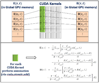
Figure 1: Schematic of the GPU implementation of Jefimenko’s equations. Each CUDA kernel corresponds to the evaluations of $\mathbf{E}(\mathbf{r}_{i},t)$ and $\mathbf{B}(\mathbf{r}_{i},t)$ at space-time point $(\mathbf{r}_{i},t)$ where $i$ is the index of the spatial grid. The integration at point $(\mathbf{r}_{i},t)$ is performed in each CUDA kernel via Eqs. (4) ~ (6).

The single GPU implementation is illustrated in Fig. 1. In each CUDA kernel we perform an integration to obtain $\mathbf{E}(\mathbf{r}_{i},t)$ and $\mathbf{B}(\mathbf{r}_{i},t)$ at space-time point $(\mathbf{r}_{i},t)$ where $i$ is the index of the spatial grid. At each call of the integration method (jargon in Python) we claim an empty space for $\mathbf{E}(\mathbf{r},t)$ and $\mathbf{B}(\mathbf{r},t)$ in the global GPU memory. The calculated EM fields via Eqs (4) ~ (6) will be stored in this empty space. After the evaluation of the integral (i.e., summation of Eqs. (4) ~ (6)), new values of $\mathbf{E}(\mathbf{r},t)$ and $\mathbf{B}(\mathbf{r},t)$ at time snapshot $t$ will be obtained (i.e., stored in the pre-allocated empty space) and transferred to the host memory. Since $\mathbf{E}(\mathbf{r},t)$ and $\mathbf{B}(\mathbf{r},t)$ are frequently transferred to the host at each time, we store them in the global GPU memory for fast data transferring. The numerical integration of Eqs. (4) ~ (6) in each CUDA kernel requires a full access of $\rho(\mathbf{r}^{\prime},t_{r})$ and $\mathbf{J}(\mathbf{r}^{\prime},t_{r})$ at all relevant space-time points (see Sec. 4 for details), thus $\rho$ and $\mathbf{J}$ should be stored in the global GPU memory. Meanwhile, the GPU memory corresponds to $\rho$ and $\mathbf{J}$ will not be released after each call of the integration method. Other temporary variables such as $\mathbf{r}^{\prime}$ and $t_{r}$ are defined in local GPU memories.

The scaling of JefiGPU on GPU clusters is straight forward — the Ray package provides a succinct API to manipulate multiple GPU cards and cluster nodes. There are three approaches to conduct the GPU scaling, as is illustrated in Fig. 2. We can divide the regions into several rectangular regions of S-O (Source region and Observational region) pairs. Each pair can be performed on one GPU card. In the code, we provide the users with a Python API to manipulate these procedures.

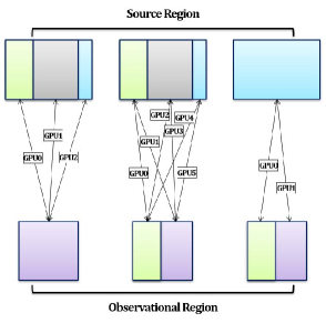
Figure 2: Three approaches for GPU scaling. The source and observational regions are divided into several sub-regions. The sub-regions will form many S-O pairs. Each S-O pair can be performed on one GPU card using the algorithm illustrated in Fig. 1.

3 Comparisons with the theoretical results and the CPU based algorithm

To see the performance of the GPU based algorithm, we will compare it with the corresponding CPU implementation. The hardware set-up of the two cases are summarized in Tab. 1. The CPU code is performed via Python with the similar algorithm stated in Fig. 1. The theoretical results are obtained in Mathematica with the built-in function NIntegrate using the GlobalAdaptive method. To avoid near-source divergence in the numerical integrations of Eqs. (1) ~ 3 in NIntegrate, we introduce a screening volume of size $\delta^{3}$. Thus both $\rho$ and $\mathbf{J}$ give zero contribution to $\mathbf{E}$ and $\mathbf{B}$ when $|i-i^{\prime}|\leq\delta$, where $i\in\{x,y,z\}$.

Table 1: Hardware set-up of the two conditions.

	Hardware of CPU	Hardware of GPU
GPU	Intel(R) Xeon(R) Silver 4110	NVIDIA Tesla V100
Implementation	CPU@2.10 GHz with 32 cores	with 32Gb memory
CPU	Intel(R) Xeon(R) Silver 4110	None
Implementation	CPU@2.10 GHz with 1 core

3.1 Constant sources

We will firstly use the constant sources to see whether the GPU-Code gives stable and acceptable results, and then compare the execution time of the GPU-Code to the CPU-Code. The sources of $\rho$ and $\mathbf{J}$ take the following form

$$\rho(x,y,z,t) = \begin{cases}0&\text{if }t<0\\ 1&\text{if }t\geq 0\end{cases}$$

$$\mathbf{J}(x,y,z,t) = \begin{cases}\mathbf{0}&\text{if }t<0\\ \mathbf{1}&\text{if }t\geq 0\end{cases},$$ (7)

where $\mathbf{0}=(0,0,0)$ and $\mathbf{1}=(1,1,1)$.

Figs. 3~5 show the results of the obtained electric and magnetic fields in the XOY plane. The integration domain (also the domain of the observational region) is of size $[-3\text{ GeV}^{-1},3\text{$\text{ GeV}^{-1}$}]^{3}$. The theoretical results are obtained via NIntegrate in Mathematica with screening length $\delta=0.2\text{ $\text{ GeV}^{-1}$}$, which is half the grid length in the GPU-Code. In the GPU implementation we have chosen $n_{x,\text{s}}=n_{y,\text{s}}=n_{z,\text{s}}=n_{x,\text{o}}=n_{y,\text{o}}=n_{z,\text{o}}=15$ such that each 3D grid is of volume size $(0.4\text{ $\text{ GeV}^{-1}$})^{3}$ .

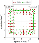
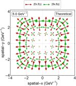
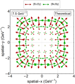
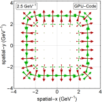
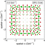
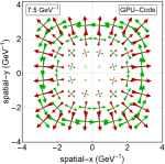
Figure 3: Electric and magnetic field in the XOY plane with constant $\rho$ and $\mathbf{J}$. The upper panel gives the theoretical results via Mathematica with built-in function NIntegrate, while the lower panel gives the results obtained by the GPU code.

Fig. 3 compares $\mathbf{E}$ and $\mathbf{B}$ at time snapshots 2.5 $\text{GeV}^{-1}$, 5 $\text{GeV}^{-1}$ and 7.5 $\text{GeV}^{-1}$. The upper panel shows the theoretical results with screening volume $\delta^{3}=(0.2\text{ $\text{GeV}^{-1}$})^{3}$, and the lower panel gives the GPU results. We can see that the two results follow the similar patterns at all time snapshots. Since the sources are constant, we expect a saturation of $\mathbf{E}$ and $\mathbf{B}$ at later times (e.g., when $t\geq 5\text{$\text{ GeV}^{-1}$}$ the fields remain almost unchanged). The near saturation at around 5 $\text{GeV}^{-1}$ is reasonable since the longest transmission length of the field is $6\text{ $\text{GeV}^{-1}$}\times\sqrt[3]{3}\sim 8.7\text{$\text{ GeV}^{-1}$}$,. Thus the system must reach a constant field distribution after $8.7\text{$\text{ GeV}^{-1}$}$.

Fig. 4 and 5 give the comparison of $|\mathbf{E}_{\text{Theo}}-\mathbf{E}_{\text{GPU}}|$ with $|\mathbf{E}_{\text{Theo}}|$ and $|\mathbf{B}_{\text{Theo}}-\mathbf{B}_{\text{GPU}}|$ with $|\mathbf{B}_{\text{Theo}}|$. In the XOY plane, the norms are taken as

$$|\mathbf{E}_{\text{Theo}}-\mathbf{E}_{\text{GPU}}| = \left[(E_{x,\text{Theo}}-E_{x,\text{GPU}})^{2}\right.$$

$$+\left.(E_{y,\text{Theo}}-E_{y,\text{GPU}})^{2}\right]^{1/2}$$

$$|\mathbf{E}_{\text{Theo}}| = \sqrt{E_{x,\text{Theo}}^{2}+E_{y,\text{Theo}}^{2}}$$

$$|\mathbf{B}_{\text{Theo}}-\mathbf{B}_{\text{GPU}}| = \left[(B_{x,\text{Theo}}-B_{x,\text{GPU}})^{2}\right.$$

$$+\left.(B_{y,\text{Theo}}-B_{y,\text{GPU}})^{2}\right]^{1/2}$$

$$|\mathbf{B}_{\text{Theo}}| = \sqrt{B_{x,\text{Theo}}^{2}+B_{y,\text{Theo}}^{2}},$$ (8)

where we neglect the $z-$component of the fields for numerical convenience. From the legend bars in Fig. 4 and 5, we can see that the maximum deviation of the GPU-Code from the theoretical results is within $0.015/0.5\sim 3$ for both $\mathbf{E}$ and $\mathbf{B}$.

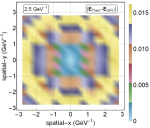
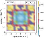
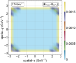
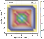
Figure 4: Norm of $\mathbf{E}_{\text{Theo}}-\mathbf{E}_{\text{GPU}}$ and $\mathbf{E}_{\text{Theo}}$ with constant sources. The norm of the two vectors are defined in the XOY plane, i.e., $|\mathbf{A}|\equiv\sqrt{A_{x}^{2}+A_{y}^{2}}$.

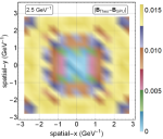
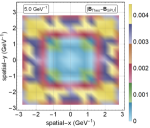
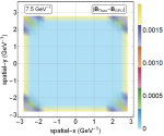
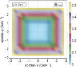
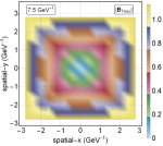
Figure 5: Norm of $\mathbf{B}_{\text{Theo}}-\mathbf{B}_{\text{GPU}}$ and $\mathbf{B}_{\text{Theo}}$ with constant sources.

3.2 Sinusoidal sources

In the sinusoidal case, we choose two different domains for the observational ($[-3\text{ GeV}^{-1},3\text{$\text{ GeV}^{-1}$}]^{2}\times[10\text{ GeV}^{-1},16\text{ GeV}^{-1}]$, where $[10\text{ GeV}^{-1},16\text{ GeV}^{-1}]$ is the interval in $z$ direction) and source regions ($[-3\text{ GeV}^{-1},3\text{$\text{ GeV}^{-1}$}]^{3}$). The sources of sinusoidal $\rho$ and $\mathbf{J}$ take the following form

$$\rho(x,y,z,t) = \begin{cases}0&\text{if }t<0\\ 3(\text{cos}(t)-1)\text{cos}(x+y+z)&\text{if }t\geq 0\end{cases}$$

$$\mathbf{J}(x,y,z,t) = \begin{cases}\mathbf{0}&\text{if }t<0\\ (j_{x},j_{y},j_{z})&\text{if }t\geq 0\end{cases},$$ (9)

where $j_{x}=j_{y}=j_{z}=\text{sin}(x+y+z)\text{sin}(t)$. Eq. (9) satisfies the continuum relation $\nabla\cdot\mathbf{J}+\partial\rho/\partial t=0$.

Fig. 6 confirms that the patterns of the EM fields obtained from the theoretical and the GPU code are similar. Different from the case of the constant sources, there is no saturation of the EM fields. Instead, we find the periodic features of the EM fields which are consistent with the sinusoidal sources. Fig. 7 and 8 show a maximum deviation from the theoretical results of $0.004/0.035\sim 11.2$ for $\mathbf{E}$ and $0.005/0.035\sim 14.3$ for $\mathbf{B}$, respectively.

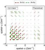
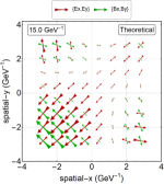
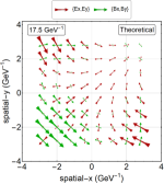
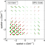
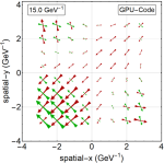
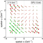
Figure 6: Electric and magnetic field in the XOY plane with sinusoidal $\rho$ and $\mathbf{J}$.

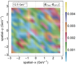
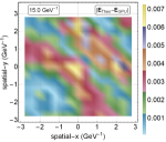
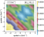
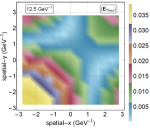
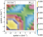
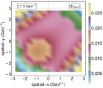
Figure 7: Norm of $\mathbf{E}_{\text{Theo}}-\mathbf{E}_{\text{GPU}}$ and $\mathbf{E}_{\text{Theo}}$ with sinusoidal sources.

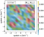
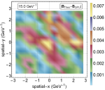
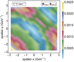
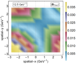
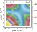
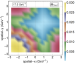
Figure 8: Norm of $\mathbf{B}_{\text{Theo}}-\mathbf{B}_{\text{GPU}}$ and $\mathbf{B}_{\text{Theo}}$ with sinusoidal sources.

3.3 Comparison of the execution time

For a comparison of the execution time, we have performed a similar algorithm depicted in Fig. 1 on a CPU apparatus whose hardware set-up is listed in Tab. 1. We have chosen the same condition as in Sec. 3.1. Tab. 2 shows the execution time of both the CPU and GPU implementations. One can see that the use of GPU can significantly enhance the performance by a factor of up to a thousand. The detailed time consumption of HToD (Host to Device) and DToH (Device to Host) will be demonstrated in Sec. 4.

Table 2: Comparison of the Execution time in GPU and CPU implementations. To save time, the CPU code only evaluates the EM field for one time-step, while the GPU code runs for totally 410 time snapshots ranging from 0 $\text{GeV}^{-1}$ to 20.5 $\text{GeV}^{-1}$. The two time-info in the table correspond to the constant/sinusoidal sources (e.g., 8.696/8.111 s means that 8.696 s is the execution time for the constant source and 8.111 s for the sinusoidal source).The last row gives the effective execution time where both implementations are assumed to be executed for the same time snapshots.

Apparatus	GPU	CPU
Execution time	8.696/8.111 s	18.012/18.540 s
Evaluated time snapshots	410	1
Effective execution time	8.696/8.111 s	2.051/2.112 h

4 Parameter dependence of the algorithm on one Tesla V100 card

There are two parameters that mainly affect the performance of the algorithm, i.e., “lts” short for length_of_time_snapshots and “ntg” short for number_of_total_grids. In Eqs. (4) ~ (6), the summations of the source terms $\rho$ and $\mathbf{J}$ are at the retarded time $t_{r}$. Therefore we need to store $\rho$ and $\mathbf{J}$ in the GPU memory at all relevant times, i.e., $\rho_{\text{GPU}}\mapsto[\rho_{0}(\mathbf{r}),\rho_{1}(\mathbf{r}),\cdots\rho_{\text{lts}}(\mathbf{r})]$ and $\mathbf{J}_{\text{GPU}}\mapsto[\mathbf{J}_{0}(\mathbf{r}),\mathbf{J}_{1}(\mathbf{r}),\cdots\mathbf{J}_{\text{lts}}(\mathbf{r})]$. If the maximum distance between the source point $\mathbf{r}_{\text{s}}$ and the observational point $\mathbf{r}_{\text{o}}$is $d_{\text{m}}=\text{max}\{|\mathbf{r}_{\text{s}}-\mathbf{r}_{\text{o}}|\}$, and the time step used in the calculation is $dt$, then we can determine the value of length_of_time_snapshots by $\text{\textquotedblleft lts\textquotedblright}=\left\lceil d_{\text{m}}/dt\right\rceil$. number_of_total_grids counts the total grid sizes of both the observational and source region, and is determined by the pair $\text{ \textquotedblleft ntg\textquotedblright}=[n_{x,\text{s}}\times n_{y,\text{s}}\times n_{z,\text{s}},n_{x,\text{o}}\times n_{y,\text{o}}\times n_{z,\text{o}}]$. The total amount of float numbers on one GPU card can be evaluated approximately as

$$N = (\left\lceil d_{\text{m}}/dt\right\rceil+1)\times n_{x,\text{s}}\times n_{y,\text{s}}\times n_{z,\text{s}}\times 4$$ (10)

$$+n_{x,\text{o}}\times n_{y,\text{o}}\times n_{z,\text{o}}\times 6,$$

where number “4” corresponds to $\rho,J_{x},J_{y},J_{z}$ and number “6” corresponds to $E_{x},E_{y},E_{z},B_{x},B_{y},B_{z}$. We can use $N$ to evaluate the occupied GPU memory in the execution. Apart from the memory consumption, the execution time is mainly constrained by “ntg” since the summation and loop are on the spatial grids.

Table 3: Occupied GPU memory at various “ntg” and “lts”.

	“ntg”	$[160^{3},160^{3}]$	$[100^{3},100^{3}]$	$[70^{3},70^{3}]$	$[60^{3},60^{3}]$	$[20^{3},20^{3}]$
“lts”
9000					30025MiB	1461MiB
6000				31775MiB	20137MiB	1093MiB
2000			30899MiB	10839MiB	6953MiB	605MiB
500		31707MiB	8011MiB	2991MiB	2009MiB	421MiB

In Tab. 3, we have given the GPU memory consumption with different values of “ntg” and “lts”. The memory consumption is roughly consistent with Eq. 10. For specific tasks, users can choose the proper parameter values according to the GPU condition. Tab. 4 shows the time consumption of HToD, DToH and GPU execution for one time-step. As a comparison with the CPU implementation, we have also conducted a similar calculation with $\text{\textquotedblleft ntg\textquotedblright}=[20^{3},20^{3}]$ and $\text{\textquotedblleft lts\textquotedblright}=500$. The corresponding execution time for one time-step in the CPU calculation is 102.25 s, which is around 100 times slower than the GPU implementation. However, this does not mean that the GPU version is only 100 faster than the CPU version. From Eqs. (4) ~ (6), we see that the execution time increases exponentially with “ntg”. Therefore, one should expect a significant performance improvement with larger “ntg” in the GPU implementation. In our CPU version, we have only used one CPU core, therefore the execution time should be extremely large for $\text{\textquotedblleft ntg\textquotedblright}\sim[70^{3},70^{3}]$, and is impossible to perform.

Table 4: Time consumption with various values of “ntg” and “lts”. The upper and lower panels give the time consumption of [DToH, HToD] and the GPU execution at each time step.

	“lts”	9000	6000	2000	500
“ntg”
$[160^{3},160^{3}]$					[0.060,0.042] s
$[100^{3},100^{3}]$				[0.027,0.008] s	[0.027,0.009] s
$[70^{3},70^{3}]$			[0.009,0.008] s	[0.009, 0.004] s	[0.009, 0.005] s
$[60^{3},60^{3}]$		[0.005,0.001] s	[0.005,0.004] s	[0.006,0.003] s	[0.002,0.004] s
$[20^{3},20^{3}]$		[0.0004,0.016] s	[0.0004,0.002] s	[0.0004,0.002] s	[0.0004,0.002] s

	“lts”	9000	6000	2000	500
“ntg”
$[160^{3},160^{3}]$					521.970 s
$[100^{3},100^{3}]$				32.583 s	32.565 s
$[70^{3},70^{3}]$			4.845 s	4.813 s	4.858 s
$[60^{3},60^{3}]$		2.706 s	2.668 s	2.679 s	2.720 s
$[20^{3},20^{3}]$		1.006 s	1.008 s	1.067 s	1.001 s

5 Conclusion

In the current work, we have provided an implementation of the Jefimenko’s equations on GPU based on our previous works[23, 24, 25]. Our code gives stable and accurate results compared with the theoretical calculations. To see the enhancement of the GPU code, we have also performed a similar algorithm in with 1 CPU core available. A significant improvement of the execution time has been observed in the GPU implementation. Finally, we give the parameter dependence of the GPU code on one NVIDIA Tesla V100 card. The simulation results in Tab. 4 shows that the execution time of the GPU implementation is at least 100 times faster compared with single CPU.

In the API we have provided users with scaling functionalities. With specified domains of both the observational and source regions, the code can be easily used in multi-GPU clusters. However, the current version of the code only supports multi-GPU manipulations via the Ray package. For an automatic use of these scaling, we still require a heuristic module to allocate the GPUs. Meanwhile, the current version does not support expanding systems like the condition in heavy-ion collisions. We will consider all these factors in the future.

References

- [1] C. Warren, A. Giannopoulos, A. Gray, I. Giannakis, A. Patterson, L. Wetter, A. Hamrah, A CUDA-based GPU engine for gprMax: Open source FDTD electromagnetic simulation software, Computer Physics Communications 237 (2019) 208–218. doi:10.1016/j.cpc.2018.11.007.
- [2] C. Warren, A. Giannopoulos, I. Giannakis, gprMax: Open source software to simulate electromagnetic wave propagation for ground penetrating radar, Computer Physics Communications 209 (2016) 163–170. doi:10.1016/j.cpc.2016.08.020.
- [3] A. Fedeli, C. Montecucco, G. L. Gragnani, Open-source software for electromagnetic scattering simulation: The case of antenna design, Electronics 8 (12) (2019) 1506. doi:10.3390/electronics8121506.
- [4] G. Yoon, J. Rho, MAXIM: Metasurfaces-oriented electromagnetic wave simulation software with intuitive graphical user interfaces, Computer Physics Communications (2021) 107846doi:10.1016/j.cpc.2021.107846.
-
[5]
[link].
URL https://www.emworks.com/whitepapers - [6] P. F. Lopez, C. Arcambal, D. Baudry, S. Verdeyme, B. Mazari, Simple electromagnetic modeling procedure: From near-field measurements to commercial electromagnetic simulation tool, IEEE Transactions on Instrumentation and Measurement 59 (12) (2010) 3111–3121. doi:10.1109/tim.2010.2063070.
-
[7]
[link].
URL https://www.remcom.com/ - [8] O. Jefimenko, Electricity and magnetism : an introduction to the theory of electric and magnetic fields, Electret Scientific Co, Star City, W. Va, 1989.
- [9] D. Griffiths, Introduction to electrodynamics, Prentice Hall, Upper Saddle River, N.J, 1999.
- [10] K. Yee, Numerical solution of initial boundary value problems involving maxwell's equations in isotropic media, IEEE Transactions on Antennas and Propagation 14 (3) (1966) 302–307. doi:10.1109/tap.1966.1138693.
- [11] A. F. Oskooi, D. Roundy, M. Ibanescu, P. Bermel, J. Joannopoulos, S. G. Johnson, Meep: A flexible free-software package for electromagnetic simulations by the FDTD method, Computer Physics Communications 181 (3) (2010) 687–702. doi:10.1016/j.cpc.2009.11.008.
- [12] N. J. Champagne, J. G. Berryman, H. Buettner, FDFD: A 3d finite-difference frequency-domain code for electromagnetic induction tomography, Journal of Computational Physics 170 (2) (2001) 830–848. doi:10.1006/jcph.2001.6765.
- [13] M. Peskin, An introduction to quantum field theory, CRC Press, Boca Raton, FL, 2018.
- [14] R. Otin, J. Verpoorte, H. Schippers, R. Isanta, A finite element tool for the electromagnetic analysis of braided cable shields, Computer Physics Communications 191 (2015) 209–220. doi:10.1016/j.cpc.2015.02.007.
- [15] Jin, Finite Element Electromagnetic, John Wiley and Sons, 2014.
- [16] G. Y. Delisle, K. L. Wu, J. Litva, Coupled finite element and boundary element method in electromagnetics, Computer Physics Communications 68 (1-3) (1991) 255–278. doi:10.1016/0010-4655(91)90203-w.
- [17] D. Komatitsch, J. Tromp, A perfectly matched layer absorbing boundary condition for the second-order seismic wave equation, Geophysical Journal International 154 (1) (2003) 146–153. doi:10.1046/j.1365-246x.2003.01950.x.
- [18] W. Tang, S. xu Wang, Z. ru Wang, Perfectly matched layer absorbing boundary condition of finite element prestack reverse time migration in rugged topography, Procedia Engineering 37 (2012) 304–308. doi:10.1016/j.proeng.2012.04.244.
- [19] B. Engquist, A. Majda, Absorbing boundary conditions for the numerical simulation of waves, Mathematics of Computation 31 (139) (1977) 629–629. doi:10.1090/s0025-5718-1977-0436612-4.
- [20] A. Baev, Y. Kuznetsov, A. Gorbunova, M. Konovalyuk, J. A. Russer, Modeling of near-field to far-field propagator based on the jefimenko's equations, in: 2019 International Conference on Electromagnetics in Advanced Applications (ICEAA), IEEE, 2019. doi:10.1109/iceaa.2019.8879083.
- [21] Y. Kuznetsov, A. Baev, M. Konovalyuk, A. Gorbunova, J. A. Russer, M. Haider, Time-domain stochastic electromagnetic field propagator based on jefimenko's equations, in: 2018 Baltic URSI Symposium (URSI), IEEE, 2018. doi:10.23919/ursi.2018.8406708.
- [22] X.-M. Shao, Generalization of the lightning electromagnetic equations of uman, McLain, and krider based on jefimenko equations, Journal of Geophysical Research: Atmospheres 121 (7) (2016) 3363–3371. doi:10.1002/2015jd024717.
- [23] J.-J. Zhang, H.-Z. Wu, S. Pu, G.-Y. Qin, Q. Wang, Towards a full solution of the relativistic boltzmann equation for quark-gluon matter on GPUs, Physical Review D 102 (7) (2020) 074011. doi:10.1103/physrevd.102.074011.
- [24] H.-Z. Wu, J.-J. Zhang, L.-G. Pang, Q. Wang, Zmcintegral: a package for multi-dimensional monte carlo integration on multi-gpus, Comput. Phys. Commun. 248 (2020) 106962. arXiv:1902.07916, doi:10.1016/j.cpc.2019.106962.
- [25] J.-J. Zhang, H.-Z. Wu, Zmcintegral-v5: Support for integrations with the scanning of large parameter space on multi-gpus, Comput. Phys. Commun. 251 (2020) 107240. arXiv:2020.107240, doi:10.1016/j.cpc.2020.107240.
- [26] K. Yagi, T. Hatsuda, Y. Miake, Quark-Gluon Plasma, Cambridge University Press, 2008.
- [27] N. Andersson, G. L. Comer, Relativistic fluid dynamics: Physics for many different scales, Living Reviews in Relativity 10 (1) (jan 2007). doi:10.12942/lrr-2007-1.
- [28] J. Zhao, K. Zhou, S. Chen, P. Zhuang, Heavy flavors under extreme conditions in high energy nuclear collisions, Progress in Particle and Nuclear Physics 114 (2020) 103801. doi:10.1016/j.ppnp.2020.103801.
- [29] K. Fukushima, Evolution to the quark-gluon plasma, Rept. Prog. Phys. 80 (2) (2016) 022301. arXiv:1603.02340, doi:10.1088/1361-6633/80/2/022301.
- [30] J. Berges, M. P. Heller, A. Mazeliauskas, R. Venugopalan, Thermalization in QCD: theoretical approaches, phenomenological applications, and interdisciplinary connections (5 2020). arXiv:2005.12299.
- [31] R. Ryblewski, W. Florkowski, Early anisotropic hydrodynamics and the rhic early-thermalization and hbt puzzles, Phys. Rev. C 82 (2010) 024903. arXiv:1004.1594, doi:10.1103/PhysRevC.82.024903.
- [32] U. W. Heinz, P. F. Kolb, Two rhic puzzles: Early thermalization and the hbt problem, in: 18th Winter Workshop on Nuclear Dynamics (WWND 2002) Nassau, Bahamas, January 20-22, 2002, 2002, pp. 205–216. arXiv:hep-ph/0204061.
- [33] M. Gorelick, High Performance Python, O’Reilly Media, Inc, USA, 2014.
- [34] J.-j. Zhang, R.-h. Fang, Q. Wang, X.-N. Wang, A microscopic description for polarization in particle scatterings, Phys. Rev. C 100 (6) (2019) 064904. arXiv:1904.09152, doi:10.1103/PhysRevC.100.064904.
-
[35]
P. Moritz, R. Nishihara, S. Wang, A. Tumanov, R. Liaw, E. Liang, M. Elibol,
Z. Yang, W. Paul, M. I. Jordan, I. Stoica,
Ray: A
distributed framework for emerging ai applications, in: 13th USENIX
Symposium on Operating Systems Design and Implementation (OSDI 18),
USENIX Association, Carlsbad, CA, 2018, pp. 561–577.
URL https://www.usenix.org/conference/osdi18/presentation/moritz - [36] S. K. Lam, A. Pitrou, S. Seibert, Numba, in: Proceedings of the Second Workshop on the LLVM Compiler Infrastructure in HPC - LLVM, ACM Press, 2015. doi:10.1145/2833157.2833162.
- [37] R. Okuta, Y. Unno, D. Nishino, S. Hido, C. Loomis, Cupy: A numpy-compatible library for nvidia gpu calculations, in: Proceedings of Workshop on Machine Learning Systems (LearningSys) in The Thirty-first Annual Conference on Neural Information Processing Systems (NIPS), 2017.