Artificial neural network as a universal model of nonlinear dynamical systems

Abstract

We suggest a universal map capable to recover a behavior of a wide range of dynamical systems given by ODEs. The map is built as an artificial neural network whose weights encode a modeled system. We assume that ODEs are known and prepare training datasets using the equations directly without computing numerical time series. Parameter variations are taken into account in the course of training so that the network model captures bifurcation scenarios of the modeled system. Theoretical benefit from this approach is that the universal model admits using common mathematical methods without needing to develop a unique theory for each particular dynamical equations. Form the practical point of view the developed method can be considered as an alternative numerical method for solving dynamical ODEs suitable for running on contemporary neural network specific hardware. We consider the Lorenz system, the Röessler system and also Hindmarch–Rose neuron. For these three examples the network model is created and its dynamics is compared with ordinary numerical solutions. High similarity is observed for visual images of attractors, power spectra, bifurcation diagrams and Lyapunov exponents.

Keywords: neural network, dynamical system, numerical solution, universal approximation theorem, Lyapunov exponents

1 Introduction

In this paper we suggest a map, i.e., a discrete time dynamical system, capable to recover dynamics of systems given by ODEs. The map is built as an artificial neural network whose encode the modeled system. Using neural networks for dynamical systems reconstruction is a long standing problem. But typically networks are used to predict dynamics when governing equations are unknown and only time series are available [1, 2, 3, 4]. We assume that ODEs are known and create their neural network model. The structure of the network is the same for all cases while network weights are trained to fit the modeled dynamical system. To prepare training datasets we do not use system time series. Instead we feed the network and the modeled system by random time series sampled form normal distributions and update network weights comparing the outputs. Parameter variations are taken into account so that the network captures bifurcation scenarios of the modeled system.

The motivations of this study are the following. We want to develop a method of training an artificial neural network that can operates as a discrete time system and can reproduce behavior of a wide variety of dynamical systems. We consider a perceptron with one hidden layer and sigmoidal activation. Also such network is said to consists of two dense layers. Many contemporary investigations deal with deep networks whose number of layers is much more then two and whose neuron interconnections is much more complicated. We prefer a classical architecture because of a solid mathematical background behind it, that is the universal approximation theorem. According to this theorem, considered network is the simplest universal approximator, i.e., is able to reproduce any function of multiple variables on a compact set. Such simple universal model can be interesting for theoretical studies. Theoretical analysis of a dynamical system often requires developing highly specialized mathematical approaches unique for the system. Considering the universal model that covers a wide range of systems one can extend the theoretical results for these range of systems without needing always recreate a special mathematical approaches.

From the practical point of view the development of methods of creation of the universal neural network that can models dynamics can be considered an alternative to the existing numerical methods for solving dynamical ODEs. Although a large variety of well established and effective numerical methods is available for computer simulation of dynamics, these methods are basically developed for single-thread computation. But contemporary trend in computational hardware development is in increasing of a number of computation cores instead of increasing of single-core speed. In particular many hardware are known today specialized for implementing artificial neural networks. In this situation it seems to be very important to develop new numerical approaches good fitted to a powerful contemporary hardware. Our model operates as a neural network that can be run either using various available today network software like TensorFlow [5] and PyTorch [6] or it can be downloaded to a dedicated computer chip called AI accelerator (AI stands for artificial intelligence) [7, 8].

2 Mathematical background: the universal approximation theorem

The problem of a universal construct for approximation of functions with many variables has a long story. First can be mentioned the Weierstrass theorem [9] that states that any continuous function over a closed interval on the real axis can be expressed in that interval as an absolutely and uniformly convergent series of polynomials. David Hilbert in the International Congress of Mathematicians in Paris in the year 1900 outlined 23 major mathematical problems for in the coming new century. His 13th problem is whether solutions to 7th degree polynomial equation can be written as the composition of finitely many two-variable functions. Hilbert believed they could not be. In 1956-57 years, Kolmogorov and Arnold proved that each continuous function of $N$ variables — including the case in which $N=7$ — can be written as a composition of continuous functions of two variables [10, 11, 12]. This is called Kolmogorov–Arnold representation theorem.

Research interest in the virtues of multilayer perceptrons as devices for the representation of arbitrary continuous functions was perhaps first put into focus by Hecht-Nielsen [13]. In the context of traditional multilayer perceptrons, it was Cybenko who demonstrated rigorously for the first time that a single hidden layer is sufficient to uniformly approximate any con- tinuous function with support in a unit hypercube [14]. In 1989, two other papers were published independently on multilayer perceptrons as universal approximators [15, 16]. For subsequent contributions to the approximation problem, see [17]. Review on this topic can also be found in [1]

To sum up, universal approximation theorem states that a feed-forward network with a single hidden layer containing a finite number of neurons can approximate continuous functions on compact subsets of $\mathbb{R}^{N}$, under mild assumptions on the activation function. The theorem thus states that simple neural networks can represent a wide variety of interesting functions when given appropriate parameters.

3 The network and training details

Assume that we have ODE

$$\dot{u}=f(u,p),$$ (1)

where $u\in\mathbb{R}^{N_{u}}$ is a vector of $N_{u}$ dynamical variables, and $p\in\mathbb{R}^{N_{p}}$ is a vector of $N_{p}$ parameters.

We consider a perceptron with one hidden layer, or using more contemporary terms, a network with two dense layers. Formally the network can be represented as a function that maps vectors $u\in\mathbb{R}^{N_{u}}$ to vectors $d\in\mathbb{R}^{N_{u}}$,

$$d=F(u,p,w),$$ (2)

where $w$ is a vector of network weights. Our purpose is to tune $w$ in such a way that

$$u(t+\Delta t)=u(t)+d(t)$$ (3)

where $u(t)$ is a solution to ODE (1) and $\Delta t$ is a time step. The size of the time step is defined before training the network. We take $\Delta t=0.01$.

Consider a semi implicit numerical scheme of ODE solution:

$$u(t+\Delta t)=u(t)+\frac{\Delta t}{2}\{f[u(t)]+f[u(t+\Delta t)]\}$$ (4)

Compute the difference between (3) and (4):

$$e=d(t)-\frac{\Delta t}{2}\{f[u(t)]+f[u(t+\Delta t)]\},$$ (5)

where $e$ is the approximation error. Substituting $u(t+\Delta t)$ as $u(t)+d(t)$ from Eq. (3) and omitting $t$ we obtain

$$e=d-\frac{\Delta t}{2}[f(u)+f(u+d)]$$ (6)

The network approximation (2), (3) works well if the approximation error tends to zero $e\to 0$ for any $u$ and $p$ from the domain of interest.

Before training we need to define a localization areas for $u$ and $p$. This is done empirically via testing various numerical solutions of Eq. (1). We define in this way a mean value $\mu_{u}$ and a standard deviation $s_{u}$ of $u$ and the corresponding $\mu_{p}$ and $s_{p}$ varying parameters $p$. The training occurs on a random $u$ and $p$ sampled from normal distribution defined by given mean values $\mu_{u}$, $\mu_{p}$ and standard deviations $s_{u}$ and $s_{p}$. Since we use a random number generator to produce dataset its size is limited only by a period of random number generator that is very large.

Let us now discuss the structure of the network denoted above as $F(u,p,w)$. The network includes liner and nonlinear data transformations. The linear one is done via multiplication of data vectors by a matrix of neuron weights. For neural networks the usual order of vector-matrix manipulation is the reversed: Typically we multiply a matrix by a vector-column and in the neural network context a vector-row is multiplied by a matrix. This is done because in the course of training a batch of vectors is processed in parallel. A rectangular data matrix with the vectors stowed in rows is multiplied by a matrix of weights. Thus we assume that $u$ and $p$ are vector-rows of dimension $N_{u}$ and $N_{p}$ respectively.

The training data vectors $u$ and $p$ are sampled from a normal distribution and elements of $u$ and $p$ can have different scales. Thus the first transformation of the network inputs $u$ and $p$ is a non-trainable normalization layer that rescales inputs to a standard normal distribution.

$$\mathop{\mathrm{Norm}}(x)=(x-\mu_{x})/s_{x},$$ (7)

$$\mathop{\mathrm{Denorm}}(x)=xs_{x}+\mu_{x}.$$ (8)

Here $x$, $\mu_{x}$ and $s_{x}$ are vectors-rows and operations are performed element-wise. Also we define here the layer performing backward operation $\mathop{\mathrm{Denorm}}()$. It will be done at the very end of the network to fit the values to an appropriate range. It might be seem that the layers (7) and (8) are superfluous — one can expect that the network is able to fit these scales itself in the course of training. But in fact this is not the case. All network training methods are developed in the assumption that both inputs and outputs do not deviate much from a standard range. So the training is efficient if we know in advance what are the ranges of the inputs and the outputs and rescale them appropriately.

After normalization we concatenate two resulting row vector into the one vector:

$$\mathop{\mathrm{Concat}}(x,y)=(x,y)$$ (9)

Here $x$ and $y$ are vectors of $N_{x}$ and $N_{y}$ elements, respectively, and $(x,y$) is a row vector of $N_{x}+N_{y}$ elements.

The next step is a dense layer. This is mere a affine transformation:

$$\mathop{\mathrm{Dense}}(x,N)=xW_{x,N}+b_{x,N}$$ (10)

Here $W_{x,N}$ is a rectangular matrix whose number of rows equals to the number of columns of $x$ and the number of columns of $W_{x,N}$ is $N$, $b_{x,N}$ is a vector-row with $N$ elements.

After that a nonlinear transformation is applied that is called activation:

$$\mathop{\mathrm{Activ}}(x)=\sigma(x)$$ (11)

Here $\sigma()$ is a scalar function of a scalar argument and if a vector is passed to it the element-wise operation is assumed.

Subsequent transformations are done using already defined operators so that the whole network $d=F(u,p,w)$ can be described as follows:

$$z=\mathop{\mathrm{Concat}}(\mathop{\mathrm{Norm}}(u),\mathop{\mathrm{Norm}}(p))$$ (12)

$$h=\mathop{\mathrm{Activ}}(\mathop{\mathrm{Dense}}(z,N_{h}))$$ (13)

$$g=\mathop{\mathrm{Dense}}(h,N_{u})$$ (14)

$$d=\Delta t\mathop{\mathrm{Denorm}}(g)$$ (15)

Variable $w$ in $F(u,p,w)$ represents a set of trainable parameters of the networks. As follows from the equations above

$$w=\left\{W_{z,N_{h}},b_{z,N_{h}},W_{h,N_{u}},b_{h,N_{u}}\right\}$$ (16)

In the very beginning the network parameters $w$ are initialized at random. Then the training process is performed as follows. We generate an input batch $\{U,P\}$ of $N_{\text{batch}}$ random $u$ and $p$ sampled form a normal distribution. Here $U$ and $P$ matrices with $N_{\text{batch}}$ rows and their number of columns are $N_{u}$ and $N_{p}$, respectively. This batch is feed to the network (12)-(15) and the matrix $D$ with $N_{\text{batch}}$ rows and $N_{u}$ columns is obtained. Then the input matrix $U$ and the output one $D$ is substituted into (6) to compute an error matrix $E$ of $N_{\text{batch}}$ rows and $N_{u}$ columns. Finally a mean squared error (MSE) is computed for the elements of $E$ as:

$$\ell=\frac{1}{N_{\text{batch}}N_{u}}\sum_{i=1}^{N_{\text{batch}}}\sum_{j=1}^{N_{u}}e_{ij}^{2}$$ (17)

This $\ell$ is the loss function for our training. To update the network parameters a gradient of $\ell$ is computed with respect of each of the network parameter gathered in $w$, see (16), and then it is used in a gradient descent step that computes corrections to the network parameters with respect to the minimization of $\ell$. The simplest version of the gradient descent step reads

$$w\leftarrow w-\gamma\nabla_{w}\ell$$ (18)

where the step size scale $\gamma$ is a small parameter controlling the convergence.

The iteration that starts from a random batch generation and ends after updating the network parameters via the gradient descent is repeated $t_{\text{epoch}}$ times. This is considered as an epoch. Notice that usually the epoch has a bit different meaning. A neural network is trained on a large unaltered dataset it cannot not be passed to the network at once due to the lack of a computer memory. In this case the whole dataset is split into batches (they are also called mini-batches) and they are passed one by one. The parameter updates are computed for each batch. The optimization method applied not to the whole dataset at once but to its batches is called stochastic gradient descent and the epoch ends when all the bathes have shown to the network. In our case the batches are always generated at random so that dividing training process into epochs is required only to interrupt the training and to compute metrics to see the progress of the network performance.

We use two metrics: the loss function (17) and the mean relative norm error (MRNE) that is defined as follows:

$$m=\frac{1}{N_{\text{batch}}}\sum_{i=1}^{N_{\text{batch}}}\left(\sum_{j=1}^{N_{u}}|e_{ij}|/\sum_{j=1}^{N_{u}}|u_{ij}|\right),$$ (19)

where $e_{ij}$ as above are the elements of the error matrix $E$ and $u_{ij}$ are the elements of the network input batch $U$. To estimate the network performance, after each epoch we perform $t_{\text{valid}}$ validation steps: Generate a new random batch $\{U,P\}$, feed the network (12)-(15), obtain $E$ and compute $\ell$ (17) and $m$ (19) without network parameters updating; finally the computed metrics are averaged over the validation steps $t_{\text{valid}}$. The dependence of the average metrics on the number of epochs passed is called learning curves.

For actual computations instead of the simplest one (18) we the use more sophisticated version of the gradient descent method called Adam. The difference is that the step size scale $\gamma$ is not a constant, but is tuned according to the accumulated gradients on the previous steps [18]. This method has a meta-parameter learning rate $\alpha$ that control the overall scale of the computed step size. We decrease it in the course of the computations according to the inverse time decay rule:

$$\alpha=\frac{0.1}{1+0.96t/(30t_{\text{epoch}})}$$ (20)

where $t$ is the gradient descent step, and $t_{\text{epoch}}$ is a number of steps comprising one epoch. The particular numerical values of the coefficients in this formula are chosen empirically to provide the fastest convergence.

At the activation layer $\mathop{\mathrm{Activ}}()$ in Eq. (13) we apply the sigmoid function

$$\sigma(x)=\frac{1}{1+\mathrm{e}^{-x}}$$ (21)

We will train the neural network models to achieve the mean relative error MRNE at level $10^{-5}$.

The transformation that is done by the network under consideration (2), (12)-(15) can be represented as a map. Normalization operator in Eq. (12) can be taken into account inside the dense layer in (13) by an appropriate rescaling and shift of the elements of $W_{z,N_{h}}$ and $b_{x,N_{h}}$. Similarly, denormalization operator in Eq. (15) can be merged with the dense layer in (14). Also instead of concatenating the normalized vectors $u$ and $p$ we split the matrix $W_{z,N_{h}}$ into two blocks corresponding to $u$ and $p$ respectively. As a result we obtain the following map that models solutions to Eq. (1):

$$u_{n+1}=u_{n}+\sigma(u_{n}A_{0}+pB_{0}+a_{0})A_{1}+a_{1}$$ (22)

where $A_{0}$ is a matrix with $N_{u}$ rows and $N_{h}$ columns, $B_{0}$ has $N_{p}$ rows and $N_{h}$ columns, $A_{1}$ is a matrix with $N_{h}$ rows and $N_{u}$ columns. Vector-row $a_{0}$ has $N_{h}$ elements and $a_{1}$ has $N_{u}$ elements.

Equation (22) is a universal model of a solution to ODE (1). Particular system is selected by choosing an appropriate size $N_{h}$ of the hidden layer and by numerical values of the elements of matrices $A_{0}$, $B_{0}$, $A_{1}$ and vectors $a_{0}$ and $a_{1}$.

For Eq. (22) we can find the variational equation suitable for applying to this system the Lyapunov analysis, in particular, for computing Lyapunov exponents. Differentiating the elements of $u_{n+1}$ by the elements $u_{n}$ one obtains the Jacobian matrix:

$$J_{n}=I+A_{0}H_{n}A_{1}$$ (23)

where $I$ is the identity matrix, and $H_{n}$ is a diagonal square matrix $N_{h}$ by $N_{h}$:

$$H_{n}=\mathop{\mathrm{diag}}(h_{n}(1-h_{n}))$$ (24)

and $h_{n}$ is a row-vector computed as

$$h_{n}=\sigma(u_{n}A_{0}+pB_{0}+a_{0})$$ (25)

In the other words it is computted according to Eqs. (12), (13) when $u_{n}$ and $p$ corresponding to the current trajectory point are substituted there.

Thus the variational equation for the system (22) reads:

$$\delta u_{n+1}=(I+A_{0}H_{n}A_{1})\delta u_{n}$$ (26)

This variational equation can be used to compute Lyapunov exponents. For this purpose we apply the standard algorithm [19, 20]: Iterate the main system (22) simultaneously with the required number of copies of the variational Eq. (26) with periodic orthogonalization and normalization of the set of vectors $\delta u_{n}$. Accumulated and averaged in time logarithms of the norms of variational vectors converge to the Lyapunov exponents.

Since the training and running of neural network is usually done in a multithread computation environment the preferable way of finding of the exponents is to iterated vary many trajectories simultaneously for not very large time cuts and then average the resulting exponents over the trajectories.

All the computations including training and running are preformed using TensorFlow [5] and CUDA [21] software.

4 Models

4.1 Lorenz system

First we consider the Lorenz system [22, 23, 24]:

$$\begin{gathered}\dot{x}=\sigma(y-x),\\ \dot{y}=x(r-z)-y,\\ \dot{z}=xy-bz\end{gathered}$$ (27)

To train this model we choose the vectors of mean $\mu_{u}$ and standard deviation $s_{u}$ as follows:

$$\begin{gathered}\mu_{u}=(0,0,0),\;s_{u}=(10,10,20)\\ \mu_{p}=(0,0,0),\;s_{p}=(5,20,2)\\ \mu_{g}=(0,0,0),\;s_{g}=(70,280,110)\end{gathered}$$ (28)

These vectors are used in Eq. (12), see also Eq. (7).

The vectors $\mu_{g}$ and $s_{g}$ are computed as mean and standard deviation of elements of $f(u,p)$ that is the right hand side of Eq. (27) when $u$ and $p$ are sampled from normal distribution with mean and standard deviations $\mu_{u}$, $s_{u}$, $\mu_{p}$ and $s_{p}$. In this case the network output $d$, see Eq. (15) will approximately have the range of $\frac{\Delta t}{2}[f(u)+f(u+d)]$, see Eqs. (4) and (5).

One more parameter that we need to define is $N_{h}$, the size of the hidden layer, see (13). We consider different values to check which one is preferred. Figure 1 shows the learning curves for the Lorenz system. Its panels (a) and (b) show MSE (17) and MRNE (19), respectively, computed for validation data. Three cases are shown corresponding to $N_{h}=50$, $100$ and $200$. We see that all there curves decay that means that the performance of the network improves. The fastest decay is observed for $N_{h}=200$. In what follows we will consider the network with $N_{h}=200$. In the course of the training after each epoch we compare the attained MRNE level with the previously smallest. And if the new one is smaller, we save the corresponding network parameters $w$, see Eq. (16). Up to 20000 epoch we were able to find a network whose MRNE is approximately $3\times 10^{-5}$. We use this metric as a criterion of the performance because it is normalized by the dynamical variables scale so that we can compare the performance of different systems. Since MRNE is already sufficiently small we did not considered larger values of $N_{h}$.

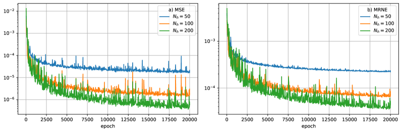
Figure 1: Learning curves for the Lorenz network model corresponding to ODEs (27). The curves are computed at validation steps, i.e., for inputs that did not used for updating the network parameters. Panel (a) represents MSE, Eq. (17). Panel (b) shows MRNE, Eq. (19). Different curves correspond to different $N_{h}$.

The training result is shown in Figs. 2 and 3. Figure 2(a, b) demonstrates the Lorenz attractor computed for the standard set of parameters $\sigma=10$, $r=28$, $b=8/3$ using fourth order Runge-Kutta method (a) and the network model (22) (b). Observe very high coincidence of two plots.

Neural networks architecture is very good suited for parallel computations. So doing computations with the network model we employ it considering multiple trajectories at once: to plot Fig. 2(a) via the Runge-Kutta method we compute $10000$ steps with the time interval $\Delta t=0.01$, while in Fig. 2(b) we compute $100$ trajectories at once, each of the length $100$ steps $\Delta t=0.01$.

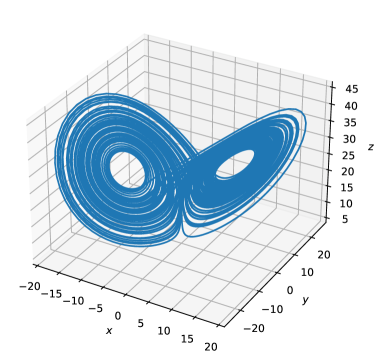
a) b)

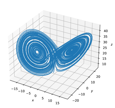
Figure 2: Lorenz attractor computed (a) as a numerical solution of Eqs. (27) using the forth order Runge-Kutta method and (b) as iteration of the network model (22). Parameters are $\sigma=10$, $r=28$, $b=8/3$.

Figure 3 shows Fourier spectra computed for $x$ at the parameters $\sigma=10$, $r=28$, $b=8/3$, panels (a, b), and $\sigma=16$, $r=45.92$, $b=4$, panels (c, d). Left panels (a) and (c) are computed for the Runge-Kutta data and the right ones are obtained for the network model. The spectra coincide very well that indicates that the obtained network (22) models the Lorenz dynamics very well.

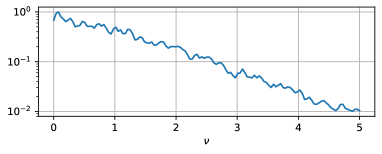
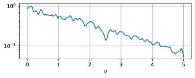
a) b)
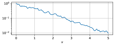
c) d)

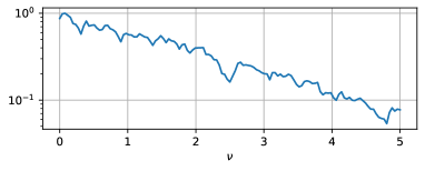
Figure 3: Fourier spectra of the Lorenz attractor. Data series for panels (a) and (c) are computed numerically using the forth order Runge-Kutta method, and data for the panels (b) and (d) are obtained after iterations of the network model (22). Parameter for the panels (a) and (b) are $\sigma=10$, $r=28$, $b=8/3$, and panels (c) and (d) are obtained with $\sigma=16$, $r=45.92$, $b=4$

Now compute Lyapunov exponents using the standard algorithm[19, 20]. Using the Runge-Kutta method and at $\sigma=10$, $r=28$, $b=8/3$ we obtain the values of $\lambda_{i}$ in Eq. (29). Lyapunov exponents $\tilde{\lambda}_{i}$ computed for the network model (22) and corresponding variational equation (26) are in Eq. (30). Observe the very good coincidence. Notice that $\lambda_{2}$ is expected to be zero since describes marginally stable perturbations along trajectories. However actual values in computations are never exact zero. Their closeness to zero indicates the quality of the computation. In our case both $\lambda_{2}$ and $\tilde{\lambda}_{2}$ are very small.

$$\lambda_{1} =0.906 \lambda_{2} =8.26\times 10^{-6} \lambda_{3} =-14.6$$ (29)

$$\tilde{\lambda}_{1} =0.905 \tilde{\lambda}_{2} =1.26\times 10^{-5} \tilde{\lambda}_{3} =-14.6$$ (30)

Similarly the Lyapunov exponents are computed for the parameters $\sigma=16$, $r=45.92$, $b=4$. Observe again the very high similarity of $\lambda_{i}$ with network model exponents $\tilde{\lambda}_{2}$:

$$\lambda_{1} =1.50 \lambda_{2} =-1.89\times 10^{-5} \lambda_{3} =-22.5$$ (31)

$$\tilde{\lambda}_{1} =1.49 \tilde{\lambda}_{2} =4.34\times 10^{-5} \tilde{\lambda}_{3} =-22.7$$ (32)

4.2 Röessler system

Another system that we consider is the Röessler system [25, 24, 26]:

$$\begin{gathered}\dot{x}=-y-z,\\ \dot{y}=x+ay,\\ \dot{z}=b+z(x-c),\end{gathered}$$ (33)

For this system we choose the following $\mu_{u,p}$ and $s_{u,p}$ and compute the corresponding $\mu_{g}$ and $s_{g}$:

$$\begin{gathered}\mu_{u}=(0,0,0),\;s_{u}=(10,10,10),\\ \mu_{p}=(0,0,0),\;s_{p}=(10,10,10),\\ \mu_{g}=(0,0,0),\;s_{g}=(14,101,142).\end{gathered}$$ (34)

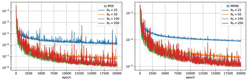
Figure 4: Learning curves for the Röessler network model corresponding to ODEs (33).

Figure 4 demonstrates the learning curves for the Röessler system. We observe that the training now goes much faster then for the Lorenz system, see Fig. 1. Inspecting the learning curves we can conclude that the network models with $N_{h}=100$ and $200$ do not differ much. So, unlike the Lorenz system we will consider the network model for the Röessler system with $N_{h}=100$. After 20000 epochs of the training we save the model with the smallest MRNE equals to approximately $1.0\times 10^{-5}$.

Figure 5 demonstrates chaotic Röessler attractor and the corresponding Fourier spectra computed for ODEs (33) (left column) and for the trained network model (right column). Numerical solutions of ODEs here and below are obtained using the forth order Runge-Kutta method. A very high similarity of the graphs indicates the high quality of approximation of the network model. Another example of dynamics is in Fig. 6. Parameters here correspond to the period 2 oscillations. Limit cycles in Figs. 6(a) and (c) looks almost identical. The spectrum for the network model in Figs. 6(d) also repeats the spectrum in Fig. 6(b) in location and relative heights of harmonics. The difference between these two spectra is in small fluctuations. Since the regime of the considered system is periodic the fluctuations are mere artifacts related in particular with the computation method. The methods of computations are different and so the fluctuations are.

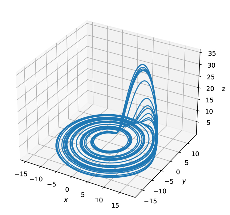
a) b)

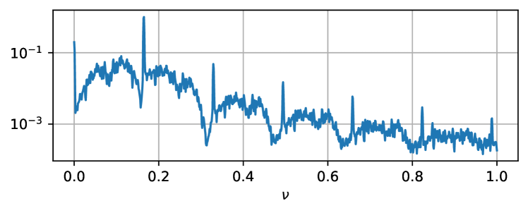
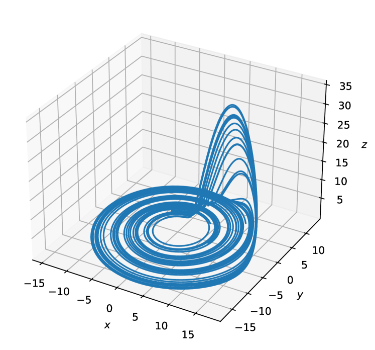
c) d)

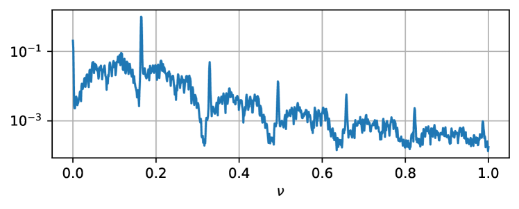
Figure 5: Röessler chaotic attractor at $a=0.15$, $b=0.2$, and $c=10$, panels (a) and (c) and the corresponding Fourier spectra, panels (b) and (d). Panels (a) and (b): numerical solution of ODEs (33). Panels (c) and (d): iterations of a trained network model.

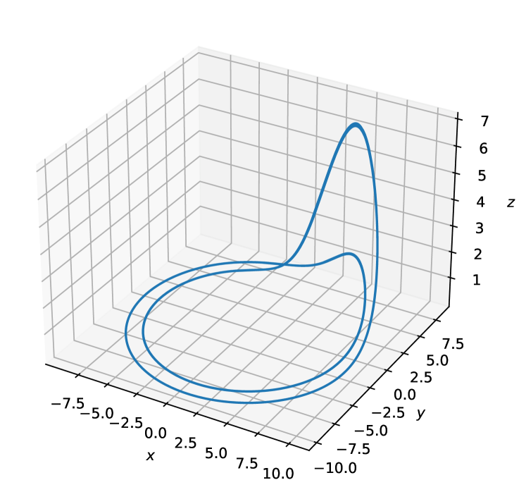
a) b)

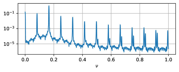
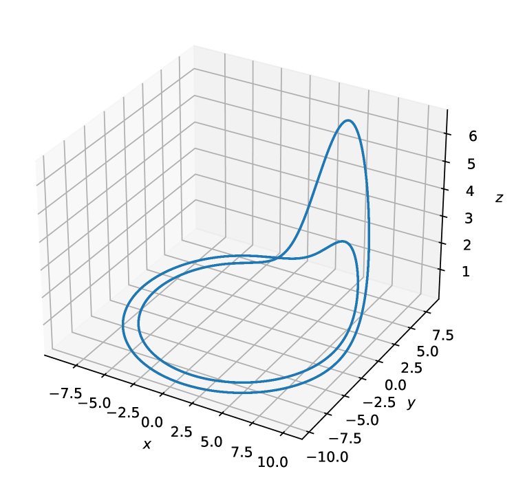
c) d)

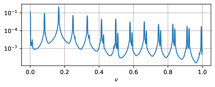
Figure 6: Period 2 oscillations of the Röessler system at $a=0.1$, $b=0.1$, and $c=6$. Limit cycle (a) and Fourier spectrum (b) are computed for ODEs and the corresponding panels (c) and (d) are obtained for the network model.

To demonstrate that the trained network model reproduces the dynamics of the modeled ODEs in a wide range of parameter in Fig. 7 we show a bifurcation diagram for the Röessler system. Parameters $a$ and $b$ are fixed and $c$ is varying. For each $c$ we compute a trajectory then find its Poincaré section at $x=0$. Absent values of variables between the time discretization points are obtained via linear interpolation. The diagram obtained for the numerical solution of (33), see Fig. 7(a) is reproduced very well by the network model, see Fig. 7(b). Notice however that the bifurcation points for the network model are little bit shifted to the right. Nevertheless the overall correspondence is very high.

a)
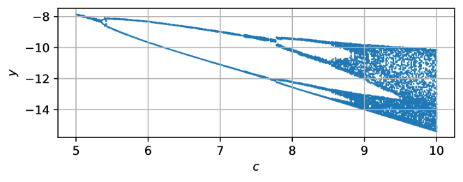
b)

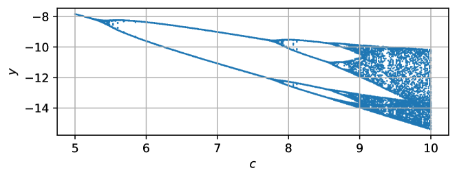
Figure 7: Bifurcation diagrams for the Röessler system at $a=0.1$ and $b=0.1$. Panel (a) corresponds to a numerical solution of ODEs (33) and panel (b) is computed for the network model. Bifurcation diagrams are obtained as $y$ values at Poincaré sections at $x=0$. The sections are computed for linearly interpolated time series.

Let us now compare Lyapunov exponents applying the standard algorithm for ODEs (33) and for the corresponding network model. We demonstrate two cases. For parameters $a=0.15$, $b=0.2$, $c=10$ the Lyapunov exponents $\lambda_{i}$ for ODEs are shown in Eq. (35). For comparison the exponents $\tilde{\lambda}_{i}$ for the corresponding network model at the same parameters are shown in Eq. (36). The values coincide very well. Because the considered system is autonomous the value of $\lambda_{2}$ must be zero. Actually computed values are indeed very close to zero.

$$\lambda_{1} =0.0886 \lambda_{2} =-8.66\times 10^{-7} \lambda_{3} =-9.80$$ (35)

$$\tilde{\lambda}_{1} =0.0839 \tilde{\lambda}_{2} =2.70\times 10^{-5} \tilde{\lambda}_{3} =-9.64$$ (36)

One more example is considered at $a=0.1$, $b=0.1$, $c=13$ for that the Röessler systems also has a chaotic attractor. From Eqs. (37) and (38) we again observe that the exponents for the network model $\tilde{\lambda}_{i}$ are close to those obtained for the numerical solution of ODEs $\lambda_{i}$.

$$\lambda_{1} =0.0116 \lambda_{2} =1.87\times 10^{-5} \lambda_{3} =-12.8$$ (37)

$$\tilde{\lambda}_{1} =0.0189 \tilde{\lambda}_{2} =8.53\times 10^{-5} \tilde{\lambda}_{3} =-12.8$$ (38)

However we must notice that the correspondence of the Lyapunov exponents for the Röessler system is not so good as for the Lorenz system, see. Eqs. (29)- (32). We address it to the parameter mismatch observed in the bifurcation diagrams.

4.3 Hindmarch–Rose neuron

Now we consider the Hindmarsh–Rose model of neuronal activity [27, 28]:

$$\begin{gathered}\dot{x}=y-ax^{3}+bx^{2}-z+I,\\ \dot{y}=c-dx^{2}-y,\\ \dot{z}=r(s(x-\alpha)-z)\end{gathered}$$ (39)

Totally this system has eight parameters. However often the system is considered when six of them have standard values: $a=1.0$, $b=3.0$, $c=1.0$, $d=5.0$, $s=4.0$, $\alpha=-1.6$. Parameters $I$ and $r$ are varied.

The Hindmarch–Rose model (39) is a simplified model for biological neurons presenting bursting oscillations. In this regime, bursts of fast spikes are followed by quiescent periods. Typical values of parameters where the bursts are observed are $I=2.7$ and $r=0.003$. Thus we select the normalization to be close to these values:

$$\begin{gathered}\mu_{u}=(0,-5,2.5),\;s_{u}=(0.8,2.5,0.5),\\ \mu_{p}=(0.012,2.7),\;s_{p}=(0.024,0.3),\\ \mu_{g}=(-2.9,2.8,0.047),\;s_{g}=(4.2,5.2,0.13)\end{gathered}$$ (40)

Learning curves for the network model of the system (39) are shown in Fig. 8. Unlike two previous cases the training occurs much faster: it takes 7000 epochs for the loss function at $N_{h}=100$ to reach values about $10^{-10}$. The model at $N_{h}=50$ also demonstrates a very good convergence, and the model at $N_{h}$ behave much worse. Thus we will consider a model with $N_{h}=50$.

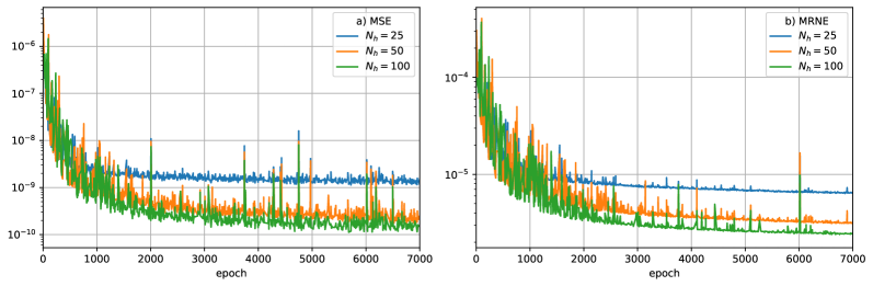
Figure 8: Learning curves for the Hindmarch-Rose network model corresponding to ODEs (39).

Figure 9(a, b) demonstrates typical solutions of the Hindmarch-Rose model (39): Panel (a) demonstrates periodical the bursts of spikes and in the panel (b) we see chaotic spikes. The system contains fast and slow variables, i.e., is stiff. To solve it numerically the method LSODA is used [29].

Figures 9(c, d) shows the corresponding time series obtained from the neural network model. The behavior of the network model is very similar, but the close inspection revels that in the panel (c) there are seven spikes in each burst, while the “original” curve contains only six of them. It means that although the model demonstrates a neural dynamics as well as in original ODEs, its parameters do not coincide exactly. The chaotic regimes in the panels (b) and (d) obviously represent the same regime.

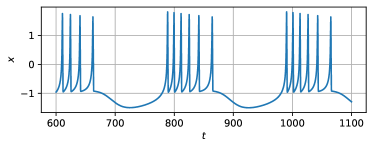
a) b)

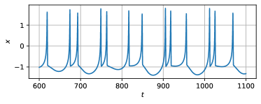
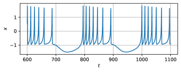
c) d)

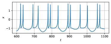
Figure 9: Time series of $x(t)$ obtained as numerical solution of ODEs (39), panels (a) and (b), and corresponding iterations of the neural network model, panels (c) and (d). Parameters are $r=0.003$, $I=2.7$ for panels (a) and (d), and $r=0.013$, $I=2.9$ in panels (b) and (d).

In Fig. 10(a) and (b) bifurcation diagrams provides a more detailed comparison of the neural network model with ODEs. In both panels the diagrams are computed for Poincaré sections at $x=0$ computed for linearly interpolated times series. The diagrams have similar global structure. One can see areas of bursts in their left parts and chaotic areas to the right. However the detailed arrangement is different. The diagram for the neural network model looks less regular along parameter axis. Often changes of the regimes are observed.

a)
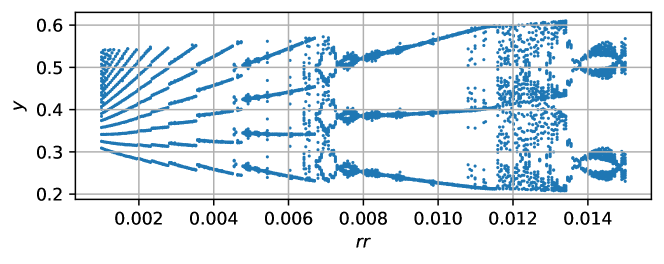
b)

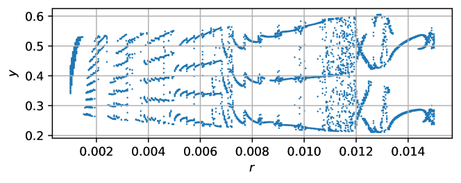
Figure 10: Bifurcation diagrams for the Röessler system at $a=0.1$ and $b=0.1$. Panel (a) corresponds to a numerical solution of ODEs (33) and panel (b) is computed for the network model. Bifurcation diagrams are obtained as $y$ values at Poincaré sections at $x=0$. The sections are computed for linearly interpolated time series.

Finally we compare Lyapunov exponents computed for numerical solutions of ODEs (39) and for iterations of the neural network model. For chaotic spikes at $r=0.013$, $I=2.9$, see Fig. 9(b), the Lyapunov exponents $\lambda_{i}$ are given by Eq. (41). The corresponding exponents for the network model $\tilde{\lambda}_{i}$ are gathered in Eq. (42). The exponents are pairwise close but do not coincide.

$$\lambda_{1} =8.39\times 10^{-3} \lambda_{2} =-1.32\times 10^{-5} \lambda_{3} =-9.55$$ (41)

$$\tilde{\lambda}_{1} =7.95\times 10^{-3} \tilde{\lambda}_{2} =9.77\times 10^{-6} \tilde{\lambda}_{3} =-9.63$$ (42)

Similar situations is obtained for another parameter values $r=0.012$, $I=2.7$: the exponents $\lambda_{i}$ and $\tilde{\lambda}_{i}$ are similar, but the difference is notable.

$$\lambda_{1} =5.41\times 10^{-3} \lambda_{2} =7.59\times 10^{-6} \lambda_{3} =-10.2$$ (43)

$$\tilde{\lambda}_{1} =3.20\times 10^{-3} \tilde{\lambda}_{2} =3.04\times 10^{-5} \tilde{\lambda}_{3} =-10.3$$ (44)

We address this not very good coincides of the Lyapunov exponents to the very weak chaos. The first exponents are very small by magnitude so that the numerical routine converges poorly and is strongly affected by numerical errors. The parameter mismatch observed above for the Röessler system also includes in the not very good coincides of the Lyapunov exponents.

Thus, we observe that the discussed neural network model for the Hindmarch-Rose system provides good qualitative approximation of this system, however the quantitative correspondence is not high.

5 Conclusion

We discussed the universal neural network, a perceptron with one hidden level, that can be trained to model behavior of various dynamical systems given by ODEs. Mathematically the universal neural network model is a discrete time system, see (22). We aware of contemporary success in using of so called deep networks. Our network on contrary is not deep. We have preferred it because there is a rigorous mathematical evidence, the Universal Approximation Theorem, that the network with such architecture is able to approximate various dependencies. Another reason to apply a classical perceptron is its simple structure. We believe that it will help to trigger new theoretical studies of dynamical systems. From the practical point of view this simple network can be effectively simulated using so called AI accelerators, a hardware dedicated to deal with artificial neural networks. The approach developed in this paper can be considered as an alternative numerical method of modeling dynamical system that is able to utilize contemporary parallel hard- and software.

The universal network model was trained to reproduce the dynamics of the three systems: Lorenz and the Röessler systems and Hindmarch-Rose model. It was very successful for the Lorenz system. This is confirmed by visual inspection of attractors, and by coincidence of Fourier spectra and Lyapunov exponents. For the Röessler system the correspondence is also high. However a certain mismatch of the bifurcation points is observed on bifurcation diagrams computed for the numerical solution of Röessler ODEs and for the network model.

For the Hindmarch-Rose system good qualitative correspondence is achieved however quantitative characteristics are sometimes differ. This system allows to reveal the limitations of the suggested approach. Hindmarch-Rose system is stiff and also its regimes changes fast withing a narrow range parameters. Probably for such cases like this system a more subtle approach is required.

Work of PVK on theoretical formulation and numerical computations and work of NVS on results analysis was supported by grant of Russian Science Foundation No 20-71-10048.

References

- [1] Simon Haykin. Neural networks and learning machines. Pearson Prentice Hall, third edition, 2009.
- [2] G. Peter Zhang. Neural networks for time-deries forecasting, pages 461–477. Springer Berlin Heidelberg, Berlin, Heidelberg, 2012.
- [3] Nigel Da Costa Lewis. Deep time series forecasting with Python: An intuitive introduction to deep learning for applied time series modeling. ND Lewis, 2016.
- [4] Jason Brownlee. Deep learning for time series forecasting: predict the future with MLPs, CNNs and LSTMs in Python. Machine Learning Mastery, 2018.
- [5] Martín Abadi, Ashish Agarwal, Paul Barham, Eugene Brevdo, Zhifeng Chen, Craig Citro, Greg S. Corrado, Andy Davis, Jeffrey Dean, Matthieu Devin, Sanjay Ghemawat, Ian Goodfellow, Andrew Harp, Geoffrey Irving, Michael Isard, Yangqing Jia, Rafal Jozefowicz, Lukasz Kaiser, Manjunath Kudlur, Josh Levenberg, Dandelion Mané, Rajat Monga, Sherry Moore, Derek Murray, Chris Olah, Mike Schuster, Jonathon Shlens, Benoit Steiner, Ilya Sutskever, Kunal Talwar, Paul Tucker, Vincent Vanhoucke, Vijay Vasudevan, Fernanda Viégas, Oriol Vinyals, Pete Warden, Martin Wattenberg, Martin Wicke, Yuan Yu, and Xiaoqiang Zheng. TensorFlow: Large-scale machine learning on heterogeneous systems, 2015. Software available from tensorflow.org.
- [6] Adam Paszke, Sam Gross, Soumith Chintala, Gregory Chanan, Edward Yang, Zachary DeVito, Zeming Lin, Alban Desmaison, Luca Antiga, and Adam Lerer. Automatic differentiation in PyTorch. In NIPS-W, 2017.
- [7] Y. Wei, J. Zhou, Y. Wang, Y. Liu, Q. Liu, J. Luo, C. Wang, F. Ren, and L. Huang. A review of algorithm & hardware design for AI-based biomedical applications. IEEE Transactions on Biomedical Circuits and Systems, 14(2):145–163, 2020.
- [8] Manar Abu Talib, Sohaib Majzoub, Qassim Nasir, and Dina Jamal. A systematic literature review on hardware implementation of artificial intelligence algorithms. The Journal of Supercomputing, 77:1897–1938, 2021.
- [9] Morris Kline. Mathematical thought from ancient to modern times: Volume 2, volume 2. Oxford university press, 1990.
- [10] A. N. Kolmogorov. On the representation of continuous functions of several variables by superpositions of continuous functions of a smaller number of variables. Doklady Akademii Nauk SSSR, 108:179–182, 1956. English translation: Amer. Math. Soc. Transl., 17 (1961), pp. 369-373.
- [11] A. N. Kolmogorov. On the representation of continuous functions of many variables by superposition of continuous functions of one variable and addition. Doklady Akademii Nauk SSSR, 114:953–956, 1957. English translation: Amer. Math. Soc. Transl., 28 (1963), pp. 55–59.
- [12] V. I. Arnold. On functions of three variables. Doklady Akademii Nauk SSSR, 114:679–681, 1957. English translation: Amer. Math. Soc. Transl., 28 (1963), pp. 51–54.
- [13] R. Hecht-Nielson. Kolmogorov’s mapping neural network eistence theorem. In First IEEE international conference on neural networks, volume III, pages 11–14. San Diego, CA, 1987.
- [14] G. Cybenko. Approximation by superpositions of a sigmoidal function. Mathematics of Control, Signals and Systems, 2(4):303–314, December 1989.
- [15] K. Funahashi. On the approximate realization of continues mappings by neural networks. Neural Networks, 2:183–192, 1989.
- [16] Kurt Hornik, Maxwell Stinchcombe, and Halbert White. Multilayer feedforward networks are universal approximators. Neural Networks, 2(5):359–366, 1989.
- [17] W. Light. Ridge functions, sigmoidal functions and neural networks, volume VII of Approximation Theory, pages 163–206. Academic Press, Boston, 1992.
- [18] Diederik P. Kingma and Jimmy Ba. Adam: A method for stochastic optimization. arXiv preprint arXiv:1412.6980, 2014. Published as a conference paper at International Conference on Learning Representations (ICLR) 2015.
- [19] Giancarlo Benettin, Luigi Galgani, Antonio Giorgilli, and Jean-Marie Strelcyn. Lyapunov characteristic exponents for smooth dynamical systems and for Hamiltonian systems: a method for computing all of them. Part 1: Theory. Meccanica, 15(1):9–20, 1980.
- [20] Ippei Shimada and Tomomasa Nagashima. A numerical approach to ergodic problem of dissipative dynamical systems. Prog. Theor. Phys., 61(6):1605–1616, 1979.
- [21] John Nickolls, Ian Buck, Michael Garland, and Kevin Skadron. Scalable parallel programming with CUDA. ACM Queue, 6(2):40–53, 2008.
- [22] E. N. Lorenz. Deterministic nonperiodic flow. Journal of the atmospheric sciences, 20(2):130–141, 1963.
- [23] C. Sparrow. The Lorenz equations: bifurcations, chaos, and strange attractors. Springer-Verlag, NY, Heidelberg, Berlin, 1982.
- [24] H. G. Schuster and W. Just. Deterministic chaos: an introduction. Wiley-VCH, 2005.
- [25] O. E. Rössler. An equation for continuous chaos. Physics Letters A, 57(5):397–398, 1976.
- [26] S. P. Kuznetsov. Dynamical chaos. Moscow: Fizmatlit, 2006.
- [27] J. L. Hindmarsh and R. M. Rose. A model of neuronal bursting using three coupled first order differential equations. Proc. R. Soc. Lond. B, 221:87–102, 1984.
- [28] X.-J. Wang. Genesis of bursting oscillations in the Hindmarsh-Rose model and homoclinicity to a chaotic saddle. Physica D: Nonlinear Phenomena, 62(1):263–274, 1993.
- [29] L. Petzold. Automatic selection of methods for solving stiff and nonstiff systems of ordinary differential equations. SIAM Journal on Scientific and Statistical Computing, 4(1):136–148, 1983.