Slow periodic oscillation without radiation damping: New evolution laws for rate and state friction–B

Slow periodic oscillation without radiation damping: New evolution laws for rate and state friction

The dynamics of sliding friction is mainly governed by the frictional force. Previous studies have shown that the laboratory-scale friction is well described by an empirical law stated in terms of the slip velocity and the state variable. The state variable represents the detailed physicochemical state of the sliding interface. Despite some theoretical attempts to derive this friction law, there has been no unique equation for time evolution of the state variable. Major equations known to date have their own merits and drawbacks. To shed light on this problem from a new aspect, here we investigate the feasibility of periodic motion without the help of radiation damping. Assuming a patch on which the slip velocity is perturbed from the rest of the sliding interface, we prove analytically that three major evolution laws fail to reproduce stable periodic motion without radiation damping. Furthermore, we propose two new evolution equations that can produce stable periodic motion without radiation damping. These two equations are scrutinized from the viewpoint of experimental validity and the relevance to slow earthquakes.

1 Introduction

1.1 Evolution equations for rate- and state-dependent friction law

Since slip behaviours of earthquake faults are mainly dominated by the frictional force, study of friction laws plays a vital role in understanding earthquakes from physical point of view. Data from laboratory experiments on quasi-static slip and isothermal condition of rocks are well summarized into an empirical law, which is referred to as the rate- and state-dependent friction law (hereafter the RSF law) (Dieterich, 1979).

$$\mu=\mu_{0}+a\log(\frac{\hat{V}}{V_{0}})+b\log(\frac{V_{0}\hat{\theta}}{L}),$$ (1)

where $\hat{V}$ is the slip velocity, $\hat{\theta}$ is the state variable, $L$ is the characteristic length, and $V_{0}$ and $\mu_{0}$ are constants involving an arbitrary reference state. Two nondimensional parameters $a$ and $b$ depend on materials and various experimental condition. The logarithmic nature of this law reflects a thermal activation process at asperities (Heslot et al., 1994). In view of mathematical convenience, we adopt the natural logarithm unless otherwise indicated.

The state variable $\theta$ has the dimension of time representing the condition of the slipping surface. The behaviour of the state variable is described by a time evolution equation.

$$\derivative{\hat{\theta}}{\hat{t}}=f(\mathbf{X}(t)),$$ (2)

where $\mathbf{X}(t)$ denotes relevant macroscopic variables such as the slip velocity, state variable(s), or the shear stress. We then need to choose an appropriate function for the right hand side. However, since there is no rigorous definition of the state variable, derivation of a time evolution equation cannot be systematic but only heuristic. As a result, there has been no decisive form for the function $f$ in Eq. (2).

Here we briefly review some of the most commonly used equations (Ruina, 1983):

$$\derivative{\hat{\theta}}{\hat{t}} = -\frac{\hat{V}\hat{\theta}}{L}\log(\frac{\hat{V}\hat{\theta}}{L}),$$ (3)

$$\derivative{\hat{\theta}}{\hat{t}} = 1-\frac{\hat{V}\hat{\theta}}{L}.$$ (4)

The former equation, referred to as the slip law, leads to an exponential relaxation of the friction force after an abrupt velocity change. The latter equation is referred to as the aging law. It describes monotonic increase of the state variable, which is interpreted as time-dependent healing or aging. The slip law does not describe such a healing effect. These laws have their own merits and drawbacks, but somewhat describe experimental results under isothermal and low-velocity conditions.

Less common but more recent equation is the following (Nagata et al., 2012).

$$\derivative{\hat{\theta}}{\hat{t}}=1-\frac{\hat{V}\hat{\theta}}{L}-\frac{\gamma}{b\sigma}\derivative{\hat{\tau}}{\hat{t}}\hat{\theta},$$ (5)

where $\gamma$ is a positive constant, $\sigma$ is the normal stress, and $\tau$ is the shear stress.

These three evolution laws have their own merits and drawbacks (Marone, 1998; Bizzarri, 2011). At a steady state, however, each equation gives $\hat{\theta}=L/\hat{V}$, leading to

$$\mu=\mu_{0}+(b-a)\log(\frac{\hat{V}}{V_{0}}).$$ (6)

1.2 Feasibility of periodic motion with RSF law

Using the RSF law as a boundary condition, the motion of faults is defined and solved numerically based on the elasticity theory (Cochard & Madariaga, 1994). Linear stability analysis under some simple configurations (e.g., anti-plane shear) reveals that uniform and steady slip can be unstable via a Hopf bifurcation, where long-wavelength perturbations grow exponentially with time (Rice & Ruina, 1983; Rice et al., 2001).

To characterize the oscillatory motion due to Hopf bifurcation, linear stability analysis alone is not sufficient since the oscillation is mainly governed by nonlinear effects in the friction force. To this end, nonlinear analysis must be implemented (Gu et al., 1984; Ranjith & Rice, 1999; Viesca, 2016a, b). In particular, for a single degree of freedom system, Gu et al. (1984) and Ranjith & Rice (1999) construct quantities similar to a Lyapunov function and show rigorously that any trajectory moves away from the unstable fixed point. Their results also imply that the limit cycle is absent and the trajectory diverges. This is rather a major drawback of existing time evolution equations for the RSF. This has been already pointed out by Rice (1993), but does not appear to be commonly recognized.

To prevent the divergence of trajectory and to yield the stable cycle of oscillation, some extra ingredients have been introduced. For instance, if inertia is introduced to the equation, it yields a steady oscillatory motion. However, the equation with inertia corresponds to the motion of a rigid body pulled with an elastic spring (Sugiura et al., 2014), but cannot be a model for a slip patch. More commonly used technique is to introduce a viscous resistance that is proportional to the slip velocity. This resistance is called as the ”radiation damping” (Rice, 1993), which can be derived from the dynamic elasticity theory (Cochard & Madariaga, 1994). A popular model for slow earthquakes, which is referred to as a quasi-static (or quasi-dynamic) model, assumes the static Green’s function together with the radiation damping. It may be, however, an ad hoc hybrid of dynamic/static elasticity. More importantly, use of radiation damping in modelling slow aseismic events may be somewhat contradictory since they do not radiate seismic waves.

Some studies have shown that, if the friction is velocity strengthening at higher velocities, aseismic slow oscillation can be realized (Matsuzawa et al., 2010; Shibazaki & Shimamoto, 2007; Barbot, 2019a). However, these models also adopt radiation damping. To the best of our knowledge, there have been very few studies that reproduce aseismic slip cycles without radiation damping (Hawthorne & Rubin, 2013). However, the model settings in Hawthorne & Rubin (2013) appear rather special in terms of the spatial distribution of frictional parameters and the boundary conditions. It is thus not clear how general such a model can reproduce an aseismic slip cycle without radiation damping. Some models may be able to reproduce transitory cycles of aseismic slips, but such a transitory cycle is not our aim here. Rather, we wish to reproduce a steady aseismic cycle in the sense that it is repeatable for arbitrary times.

In this paper, we shed new light on this problem. Using a mathematical theorem, we show analytically that the limit cycle does not exist in a single degree of freedom system with popular evolution equations. We then propose new evolution equations and show that they reproduce periodic motion repeatedly within the time of simulation (more than one hundred times). We also show that, in contrast to some previous studies, velocity-strengthening is not an essential ingredient to realize a slow aseismic slip. In Section 2, we formulate the problem by introducing the fault patch model and review some previous results. In Section 3, we prove that three major evolution laws cannot yield any periodic motion. In Section 4, we propose two new evolution laws that can realize periodic motion. We then discuss the behaviours of these new equations in the context of velocity step experiments and examine the validity of these laws. In Section 5, we discuss the relevance of these new equations in the context of slow earthquakes (Obara & Kato, 2016).

2 Model

2.1 Single degree of freedom system

Since nonlinear analysis of partial differential equations is not straightforward, slip dynamics on a spatially extended system is often reduced to a single degree of freedom system (Scholz, 1990). This is done by considering that the slip velocity on a fault plane is perturbed only in a finite circular area, and the rest of the fault plane is displaced at a constant slip velocity, $V_{p}$. The relevant variables are then the perturbed slip velocity $\dot{\hat{u}}$ and the displacement ${\hat{u}}$ at the patch center.

The shear stress $\tau$ on the patch is proportional to the perturbed displacement with the effective stiffness $\hat{k}$: $\tau=\hat{k}(V_{p}\hat{t}-\hat{u})$. Since the applied shear stress and frictional force must balance on the fault plane, the following equation holds:

$$\frac{\hat{k}}{\sigma}(V_{p}\hat{t}-\hat{u})=\mu_{0}+a\log(\frac{\hat{V}}{V_{0}})+b\log(\frac{V_{0}\hat{\theta}}{L}),$$ (7)

where $\hat{V}=d\hat{u}/dt$ and $\sigma$ is the normal stress.

2.2 Definition of dimensionless variables

Hereafter we use dimensionless variables given as follows

$$u=\frac{\hat{u}}{L},\,V=\frac{\hat{V}}{V_{p}},\,\theta=\frac{\hat{\theta}V_{p}}{L},\,k=\frac{\hat{k}L}{\sigma},\,t=\frac{\hat{t}V_{p}}{L}.$$ (8)

Here, $V_{p}$, $k$, and $L$ are the steady-state slip velocity, the spring constant, and the characteristic length, respectively.

2.3 Governing equations

Assuming that the velocity and the state variable change smoothly, we may differentiate the equation with respect to time. Using (8), we can derive the nondimensional equations.

$$\derivative{V}{t}=\frac{k}{a}(1-V)V-\frac{b}{a\theta}f(V,\theta)V,$$ (9)

$$\derivative{\theta}{t}=f(V,\theta).$$ (10)

After differentiation, the system is reduced to an autonomous system with two variables, making the analysis easier.

A linear stability analysis of this system reveals that a Hopf bifurcation occurs when the stiffness $k$ is smaller than the critical value $k_{c}$ (Ruina, 1983). However, in normal linear stability analysis, one can know the flow field only in a closed proximity of the fixed point. To know the solution realized in the linearly unstable regime, one needs to know the global flow field.

3 Absence of periodic motion: proof

Here we scrutinize three major evolution equations as to whether they can yield stable periodic solutions.

3.1 Dulac’s criterion and its implication

In two dimensional dynamical systems, some useful theorems guarantee the absence of closed orbits. Here we make use of the following Dulac’s criterion (Strogatz, 2001). The proof is described in Supplemental Information.

Theorem 3.1

Dulac’s criterion
The vector $\mathbf{x}$ is defined in a set $A$, which is a simply connected area on $R^{2}$. Time evolution of the vector $\mathbf{x}$ is described by $\mathbf{\dot{x}}=\mathbf{f}(\mathbf{x})$, where $\mathbf{f}(\cdot)$ is a differentiable vector field. Let $g(\mathbf{x})$ be a real-valued function. If the sign of $\nabla\dotproduct({g\mathbf{\dot{x}}})$, either positive or negative, is the same at any point on $A$, then there is no closed orbit.

If there is no closed orbit, a limit cycle cannot exit. We can thus prove the absence of limit cycle by making use of the above theorem. In the present context, the vector field $\mathbf{\dot{x}}$ is given by Eqs. (9) and (10). Then, to prove the absence of the limit cycle, we need to find a function $g(\cdot)$ that satisfies the criterion.

Since the present system is described by two variables, the trajectory is limited to the two-dimensional space, $(V,\theta)$. According to the theory of dynamical systems (Strogatz, 2001), the asymptotic behavior of two-dimensional systems is limited to three cases: fixed point, limit cycle, and divergence to infinity. (Note that strange attractor is ruled out in two dimensional space). Therefore, if the fixed point becomes unstable and the limit cycle does not exist, the trajectory must diverge after a sufficiently long time. This holds for all the three cases below.

Note that, since $V>0$, it is sufficient to consider the first quadrant in $(V,\theta)$ space; i.e., $V>0$ and $\theta>0$.

3.2 Case 1: Slip law

In the case of slip law, the governing equations are

$$\derivative{V}{t}=\frac{k}{a}(1-V)V+\frac{bV^{2}}{a}\log(V\theta),$$ (11)

$$\derivative{\theta}{t}=-V\theta\log(V\theta).$$ (12)

This system has a unique fixed point at $(V,\theta)=(1,1)$. Jacobi matrix J is then derived as

$$J\equiv\left(\begin{array}[]{cc}\displaystyle\partialderivative{\dot{V}}{V}&\displaystyle\partialderivative{\dot{V}}{\theta}\\ \displaystyle\partialderivative{\dot{\theta}}{V}&\displaystyle\partialderivative{\dot{\theta}}{\theta}\\ \end{array}\right)_{(V,\theta)=(1,1)}=\left(\begin{array}[]{cc}\displaystyle{\frac{b-k}{a}}&\displaystyle{\frac{b}{a}}\\ -1&-1\\ \end{array}\right).$$ (13)

Therefore the eigenvalues are

$$\lambda=\frac{1}{2}\left[\frac{b-a-k}{a}\pm\sqrt{\left(\frac{b-a-k}{a}\right)^{2}-4\frac{k}{a}}\right].$$ (14)

Thus, if the spring constant $k$ is smaller than the critical value $k_{c}=b-a$, $\Re{\lambda}$ and $\Re{\bar{\lambda}}$ are positive and the fixed point is unstable. In other words, Hopf bifurcation occurs at $k=k_{c}$, below which steady slip is unstable.

We then prove the absence of limit cycle in this system based on the Dulac’s criterion. By choosing

$$g(V,\theta)=\frac{a}{V}\theta^{(b/a-1)},$$ (15)

the divergence of $g\mathbf{\dot{x}}$ is calculated as

$$\nabla\dotproduct({g\mathbf{\dot{x}}})=\theta^{(\frac{b}{a}-1)}(b-a-k)=\theta^{(\frac{b}{a}-1)}\epsilon,$$ (16)

where $\epsilon$ is a constant defined as $\epsilon=k_{c}-k$. The divergence Eq. (16) is always positive except at the bifurcation point, $k=k_{c}$. Namely, there is no limit cycle if $k<k_{c}$.

3.3 Case 2: Aging law

In the case of aging law, the governing equations are

$$\derivative{V}{t}=\frac{k}{a}(1-V)V-\frac{b}{a\theta}(1-V\theta)V,$$ (17)

$$\derivative{\theta}{t}=1-V\theta.$$ (18)

This system also has a unique fixed point at $(V,\theta)=(1,1)$. Jacobi matrix J is then derived as

$$J=\left(\begin{array}[]{cc}\displaystyle{\frac{b-k}{a}}&\displaystyle{\frac{b}{a}}\\ -1&-1\\ \end{array}\right)$$ (19)

Then we calculate the eigenvalues of J and find the Hopf bifurcation point as $k_{c}=b-a$.

We can again prove the absence of limit cycle in this model by setting

$$g(V,\theta)=\frac{a}{V}.$$ (20)

This leads to

$$\nabla\dotproduct({g\mathbf{\dot{x}}})=-k+b-a=\epsilon,$$ (21)

where $\epsilon$ is constant defined as $\epsilon=k_{c}-k$. The divergence Eq. (21) is always positive for $k<k_{c}$. This result means that there is no limit cycle once the fixed point is unstable.

3.4 Case 3: Nagata’s law

In the case of Nagata’s law, the governing equations are

$$\derivative{V}{t}=\frac{k}{a}(1-V)V-\frac{b}{a\theta}\left[1-V\theta-\frac{\gamma k}{b}(1-V)\theta\right]V,$$ (22)

$$\derivative{\theta}{t}=1-V\theta-\frac{\gamma k}{b}(1-V)\theta.$$ (23)

This system has a unique fixed point at $(V,\theta)=(1,1)$. At this point the Jacobi matrix is

$$J=\left(\begin{array}[]{cc}\displaystyle{\frac{-k+b-\gamma k}{a}}&\displaystyle{\frac{b}{a}}\\ \displaystyle-1+\frac{\gamma k}{b}&-1\end{array}\right)$$ (24)

Then we calculate the eigenvalues of J and find that Hopf bifurcation occurs at $k_{c}=(b-a)/(\gamma+1)$.

We then prove the absence of limit cycle in this system by choosing the function $g$ as

$$g(V,\theta)=\frac{a}{V}(V^{\frac{a}{b}}\theta)^{\gamma}.$$ (25)

After some calculation, one gets

$$\divergence({g\mathbf{\dot{x}}})=\theta^{\gamma}V^{\frac{a\gamma}{b}}(b-a-(1+\gamma)k)=\epsilon(1+\gamma)(\theta V^{\frac{a}{b}})^{\gamma}.$$ (26)

This quantity is always positive if the system is unstable ($\epsilon>0$). Therefore, the limit cycle is again not feasible for this system.

4 Proposal of new evolution laws

In this section, we propose two novel evolution equations and demonstrate that they yield the limit cycle and thus stable periodic oscillation. Note that radiation damping is not necessary for these new equations.

To study the nonlinear nature of the solution, we make use of the normal form theory and derive the first Lyapunov coefficient, which is denoted by $l_{1}$. This is the function given by the coefficients of the cubic term when the dynamical system is expanded around the Hopf bifurcation point. The sign of this function determines the type of Hopf bifurcation. If $l_{1}$ is positive, then the bifurcation is supercritical. In this case, it is mathematically guaranteed that there is a limit cycle in the vicinity of the fixed point. The details are described in Appendix B.

4.1 Modified ageing law I

We first show that a simple improvement of the aging law can prevent the divergence of trajectory. The first equation we wish to propose is the following.

$$\derivative{\hat{\theta}}{\hat{t}}=1-\left(\frac{\hat{V}\hat{\theta}}{L}\right)^{n},$$ (27)

where $n$ is a positive constant. At steady states, this equation yields a simple logarithmic dependence on the slip velocity, Eq. (6). Note that Eq. (27) with $n=1$ is reduced to the ageing law, the evolution equation Eq. (27) is regarded as an extension of the ageing law for $n\neq 1$.

Dimensionless form of the single degree of freedom model then reads

$$\derivative{V}{t}=\frac{k}{a}V(1-V)-\frac{b}{a\theta}\left[1-(V\theta)^{n}\right]V,$$ (28)

$$\derivative{\theta}{t}=1-(V\theta)^{n}.$$ (29)

This system has the fixed point: $(V,\theta)=(1,1)$. Jacobi matrix J at this point is

$$J=\left(\begin{array}[]{rr}\displaystyle{\frac{-k+nb}{a}}&\displaystyle{\frac{nb}{a}}\\ -n&-n\\ \end{array}\right).$$ (30)

By calculating the eigenvalues, we obtain the critical stiffness at which Hopf bifurcation occurs.

$$k_{c}=n(b-a),$$ (31)

where $n>0$ and $b>a$ are required. For instance, in the case of $n=1/2$, supercritical Hopf bifurcation occurs at $k_{c}=(b-a)/2$.

We then calculate the first Lyapunov coefficient by using the normal form theory.

$$l_{1}(0)=\frac{1}{4}\left(\frac{b-a}{a}\right)^{\frac{3}{2}}(n-1)$$ (32)

Note that the absolute value may differ depending on how the critical eigenvectors are normalized. Since $b>a$ and $n>0$, $l_{1}(0)$ is negative if $0<n<1$. It means that the bifurcation is supercritical and the limit cycle exists.

The numerical result is shown in Figure 1, where the limit cycle exists and the amplitude increases as $k$ decreases. Therefore, we confirm a supercritical Hopf bifurcation. More importantly, a periodic motion is realized without introducing radiation damping.

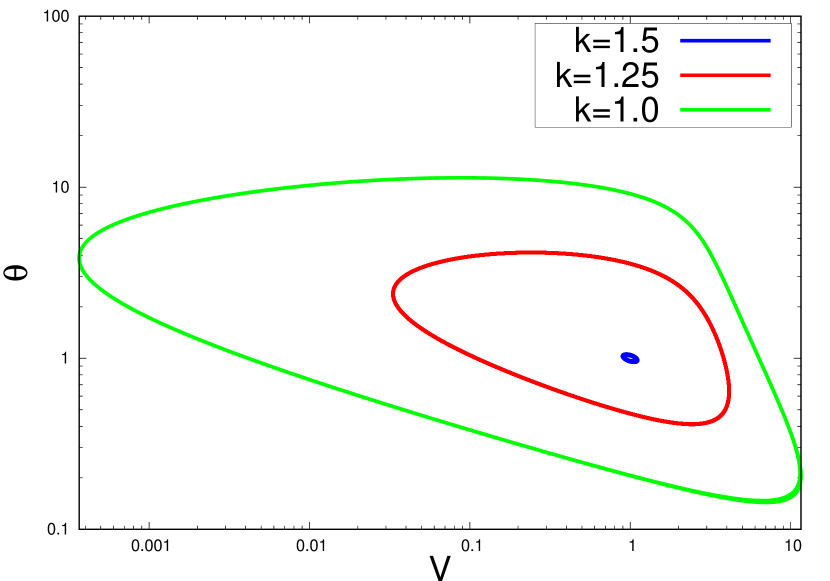
Figure 1: Limit cycles produced by Eqs. (28) and (29). Parameters are set to $n=1/2$, $b=4.0$ and $a=1.0$, so $k_{c}=1.5$. Calculations are conducted for $k=1.5$, $1.25$ and $1.0$.

We also inspect the transient behaviour by considering the velocity step test. Here the velocity is switched between $V_{p}$ and $10V_{p}$. In this case, it is more convenient to use $V_{p}$ in place of an arbitrary constant $V_{0}$ in the RSF, i.e., Eq. (1). We then introduce

$$\delta\mu=\mu-\mu_{0}=a\log V+b\log\theta$$ (33)

with the dimensionless form of the evolution equation.

$$\derivative{\theta}{t}=1-(V\theta)^{n}.\ \ (n>0)$$ (34)

After a steady state is realized at $V_{p}$, we change the velocity to $10V_{p}$. This switch is done instantaneously. We also inspect the opposite case: switch from $10V_{p}$ to $V_{p}$. Such instantaneous switching processes are the ideal limit of infinite stiffness in Eqs. (28) and (29).

As shown in Figure 2, the relaxation after deceleration is generally steeper than that after acceleration. This asymmetric relaxation behaviour is common to the original ageing law, but the asymmetry is rather enhanced as the exponent $n$ decreases from $n=1$. In this respect, modified ageing law I is worse than the original one, although it produces the stable limit cycle.

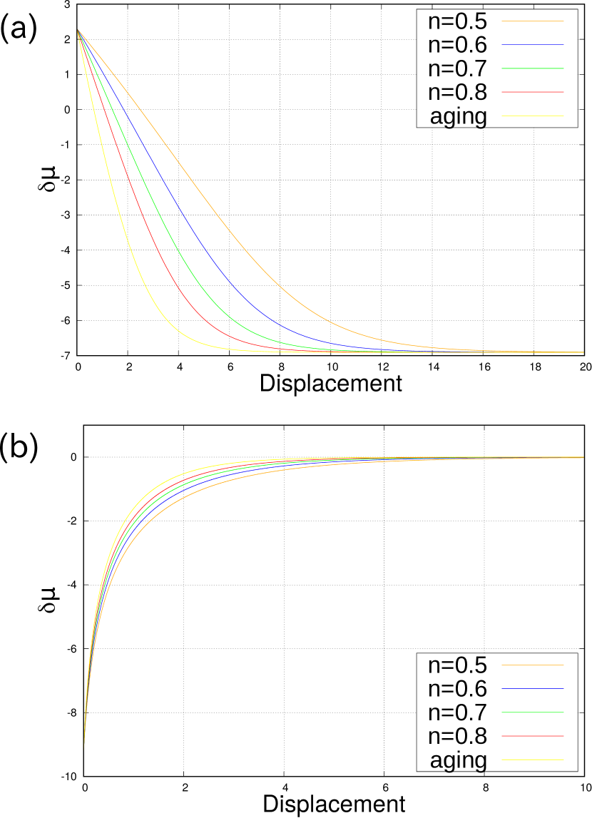
Figure 2: Relaxation of friction coefficient after an abrupt change of the slip velocity for modified ageing law I, calculated from Eqs. (33) and (34) as a function of the (dimensionless) displacement. Parameters are set to $b=4.0$ and $a=1.0$. Effect of the exponent $n$ is studied by setting $n=0.5$, $0.6$, $0.7$, $0.8$, and $1.0$. (a) Velocity is changed from $V=1.0$ to $V=10$. (b) Velocity is changed from $V=10$ to $V=1.0$.

We also perform a slide-hold-slide test (Figures not shown), in which the static friction is measured as a function of the hold time. For $n>1$, this modified aging law predicts the static friction coefficient smaller than the experimental value. This may be expected from the PRZ law case (Perrin et al., 1995; Marone, 1998). For $n<1$, however, the predicted static friction coefficient is only slightly larger than that of the aging law, and therefore the modified aging law predicts the behaviour close to the experimental one.

4.2 Modified ageing law II

As we have seen, it is now possible to avoid the divergence problem with a minor change of the aging law. However, a modified aging law represented by Eq. (34) does not work very well for velocity step experiments. More careful modification is thus needed. Here we propose another evolution equation.

$$\derivative{\hat{\theta}}{\hat{t}}=c+(1-c)\frac{\hat{V}}{V_{c}}-\frac{\hat{V}\hat{\theta}}{L}.$$ (35)

Here $V_{c}$ is a characteristic velocity and $c$ is a constant satisfying $0<c<1$. At steady states, this equation leads to

$$\theta_{\rm ss}=\frac{cL}{V}+(1-c)\frac{L}{V_{c}},$$ (36)

and therefore

$$\mu_{\rm ss}=\mu_{0}+(a-b)\log(\frac{\hat{V}}{V_{0}})+b\log\left[c+(1-c)\frac{\hat{V}}{V_{c}}\right].$$ (37)

This velocity dependence, if $b>a$, is not monotonic as shown in Figure 3. At low velocities, the friction coefficient decreases in a logarithmic manner. This behaviour then changes at a specific velocity

$$\hat{V}=\frac{c}{1-c}\frac{b-a}{a}V_{c},$$ (38)

above which the velocity dependence is positive. A similar crossover is also observed in some experiments (Heslot et al., 1994; Kilgore et al., 1993). The evolution law proposed here thus somehow captures this behaviour.

Note that the parameters in this friction law can be estimated from experiments. Parameters $a$, $b$, and $L$ are estimated in a similar manner with the case of conventional evolution laws. Parameter $c$ should not be close to zero for healing to occur, while the possible range is $0<c<1$. In view of the experimental results by Heslot et al. (1994); Kilgore et al. (1993), the constant $V_{c}$ may be on the order of $1$ to $10$ $\mathrm{[\mu m/s]}$. More detailed discussions are given in Appendix B.

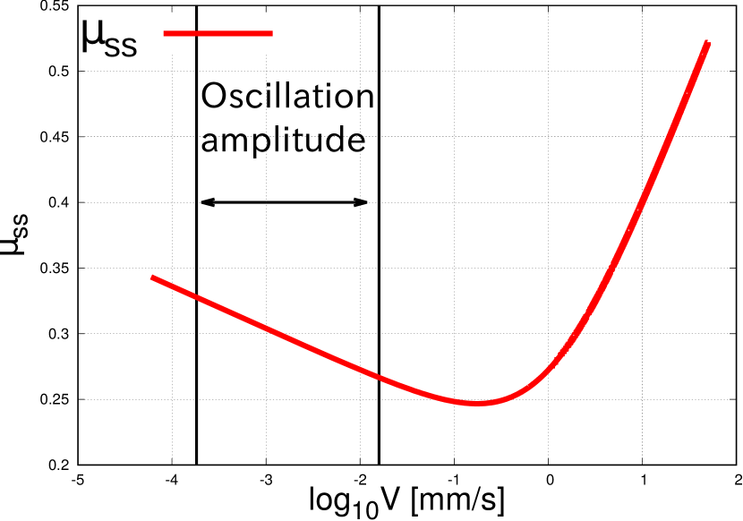
Figure 3: Velocity dependence of steady-state friction coefficient as calculated from the modified ageing law II, Eq. (37). The parameters are set to be $a=0.080$, $b=0.094$, $V_{c}=1.0\mathrm{[mm/s]}$, $c=0.5$, $\mu_{0}=0.369$ and $V_{0}=V_{p}=1.0\mathrm{[\mu m/s]}$. To emphasize that the velocity strengthening branch does not involve, the oscillation amplitude for $k=1.38\times 10^{-2}$ is shown, corresponding to Figure 4.

Applying this law to the single degree of freedom model with dimensionless variables defined by Eq. (8), we get the following equations.

$$\derivative{V}{t}=\frac{k}{a}(1-V)V-\frac{b}{a\theta}[c+(1-c)\alpha V-V\theta]V,$$ (39)

$$\derivative{\theta}{t}=c+(1-c)\alpha V-V\theta.$$ (40)

Here $\alpha\equiv V_{p}/V_{c}$. This system has the fixed point at $(V,\theta)=(1,c+(1-c)\alpha)$. At the point, Jacobi Matrix is

$$J=\left(\begin{array}[]{cc}\displaystyle{\frac{-k}{a}+\frac{bc}{a(c+(1-c)\alpha)}}&\displaystyle{\frac{b}{a}\frac{1}{c+(1-c)\alpha}}\\ -c&-1\end{array}\right)$$ (41)

Calculating the eigenvalues, we get the critical stiffness $k_{c}$ at which the Hopf bifurcation occurs.

$$k_{c}=\frac{(b-a)c-a\alpha(1-c)}{c+(1-c)\alpha}.$$ (42)

The first Lyapunov coefficient of this system is calculated as

$$l_{1}(0)=\frac{(c-1)\alpha b}{2\sqrt{a}[c+\alpha(1-c)]^{3}}\frac{1}{\sqrt{k_{c}}}.$$ (43)

This is always negative since $0<c<1$, and therefore the system undergoes supercritical Hopf bifurcation.

The existence of limit cycle is confirmed numerically as shown in Figure 4, where the amplitude of the limit cycle increases as $k$ decreases. This is a clear evidence for supercritical Hopf bifurcation. We again wish to stress that radiation damping is not introduced here to simulate the limit cycle behaviour.

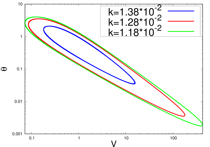
Figure 4: Limit cycles realized by Eqs. (39) and (40). Parameters are set to $a=0.08$, $b=0.094$, $c=0.5$, and $\alpha=0.001$, leading to $k_{c}=2.33$. Calculations are conducted for $k=1.38\times 10^{-2}$, $1.28\times 10^{-2}$ and $1.18\times 10^{-2}$.

We then inspect the response to step-wise change of the slip velocity between $V_{p}$ and $10V_{p}$. Here we use nondimensional variables with (40). Results are shown in Figure 5. To clarify the relaxation behavior, the vertical axis is based on the steady state after relaxation. Although relaxation is not completely symmetric in terms of acceleration and deceleration, the deviation declines at smaller $c$. In short, this evolution law can realize almost the same degree of symmetry as the aging law. Although the symmetry is inferior to the slip law, there is enough rationality in using this law as a substitute for the aging law, considering that there was no evolution law that can realize the limit cycle.

Note also, however, that this result is highly dependent on the parameters value. As can be seen from equation (40), if $\alpha$ is sufficiently small, the form of the equation is almost identical to the aging law, and the similar behavior may appear regardless of the value of c.

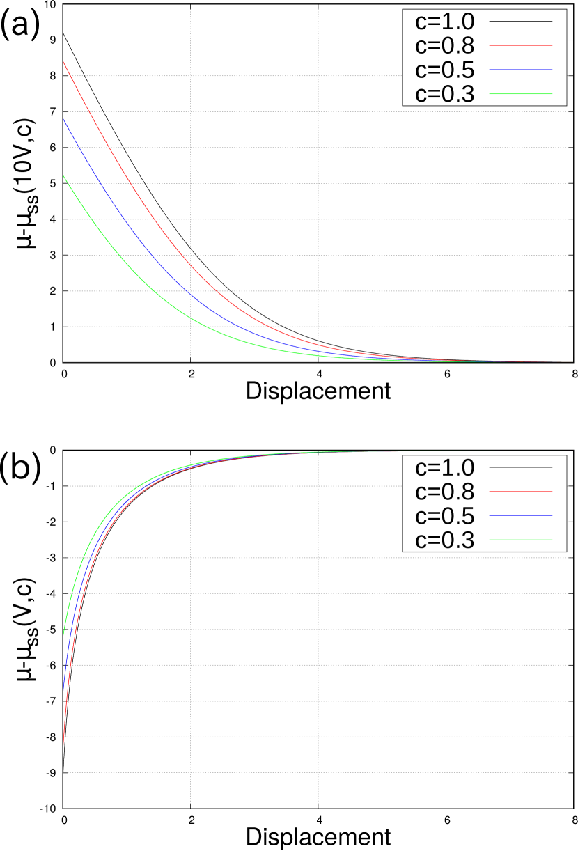
Figure 5: Relaxation of friction coefficient after an abrupt change of the slip velocity for modified ageing law II: Eqs. (33) and (40) with $c=0.8$, $0.5$, and $0.3$. Other parameters are set to be $a=1.0$, $b=4.0$, and $\alpha=0.1$. The vertical axis is set to be zero at the steady state after relaxation. The velocity is changed (a) from $V=1.0$ to $V=10$, (b) from $V=10$ to $V=1.0$.

5 Discussions

5.1 Physical meaning of new evolution law

The evolution law given by Eq. (35) may represent the effect of wear. Friction between brittle materials produces fine wear particles on the sliding interface. Wear particles have the fresh surfaces that possess adhesion force, changing the friction force significantly. However, the adhesion force may be lost due to oxidization of the surface.

Here we assume that the surface of particles can be oxidized to loose the ability for healing, and incorporate this effect into the ageing law. The fraction of the oxidized surface is denoted by $1-c$, where $c$ is the fraction of fresh and unoxidized surface (thus $0<c<1$). The evolution law for the interface is at rest ($V=0$) then reads

$$\derivative{\hat{\theta}}{\hat{t}}=c.$$ (44)

This is interpreted that the ageing is suppressed due to oxidization of the surface.

For sliding surfaces ($V>0$), wear particles are generated with the slip amount. These fresh particles have the unoxidized surface, and thus have the ability for healing. We assume that the oxidized surface is replaced by the fresh surface at the rate of $\hat{V}/V_{c}$, where $V_{c}$ is the characteristic velocity for wear. We thus have the additional ageing term $(1-c)\hat{V}/V_{c}$. Combining these effects with the linear slip weakening term, we obtain Eq. (35).

5.2 Oscillatory motion and velocity dependence of friction

With conventional evolution equations, radiation damping is an essential ingredient to reproduce the periodic oscillation in friction. Since it is similar to linear velocity-strengthening friction, one might regard the velocity-strengthening nature is essential (Matsuzawa et al., 2010; Shibazaki & Shimamoto, 2007; Barbot, 2019a). However, we wish to stress that the velocity-strengthening friction is not essential to reproduce the periodic oscillation. This is obvious because Eq. (27), which is velocity-weakening, reproduces the limit cycle.

Similarly, another evolution equation, Eq. (35), changes its velocity dependence from negative to positive (from velocity weakening to velocity-strengthening) at the crossover velocity given by Eq. (38). However, we wish to stress that the limit cycle behaviour is not due to this crossover, because the velocity oscillates around $V_{p}$ and does not necessarily exceed the crossover velocity. In other words, the friction is always velocity-weakening during the oscillatory motion. The oscillatory motion is thus not due to the non-monotonic nature of the velocity dependence of friction. To illustrate this point more clearly, the velocity range of the limit cycle oscillation is shown in Figure 3.

5.3 Relevance to slow slip events

Recent development of observation technology enables us to discover various kinds of slow earthquakes (Obara & Kato, 2016), which span a wide range of time and energy scales (Ide et al., 2007). This implies that the natural fault motion is much more complex than a simple stick-slip motion. A remarkable case is off coast of Tohoku, Japan, where the subduction rate oscillates with the period of several years (Uchida et al., 2016). The maximum subduction rate during an oscillation period is only several times larger than the average subduction rate, and therefore this oscillation may be interpreted as a family of slow slip events (SSE).

Here we wish to discuss SSE based on the present fault-patch model with the RSF. This simple model may be partly verified by observations that SSEs repeat themselves in patch-like regions. The use of RSF may be rational in view of small slip rates of SSE. Here we estimate the oscillation period using our new evolution equation, Eq. (35). Linear stability analysis leads to the expression for the oscillation period, $T_{2}$.

$$T_{2}=2\pi\frac{L}{V_{p}}\sqrt{\frac{a(c+(1-c)\alpha)}{(b-a)c-a\alpha(1-c)}},$$ (45)

where $\alpha=V_{p}/V_{c}$. In a similar manner, the oscillation period for the aging law and the slip law is calculated as

$$T_{1}=2\pi\frac{L}{V_{p}}\sqrt{\frac{a}{b-a}}.$$ (46)

The ratio is

$$\frac{T_{2}}{T_{1}}=\sqrt{1+\frac{b\alpha(1-c)}{(b-a)c-a\alpha(1-c)}}.$$ (47)

Recalling the critical spring constant $k_{c}$ given by Eq. (42), $(b-a)c>a\alpha(1-c)$ must hold since $k_{c}$ must be positive. It thus follows that $T_{2}/T_{1}>1$, meaning that a new evolution equation gives a longer period than the slip law or the ageing law.

To estimate the period $T_{1}$ and $T_{2}$ for subduction zones, numerical values are required for $a$, $b$, $V_{p}$, and $L$. Precise estimate of these parameters for natural faults are difficult and there has been no agreement to date. We thus limit ourselves to a crude guess. The length constant $L$ has been estimated as several millimeters via the geodetic inversion on the afterslip data for the 2003 Tokachi-oki earthquake (Fukuda et al., 2009). We thus assume $L$ to be a millimeter here. The subduction velocity $V_{p}$ may be of the order of $\mathrm{[cm/year]}$. We assume it as several nanometers per second. Then $L/V_{p}$ is on the order of $10^{6}$ s. If we assume that $a$ and $b$ are on the order of $10^{-2}$ in view of typical experiments, $T_{2}$ is estimated as a few years, whereas $T_{1}$ is several months. In this respect, $T_{2}$ is more appropriate for the period of SSE cycles. Namely, the new evolution equation proposed here may be more suitable in explaining a period of several years for SSE. The period $T_{1}$ can be a few years if $b/a-1$ is as small as $10^{-3}$, but such a condition requires finer tuning of the parameters $a$ and $b$.

At the same time, however, we need to recall that the oscillation period estimated here is based on a simple fault-patch model. Subduction zones, where most slow earthquakes occur, extend over several hundred kilometers and involve many kinds of heterogeneity. If there is a slip patch that is sufficiently isolated from other seismogenic zones, the discussion here may apply. Otherwise, the discussion here should be interpreted as an ideal case analysis.

Since the observed oscillation of subduction rates is spatially heterogeneous (Uchida et al., 2016), the discussion given here should be interpreted as a preliminary guess for more quantitative studies on spatially extended systems, which would be a promising attempts in the future.

5.4 Case of multiplicative form

The discussions so far are based on the standard form of RSF, in which the effects of slip rate and state variable(s) are expressed in the additive manner. On the other hand, an alternative form is also known, in which the effects of slip rate and state variable(s) are expressed in the multiplicative manner. We may discuss the stability of limit cycle produced by this alternative form of RSF.

We inspect two variations proposed by Barbot (2019b) and Bar-Sinai et al. (2014), respectively, by performing numerical calculations on the patch model together with the standard ageing law. We find the stable limit cycle without radiation damping for both the cases. Details of the results are given in the supplementary material. This result indicates the supremacy of the multiplicative form for the RSF law in reproducing the stable limit cycle. One may thus need to reflect on the use of popular additive form of the RSF, depending on the specific situation that one needs to consider.

6 Conclusions

In a slip patch model implemented with the rate and state friction (RSF) law, it has been well known that the numerical solution diverges unless the radiation damping is introduced. However, this divergence has been known only empirically and numerically. Here we have analytically shown that the divergence is inevitable for three major evolution equations: the slip law, the ageing law, and the Nagata’s law.

The radiation damping, which has been conventionally used, is due to the energy dissipation caused by the radiation of elastic waves. Therefore, from a physical point of view, introducing radiation damping may not be verified in models for slow aseismic motion such as slow slip events, in which seismic waves are not radiated. On the other hand, slow slip events are often accompanied by tremors, which radiate weak seismic waves. Such a complex nature of slow earthquakes may verify the use of radiation damping, but the quantitative aspect is not clear.

In light of the above points, the choice of evolution equation requires discretion in modelling slow earthquakes, which radiate only a little amount of seismic waves. To model slow aseismic slip motion, two new evolution laws are proposed here. Both the equations reproduce slow periodic oscillation (i.e., the limit cycle) without radiation damping, at least for a single degree-of-freedom system. Modified ageing law I illustrates that a limit cycle can be realized only with a minor change in the evolution law. However, in view of the asymmetric relaxation after the abrupt velocity change, it cannot be a good replacement for the existing evolution laws. Modified ageing law II also exhibits asymmetric relaxation, but it is at the same level as the original ageing law. The only defect may be time-dependent healing is somewhat (by factor $c$) smaller than the original ageing law, but the difference is as small as $b\log c$. This is generally negligible.

The difference between the two novel equations is most apparent in the steady-state behaviours. The velocity dependence of modified ageing law I is monotonic, whereas the modified ageing law II exhibits crossover to velocity-strengthening above a certain slip velocity. The difference may be useful in determining a suitable evolution law based on the experimental data. Regarding a relaxation behavior after an abrupt change of the slip velocity, the modified ageing law II is more consistent with experiments than the modified ageing law I.

Since this study is limited to a single degree of freedom system, application of these new evolution laws to spatially extended systems may be promising future work toward understanding of slow earthquakes. At the same time, critical consideration on the use of additive form of the RSF is needed.

Data Availability Statements

Simulation codes are available upon request.

Appendix A Normal form theory

To know the type of bifurcation, we must calculate the nonlinear effect directly. Normal form theory is an effective way for this purpose. Here we consider a 2D dynamical system that undergoes Hopf bifurcation. According to the theory, after appropriate coordinate transformation, one can rewrite the time evolution equation as follows. in the neighbourhood of the bifurcation point,

$$\derivative{u}{t}=(\beta+i)u+\sigma_{1}u\absolutevalue{u}^{2}+\order{\absolutevalue{u^{4}}},$$ (48)

where $u$ is a complex variable, $\beta$ is a constant, and $\sigma_{1}=\pm 1$ corresponding to the the sign of the first Lyapunov coefficient, $l_{1}(0)$. The functional form of $l_{1}(0)$ is not shown here. One can refer to a reference (Kuznetsov, 2004) or supplemental material.

The type of Hopf bifurcation, either supercritical or subcritical, is determined by $\sigma_{1}$. When $\sigma_{1}=-1$, the system undergoes supercritical Hopf bifurcation. In this case, the limit cycle of small amplitude arises once the system loses its stability. If $\sigma_{1}=1$, subcritical Hopf bifurcation occurs. Then the limit cycle appears with the large amplitude. In general, the solution diverges once the system loses its stability.

There are some methods to calculate the value of $l_{1}(0)$ numerically. In this paper, we employ the method stated in (Kuznetsov, 2004) using a software, Maple^TM. Detailed calculation is shown in supplement material.

Appendix B Determining the parameters for modified aging law II

The parameters in modified aging law II can be determined from experimental data. Noting that $\mu_{0}$ and $V_{0}$ are arbitrary constants, the parameters to be determined are $a,b,c,V_{c}$ and $L$.

1. Parameter $a$
   This is determined from the direct effect in the velocity step experiment, as is usually done for major evolution laws. For sudden velocity change, the state variable does not change and the change of friction coefficient $\delta\mu$ is written as

   $$\delta\mu=a\log(\frac{V_{2}}{V_{1}}),$$ (49)

   where the slip velocity is changed from $V_{1}$ to $V_{2}$.

2. Parameter $b$
   Parameter $b$ involves the healing (Beeler et al., 1994; Marone, 1998). If holding time is sufficiently long and the apparatus is sufficiently stiff, the velocity can be regarded to be zero during the holding time. Then the state variable evolves as

   $$\derivative{\hat{\theta}}{\hat{t}}=c.$$ (50)

   Then, as in the case of original aging law, the amount of the healing of the friction $\Delta\mu$ depends on the holding time as

   $$\derivative{\Delta\mu}{\log\hat{t}}\simeq b,$$ (51)

   from which parameter $b$ is determined.

3. Parameters $c$ and $V_{c}$
   These parameters are determined from the crossover velocity $\hat{V}_{\rm cross}$ and the value of the friction coefficient there:

   $$\hat{V}_{\rm cross}=\frac{c}{1-c}\frac{b-a}{a}V_{c},$$ (52)

   above which the velocity dependence switches from negative to positive. The steady-state friction coefficient at the crossover velocity is

   $$\mu_{\rm ss}=\mu_{0}+(a-b)\log(\frac{{\hat{V}}_{\rm cross}}{V_{0}})+b\log(\frac{b}{a})+b\log c.$$ (53)

   Since ${\hat{V}}_{\rm cross}$ can be known from experiment, $c$ and $V_{c}$ are found using Eqs. (52) and (53).

4. Parameter $L$
   This is determined from the relaxation process in velocity step tests by comparing the model behaviour with the observed relaxation process.

.

References

- Bar-Sinai et al. (2014) Bar-Sinai, Y., Spatschek, R., Brener, E. A., & Bouchbinder, E., 2014. On the velocity-strengthening behavior of dry friction, Journal of Geophysical Research: Solid Earth, 119(3), 1738–1748.
- Barbot (2019a) Barbot, S., 2019a. Slow-slip, slow earthquakes, period-two cycles, full and partial ruptures, and deterministic chaos in a single asperity fault, Tectonophysics, 768, 228171.
- Barbot (2019b) Barbot, S., 2019b. Modulation of fault strength during the seismic cycle by grain-size evolution around contact junctions, Tectonophysics, 765, 129–145.
- Beeler et al. (1994) Beeler, N. M., Tullis, T. E., & Weeks, J. D., 1994. The roles of time and displacement in the evolution effect in rock friction, Geophysical Research Letters, 21(18), 1987–1990.
- Bizzarri (2011) Bizzarri, A., 2011. On the deterministic description of earthquakes, Reviews of Geophysics, 49(3).
- Cochard & Madariaga (1994) Cochard, A. & Madariaga, R., 1994. Dynamic faulting under rate-dependent friction, pure and applied geophysics, 142(3), 419–445.
- Dieterich (1979) Dieterich, J. H., 1979. Modeling of rock friction: 1. experimental results and constitutive equations, Journal of Geophysical Research: Solid Earth, 84(B5), 2161–2168.
- Fukuda et al. (2009) Fukuda, J., Johnson, K. M., Larson, K. M., & Miyazaki, S., 2009. Fault friction parameters inferred from the early stages of afterslip following the 2003 tokachi-oki earthquake, Journal of Geophysical Research: Solid Earth, 114(B4).
- Gu et al. (1984) Gu, J.-C., Rice, J. R., Ruina, A. L., & Tse, S. T., 1984. Slip motion and stability of a single degree of freedom elastic system with rate and state dependent friction, Journal of the Mechanics and Physics of Solids, 32(3), 167–196.
- Hawthorne & Rubin (2013) Hawthorne, J. C. & Rubin, A. M., 2013. Laterally propagating slow slip events in a rate and state friction model with a velocity-weakening to velocity-strengthening transition, Journal of Geophysical Research: Solid Earth, 118(7), 3785–3808.
- Heslot et al. (1994) Heslot, F., Baumberger, T., Perrin, B., Caroli, B., & Caroli, C., 1994. Creep, stick-slip, and dry-friction dynamics: Experiments and a heuristic model, Phys. Rev. E, 49, 4973–4988.
- Ide et al. (2007) Ide, S., Beroza, G. C., Shelly, D. R., & Uchide, T., 2007. A scaling law for slow earthquakes, Nature, 447(7140), 76–79.
- Kilgore et al. (1993) Kilgore, B. D., Blanpied, M. L., & Dieterich, J. H., 1993. Velocity dependent friction of granite over a wide range of conditions, Geophysical Research Letters, 20(10), 903–906.
- Kuznetsov (2004) Kuznetsov, Y. A., 2004. Elements of applied bifurcation theory, Springer-Verlag New York.
- Marone (1998) Marone, C., 1998. Laboratory-derived friction laws and their application to seismic faulting, Annual Review of Earth and Planetary Sciences, 26(1), 643–696.
- Matsuzawa et al. (2010) Matsuzawa, T., Hirose, H., Shibazaki, B., & Obara, K., 2010. Modeling short- and long-term slow slip events in the seismic cycles of large subduction earthquakes, Journal of Geophysical Research: Solid Earth, 115(B12).
- Nagata et al. (2012) Nagata, K., Nakatani, M., & Yoshida, S., 2012. A revised rate- and state-dependent friction law obtained by constraining constitutive and evolution laws separately with laboratory data, Journal of Geophysical Research: Solid Earth, 117(B2).
- Obara & Kato (2016) Obara, K. & Kato, A., 2016. Connecting slow earthquakes to huge earthquakes, Science, 353(6296), 253–257.
- Perrin et al. (1995) Perrin, G., Rice, J. R., & Zheng, G., 1995. Self-healing slip pulse on a frictional surface, Journal of the Mechanics and Physics of Solids, 43(9), 1461–1495.
- Ranjith & Rice (1999) Ranjith, K. & Rice, J., 1999. Stability of quasi-static slip in a single degree of freedom elastic system with rate and state dependent friction, Journal of the Mechanics and Physics of Solids, 47(6), 1207–1218.
- Rice & Ruina (1983) Rice, J. & Ruina, A., 1983. Stability of steady frictional slipping, Journal of Applied Mechanics-transactions of The Asme - J APPL MECH, 50, 343–349.
- Rice (1993) Rice, J. R., 1993. Spatio-temporal complexity of slip on a fault, Journal of Geophysical Research: Solid Earth, 98(B6), 9885–9907.
- Rice et al. (2001) Rice, J. R., Lapusta, N., & Ranjith, K., 2001. Rate and state dependent friction and the stability of sliding between elastically deformable solids, Journal of the Mechanics and Physics of Solids, 49(9), 1865–1898, The JW Hutchinson and JR Rice 60th Anniversary Issue.
- Ruina (1983) Ruina, A., 1983. Slip instability and state variable friction laws, Journal of Geophysical Research: Solid Earth, 88(B12), 10359–10370.
- Scholz (1990) Scholz, C. H., 1990. The mechanics of earthquakes and faulting, Cambridge university press.
- Shibazaki & Shimamoto (2007) Shibazaki, B. & Shimamoto, T., 2007. Modelling of short-interval silent slip events in deeper subduction interfaces considering the frictional properties at the unstable?stable transition regime, Geophysical Journal International, 171(1), 191–205.
- Strogatz (2001) Strogatz, S. H., 2001. Nonlinear Dynamics And Chaos: With Applications To Physics, Biology, Chemistry, And Engineering (Studies in Nonlinearity), CRC Press.
- Sugiura et al. (2014) Sugiura, N., Hori, T., & Kawamura, Y., 2014. Synchronization of coupled stick-slip oscillators, Nonlinear Processes in Geophysics, 21(1), 251–267.
- Uchida et al. (2016) Uchida, N., Iinuma, T., Nadeau, R. M., Bürgmann, R., & Hino, R., 2016. Periodic slow slip triggers megathrust zone earthquakes in northeastern japan, Science, 351(6272), 488–492.
- Viesca (2016a) Viesca, R. C., 2016a. Self-similar slip instability on interfaces with rate- and state-dependent friction, Proceedings of the Royal Society A: Mathematical, Physical and Engineering Sciences, 472(2192), 20160254.
- Viesca (2016b) Viesca, R. C., 2016b. Stable and unstable development of an interfacial sliding instability, Phys. Rev. E, 93, 060202.