Dual-Octave Convolution for Accelerated Parallel MR Image Reconstruction

Abstract

Magnetic resonance (MR) image acquisition is an inherently prolonged process, whose acceleration by obtaining multiple undersampled images simultaneously through parallel imaging has always been the subject of research. In this paper, we propose the Dual-Octave Convolution (Dual-OctConv), which is capable of learning multi-scale spatial-frequency features from both real and imaginary components, for fast parallel MR image reconstruction. By reformulating the complex operations using octave convolutions, our model shows a strong ability to capture richer representations of MR images, while at the same time greatly reducing the spatial redundancy. More specifically, the input feature maps and convolutional kernels are first split into two components (i.e., real and imaginary), which are then divided into four groups according to their spatial frequencies. Then, our Dual-OctConv conducts intra-group information updating and inter-group information exchange to aggregate the contextual information across different groups. Our framework provides two appealing benefits: (i) it encourages interactions between real and imaginary components at various spatial frequencies to achieve richer representational capacity, and (ii) it enlarges the receptive field by learning multiple spatial-frequency features of both the real and imaginary components. We evaluate the performance of the proposed model on the acceleration of multi-coil MR image reconstruction. Extensive experiments are conducted on an in vivo knee dataset under different undersampling patterns and acceleration factors. The experimental results demonstrate the superiority of our model in accelerated parallel MR image reconstruction. Our code is available at: github.com/chunmeifeng/Dual-OctConv.

Introduction

Magnetic resonance (MR) imaging has become increasingly popular in radiology and medicine over the past decade, thanks to its advantages of being non-radiative, having a high spatial-resolution, and providing superior soft tissue contrast (Sun et al. 2018). However, a major limitation of MR imaging is that it requires a much longer acquisition time than other imaging techniques, e.g., computed tomography (CT), X-Ray, and ultrasound (Wang et al. 2020). Recently, great efforts have been devoted to accelerated MR image reconstruction, which is typically achieved by reconstructing the desired full images from undersampled measured data (Aggarwal, Mani, and Jacob 2018).

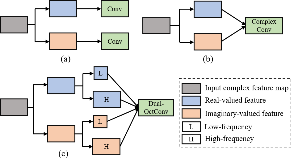
Figure 1: Previous methods utilize vanilla convolutions (a) to process the real- and imaginary-valued parts of an MR image independently or complex convolutions (b) to jointly deal with the two parts. In contrast, we propose Dual-OctConv, which is a generalization of complex convolutions, to process complex-valued inputs in a multi-frequency space for more effective feature representations.

Parallel MR imaging is considered as one of the most important achievements in accelerated MR imaging (Knoll et al. 2019; Wang et al. 2017). Most studies (e.g., SENSE (Pruessmann et al. 1999), GRAPPA (Griswold et al. 2002), SPIRiT (Lustig and Pauly 2010)) take advantage of spatial sensitivity and gradient coding to reduce the amount of data required for reconstruction, thereby shortening the imaging time. Moreover, compressed sensing (CS) is an important technique for fast MR image reconstruction (Feng et al. 2019), which recovers the desired signal from $k$-space data sampled below the Nyquist rate. Typical CS-based approaches adopt a sparsity prior (Liu et al. 2019), low-rank sparse sampling (He et al. 2016; Haldar and Zhuo 2016), or manifold learning (Nakarmi et al. 2017) for reconstruction.

More recently, with the renaissance of deep neural networks, deep learning techniques (Zhou et al. 2021; Feng et al. 2021), especially convolutional neural networks (CNNs), have been widely used for parallel MR imaging (Ramani and Fessler 2010; Haldar and Zhuo 2016). Since models are trained offline over large-scale data, only a few extra online samples are required for reconstruction. The model-based unrolling methods (Hammernik et al. 2018; Chen et al. 2019b) combine mathematical structures (e.g., variational inference, compressed sensing) with deep learning for fast MR image reconstruction. Moreover, extensive approaches (Kwon, Kim, and Park 2017; Schlemper et al. 2019b, a; Sriram et al. 2020; Wang et al. 2020) propose end-to-end learnable models to remove the aliasing artifacts from images that are reconstructed from undersampled multi-coil $k$-space data. The mapping between a zero-filled $k$-space and fully-sampled MR image is automatically learned by CNNs, requiring no sub-problem division.

Most of the above approaches directly borrow vanilla convolutions used in standard CNNs for $k$-space data in MR image reconstruction. However, vanilla convolutions are designed for real-valued natural images, and cannot deal with complex-valued inputs. To solve this, early studies (Wang et al. 2016) simply discarded the imaginary part or processed the real and imaginary parts independently for real-valued convolutions (see Fig. 1(a)). To avoid information loss, complex convolution (Trabelsi et al. 2018) has recently been proposed to process complex-valued inputs and encourages information exchange between real and imaginary values (see Fig. 1(b)). Though impressive, existing complex convolution operations ignore the intrinsic multi-frequency property of MR images, leading to limited single-scale contextual information and high spatial redundancy in final representations.

To address these limitations, we take a further step towards exploring multi-frequency representation learning in parallel MR image reconstrucion (see Fig. 1(c)). We propose a novel Dual-Octave Convolution (Dual-OctConv), which enables our model to learn multi-frequency representations of multi-coil MR images (Chen et al. 2019a). Unlike complex convolutions, our Dual-OctConv processes the real (or imaginary) part of MR image features by factorizing it into high- and low-frequency components. The low-frequency component shares information across neighboring locations, and can thus be efficiently processed in low-resolution to enlarge the receptive field and reduce the spatial redundancy. Finally, we combine the features of the real and imaginary parts for reconstruction. Benefiting from Dual-OctConv, our model has a more powerful capability in multi-scale representation learning, and can thus better capture soft tissues (e.g., vascular, muscles) with varying sizes and shapes.

Our main contributions are three-fold: First, we propose multi-frequency feature representations for accelerated parallel MR image reconstruction, and demonstrate their ability to capture multi-scale contextual information. Second, we devise the Dual-OctConv to deal with complex-valued inputs in a multi-frequency representation space, and encourages information exchange across various frequency domains. The Dual-OctConv is a generalization of the standard complex convolution, and endows our model several appealing characteristics (e.g., larger receptive field, higher flexibility, and computationally more efficient). Third, our model shows significant performance improvements against state-of-the-art algorithms on an in vivo knee dataset.

Related Work

Deep Learning in MR image reconstruction. Ever since the pioneering works introducing CNNs for computer vision tasks, such as image classification and face recognition, researchers have made substantial efforts to improve medical and clinical practice using deep learning techniques. (Wang et al. 2016) proposed the first deep learning based MR image reconstruction framework, which learns the mapping between fully-sampled single-coil MR images and their counterpart data reconstructed from a zero-filled undersampled $k$-space. A large number of networks were then developed for MR image reconstruction, especially non-parallel reconstruction (Sun et al. 2019). For example, (Yang et al. 2020) proposed a model-based unrolling method, which formulates the algorithm within a deep neural network, and trained the network with a small amount of data. (Han et al. 2018) employed U-Net to model a domain adaptation structure that removes aliasing artifacts from corrupted images. Similar works have also used deep residual networks (Lee et al. 2018), recursive dilated network (Sun et al. 2018), and Generative Adversarial Network (Quan, Nguyen-Duc, and Jeong 2018; Yang et al. 2017) to restore high-resolution MR images from undersampled $k$-space data.

In parallel imaging, one representative network is the variational network (VN-Net) (Hammernik et al. 2018), which combines the mathematical structure of the variational model with deep learning for fast multi-coil MR image reconstruction. Another model-based deep framework (Chen et al. 2019b) was designed with a split Bregman iterative algorithm to achieve accurate reconstruction from multi-coil undersampled $k$-space data. To obtain high-fidelity reconstructions, GrappaNet (Sriram et al. 2020) was proposed to combine traditional parallel imaging methods with deep neural networks. Recently, complex-valued representations have demonstrated superiority in processing complex-valued inputs (Trabelsi et al. 2018). For example, Wang et al. (2020) applied complex convolutions to jointly process real and imaginary values for comprehensive feature representations. In contrast, our approach represents complex-valued input features in a multi-frequency space. The Dual-OctConv, proposed for processing such multi-frequency data, can capture richer contextual knowledge, leading to significant improvement in performance.

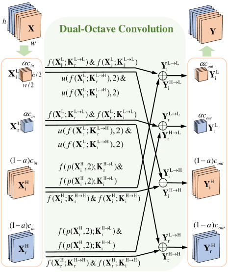
Figure 2: Detailed design of our Dual-OctConv. $\mathbf{X}\!\in\!\mathbb{C}^{c\!\times\!h\!\times\!w}$ represents the input complex-valued feature maps, and $\mathbf{Y}\!\in\!\mathbb{C}^{c\!\times\!h\!\times\!w}$ indicates the corresponding output feature maps, modulated by the Dual-OctConv. $u$ and $p$ denote the upsampling and average pooling operations, respectively. Please see Eq. (5) for more details.

Multi-Scale Representation Learning. Multi-scale information has proven effective in various computer vision tasks (e.g., image classification, object detection, semantic segmentation). Several strategies have been proposed for multi-scale representation learning, yielding significant performance improvement in a number of tasks. For example, Ke, Maire, and Yu (2017) proposed a multi-grid network to propagate and integrate information across multiple scales for image classification. Multi-scale information has also been proven effective in restoring image details for image enhancement (Nah, Hyun Kim, and Mu Lee 2017; Ren et al. 2016; Li et al. 2018). In addition, various well-known techniques (e.g., FPN (Lin et al. 2017) and PSP (Zhao et al. 2017)) have been proposed for learning multi-scale representations in object detection and segmentation tasks (Zhou et al. 2020b, a). Recently, the Octave convolution (Chen et al. 2019a) was proposed to learn multi-scale features based on the spatial frequency model, greatly improving performance in natural image and video recognition.

In this work, we demonstrate the appealing properties of the Octave convolution for accelerated parallel MR image reconstruction, which helps to capture multi-scale information from multiple spatial-frequency features. Based on this, we propose a novel Dual-OctConv for accelerated parallel MR image reconstruction, which enables our model to capture details of vasculatures and tissues with varying sizes and shapes, yielding high-fidelity reconstructions.

Methodology

Problem Formulation

MR scanners acquire $k$-space data through the receiver coils and then utilize an inverse multidimensional Fourier transform to obtain the final MR images. In parallel imaging, multiple receiver coils are used to simultaneously acquire $k$-space data from the target under scanning.

Let $\mathbf{A}\!=\!\mathbf{M}\!\mathbf{F}\!\in\!\mathbb{C}^{M\times N}$ denote the undersampled Fourier encoding matrix, where $\mathbf{F}$ is the multidimensional Fourier transform, and $\mathbf{M}$ is an undersampled mask operator. In parallel imaging, the same mask is used for all coils. The undersampled $k$-space data from each coil can be expressed as

$$\mathbf{y}_{i}=\mathbf{A}(\mathbf{S}_{i}\mathbf{x}),$$ (1)

where $i=1,2,...,c$, with $c$ denoting the number of coils, $\mathbf{x}\!\in\!\mathbb{C}^{N\times 1}$ is the ground truth MR image, $\mathbf{y}_{i}\!\in\!\mathbb{C}^{M\times 1}(M\!<\!<\!N)$ is the undersampled $k$-space data for the $i$-th coil, and $\mathbf{S}_{i}$ is a complex-valued diagonal matrix encoding the sensitivity map of the $i$-th coil. The coil sensitivities modulate the $k$-space data, which is measured by each coil. The coil configuration and interactions with the anatomical structures under scanning can affect coil sensitivities, so $\mathbf{S}_{i}$ changes across different scans. In addition, the obtained image will contain aliasing artifacts, if the inverse Fourier transform is directly applied to undersampled $k$-space data.

We can reconstruct $\hat{\mathbf{x}}$ with prior knowledge of its properties, which is formulated as the following problem:

$$\hat{\mathbf{x}}=\mathop{\arg\min}_{\mathbf{x}}\sum_{i=1}^{c}\ \|{\mathbf{y}_{i}-\mathbf{A}(\mathbf{S}_{i}\mathbf{x})}\|^{2}_{2}+\ \lambda\Psi(\mathbf{x}),$$ (2)

where $\Psi$ is a regularization function and $\lambda$ controls the trade-off between the two terms.

The problem presented in Eq. (2) can be effectively resolved using CNNs, which avoids time-consuming numerical optimization and the need of a coil sensitivity map. During training, we update the network weights as follows:

$$\hat{\boldsymbol{\theta}}=\mathop{\min}_{\boldsymbol{\theta}}\frac{1}{N}\sum_{n=1}^{N}\|{\mathbf{x^{\prime}}(n)-f_{\boldsymbol{\theta}}(\mathbf{y^{\prime}}(n))}\|_{1},$$ (3)

where $\mathbf{y^{\prime}}(n)$ is the $n$-th multi-channel image obtained from the zero-filled $k$-space data, $\mathbf{x^{\prime}}(n)$ is the $n$-th ground truth multi-channel image, $N$ is the total number of training samples, and $f_{\boldsymbol{\theta}}(\cdot)$ is an end-to-end mapping function parameterized by $\boldsymbol{\theta}$, which contains a large number of adjustable network weights. Training with Eq. (3) can reconstruct the expected MR images, but the original information of the data acquired in the $k$-space cannot be well preserved. If we incorporate the undersampled $k$-space data into the data fidelity at the training stage, the network can yield improved reconstruction results. For this purpose, we add the data fidelity units in our network, as in (Wang et al. 2020). After the network is trained, we obtain a set of optimal parameters $\boldsymbol{\hat{\theta}}$ for the reconstruction of multi-channel image, and predict the multi-channel image via $\mathbf{\hat{x}^{\prime}}=f_{\hat{\boldsymbol{\theta}}}(\mathbf{y^{\prime}})$. Finally, we use an adaptive coil combination method (Wang et al. 2020) to obtain the expected MR image from $\mathbf{\hat{x}^{\prime}}$.

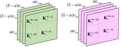
Figure 3: The Dual-OctConv kernels. Green and pink squares denotes the imaginary and real kernels, respectively.

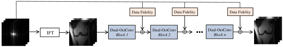
Figure 4: Architecture of our network for parallel MR image reconstruction. The input is a set of zero-filled multi-coil $k$-space measurements, while the output is the reconstructed multi-channel MR image. $\rm IFT$ represents the 2D inverse Fourier transform.

Dual-Octave Convolution

To obtain rich multi-scale context information, we first represent the multi-channel input with complex filters, and then decompose it into low and high spatial frequency parts. Let $\mathbf{X}\!\in\!\mathbb{C}^{c\times h\times w}$ be the the complex feature maps with $c$, $h$, and $w$ denoting the number of channels, height, and width, respectively. As illustrated in Fig. 2, we convolve $\mathbf{X}=\mathbf{X}_{\rm r}+i\mathbf{X}_{\rm i}$ with a complex filter matrix $\mathbf{K}=\mathbf{K}_{\rm r}+i\mathbf{K}_{\rm i}$. Mathematically, we have

$${\left[\begin{array}[]{ccc}\Re(\mathbf{K}*\mathbf{X})\\ \Im(\mathbf{K}*\mathbf{X})\end{array}\right]}={\left[\begin{array}[]{ccc}\mathbf{K}_{\rm r}&-\mathbf{K}_{\rm i}\\ \mathbf{K}_{\rm i}&\mathbf{K}_{\rm r}\end{array}\right]}*{\left[\begin{array}[]{ccc}\mathbf{X}_{\rm r}\\ \mathbf{X}_{\rm i}\end{array}\right]},$$ (4)

where the matrices $\mathbf{K}_{\rm r}$ and $\mathbf{K}_{\rm i}$ represent real and imaginary kernels, and vectors $\mathbf{X}_{\rm r}$ and $\mathbf{X}_{\rm i}$ represent real and imaginary feature maps. Note that all the kernels and feature maps are expressed by real matrices since the complex arithmetics are simulated by real-valued entities.

To effectively fuse the real and imaginary parts of data (i.e., $\mathbf{X}_{\rm r}$ and $\mathbf{X}_{\rm i}$), we split them into low and high spatial frequency groups $\mathbf{X}_{\rm r}=\left\{\mathbf{X}_{\rm r}^{\rm L},\mathbf{X}_{\rm r}^{\rm H}\right\}$, $\mathbf{X}_{\rm i}=\left\{{\mathbf{X}_{\rm i}^{\rm L},\mathbf{X}_{\rm i}^{\rm H}}\right\}$, where $\mathbf{X}^{\rm H}\!\in\!\mathbb{C}^{(1-\alpha)c\times h\times w}$ capture the high-frequency fine details of the data and $\mathbf{X}^{\rm L}\!\in\!\mathbb{C}^{\alpha c\times 0.5h\times 0.5w}$ determine the low-frequency image contrast. Here, $\alpha\!\in\![0,1]$ controls the ratio of channels that are allocated to low-frequency and high-frequency feature maps. Note that the Dual-OctConv will turn into the standard complex convolution (Trabelsi et al. 2018) when $\alpha\!=\!0$. As shown in Fig. 3, the complex filter matrix is further expressed as $\mathbf{K}_{\rm r}^{\rm H}=\left[\mathbf{K}_{\rm r}^{{\rm H}\rightarrow{\rm L}},\mathbf{K}_{\rm r}^{{\rm H}\rightarrow{\rm H}}\right]$, $\mathbf{K}_{\rm i}^{\rm H}=\left[\mathbf{K}_{\rm i}^{{\rm H}\rightarrow{\rm L}},\mathbf{K}_{\rm i}^{{\rm H}\rightarrow{\rm H}}\right]$, $\mathbf{K}_{\rm r}^{\rm L}=\left[\mathbf{K}_{\rm r}^{{\rm L}\rightarrow{\rm H}},\mathbf{K}_{\rm r}^{{\rm L}\rightarrow{\rm L}}\right]$, $\mathbf{K}_{\rm i}^{\rm L}=\left[\mathbf{K}_{\rm i}^{{\rm L}\rightarrow{\rm H}},\mathbf{K}_{\rm i}^{{\rm L}\rightarrow{\rm L}}\right]$ to convolve with $\mathbf{X}_{\rm r}^{\rm L}$, $\mathbf{X}_{\rm i}^{\rm L}$, $\mathbf{X}_{\rm r}^{\rm H}$ and $\mathbf{X}_{\rm i}^{\rm H}$. We then have

$$\begin{split}\mathbf{Y}_{\rm r}^{\rm L}=&f(\mathbf{X}_{\rm r}^{\rm L};\mathbf{K}_{\rm r}^{{\rm L}\rightarrow{\rm L}})+u(f(\mathbf{X}_{\rm r}^{\rm L};\mathbf{K}_{\rm r}^{{\rm L}\rightarrow H}),2)\\ &+f(\mathbf{X}_{\rm r}^{\rm H};\mathbf{K}_{\rm i}^{{\rm L}\rightarrow{\rm L}})+u(f(\mathbf{X}_{\rm r}^{\rm L};\mathbf{K}_{\rm i}^{{\rm L}\rightarrow{\rm H}}),2),\\ \mathbf{Y}_{\rm i}^{\rm L}=&f(\mathbf{X}_{\rm i}^{\rm L};\mathbf{K}_{\rm r}^{{\rm L}\rightarrow{\rm L}})+u(f(\mathbf{X}_{\rm i}^{\rm L};\mathbf{K}_{\rm r}^{{\rm L}\rightarrow{\rm H}}),2)\\ &-f(\mathbf{X}_{\rm i}^{\rm{\rm H}};\mathbf{K}_{\rm i}^{{\rm L}\rightarrow{\rm L}})-u(f(\mathbf{X}_{\rm i}^{\rm L};\mathbf{K}_{\rm i}^{{\rm L}\rightarrow{\rm H}}),2),\\ \mathbf{Y}_{\rm r}^{\rm H}=&f(\mathbf{X}_{\rm r}^{\rm H};\mathbf{K}_{\rm r}^{{\rm H}\rightarrow{\rm H}})+f(p(\mathbf{X}_{\rm r}^{\rm H},2);\mathbf{K}_{\rm r}^{{\rm H}\rightarrow{\rm L}}))\\ &+f(\mathbf{X}_{\rm r}^{\rm H};\mathbf{K}_{\rm i}^{{\rm H}\rightarrow{\rm H}})+f(p(\mathbf{X}_{\rm r}^{\rm H},2);\mathbf{K}_{\rm i}^{{\rm H}\rightarrow{\rm L}})),\\ \mathbf{Y}_{\rm i}^{\rm H}=&f(\mathbf{X}_{\rm i}^{\rm H};\mathbf{K}_{\rm r}^{{\rm H}\rightarrow{\rm H}})+f(p(\mathbf{X}_{\rm i}^{\rm H},2);\mathbf{K}_{\rm r}^{{\rm H}\rightarrow{\rm L}}))\\ &-f(\mathbf{X}_{\rm i}^{\rm H};\mathbf{K}_{\rm i}^{{\rm H}\rightarrow{\rm H}})-f(p(\mathbf{X}_{\rm i}^{\rm H},2);\mathbf{K}_{\rm i}^{{\rm H}\rightarrow{\rm L}})),\\ \end{split}$$ (5)

where $f(\mathbf{X};\mathbf{K})$ denotes the convolution with parameters $\mathbf{K}$, $u(\mathbf{X},k)$ denotes the upsampling operation with a factor of $k$ via nearest interpolation, $p(\mathbf{X},k)$ denotes the average pooling with kernel size $k\times k$, and $c(\cdot)$ denotes the concatenation operation. The real and imaginary parts are fused with the operations $\left\{{\rm L}\rightarrow{\rm L},{\rm H}\rightarrow{\rm H}\right\}$ and $\left\{{\rm H}\rightarrow{\rm L},{\rm L}\rightarrow{\rm H}\right\}$, which correspond to the information updating and exchanging between high- and low-frequency feature maps. Therefore, our Dual-OctConv is able to enlarge the receptive fields of the low-frequency feature maps both in the real and imaginary parts. To put this into perspective, after convolving the low-frequency feature maps of the real and imaginary parts ( $\mathbf{X}_{\rm r}^{\rm L}$, $\mathbf{X}_{\rm i}^{\rm L}$) with $k\times k$ complex convolution kernels, the receptive fields of both achieve a 2$\times$ enlargement compared to the vanilla convolution. Thus, our Dual-OctConv has a strong ability to capture rich context information at different scales. Finally, we compute the final output feature maps as

$$\mathbf{Y}=u(c(\mathbf{Y}_{\rm r}^{\rm L}\cdot\mathbf{Y}_{\rm i}^{\rm L}))+c(\mathbf{Y}_{\rm r}^{\rm H}\cdot\mathbf{Y}_{\rm i}^{\rm H}).$$ (6)

In a nutshell, we first split the real and imaginary parts of input feature map $\mathbf{X}$ into low and high spatial frequency components. Then, all these components are convolved with the corresponding complex filter to obtain the new components, where the information is effectively fused. Finally, these components are concatenated to obtain the final output feature maps $\mathbf{Y}$.

Detailed Network Architecture

Based on the proposed Dual-OctConv, we design an effective deep learning model for accelerated parallel MR image reconstruction. As shown in Fig. 4, our network consists of ten Dual-OctConv blocks, each of which is comprised of five Dual-OctConv layers which are organized in a residual form. Our network can be trained in an end-to-end manner with the training data from $\mathbf{y^{\prime}}(n)$ and $\mathbf{x^{\prime}}(n)$. The input is an undersampled multi-coil $k$-space measurement and the output is the reconstructed MR image. We first transform the $k$-space data to obtain aliased multi-channel images, before feeding them into the following Dual-OctConv blocks. Following (Wang et al. 2020), we add a data fidelity unit between consecutive blocks to preserve the original $k$-space information during training. In each layer except the last one, we use ReLU as the activation function.

Experiments

2.5	1D Uniform				1D Cartesian				2D Random				2D Radial
	3x		5x		3x		5x		3x		5x		4x		6x
	PSNR	SSIM	PSNR	SSIM	PSNR	SSIM	PSNR	SSIM	PSNR	SSIM	PSNR	SSIM	PSNR	SSIM	PSNR	SSIM
Zero-filing	24.406	0.676	23.579	0.655	25.922	0.726	24.550	0.685	30.540	0.827	27.078	0.750	31.026	0.826	28.107	0.766
SPIRiT	29.385	0.700	28.300	0.676	32.310	0.801	31.222	0.782	32.179	0.786	32.258	0.812	30.308	0.720	29.061	0.702
L1-SPIRiT	29.815	0.847	27.353	0.788	33.346	0.887	30.912	0.837	38.597	0.937	34.071	0.887	37.004	0.919	34.149	0.881
VN-Net	35.436	0.907	32.730	0.858	36.364	0.912	33.236	0.866	38.409	0.956	35.734	0.923	37.956	0.930	34.609	0.907
ComplexMRI	34.989	0.909	32.803	0.873	35.957	0.916	34.126	0.876	39.563	0.946	37.315	0.908	38.098	0.933	35.768	0.904
Dual-OctConv	36.243	0.919	34.128	0.885	37.029	0.923	34.944	0.884	39.964	0.948	38.279	0.930	38.607	0.935	36.584	0.908

Table 1: Quantitative comparison of state-of-the-art methods under different undersampling patterns. Best results are marked in red.

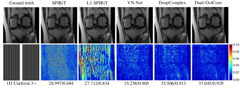
Figure 5: Comparison of different methods in terms of reconstruction accuracy, with 1D undersampling patterns and a 3$\times$ acceleration rate. Reconstruction results and error maps are presented with corresponding quantitative measurements in PSNR/SSIM.

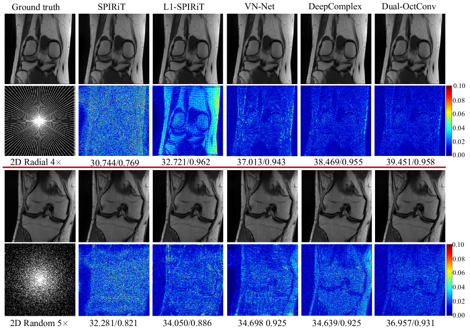
Figure 6: Comparison of different methods in terms of reconstruction accuracy, with 2D undersampling patterns and 4$\times$ and 5$\times$ acceleration rates, respectively. Reconstruction results and error maps are presented with corresponding quantitative measurements in PSNR/SSIM.

Datasets

We use the in vivo multi-coil fully-sampled MR knee dataset that is acquired using a clinical 3T Siemens Magnetom Skyra scanner with a sequence called ‘Coronal Spin Density Weighted without Fat Suppression’​ (Hammernik et al. 2018). The imaging protocol is detailed as follows: 15-channel knee coil, matrix size $320\!\times 320\!\times\!20$, TR=2750 ms, TE=27 ms, and in-plane resolution = 0.49$\times$0.44 mm². There are 20 subjects in total: 5 female/15 male, age 15-76, and BMI 20.46-32.94. We randomly select 14 patients for training, 3 for validation, and 3 for testing.

The pre-defined undersampling masks are used to obtain the undersampled measurements. In our experiments, we adopt four different $k$-space undersampling patterns, including 1D uniform, 1D Cartesian, 2D random, and 2D radial. Examples of the undersampling patterns are illustrated in Fig. 5 and Fig. 6. For 1D uniform, 1D Cartesian, and 2D random masks, the acceleration rate is set to 3 and 5. For the 2D radial mask, 4$\times$ and 6$\times$ accelerations are adopted.

Implementation Details

We implement our model using Tensorflow 1.14 and perform experiments using an NVIDIA 1080Ti GPU with a 11GB memory. Following (Wang et al. 2020), we initialize the magnitude and phase of the complex parameters using Rayleigh and uniform distributions, respectively. The network is trained using the Adam optimizer (Wang et al. 2020) with initial learning rate 0.001 and weight decay 0.95. The batch size is set to 4 and convolutional kernel size is set to $3\times 3$. Each complex convolutional layer has 64 feature maps, except for the last layer, which is determined by the concatenated real and imaginary channels of the data. The spatial frequency ratio $\alpha$ is set to $0.125$ by default.

To demonstrate its effectiveness, we compare our Dual-OctConv with a number of state-of-the-art parallel MR imaging approaches, including traditional methods (SPIRiT (Lustig and Pauly 2010) and L1-SPIRiT (Murphy et al. 2010)) as well as CNN-based methods (VN-Net (Hammernik et al. 2018) and ComplexMRI (Wang et al. 2020)). All these methods are trained on the same dataset with their default settings. For CNN-based methods, we re-trained them according to the specifications with TensorFlow, using their default parameter settings.

Quantitative Evaluation

We use peak signal-to-noise ratio (PSNR) and structural similarity index measure (SSIM) (Wang et al. 2020) for quantitative evaluation. Table 1 reports the average PSNR and SSIM results with respect to different undersampling patterns and acceleration factors. As can be seen, our Dual-OctConv obtains consistent performance improvements against the baseline methods, across various settings. Additionally, we observe that the undersampling patterns greatly affect the quality of reconstruction. For instance, the 2D sampling masks generally outperform the 1D masks. Another important observation is that the reconstruction becomes more difficult when the acceleration rate increases.

In particular, our model significantly outperforms previous methods under extremely challenging settings (i.e., 2D masks with 5$\times$ and 6$\times$ acceleration). This can be attributed to the powerful capability of our Dual-OctConv in aggregating rich contextual information of real and imaginary data. Moreover, we see that our model show strong robustness under various undersampling patterns and acceleration rates.

Qualitative Evaluation

For qualitative analysis, we first show the reconstructed images and corresponding error maps for 1D uniform with a 3$\times$ acceleration rate in Fig. 5. In general, our method provides the best-quality reconstructed images and significantly reduces prediction errors. In contrast, the baseline methods yield large prediction errors and show unsatisfactory performance. In particular, compared with the CNN-based method, the traditional methods show obvious errors, such as SPIRiT and L1-SPIRiT.

We next examine the results for 2D radial masks with a 4$\times$ acceleration rate and 2D random masks with a 5$\times$ acceleration rate. As shown in Fig. 6, CNN-based methods significantly improve the results with less errors and clearer structures, in comparison with SPIRiT and L1-SPIRiT. In particular, our Dual-OctConv produces higher-quality images with clear details and minimum artifacts. The superior performance is owed to the fact that Dual-OctConv can effectively aggregate the information of various spatial frequencies present in the real and imaginary parts of an MR image.

Ablation Studies

Firstly, we study the effects of the proposed Dual-OctConv. For comparison, we build a baseline model by setting $\alpha\!=\!0$, which turns the Dual-OctConv into a standard complex convolution. We conduct experiments on the test set with 60 complex-valued images under the uniform undersampling mask with a 3$\times$ acceleration rate. As illustrated in Fig. 7, our Dual-OctConv significantly outperforms the baseline model, especially in terms of SSIM. This reveals the superiority of the Dual-OctConv in improving the reconstruction.

Secondly, we investigate the influence of the spatial frequency ratio $\alpha$ for reconstruction. The ratio determines the receptive fields in both the real and imaginary parts, and also influences the fusion of these parts at multiple spatial frequencies. As shown in Fig. 8, our model shows the best PSNR and SSIM scores at $\alpha\!=\!0.125$, which means that 12.5% of the channels in the real and imaginary parts are reduced to a low spatial frequency. When $\alpha$ becomes larger, the performance quickly degrades due to severe information loss induced by over-large ratios.

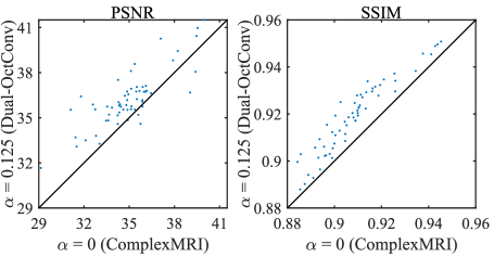
Figure 7: Quantitative comparison of Dual-OctConv and the baseline model ($\alpha\!=\!0$) in terms of PSNR and SSIM. Note that ratio $\alpha\!=\!0$ is equivalent to the complexMRI model.

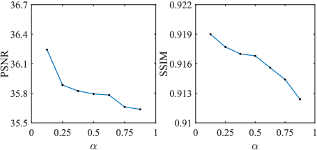
Figure 8: Analysis of spatial frequency ratio ($\alpha$) in terms of PSNR and SSIM.

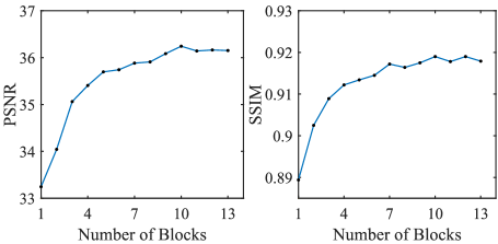
Figure 9: Performance comparison of our network with respect to the number of Dual-OctConv blocks.

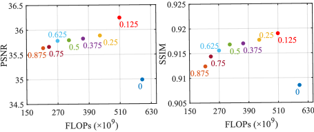
Figure 10: FLOPs analysis with respect to spatial frequency ratios ($\alpha$). The number below each point is the value of $\alpha$. We see that, under varioous settings ($0\!<\!\alpha\!<\!1$), our Dual-OctConv is always more efficient and accurate than the baseline model ($\alpha\!=\!0$).

The number of network parameters increases as the number of blocks ($bn$) increases. Therefore, it is necessary to choose an appropriate number of blocks to ensure that the network structure reaches the highest reconstruction accuracy without inducing higher computational and memory requirements. Herein, we carry out various experiments using different numbers of blocks. The results are presented in Fig. 9. As can be seen from the curves, our model can successfully reconstruct the MR images at $bn\!=\!4$, and the reconstruction accuracy reaches the highest at $bn\!=\!10$.

Finally, we study the FLOPs of Dual-OctConv with respect to different $\alpha$ in Fig. 10. The number below each point is the value of $\alpha$, and $\alpha\!=\!0$ refers to the baseline model. As can be observed, a small $\alpha$ leads to improved performance with a higher FLOPs. Moreover, compared with the baseline model (i.e., $\alpha\!=\!0$), our model consistently shows better performance with much lower FLOPs.

Conclusion

In this work, we focus on spatial frequency feature expression in complex-valued data for parallel MR image reconstruction. For this purpose, we propose a novel Dual-OctConv operation to deal with the real and imaginary components at multiple spatial frequencies. By convolving the feature maps of both the real and imaginary components under different spatial resolutions, our Dual-OctConv is able to reconstruct higher-quality images with significantly reduced artifacts. We conduct extensive experiments on an $in~{}vivo$ knee dataset under different settings of undersampling patterns and acceleration rates, and the results demonstrate the advantages of our model against state-of-the-art methods in accelerated MR image reconstruction.

References

- Aggarwal, Mani, and Jacob (2018) Aggarwal, H. K.; Mani, M. P.; and Jacob, M. 2018. MoDL: Model-based deep learning architecture for inverse problems. IEEE Transactions on Medical Imaging 38(2): 394–405.
- Chen et al. (2019a) Chen, Y.; Fan, H.; Xu, B.; Yan, Z.; Kalantidis, Y.; Rohrbach, M.; Yan, S.; and Feng, J. 2019a. Drop an octave: Reducing spatial redundancy in convolutional neural networks with octave convolution. In Proceedings of the IEEE International Conference on Computer Vision, 3435–3444.
- Chen et al. (2019b) Chen, Y.; Xiao, T.; Li, C.; Liu, Q.; and Wang, S. 2019b. Model-based convolutional de-aliasing network learning for parallel MR imaging. In International Conference on Medical Image Computing and Computer-Assisted Intervention, 30–38.
- Feng et al. (2021) Feng, C.-M.; Wang, K.; Lu, S.; Xu, Y.; and Li, X. 2021. Brain MRI Super-Resolution using Coupled-Projection Residual Network. Neurocomputing .
- Feng et al. (2019) Feng, C.-M.; Xu, Y.; Hou, M.-X.; Dai, L.-Y.; and Shang, J.-L. 2019. PCA via joint graph Laplacian and sparse constraint: Identification of differentially expressed genes and sample clustering on gene expression data. BMC bioinformatics 20(22): 1–11.
- Griswold et al. (2002) Griswold, M. A.; Jakob, P. M.; Heidemann, R. M.; Nittka, M.; Jellus, V.; Wang, J.; Kiefer, B.; and Haase, A. 2002. Generalized autocalibrating partially parallel acquisitions (GRAPPA). Magnetic Resonance in Medicine: An Official Journal of the International Society for Magnetic Resonance in Medicine 47(6): 1202–1210.
- Haldar and Zhuo (2016) Haldar, J. P.; and Zhuo, J. 2016. P-LORAKS: low-rank modeling of local k-space neighborhoods with parallel imaging data. Magnetic resonance in medicine 75(4): 1499–1514.
- Hammernik et al. (2018) Hammernik, K.; Klatzer, T.; Kobler, E.; Recht, M. P.; Sodickson, D. K.; Pock, T.; and Knoll, F. 2018. Learning a variational network for reconstruction of accelerated MRI data. Magnetic resonance in medicine 79(6): 3055–3071.
- Han et al. (2018) Han, Y.; Yoo, J.; Kim, H. H.; Shin, H. J.; Sung, K.; and Ye, J. C. 2018. Deep learning with domain adaptation for accelerated projection-reconstruction MR. Magnetic resonance in medicine 80(3): 1189–1205.
- He et al. (2016) He, J.; Liu, Q.; Christodoulou, A. G.; Ma, C.; Lam, F.; and Liang, Z.-P. 2016. Accelerated high-dimensional MR imaging with sparse sampling using low-rank tensors. IEEE Transactions on Medical Imaging 35(9): 2119–2129.
- Ke, Maire, and Yu (2017) Ke, T.-W.; Maire, M.; and Yu, S. X. 2017. Multigrid neural architectures. In Proceedings of the IEEE Conference on Computer Vision and Pattern Recognition, 6665–6673.
- Knoll et al. (2019) Knoll, F.; Hammernik, K.; Zhang, C.; Moeller, S.; Pock, T.; Sodickson, D. K.; and Akcakaya, M. 2019. Deep learning methods for parallel magnetic resonance image reconstruction. arXiv preprint arXiv:1904.01112 .
- Kwon, Kim, and Park (2017) Kwon, K.; Kim, D.; and Park, H. 2017. A parallel MR imaging method using multilayer perceptron. Medical physics 44(12): 6209–6224.
- Lee et al. (2018) Lee, D.; Yoo, J.; Tak, S.; and Ye, J. C. 2018. Deep residual learning for accelerated MRI using magnitude and phase networks. IEEE Transactions on Biomedical Engineering 65(9): 1985–1995.
- Li et al. (2018) Li, J.; Fang, F.; Mei, K.; and Zhang, G. 2018. Multi-scale residual network for image super-resolution. In Proceedings of the European Conference on Computer Vision, 517–532.
- Lin et al. (2017) Lin, T.-Y.; Dollár, P.; Girshick, R.; He, K.; Hariharan, B.; and Belongie, S. 2017. Feature pyramid networks for object detection. In Proceedings of the IEEE Conference on Computer Vision and Pattern Recognition, 2117–2125.
- Liu et al. (2019) Liu, Y.; Liu, Q.; Zhang, M.; Yang, Q.; Wang, S.; and Liang, D. 2019. IFR-Net: Iterative feature refinement network for compressed sensing mri. IEEE Transactions on Computational Imaging 6: 434–446.
- Lustig and Pauly (2010) Lustig, M.; and Pauly, J. M. 2010. SPIRiT: iterative self-consistent parallel imaging reconstruction from arbitrary k-space. Magnetic resonance in medicine 64(2): 457–471.
- Murphy et al. (2010) Murphy, M.; Keutzer, K.; Vasanawala, S.; and Lustig, M. 2010. Clinically feasible reconstruction time for L1-SPIRiT parallel imaging and compressed sensing MRI. In Proceedings of the ISMRM Scientific Meeting & Exhibition, 4854.
- Nah, Hyun Kim, and Mu Lee (2017) Nah, S.; Hyun Kim, T.; and Mu Lee, K. 2017. Deep multi-scale convolutional neural network for dynamic scene deblurring. In Proceedings of the IEEE Conference on Computer Vision and Pattern Recognition, 3883–3891.
- Nakarmi et al. (2017) Nakarmi, U.; Wang, Y.; Lyu, J.; Liang, D.; and Ying, L. 2017. A kernel-based low-rank (KLR) model for low-dimensional manifold recovery in highly accelerated dynamic MRI. IEEE Transactions on Medical Imaging 36(11): 2297–2307.
- Pruessmann et al. (1999) Pruessmann, K. P.; Weiger, M.; Scheidegger, M. B.; and Boesiger, P. 1999. SENSE: sensitivity encoding for fast MRI. Magnetic Resonance in Medicine: An Official Journal of the International Society for Magnetic Resonance in Medicine 42(5): 952–962.
- Quan, Nguyen-Duc, and Jeong (2018) Quan, T. M.; Nguyen-Duc, T.; and Jeong, W.-K. 2018. Compressed sensing MRI reconstruction using a generative adversarial network with a cyclic loss. IEEE Transactions on Medical Imaging 37(6): 1488–1497.
- Ramani and Fessler (2010) Ramani, S.; and Fessler, J. A. 2010. Parallel MR image reconstruction using augmented Lagrangian methods. IEEE Transactions on Medical Imaging 30(3): 694–706.
- Ren et al. (2016) Ren, W.; Liu, S.; Zhang, H.; Pan, J.; Cao, X.; and Yang, M.-H. 2016. Single image dehazing via multi-scale convolutional neural networks. In Proceedings of the European Conference on Computer Vision, 154–169.
- Schlemper et al. (2019a) Schlemper, J.; Duan, J.; Ouyang, C.; Qin, C.; Caballero, J.; Hajnal, J. V.; and Rueckert, D. 2019a. Data consistency networks for (calibration-less) accelerated parallel MR image reconstruction. arXiv preprint arXiv:1909.11795 .
- Schlemper et al. (2019b) Schlemper, J.; Qin, C.; Duan, J.; Summers, R. M.; and Hammernik, K. 2019b. -net: Ensembled Iterative Deep Neural Networks for Accelerated Parallel MR Image Reconstruction. arXiv preprint arXiv:1912.05480 .
- Sriram et al. (2020) Sriram, A.; Zbontar, J.; Murrell, T.; Zitnick, C. L.; Defazio, A.; and Sodickson, D. K. 2020. GrappaNet: Combining parallel imaging with deep learning for multi-coil MRI reconstruction. In Proceedings of the IEEE Conference on Computer Vision and Pattern Recognition, 14315–14322.
- Sun et al. (2019) Sun, L.; Fan, Z.; Fu, X.; Huang, Y.; Ding, X.; and Paisley, J. 2019. A deep information sharing network for multi-contrast compressed sensing MRI reconstruction. IEEE Transactions on Image Processing 28(12): 6141–6153.
- Sun et al. (2018) Sun, L.; Fan, Z.; Huang, Y.; Ding, X.; and Paisley, J. 2018. Compressed sensing MRI using a recursive dilated network. In Thirty-Second AAAI Conference on Artificial Intelligence.
- Trabelsi et al. (2018) Trabelsi, C.; Bilaniuk, O.; Serdyuk, D.; Subramanian, S.; Santos, J. F.; Mehri, S.; Rostamzadeh, N.; Bengio, Y.; and Pal, C. 2018. Deep Complex Networks. ArXiv abs/1705.09792.
- Wang et al. (2020) Wang, S.; Cheng, H.; Ying, L.; Xiao, T.; Ke, Z.; Zheng, H.; and Liang, D. 2020. DeepcomplexMRI: Exploiting deep residual network for fast parallel MR imaging with complex convolution. Magnetic Resonance Imaging 68: 136–147.
- Wang et al. (2016) Wang, S.; Su, Z.; Ying, L.; Peng, X.; Zhu, S.; Liang, F.; Feng, D.; and Liang, D. 2016. Accelerating magnetic resonance imaging via deep learning. In IEEE International Symposium on Biomedical Imaging, 514–517.
- Wang et al. (2017) Wang, S.; Tan, S.; Gao, Y.; Liu, Q.; Ying, L.; Xiao, T.; Liu, Y.; Liu, X.; Zheng, H.; and Liang, D. 2017. Learning joint-sparse codes for calibration-free parallel MR imaging. IEEE Transactions on Medical Imaging 37(1): 251–261.
- Yang et al. (2017) Yang, G.; Yu, S.; Dong, H.; Slabaugh, G.; Dragotti, P. L.; Ye, X.; Liu, F.; Arridge, S.; Keegan, J.; Guo, Y.; et al. 2017. DAGAN: Deep de-aliasing generative adversarial networks for fast compressed sensing MRI reconstruction. IEEE Transactions on Medical Imaging 37(6): 1310–1321.
- Yang et al. (2020) Yang, Y.; Sun, J.; Li, H.; and Xu, Z. 2020. ADMM-CSNet: A Deep Learning Approach for Image Compressive Sensing. IEEE Transactions on Pattern Analysis and Machine Intelligence 42(3): 521–538.
- Zhao et al. (2017) Zhao, H.; Shi, J.; Qi, X.; Wang, X.; and Jia, J. 2017. Pyramid scene parsing network. In Proceedings of the IEEE Conference on Computer Vision and Pattern Recognition, 2881–2890.
- Zhou et al. (2020a) Zhou, T.; Li, J.; Wang, S.; Tao, R.; and Shen, J. 2020a. MATNet: Motion-Attentive Transition Network for Zero-Shot Video Object Segmentation. IEEE Transactions on Image Processing 29: 8326–8338.
- Zhou et al. (2021) Zhou, T.; Qi, S.; Wang, W.; Shen, J.; and Zhu, S.-C. 2021. Cascaded Parsing of Human-Object Interaction Recognition. IEEE Transactions on Pattern Analysis and Machine Intelligence .
- Zhou et al. (2020b) Zhou, T.; Wang, S.; Zhou, Y.; Yao, Y.; Li, J.; and Shao, L. 2020b. Motion-Attentive Transition for Zero-Shot Video Object Segmentation. In Proceedings of the 34th AAAI Conference on Artificial Intelligence (AAAI), 13066–13073.