Voting-based probabilistic consensuses and their applications in distributed ledgers

Abstract

We review probabilistic models known as majority dynamics (also known as threshold voter models) and discuss their possible applications for achieving consensus in cryptocurrency systems. In particular, we show that using this approach in a straightforward way for practical consensus in a Byzantine setting can be problematic and requires extensive further research. We then discuss the Fast Probabilistic Consensus (FPC) protocol [60], which circumvents the problems mentioned above by using external randomness.

1 Introduction

The interest of academia and industry in Distributed Ledger Technology (DLT) has been steadily increasing in recent years. While DLTs are primarily known for their applications within the financial sector, they can become the key enabler for various applications in a wide variety of industries, including smart contracts, digital identity, open APIs, smart healthcare, and data marketplaces.

At the heart of each DLT lies a consensus protocol. A consensus protocol enables participants to reach a consensus about which transactions or data are accepted in the ledger. This consensus can be as simple as a binary decision as to whether a cryptocurrency transaction is valid or not. The main challenge of consensus protocols is that they have to be robust against faults and malicious participants who want to corrupt the ledger or delay the system’s consensus finding.

There are many different kinds of consensus protocols, and an “optimal” choice depends on the network situation and the actual use case; we refer to, e.g., [8]. For instance, one distinguishes between permissioned and permissionless networks, different network sizes, different grades of centrality, and different kinds of finality. In this paper, we focus on the scenario of large permissionless and decentralized networks where communication costs are essential. The obtained consensus is probabilistic in the sense that consensus is achieved with very high probability. This kind of probabilistic consensus is typical in permissionless networks since a priori not all participants are known and a deterministic finality is therefore not achievable.

The non-trivial question of how participants in a permissionless and decentralized network can reach a consensus at all was answered by the invention of Proof of Work (PoW) or Nakamoto consensus [53]. PoW or the ability (computing power) to do a cryptographic puzzle replaces a (physical) identity. In [53], Nakamoto summarizes the protocol as “(Nodes) vote with their CPU power, expressing their acceptance of valid blocks by working on extending them and rejecting invalid blocks by refusing to work on them.” Accepted blocks accumulate to chains, and participants agree on the “longest chain rule”; the distributed ledger equals the longest chain.

Unfortunately, PoW has many well-known disadvantages, such as high energy consumption and non-scalability. For this reason, many efforts have been made to either apply existing consensus protocols to DLTs or develop new ones. We again refer to [8] for an overview of the current consensus protocol landscape.

There has been a great deal of “classical” research on (probabilistic) Byzantine consensus protocols, see e.g., [2, 9, 13, 32, 34, 62]. However, the disadvantage of the approach shared by these papers is that they typically require the nodes to exchange $O(n^{2})$ messages in each round (where $n$ is the number of nodes). This can be a major barrier in situations where communication complexity matters (think about a large number of geographically spread nodes, a situation typical in cryptocurrency applications). There are cryptocurrency systems that use this approach in practice (for example, EOS, Lisk, Neo) but in order to mitigate the communication complexity issues, these effectively rely on reduced validator sets (for example, 21 nodes in EOS).

In this paper, we review the probabilistic models known as (threshold) voter models or majority dynamics. Their distinguishing feature compared with the aforementioned probabilistic Byzantine consensus protocols is their reduced communication complexity — in each round, a node only asks a constant number of other nodes for opinions. This feature makes it very tempting to use them to achieving a consensus in cryptocurrency systems — as observed above, low communication complexity can be very important in this context. We will, however, see in Section 2 that using them for consensus in a secure way is far from being easy. These models have been extensively studied in the probability and statistical physics communities since the 1970s, but are perhaps less known in the field of theoretical computer science. One of the main purposes of this paper is to introduce as rigorously as possible the (often highly non-trivial) mathematics of threshold voter models and, in particular, highlight some possible problems and challenges in their applications to consensus in Byzantine setting.

1.1 Probabilistic Voter Models: description and history

There has been extensive research on probabilistic models where, in each round, a node only contacts a small number of other nodes in order to learn their opinions, and possibly change its own. These types of models are usually referred to as voter models, and they were introduced in the 1970s by Holley and Liggett [39] and Clifford and Sudbury [18]; they are part of a larger framework of interacting particle systems [45]. Since we are talking about a broad class of models, we cannot rigorously define them all at once, but one can describe this class of models in the following way:

• There is a (finite or infinite) set of nodes that are identified with the vertices of a connected graph (usually non-oriented). An important case is that of a complete graph where every two nodes are neighbors.

• At each moment of (discrete or continuous) time, each node has an opinion (also frequently called spin in statistical physics literature) $0$ or $1$.

• At (random or deterministic) moments of time, a particular node contacts a random subset of its neighbors and asks them for their current opinions. It will then update its own opinion according to some specific rule, which depends on those queried opinions and also possibly on its own current opinion. These updates can be synchronous or asynchronous — we comment on that in Section 2.1.

• This rule has to be consistent: if a node applies the rule to an all-$0$ or all-$1$ set of opinions, then it will decide on the same opinion.

• This rule has to be monotonic: if a node decides on opinion $i\in\{0,1\}$ according to it, then it would also decide on it if we flip some of the opinions it received from $1-i$ to $i$ (i.e., when the opinion gets more support, a node cannot stop preferring it).

In practical applications, it is also frequently necessary to consider finalization rules (i.e., when a node decides that an opinion $i$ is final and will not change it anymore) that may depend on the history, not just on the last opinions received. We will comment more on that later; for now, let us only observe that it is important to understand the behavior of Markovian dynamics (i.e., when the future evolution depends only on the current state of the system, not on the past) before starting to consider additional rules of that sort.

In general, mathematicians and physicists love voter models because of their rich and interesting limiting behavior (that can e.g., give rise to hydrodynamic equations, etc.); a few notable papers are [14, 23, 24, 61, 69]. In the present paper, however, we will concentrate on their consensus applications. A very important observation is that, in most cases, voter models have only two extremal invariant measures: one concentrated on the all-$0$ configuration, and the other on all-$1$ configuration — we can naturally call these two configurations “consensus states”. This fact makes voter models interesting for decentralized consensus applications.

In this class of models, one can distinguish between different kinds of network topologies. A first observation is that the better the connectivity of this network, the faster the process converges to one of the extremal measures, see e.g., [1, 10, 36].

The next observation that can be made is that the convergence property depends on the distribution of the initial opinions. In cases where the initial densities are chosen at random and the density of $1$s is significantly different from $\tfrac{1}{2}$, recent research shows that consensus can quickly be found with a very high probability, see e.g., [21, 22, 25, 29, 31, 50]. More precisely, the overall communication complexity is $O(n\ln n)$; hence, every node has to issue only $O(\ln n)$ queries. These results clearly serve as a motivation for the further study of possible applications of voting-based protocols for consensus in real-world systems.

However, convergence can fail for some fixed initial configurations. Moreover, for instance [72] contains results that show the fragility of the protocol on initial configurations. There are only a few results in the presence of an adversary. For instance, in [7, 27] robustness was proven for particular cases for an adversary controlling up to $o(\sqrt{n})$ nodes.

Besides the more theoretical works cited above, there have been various more applied works to understand voting protocols. Again, it was shown that these voting protocols may achieve good performances in noiseless and undisturbed networks. However, their performance significantly decreases with noise [35, 37, 41] or errors [49] and may completely fail in a Byzantine setting [15]. This weak robustness in the face of faulty nodes may explain why simple majority voting has not been thoroughly investigated (in the context of practical applications) until recently. Let us also cite [40, 63] for a statistical-physics approach to applications of the voter model in social sciences and refer to [55] for an analysis of opinions dynamics with the help of potentials. These works also confirm that the road to consensus might not be straightforward: as stated in [63], “A basic message from these modeling efforts is that incorporating any realistic feature of decision making typically leads to either a dramatically hindered approach to consensus or to the prevention of consensus altogether.”

We also have to mention another related class of models: cellular automata [19, 74]. Many kinds of cellular automata (especially when used in consensus applications, e.g., [1, 10, 36, 71]) work in a way similar to the models discussed earlier in this section: each node asks its neighbors for opinions and then updates its own opinion using some kind of deterministic rule (e.g., a majority one). The dynamics are also usually synchronous (all nodes update their status at the same moment), which makes the evolution of the process completely deterministic (although there may be some randomness in the choice of initial configuration and/or in the choice of the underlying connection graph). This determinism makes the mathematical treatment of these models quite different (and usually also quite harder!) from what will be seen in this paper; for this reason, we have chosen to exclude this (very interesting) class of models from the present analysis and concentrate on models with probabilistic dynamics. Still, we should mention that usage of a deterministic majority dynamics cellular automata was recently proposed in the NKN cryptocurrency system [54]. On the other hand, in [64, 65] a probabilistic voting-based consensus protocol, similar to the models discussed in this paper, was proposed to be used in the Avalanche cryptocurrency system. However, the authors of [64] and [65] fail to properly analyze their proposed protocol and the question of whether it has the desired properties remains unclear. We refer to the end of Section 2.3 for a more detailed discussion.

1.2 Outline

In the following lines, we describe the contents of this paper. In Section 2 we use an example of asynchronous majority dynamics to explain the methods used for analysing it in the simplest setting (Section 2.1) and then in the presence of Byzantine actors (Section 2.2). To this end, we introduce and explain the concept of “random walk on a potential landscape”, which gives an excellent heuristic to understand why, once there is a considerable majority, the protocol quickly converges, but also that there is an intrinsic problem that hinders good performance in Byzantine infrastructures.

In Section 2.3 we discuss the challenges and difficulties that, due to the metastability phenomenon, arise when one intends to justify the usage of the majority dynamics models for practical consensus in a Byzantine setting. In particular, Byzantine actors can cause metastable states; metastability obliterates liveness and can compromise safety too.

Then, in Section 3 we discuss the Fast Probabilistic Consensus (FPC) protocol: we introduce the necessary notation and define it in Section 3.1, we discuss a few possible adversarial strategies in Section 3.2, some relevant theoretical results are stated in Section 3.3, and Section 3.4 is devoted to discussions of simulation results and generalizations.

2 Majority dynamics in the presence of Byzantine actors

At this point, we would like to mention that studying these sort of models requires advanced probabilistic tools and their rigorous treatment is in many aspects beyond the scope of this paper. Therefore, in this section, we will do our best to intuitively explain the relevant ideas. To this end, we consider a toy model that allows discussing the nature of majority dynamics without getting lost in technicalities.

Another important remark is that, when one is studying the possible applications of these models to consensus in DLT, it is essential to be able to obtain quantitative estimates for probabilities of relevant events, and this complicates matters even more. Elaborating on the last point, it is not infrequent to find in the literature roughly the following definitions of the safety of the system: “for any $\varepsilon>0$ it is possible to adjust parameters in such a way that the probability that some two nodes would decide differently on the validity of a particular transaction does not exceed $\varepsilon$”. This, however, is hardly acceptable, at least in the case when one wants to show that the system scales up well (with respect to the total number of nodes), for the following reason. Typically, the participants in the system want to participate in it, which means not only validating transactions but also issuing them. Then, if those $n$ nodes work during time $T$, there would typically be $O(nT)$ transactions and all of them need to be secure. Hence, for example, a safety estimate with $\varepsilon=\frac{1}{\sqrt{n}}$ will not be of much help (as one will not be able to use the union bound for estimating the probability of at least one “safety violation”). Also, when discussing the liveness guarantees (i.e., that the consensus on the state of a transaction eventually occurs), being able to obtain explicit estimates is also very important.

To underline the relevance of the last point, a somewhat extreme example is the statement “Bitcoin addresses are insecure” with the following “proof”: indeed, the space of all possible private keys is finite, therefore an adversary who just tries them subsequently would eventually find the right one. However, since nearly every $256$-bit number is a valid ECDSA private key, the probability of guessing a given private key is of the order $10^{-77}$. Hence, one would need roughly $10^{77}$ tries to find the right one; with the current state of technology, this essentially means “never”. Therefore, whenever possible, we will aim for explicit estimates (at least those with a clear asymptotic behavior with respect to the system’s size).

2.1 A simple majority dynamics model and its properties

Probably the most accessible way to understand majority dynamics models is by visualizing them as a random motion on a potential landscape. To explain this, we will consider a toy model, which is a variant of a discrete-time asynchronous majority dynamics on a complete graph. Generally, mathematicians love playing with toy models: they are easier to treat, but already contain the main ideas necessary to understand more complicated models. Usually, toy models give us insight into phenomena to expect in more complicated models of the same kind. We will also use this model to present some probabilistic tools and show how they are usually used in the analysis of models of this class. Our toy model is defined in the following way. The system consists of $n$ nodes, and at each (discrete) time moment one of them is selected uniformly at random. The selected node then chooses three nodes independently and uniformly at random. In particular, it may choose itself, and also may choose some nodes more than once; in the last case the corresponding opinions are counted the same number of times. The selected node then adopts the majority opinion of the chosen nodes until it is selected again. In this subsection there will be no Byzantine nodes; that is, for now we are assuming that all nodes follow the protocol honestly.

Before proceeding, let us also comment on our choice of model. We have chosen it to be asynchronous. More precisely, it is an embedded discrete-time process of an asynchronous continuous-time model where, at each time moment, at most $1$ node updates its preference. Another natural choice would be a round-based or synchronous model: at a given round, all nodes choose their random peers independently and update their preferences based on the responses. For this kind of dynamic, one can likely use the same intuition, but the rigorous treatment of the synchronous model becomes more difficult because it can no longer be represented by a nearest-neighbor random walk; analyzing a non-nearest-neighbor random walk in a rigorous way may be a much more challenging task.

In the following, let us additionally assume that $n\geq 20$ and that $n$ is divisible by $4$ — this will spare us from having to deal with integer parts at some places, and it is a toy model anyway.

We denote by $X_{k}$ the number of nodes with opinion $1$ at time $k$. Assume $X_{k}=m$; the number of $1$-opinions among three independently-chosen (with possible repetitions) nodes then has the Binomial$\big{(}3,\frac{m}{n}\big{)}$ distribution. Then, if one of the $m$ opinion-$1$ nodes was selected (which happens with probability $\frac{m}{n}$), it will switch its opinion to $0$ with probability $\big{(}1-\frac{m}{n}\big{)}^{3}+3\big{(}1-\frac{m}{n}\big{)}^{2}\frac{m}{n}$; likewise, if a node with current opinion $0$ was selected (which happens with probability $1-\frac{m}{n}$), it will switch its opinion to $1$ with probability $\big{(}\frac{m}{n}\big{)}^{3}+3\big{(}1-\frac{m}{n}\big{)}\big{(}\frac{m}{n}\big{)}^{2}$. In particular, and as expected, $0$ and $n$ are absorbing states: if $X_{k_{0}}\in\{0,n\}$ for some $k_{0}$ then $X_{k}=X_{k_{0}}$ for all $k>k_{0}$. In other words, the process $(X_{k},k\geq 0)$ is a (one-dimensional) random walk on $\{0,\ldots,n\}$ with the following transition probabilities: on $X_{k}=m\in\{0,\ldots,n-1\}$ we have

$$X_{k+1}=\begin{cases}m-1,&\text{with probability }p_{m},\\ m+1,&\text{with probability }q_{m},\\ m,&\text{with probability }v_{m}=1-p_{m}-q_{m},\end{cases}$$ (1)

where

$$p_{m} =\tfrac{m}{n}\big{(}\big{(}1-\tfrac{m}{n}\big{)}^{3}+3\big{(}1-\tfrac{m}{n}\big{)}^{2}\tfrac{m}{n}\big{)}=\tfrac{m}{n}\big{(}1-\tfrac{m}{n}\big{)}\big{(}\big{(}1-\tfrac{m}{n}\big{)}^{2}+3\tfrac{m}{n}\big{(}1-\tfrac{m}{n}\big{)}\big{)},$$

$$q_{m} =\big{(}1-\tfrac{m}{n}\big{)}\big{(}\big{(}\tfrac{m}{n}\big{)}^{3}+3\big{(}1-\tfrac{m}{n}\big{)}\big{(}\tfrac{m}{n}\big{)}^{2}\big{)}=\tfrac{m}{n}\big{(}1-\tfrac{m}{n}\big{)}\big{(}\big{(}\tfrac{m}{n}\big{)}^{2}+3\tfrac{m}{n}\big{(}1-\tfrac{m}{n}\big{)}\big{)},$$

$$v_{m} =1-\tfrac{m}{n}\big{(}1-\tfrac{m}{n}\big{)}\big{(}1+4\tfrac{m}{n}\big{(}1-\tfrac{m}{n}\big{)}\big{)}.$$

Before going into further details, let us discuss the following important intuitive idea. Sometimes it is convenient to think about a one-dimensional random walk as a random motion of a “Brownian particle” over a mountainous landscape. The particle moves randomly, but it prefers to move downhill; hopefully, Figure 1 speaks for itself.

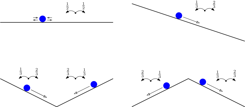
Figure 1: Intuition: random motion on top of a potential; the corresponding transition probabilities are indicated above each of the four pictures.

For example, in the top left picture, the particle has no drift and therefore just moves around in a diffusive way. In the top right picture, the particle prefers to go to the right (i.e., it has a drift in that direction), on the bottom left picture it would be “attracted” by the center of the “valley” (or potential well, as we will mostly call it in the sequel) and will probably stay there for a long time (we will elaborate on that later in this paper), while in the bottom right picture the particle (if starting at the center) would randomly choose one of the slopes and then go downhill.

Now let us go back to the random walk defined in (1). Note that the above transition probabilities are symmetric, in the sense that $p_{n-m}=q_{m}$ and $q_{n-m}=p_{m}$, which implies that

$$\frac{p_{n-m}}{q_{n-m}}=\frac{q_{m}}{p_{m}}.$$ (2)

Let us define the function $V:\{0,\ldots,n-1\}\mapsto{\mathbb{R}}$ (frequently called the potential) by $V(0)=0$ and

$$V(k)=\sum_{j=1}^{k}\log\frac{p_{j}}{q_{j}}.$$ (3)

Then, (2) implies that $V(n-1)=0$ and, in general, $V(m)=V(n-1-m)$ (that is, it is symmetric around $\frac{n-1}{2}$); in particular, $V(\tfrac{n}{2}-1)=V(\tfrac{n}{2})$. Moreover, since $p_{m}>q_{m}$ for $m<n/2$, we see that $V(m)>0$ for $0<m<n$, it is strictly increasing on $[0,\tfrac{n}{2}-1]$ and strictly decreasing on $[\tfrac{n}{2},n-1]$. This potential will be the “landscape profile” that the walker walks on, and it in fact resembles the bottom right profile on Figure 1. With some more analysis, it is not difficult to obtain that it closely resembles the profile on Figure 2.

Figure 2: The potential $V$.

Indeed, we have

$$\frac{p_{m}}{q_{m}}=f(\tfrac{m}{n}),\qquad\text{where }f(u)=\frac{(1-u)^{2}+3u(1-u)}{u^{2}+3u(1-u)},$$ (4)

and it is elementary to see that $f$ is a strictly decreasing function on the interval $(0,1)$ with $f(\tfrac{1}{2})=1$ (and also $f(1-u)=1/f(u)$). Note also that $\log\frac{p_{m}}{q_{m}}\approx 0$ when $m$ is close to $\tfrac{n}{2}$.

One of the interesting features of the potential defined above is that it can be used for computing the escape probabilities from an interval. Let $\tau_{A}=\min\{n\geq 1:X_{n}\in A\}$ denote the hitting time of a set $A$, and we abbreviate $\tau_{a}:=\tau_{\{a\}}$ for singletons. We will also use the notations ${\mathbb{P}}_{x}$ and ${\mathbb{E}}_{x}$ for the probability and expectations with respect to the process started at $x$. The next result (see e.g., Lemma 1 of [68]) is a useful tool for estimating exit probabilities from intervals.

Lemma 2.1.

For $0\leq a<x<b\leq n$ it holds that

$${\mathbb{P}}_{x}[\tau_{b}<\tau_{a}]=\frac{\sum_{y=a}^{x-1}e^{V(y)}}{\sum_{y=a}^{b-1}e^{V(y)}}.$$ (5)

Proof.

Define

$$g(m)=1+\frac{p_{1}}{q_{1}}+\cdots+\frac{p_{1}\ldots p_{m-1}}{q_{1}\ldots q_{m-1}}=\sum_{j=0}^{m-1}e^{V(j)}.$$

A straightforward computation shows that $p_{m}g(m-1)+q_{m}g(m+1)+v_{m}g(m)=g(m)$ for $1\leq m\leq n-1$, which implies that the process $g(X_{j\wedge\tau_{\{0,n\}}})$ is a martingale. The Optional Stopping Theorem (see e.g., Section 5.7 of [28]) then gives that

$$g(x)={\mathbb{P}}_{x}[\tau_{b}<\tau_{a}]g(b)+\big{(}1-{\mathbb{P}}_{x}[\tau_{b}<\tau_{a}]\big{)}g(a);$$

solving the above for ${\mathbb{P}}_{x}[\tau_{b}<\tau_{a}]$ we obtain (5). ∎

Let us note that, when dealing with expressions like (5), it is frequently possible to use the heuristic reasoning “the sum of exponentials is usually roughly of order of its maximal term”. In general, (5) justifies the intuition that the random walker “prefers to go downhill” — indeed, due to the previous observation, the probability of going “over a potential wall” (or “climbing to the top of the hill”) should typically be very small. We also note that, for a fine study of one-dimensional random walks on a potential, one can use relevant spectral tools similarly to, e.g., [20]. As an immediate consequence of Lemma 2.1 we obtain the following fact about probabilities to reach consensus on the initially preferred value in an already biased situation.

Corollary 2.2.

Assume that $0\leq x<\tfrac{n}{2}$. Then

$${\mathbb{P}}_{x}\big{[}\tau_{0}<\tau_{n}\big{]}={\mathbb{P}}_{n-x}\big{[}\tau_{n}<\tau_{0}\big{]}\geq 1-x\exp\big{(}-\big{(}V\big{(}\tfrac{n}{2}\big{)}-V(x)\big{)}\big{)}.$$ (6)

In particular, if $\tfrac{x}{n}\leq\alpha<\tfrac{1}{2}$, it holds that

$${\mathbb{P}}_{x}\big{[}\tau_{0}<\tau_{n}\big{]}\geq 1-\tfrac{n}{2}e^{-c_{\alpha}n},$$ (7)

where $c_{\alpha}>0$ depends on $\alpha$ but not on $n$.

Proof.

Note that since ${\mathbb{P}}_{x}[\tau_{0}<\tau_{n}]\geq{\mathbb{P}}_{x}[\tau_{0}<\tau_{{n}/{2}}]$ for $0<x<\tfrac{n}{2}$, we will bound the latter probability. Then, (6) easily follows from the monotonicity of $V$ on $\big{[}0,\tfrac{n}{2}\big{]}$ (bound the numerator of (5) from above by the maximal term times the number of terms, and bound the denominator of (5) from below by the maximal term). To obtain (7), we abbreviate $y=\big{\lfloor}\big{(}\tfrac{1}{4}+\tfrac{\alpha}{2}\big{)}n\big{\rfloor}$ and write

$$V\big{(}\tfrac{n}{2}\big{)}-V(x)\geq\sum_{j=x+1}^{y}\log\frac{p_{j}}{q_{j}}\geq\big{(}\big{(}\tfrac{1}{4}-\tfrac{\alpha}{2}\big{)}n-1\big{)}\log\frac{p_{y}}{q_{y}},$$

and then use (4) and (6). ∎

As mentioned before, the preceding result implies that the “significantly leading” opinion (i.e., an opinion which is shared by at least a proportion $\alpha>\tfrac{1}{2}$) does not in the end prevail only with an exponentially small (in $n$) probability.

Next, we estimate the expected time until one of the two “consensus states” is reached:

Lemma 2.3.

For any $x\in\{1,\ldots,n-1\}$ it holds that ${\mathbb{E}}_{x}\tau_{\{0,n\}}\leq\tfrac{256}{15}n(1+\log n)$.

Proof.

First, denote

$$Y_{t}=\begin{cases}X_{t},&\text{if }X_{t}\leq\tfrac{n}{2},\\ n-X_{t},&\text{if }X_{t}>\tfrac{n}{2};\end{cases}$$

by symmetry, the process $Y$ is a Markov chain with state space $\big{\{}0,\ldots,\tfrac{n}{2}\big{\}}$, and it has the same transition probabilities as $X$ on $\{0,\ldots,\tfrac{n}{2}-1\}$. Also, it is clear that it is enough to consider the worst-case $x=\tfrac{n}{2}$.

For the process $Y$, denote by $T_{m}$ the expected hitting time of $0$ starting from $m$. It is straightforward to obtain for $0<m<\tfrac{n}{2}$ that

$$T_{m}=1+p_{m}T_{m-1}+v_{m}T_{m}+q_{m}T_{m+1},$$ (8)

and

$$T_{\tfrac{n}{2}}=\tfrac{1}{2}T_{\tfrac{n}{2}}+\tfrac{1}{2}T_{\tfrac{n}{2}-1}+1,$$ (9)

since $v_{\tfrac{n}{2}}=\tfrac{1}{2}$.

Remark 2.4.

Note that (8) and (9) imply that

$$T_{m}-T_{m-1}=\frac{1}{p_{m}}+\frac{q_{m}}{p_{m}}(T_{m+1}-T_{m})$$

and

$$T_{\tfrac{n}{2}}-T_{\tfrac{n}{2}-1}=2.$$

Using this, the above system of equations can be solved to obtain

$$T_{m}=\sum_{j=1}^{m}\Bigg{(}2\prod_{\ell=j}^{\tfrac{n}{2}-1}\frac{q_{\ell}}{p_{\ell}}+\frac{1}{p_{j}}\sum_{k=j}^{\tfrac{n}{2}-2}\prod_{\ell=j}^{k}\frac{q_{\ell}}{p_{\ell+1}}\Bigg{)}.$$ (10)

However, the problem with expressions such as (10) is that it is not easy to deduce the asymptotic behavior of $T_{\tfrac{n}{2}}$ for the $p$’s and $q$’s defined below Equation (1).

To prove Lemma 2.3, we will therefore take another route, namely the Lyapunov’s functions method. This method will permit us to estimate $T_{\tfrac{n}{2}}$ without too heavy calculations. Also, it is worth noting that this method is more robust, in the sense that it may still work in the non-nearest-neighbor case when the exact expressions such as (10) are not available.

To explain the idea of this method, consider a function $f:\big{\{}0,\ldots,\tfrac{n}{2}\big{\}}\mapsto{\mathbb{R}}_{+}$ defined by $f(0)=0$ and $f(m)=T_{m}$ for $m\in\big{\{}1,\ldots,\tfrac{n}{2}\big{\}}$. Then, observe that (8) and (9) imply

$${\mathbb{E}}_{m}\big{(}f(Y_{1})-f(m)\big{)}=-1$$ (11)

for all $m\in\big{\{}1,\ldots,\tfrac{n}{2}\big{\}}$. Now, instead of trying to calculate $f$, the idea is to find a Lyapunov function $g:\big{\{}0,\ldots,\tfrac{n}{2}\big{\}}\mapsto{\mathbb{R}}_{+}$ which behaves similarly to $f$ in the sense that, for some $\varepsilon>0$

$${\mathbb{E}}_{m}\big{(}g(Y_{1})-g(m)\big{)}\leq-\varepsilon;$$ (12)

Theorem 2.6.2 of [48] then implies that ${\mathbb{E}}_{m}\tau_{0}\leq\varepsilon^{-1}g(m)$ for all $m>0$.

Let $\delta_{n}:=\lceil\sqrt{n}\,\rceil-\tfrac{n}{\lceil\sqrt{n}\,\rceil}\in[0,1)$ (observe also that $\tfrac{n}{2}-\lceil\sqrt{n}\,\rceil\geq\tfrac{n}{4}$ for $n\geq 20$), and define for $1\leq m\leq\frac{n}{2}$

$$\Delta_{m}=\begin{cases}\frac{n}{m}+2,&\text{ for }m<\frac{n}{4},\\ \frac{n}{\tfrac{n}{2}-m}+2,&\text{ for }\frac{n}{4}\leq m<\tfrac{n}{2}-\lceil\sqrt{n}\,\rceil,\\ \frac{n}{2}-m+2-\delta_{n},&\text{ for }\tfrac{n}{2}-\lceil\sqrt{n}\,\rceil\leq m\leq\tfrac{n}{2}.\end{cases}$$

Note that there is continuity in the sense that the first formula is also valid for $m=\tfrac{n}{4}$ and the second formula is also valid for $m=\tfrac{n}{2}-\lceil\sqrt{n}\,\rceil$. Let us define $g(m)=\Delta_{1}+\cdots+\Delta_{m}$. Then, observe that (recall that $v_{\tfrac{n}{2}}=\tfrac{1}{2}$)

$${\mathbb{E}}_{\tfrac{n}{2}}\big{(}g(Y_{1})-g(\tfrac{n}{2})\big{)}=-\tfrac{1}{2}\Delta_{\tfrac{n}{2}}\leq-\tfrac{1}{2},$$ (13)

and, for $m<\tfrac{n}{2}$

$${\mathbb{E}}_{m}\big{(}g(Y_{1})-g(m)\big{)} =p_{m}g(m-1)+v_{m}g(m)+q_{m}g(m+1)-g(m)$$

$$=p_{m}(g(m-1)-g(m))+q_{m}(g(m+1)-g(m))$$

$$=-p_{m}\Delta_{m}+q_{m}\Delta_{m+1}.$$ (14)

Note also that, since $p_{m}\geq q_{m}$, for the sake of upper bounds we can always drop the “$+2$” (as well as “$+2-\delta_{n}$”) part from the calculations. For $m<\tfrac{n}{4}$ (equivalently, $\tfrac{m}{n}<\tfrac{1}{4}$), we have

$$-p_{m}\Delta_{m}+q_{m}\Delta_{m+1} \leq-\tfrac{m}{n}\big{(}1-\tfrac{m}{n}\big{)}\Big{(}\tfrac{n}{m}\big{(}\big{(}1-\tfrac{m}{n}\big{)}^{2}+3\tfrac{m}{n}\big{(}1-\tfrac{m}{n}\big{)}\big{)}$$

$$\qquad\qquad\qquad\qquad-\tfrac{n}{m+1}\big{(}\big{(}\tfrac{m}{n}\big{)}^{2}+3\tfrac{m}{n}\big{(}1-\tfrac{m}{n}\big{)}\big{)}\Big{)}$$

$$\leq-\big{(}1-\tfrac{m}{n}\big{)}\Big{(}\big{(}1-\tfrac{m}{n}\big{)}^{2}-\big{(}\tfrac{m}{n}\big{)}^{2}\Big{)}$$

$$=-\big{(}1-\tfrac{m}{n}\big{)}\big{(}1-2\tfrac{m}{n}\big{)}$$

$$\leq-\tfrac{3}{8}.$$

Then, for $\frac{n}{4}\leq m<\tfrac{n}{2}-\lceil\sqrt{n}\,\rceil$ we can write

$$-p_{m}\Delta_{m}+q_{m}\Delta_{m+1}$$***

$$\leq-\tfrac{m}{n}\big{(}1-\tfrac{m}{n}\big{)}\Big{(}\tfrac{n}{\tfrac{n}{2}-m}\big{(}\big{(}1-\tfrac{m}{n}\big{)}^{2}+3\tfrac{m}{n}\big{(}1-\tfrac{m}{n}\big{)}\big{)}$$

$$\qquad\qquad\qquad\qquad-\tfrac{n}{\tfrac{n}{2}-m-1}\big{(}\big{(}\tfrac{m}{n}\big{)}^{2}+3\tfrac{m}{n}\big{(}1-\tfrac{m}{n}\big{)}\big{)}\Big{)}$$

$$=-\tfrac{m}{n}\big{(}1-\tfrac{m}{n}\big{)}\Big{(}\tfrac{n}{\tfrac{n}{2}-m}\big{(}1-\tfrac{m}{n}\big{)}^{2}-\tfrac{n}{\tfrac{n}{2}-m}\big{(}\tfrac{m}{n}\big{)}^{2}+\tfrac{n}{\tfrac{n}{2}-m}\big{(}\tfrac{m}{n}\big{)}^{2}$$

$$\qquad-\tfrac{n}{\tfrac{n}{2}-m-1}\big{(}\tfrac{m}{n}\big{)}^{2}-3\tfrac{m}{n}\big{(}1-\tfrac{m}{n}\big{)}\frac{n}{(\tfrac{n}{2}-m)(\tfrac{n}{2}-m-1)}\Big{)}$$

$$=-\tfrac{m}{n}\big{(}1-\tfrac{m}{n}\big{)}\Big{(}2-\big{(}\big{(}\tfrac{m}{n}\big{)}^{2}+3\tfrac{m}{n}\big{(}1-\tfrac{m}{n}\big{)}\big{)}\frac{n}{(\tfrac{n}{2}-m)(\tfrac{n}{2}-m-1)}\Big{)}$$

 (note that $$h(1-h)\in[\tfrac{3}{16},\tfrac{1}{4}] h\in[\tfrac{1}{4},\tfrac{1}{2}] \leq 1$$ for and that the last fraction is )

$$\leq-\tfrac{3}{16}.$$

Finally, for $\tfrac{n}{2}-\lceil\sqrt{n}\,\rceil\leq m<\tfrac{n}{2}$ we have

$$-p_{m}\Delta_{m}+q_{m}\Delta_{m+1} \leq-\tfrac{m}{n}\big{(}1-\tfrac{m}{n}\big{)}\Big{(}\big{(}\tfrac{n}{2}-m\big{)}\big{(}\big{(}1-\tfrac{m}{n}\big{)}^{2}+3\tfrac{m}{n}\big{(}1-\tfrac{m}{n}\big{)}\big{)}$$

$$\qquad\qquad\qquad\qquad-\big{(}\tfrac{n}{2}-m-1\big{)}\big{(}\big{(}\tfrac{m}{n}\big{)}^{2}+3\tfrac{m}{n}\big{(}1-\tfrac{m}{n}\big{)}\big{)}\Big{)}$$

$$=-\tfrac{m}{n}\big{(}1-\tfrac{m}{n}\big{)}\Big{(}\big{(}\tfrac{n}{2}-m\big{)}\big{(}1-2\tfrac{m}{n}\big{)}+\big{(}\tfrac{m}{n}\big{)}^{2}+3\tfrac{m}{n}\big{(}1-\tfrac{m}{n}\big{)}\Big{)}$$

(again use that $$h(1-h)\in[\tfrac{3}{16},\tfrac{1}{4}] h\in[\tfrac{1}{4},\tfrac{1}{2}]$$ for and that the first term in the parentheses is nonnegative)

$$\leq-\tfrac{15}{128}.$$

Gathering the pieces, we find that (12) holds with $\varepsilon=\tfrac{15}{128}$. It is also not difficult to obtain that

$$g\big{(}\tfrac{n}{2}\big{)} =\Delta_{1}+\cdots+\Delta_{\tfrac{n}{2}}$$

$$\leq n+\sum_{m=1}^{\tfrac{n}{4}-1}\frac{n}{m}+\sum_{m=\tfrac{n}{4}}^{\tfrac{n}{2}-\lceil\sqrt{n}\,\rceil-1}\frac{n}{\tfrac{n}{2}-m}+\sum_{m=\tfrac{n}{2}-\lceil\sqrt{n}\,\rceil}^{\tfrac{n}{2}}\big{(}\tfrac{n}{2}-m\big{)}$$

$$\leq 2n(1+\log n).$$

Then, using Theorem 2.6.2 of [48] we conclude the proof of Lemma 2.3. ∎

The constant $\tfrac{256}{15}$ in Lemma 2.3 can be improved, but we need not concern ourselves with that here. One due observation, however, is that this result gives the correct order of the expectation of the hitting time (at least for the case $\log x\asymp\log n$); this can be easily seen from the fact that $p_{m}+q_{m}\asymp\tfrac{m}{n}$ as $m$ decreases to $0$.

Corollary 2.5.

For any $x$ and any positive integer $k$ it holds that

$${\mathbb{P}}_{x}\Big{[}\tau_{\{0,n\}}>k\big{\lceil}\tfrac{512}{15}n(1+\log n)\big{\rceil}\Big{]}\leq 2^{-k}.$$ (15)

Proof.

Indeed, Chebyshev’s inequality together with Lemma 2.3 imply that

$${\mathbb{P}}_{x}\big{[}\tau_{\{0,n\}}>\tfrac{512}{15}n(1+\log n)\big{]}\leq\tfrac{1}{2}.$$

A straightforward coin-tossing argument (think about dividing the time interval $\big{[}0,k\big{\lceil}\tfrac{512}{15}n(1+\log n)\big{\rceil}\big{]}$ into $k$ subintervals of length $\big{\lceil}\tfrac{512}{15}n(1+\log n)\big{\rceil}$ and note that on each subinterval $\tau_{\{0,n\}}$ occurs with probability at least $\tfrac{1}{2}$) then implies (15). ∎

Now, let us summarize what we have obtained for our majority dynamics toy model. We have seen that:

• Lemma 2.3 and Corollary 2.5 imply that the system converges rather quickly on one of the two consensus states. Note also that, since a particular node is only selected roughly once every $n$ rounds, it will, on average, only update its state a logarithmic number of times.

• Corollary 2.2 shows that, if the overall opinions are already biased to one of the sides, then with high probability the system will achieve consensus on that prevailing opinion.

Also, thanks to the quantitative estimates that we have obtained, one can prove that the system can scale well: if it has to come to consensus on $O(n^{\gamma})$ number of bits for some fixed $\gamma>1$, we will still be able to prove that it can do this with high probability simply by using the union bounds. Having in mind practical applications, one can also analyze local finalization rules for the nodes, for example of the following type: “if last $N$ instances of my queries have all returned the same result, then consider this opinion to be final” (as previously mentioned, these local rules may be needed because in practice there might be no central authority who is able to tell that the system finds itself in one of the two consensus states).

Due to the above considerations, one may be tempted to think that a system based on a majority dynamics consensus can be used for practical applications that demand low communication complexity. This may indeed be the case in situations when all nodes are honest. However, in the next section, we will see that the presence of Byzantine nodes can significantly complicate the situation — it will no longer be possible to analyze the system in such a simple-and-elementary way as in Section 2.1.

2.2 Enter Byzantine nodes

Before discussing those, we need to develop a better understanding of (nearest-neighbor) random walks on top of a potential profile. Let us consider a one-dimensional random walk ${\widehat{X}}$ on the state space $[a,b]\subset{\mathbb{Z}}$; analogously to (1), we denote ${\hat{p}}_{x}:={\mathbb{P}}_{x}[{\widehat{X}}_{1}=x-1]$, ${\hat{q}}_{x}:={\mathbb{P}}_{x}[{\widehat{X}}_{1}=x+1]$, ${\hat{v}}_{x}:={\mathbb{P}}_{x}[{\widehat{X}}_{1}=x]$, ${\hat{p}}_{x}+{\hat{q}}_{x}+{\hat{v}}_{x}=1$ for all $x\in[a,b]$ (and, naturally, ${\hat{p}}_{a}={\hat{q}}_{b}=0$). Then, define the potential ${\widehat{V}}$ analogously to (3), with ${\hat{p}}$’s and ${\hat{q}}$’s on the place of $p$’s and $q$’s.

Now, the question is: suppose that we know what the potential ${\widehat{V}}$ looks like; for example, it could be as shown in Figure 3.

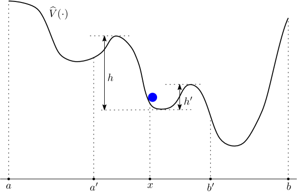
Figure 3: Random walk on a potential.

Based on this, what can we say about the properties of the process ${\widehat{X}}$?

In the following few lines, we will formulate some principles that would permit us to understand the behavior of the random walk as a function of the potential, at least on an intuitive level. This intuition can be turned into rigorous arguments; the exact formulations (let alone proofs) are beyond the scope of this paper; but let us cite the seminal paper [68] where this sort of analysis was applied to random walks in random environments to characterize its highly non-trivial behavior in the recurrent regime. We will also assume that the random walk does not have any absorbing states (in contrast to the one in the previous section) – we will see that this will be the case in the presence of Byzantine nodes anyway. Let us also keep in mind that the following intuition typically applies to various reasonable definitions of the potential and that we are trying to understand processes with large state spaces. For this reason we will not try to be excessively precise when making pictures, e.g., we represent the potential by continuous graphs even though it is defined on a discrete domain, and, for example, we pretend that $an$ and $an+1$ are indistinguishable on the picture when $n$ is large.

Claim 2.6.

The random walk on top of a potential roughly behaves in the following way:

• it “prefers” to go downhill;

• the probability that it goes in an “improbable direction” is roughly the exponential of minus the difference of “heights to overcome” (for example, on Figure 3, ${\mathbb{P}}_{x}[\tau_{a^{\prime}}<\tau_{b^{\prime}}]\approx e^{-(h-h^{\prime})}$);

• its stationary distribution at $x$ is roughly proportional to $e^{-{\widehat{V}}(x)}$; so, in the long run, the process will stay for the overwhelming amount of time at the bottom(s) (global minima) of the potential;

• The time to go out of a potential well of depth $h^{\prime}$ (such as the one where the walker currently is on Figure 3) is roughly an Exponential random variable with the expected value $\approx e^{h^{\prime}}$.

We justify the above in the following way. Item (i) is clear from the definition, and (ii) is essentially a consequence of Lemma 2.1 (together with the observation about sums of exponentials after it). As for (iii), from the fact that the Markov chain is reversible, we obtain that the stationary distribution at $x$ is exactly proportional to $\frac{{\hat{q}}_{a}\cdots{\hat{q}}_{x-1}}{{\hat{p}}_{a+1}\cdots{\hat{p}}_{x}}$; now, this is in fact almost $e^{-{\widehat{V}}(x)}$. Regarding (iv), note that it is quite common for the hitting times of Markov chains to have approximately Exponential distribution; see e.g., [3, 4, 5, 42, 46, 47].

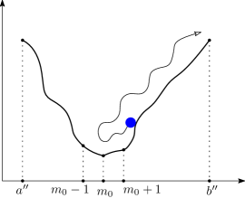
Figure 4: Escaping from a potential well.

Let us now explain why the expected time to go out of a potential well should be of order of exponential of its depth. Consider the situation depicted in Figure 4: ${\widehat{V}}(a^{\prime\prime})={\widehat{V}}(b^{\prime\prime})$, $m_{0}$ is where the minimum of ${\widehat{V}}$ on the interval $[a^{\prime\prime},b^{\prime\prime}]$ is attained, and, for the sake of cleanness, let us also suppose that ${\widehat{V}}(m_{0}\pm 1)-{\widehat{V}}(m_{0})$ are bounded away from $0$.

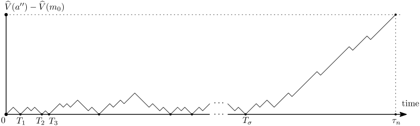
Figure 5: Calculating the distribution of the time to escape from a potential well (the vertical coordinate represents the “height” of the walk above ${\widehat{V}}(m_{0})$ with respect to the potential).

Then, the idea is to consider excursions of the Markov chain out of $m_{0}$ before hitting $\{a^{\prime\prime},b^{\prime\prime}\}$, i.e., climbing to the level ${\widehat{V}}(a^{\prime\prime})-{\widehat{V}}(m_{0})$ potential-wise (it should be noted that, in general, analysis of excursions is a very common approach when studying random walks). Let $\sigma$ be the number of those excursions, and $T_{1},T_{2},\ldots,T_{\sigma}$ be the time moments when the process is at $m_{0}$ (see Figure 5). Using Lemma 2.1, we obtain that, up to factors of a smaller order,

$${\mathbb{P}}_{m_{0}\pm 1}[\tau_{\{a^{\prime\prime},b^{\prime\prime}\}}<\tau_{m_{0}}]\approx e^{-({\widehat{V}}(a^{\prime\prime})-{\widehat{V}}(m_{0}))}.$$

This implies that the number of excursions $\sigma$ has approximately Geometric (and therefore approximately Exponential) distribution with mean around $e^{({\widehat{V}}(a^{\prime\prime})-{\widehat{V}}(m_{0}))}$; therefore, the expected value of $T_{\sigma}$ itself should be of order $e^{({\widehat{V}}(a^{\prime\prime})-{\widehat{V}}(m_{0}))}$ as well (because it is roughly $\sigma$ times the mean excursion length). We also need to argue that the length of the last excursion (from $m_{0}$ to $\{a^{\prime\prime},b^{\prime\prime}\}$) is typically negligible compared to $T_{\sigma}$. To see that, note that it is a trajectory of a conditioned (on the event $\{\tau_{\{a^{\prime\prime},b^{\prime\prime}\}}<\tau_{m_{0}}\}$) random walk, the so-called Doob’s $h$-transform of the original one, see e.g., Section 4.1 of [59] and also Exercise 4.58 of [66]. Essentially, it will behave as a random walk with inverted drift (i.e., towards the interval’s extremes), so it will typically have a length that does not exceed much in the order of magnitude the length of the interval $[a^{\prime\prime},b^{\prime\prime}]$; therefore, it will be typically negligible compared to $e^{({\widehat{V}}(a^{\prime\prime})-{\widehat{V}}(m_{0}))}$.

Now, with Claim 2.6 to hand, we can explain how the random walk on the above potential will typically behave. Of course, we assume that the size of the interval $[a,b]$ is large.

Assume that the random walk on Figure 6 starts somewhere near site $a$ (that is, “on top” of the potential). It will quickly come to the first metastable state (the leftmost potential well on Figure 6), and then spend roughly $e^{h_{1}}$ time there. Then, eventually, it will overcome the potential wall separating the first potential well from the second one, and then spend around $e^{h_{2}}$ time there (that would be the second metastable state of the process). Then, finally, it will climb the second wall of height $h_{2}$ and come to the deepest potential well (the ground state). After that, essentially, it will stay there (of course, very occasionally it will go back to the metastable states since it is a finite Markov chain, but the time spent there would be negligible in comparison to the time spent in the ground state).

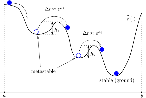
Figure 6: The metastability phenomenon, and time spent in metastable states.

The term “metastable state” thus means a state of the system which is not the one where the system passes the majority of the time in the long run (which would be around the global minimum of the potential), but where the system still spends quite a long time before finding its way out of there.

In general, metastability is a ubiquitous phenomenon in the context of statistical physics and stochastic processes; a complete overview of the relevant literature would be impossible here, but let us refer to [12, 11, 17, 33, 43, 56, 57] for a start. We mention also that this process of going from one metastable state to the next one is sometimes referred to as aging in the literature, see e.g., [26, 30].

Now, we return to the majority dynamics model of the previous section, but this time with Byzantine nodes. Fix a positive number $q\in(0,\tfrac{1}{2})$. We will now assume that, among those $n$ nodes, $(1-q)n$ are honest (i.e., they follow the prescribed protocol), and $qn$ are Byzantine. In principle, the Byzantine nodes can behave in any matter; here we assume that they all are controlled by a single entity, called the adversary. This entity is able to know the current state of the system; i.e., the adversary is omniscient. Let us warn the reader already at this point that the adversary can adopt a multitude of different strategies – these are, roughly, the “behaviors” that the adversary uses to achieve its goals. These goals may be, for example, to delay the consensus among the honest nodes, or to prevent it from occurring altogether by having different nodes finalize on different opinions, or to have some nodes reach their final opinion while keeping the others undecided.

Let us consider a very simple adversarial strategy: “Help the weakest”. That is, when queried, the adversarial nodes will always vote on the less popular opinion among the honest nodes. The goal now is to try to analyze the system similarly to the previous section, via a one-dimensional nearest-neighbor random walk.

Denote by ${\widetilde{X}}_{k}$ be the number of honest nodes with opinion $1$ at time $k$. Byzantine nodes have no real opinions, and if a Byzantine node is selected, then the state of the system will not change. Let us assume ${\widetilde{X}}_{k}=m$, and consider the following two cases.

Case 1: $m\leq\tfrac{(1-q)n}{2}$.

In this case, any Byzantine node, if queried, will vote for $1$. So, the number of $1$-opinions among three independently chosen nodes will have the Binomial$\big{(}3,\frac{m}{n}+q\big{)}$ distribution. Then, if one of the $m$ honest opinion-$1$ nodes was selected (which happens with probability $\frac{m}{n}$), it will switch its opinion to $0$ with probability $\big{(}1-\frac{m}{n}-q\big{)}^{3}+3\big{(}1-\frac{m}{n}-q\big{)}^{2}\big{(}\frac{m}{n}+q\big{)}$; likewise, if an honest node with current opinion $0$ was selected (which happens with probability $1-q-\frac{m}{n}$), it will switch its opinion to $1$ with probability $\big{(}\frac{m}{n}+q\big{)}^{3}+3\big{(}1-\frac{m}{n}-q\big{)}\big{(}\frac{m}{n}+q\big{)}^{2}$.

Case 2: $m>\tfrac{(1-q)n}{2}$.

In this case, a Byzantine node, if queried, will vote for $0$, and therefore the number of $1$-opinions among three independently chosen nodes has the Binomial$\big{(}3,\frac{m}{n}\big{)}$ distribution. Then, as before, if one of the $m$ honest opinion-$1$ nodes was selected, it will switch its opinion to $0$ with probability $\big{(}1-\frac{m}{n}\big{)}^{3}+3\big{(}1-\frac{m}{n}\big{)}^{2}\big{(}\frac{m}{n}\big{)}$; if an honest node with current opinion $0$ was selected, it will switch its opinion to $1$ with probability $\big{(}\frac{m}{n}\big{)}^{3}+3\big{(}1-\frac{m}{n}\big{)}\big{(}\frac{m}{n}\big{)}^{2}$.

Note, in particular, that $0$ and $(1-q)n$ are not absorbing states anymore — because even if all the honest nodes agree, there is a chance that the selected honest node will choose at least two Byzantine ones for opinions and those will convince it to switch.

That is, we find that the process $({\widetilde{X}}_{k},k\geq 0)$ is a (one-dimensional) random walk on $\{0,\ldots,(1-q)n\}$, and on ${\widetilde{X}}_{k}=m$ we have

$${\widetilde{X}}_{k+1}=\begin{cases}m-1,&\text{with probability }{\tilde{p}}_{m},\\ m+1,&\text{with probability }{\tilde{q}}_{m},\\ m,&\text{with probability }{\tilde{v}}_{m}=1-{\tilde{p}}_{m}-{\tilde{q}}_{m},\end{cases}$$ (16)

where

$${\tilde{p}}_{m} =\begin{cases}\tfrac{m}{n}\big{(}\big{(}1-\tfrac{m}{n}-q\big{)}^{3}+3\big{(}\tfrac{m}{n}+q\big{)}\big{(}1-\tfrac{m}{n}-q\big{)}^{2}\big{)},&\text{ if }m\leq\tfrac{(1-q)n}{2},\\ \tfrac{m}{n}\big{(}\big{(}1-\tfrac{m}{n}\big{)}^{3}+3\tfrac{m}{n}\big{(}1-\tfrac{m}{n}\big{)}^{2}\big{)},\vphantom{\displaystyle\sum^{a}}&\text{ if }m>\tfrac{(1-q)n}{2},\end{cases}$$

$${\tilde{q}}_{m} =\begin{cases}\big{(}1-\tfrac{m}{n}-q\big{)}\big{(}\big{(}\tfrac{m}{n}+q\big{)}^{3}+3\big{(}\tfrac{m}{n}+q\big{)}^{2}\big{(}1-\tfrac{m}{n}-q\big{)}\big{)},&\text{ if }m\leq\tfrac{(1-q)n}{2},\\ \big{(}1-\tfrac{m}{n}-q\big{)}\big{(}\big{(}\tfrac{m}{n}\big{)}^{3}+3\big{(}\tfrac{m}{n}\big{)}^{2}\big{(}1-\tfrac{m}{n}\big{)}\big{)},\vphantom{\displaystyle\sum^{a}}&\text{ if }m>\tfrac{(1-q)n}{2}.\end{cases}$$

We then define the potential ${\widetilde{V}}$ analogously to (3) (with ${\tilde{p}}$’s and ${\tilde{q}}$’s on the place of $p$’s and $q$’s).

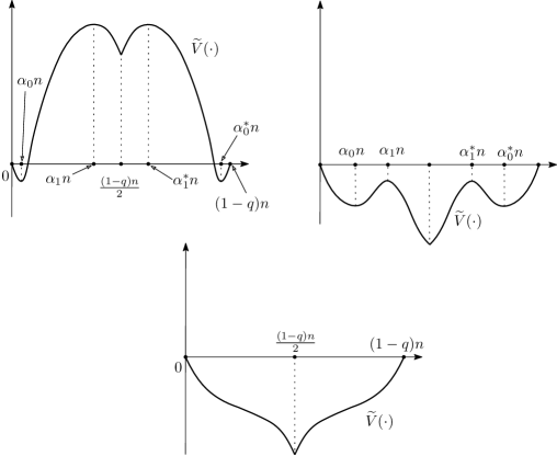
Figure 7: The potential profile for the majority dynamics with Byzantine nodes: with $q<0.09029$ (top left), $0.09029<q<\frac{1}{9}$ (top right), $q>\frac{1}{9}$ (bottom).

By examining the above transition probabilities, one can show that ${\widehat{V}}$ looks as shown in Figure 7. Indeed, let us try to find out for which values of $m\leq\tfrac{(1-q)n}{2}$ the drift ${\tilde{q}}_{m}-{\tilde{p}}_{m}$ would become $0$ — these would correspond to the “flat points” (typically minimums or maximums) of the potential ${\widehat{V}}$. To this end, we abbreviate $\alpha=\tfrac{m}{n}$, and solve the equation

$$\alpha\big{(}(1-\alpha-q)^{3}+3(\alpha+q)(1-\alpha-q)^{2}\big{)}=(1-\alpha-q)\big{(}(\alpha+q\big{)}^{3}+3(\alpha+q)^{2}(1-\alpha-q)\big{)}.$$

Note that one can divide both sides by $(1-\alpha-q)$ and then cancel the $\alpha^{3}$ terms. The two real roots that we are interested in are

$$\alpha_{0}(q) =\tfrac{1}{4}\Big{(}1-\sqrt{1-\tfrac{8q}{1-q}}\Big{)}-q,$$

$$\alpha_{1}(q) =\tfrac{1}{4}\Big{(}1+\sqrt{1-\tfrac{8q}{1-q}}\Big{)}-q,$$

which only exist for $q\in(0,\frac{1}{9}]$. One can also obtain that

$$\alpha_{0}(q)=3q^{2}+O(q^{3})\text{ and }\alpha_{1}(q)=\tfrac{1}{2}-2q+O(q^{2})\quad\text{ as }q\to 0.$$ (17)

Define also the “symmetric” points $\alpha^{*}_{0}(q)=1-q-\alpha_{0}(q)$ and $\alpha^{*}_{1}(q)=1-q-\alpha_{1}(q)$. To be able to distinguish between the situations in the second and third pictures in Figure 7, it is then important to be able to compare the values of ${\widehat{V}}\big{(}\alpha_{0}(q)\big{)}$ and ${\widehat{V}}\big{(}\tfrac{(1-q)n}{2}\big{)}$; for this, we essentially need to know the sign of the sum $\sum_{m=n\alpha_{0}(q)}^{(1-q)n/2}\log\tfrac{{\hat{p}}_{m}}{{\hat{q}}_{m}}$. We can approximate the sum with the integral and note that the equation (in $q$)

$$\int\limits_{\alpha_{0}(q)}^{\frac{1-q}{2}}\log\frac{s((1-s-q)^{2}+3(s+q)(1-s-q))}{(s+q)^{3}+3(s+q)^{2}(1-s-q)}\,ds=0$$ (18)

has the solution $q^{*}\approx 0.09029$ (obtained numerically). Therefore, roughly at $q^{*}$ there should occur the phase transition between the top left and top right pictures in Figure 7.

The key difference with the non-Byzantine case (recall Figure 2) is that now in this ${\widetilde{V}}$-picture there are possibly three potential wells. Claim 2.6 (iv) tells us that, in a situation like that, the random walker will typically need quite a lot of time to escape from the well.

For the 3-choice majority dynamics with the “help the weakest” adversarial strategy, we therefore find that

• with $q<q^{*}$, there are three locally attractive states - two pre-consensus ones, and one “balanced” (i.e., “$50/50$”); but the pre-consensus states are ground (that is, “stronger”; i.e., in the long run, the system will “prefer” to stay in those due to Claim 2.6 (iii));

• with $q^{*}<q<\frac{1}{9}$, those three states remain, but now the balanced one is the ground state (so the system might spend some time in a pre-consensus state, but in the long run it will fall to the ground state, again due to Claim 2.6 (iii));

• with $q>\frac{1}{9}$, there are no pre-consensus states (so the system just goes to the “balanced” ground state from anywhere).

Let us discuss the $q<q^{*}$ situation (the top left picture in Figure 7) in a little more detail. By Claim 2.6 (ii) (in fact, Lemma 2.1 applied to the present situation), if the process starts sufficiently out of the interval $[\alpha_{1}(q)n,\alpha^{*}_{1}(q)n]$ (i.e., out of the central potential well), it will go to the corresponding pre-consensus state with probability exponentially close to $1$. Then, an important practical observation is that, if in a pre-consensus state, the honest nodes have a way to figure out the preferred state of the system, e.g., by averaging over last $N$ responses received, with a very high probability, a significant majority will choose the same as the preferred state. This can be seen as a “positive” result: even with Byzantine nodes, in the case where the initial opinion configuration is sufficiently away from the “balanced” situation, we are able to achieve practical consensus with high probability. However, later we will see that the presence of the central potential well does pose some very serious problems in practice.

Let us now ask the following question: what if we slightly increase the communication complexity by asking $k>3$ nodes for opinions, instead of just three? What are the benefits of this increase? For convenience, let us assume that $k$ is odd, so that draws are not possible. First, let us show that the distance from total consensus to the bottoms of the two pre-consensus wells will be of order $q^{\tfrac{k+1}{2}}$ as $q\to 0$. Recall (17): this agrees with the fact that $\alpha_{0}(q)\asymp q^{2}$ with $k=3$. Indeed, assume that the system (i.e., the number of honest nodes with current opinion $1$) is currently in the state around $m=Cq^{\tfrac{k+1}{2}}n$. Then, the probability that an honest node with opinion $1$ is selected is approximately $Cq^{\tfrac{k+1}{2}}$, and then it will flip its opinion with probability close to $1$ (since the proportion of the nodes who would respond $0$ when chosen will be around $1-q-Cq^{\tfrac{k+1}{2}}>\tfrac{1}{2}$, so the fact that the Binomial distribution becomes more concentrated as $k$ increases will take care of that). On the other hand, the probability that an honest node with opinion $0$ is selected is around $1-q-Cq^{\tfrac{k+1}{2}}$, and then it will flip its opinion with probability around $c^{*}q^{\tfrac{k+1}{2}}$ (this can be seen from the explicit formula for the Binomial probability distribution). Then, we see that (up to terms of smaller order, and keeping the notations ${\tilde{p}}_{m},{\tilde{q}}_{m}$ for the case of $k$ chosen nodes) $\frac{{\tilde{p}}_{m}}{{\tilde{q}}_{m}}\approx\tfrac{C}{c^{*}}$, so the bottom of the left pre-consensus well will be around $c^{*}q^{\tfrac{k+1}{2}}n$. That is, increasing $k$ indeed permits us to approximate the pre-consensus to the consensus, thus also making it easier to design the local decision rules used by the honest nodes to finalize their opinions.

However, let us show that the width or size of the central potential well will not tend to zero (in fact, it will always remain at least $qn$). Indeed, notice first that if the state of the system is close to $\tfrac{(1-2q)}{2}n$, then (since the Byzantine nodes would vote for $1$) a chosen peer would vote for $0$ or $1$ roughly with equal probabilities; however, since the probability of selecting an honest node with opinion $1$ is significantly less than the probability of selecting an honest node with opinion $0$, the process will have a drift to the right (meaning that it is inside the central potential well). For completeness, observe also that for a fixed $a<\tfrac{(1-2q)}{2}$ one can find a large enough $k$ such that $an$ is out of the central well. Indeed, the probability that a randomly chosen node would vote for $1$ would then be $a+q<\tfrac{(1-2q)}{2}+q=\tfrac{1}{2}$, and then it is clear that the probability that a Binomial$(k,a+q)$ random variable does not exceed $\tfrac{k-1}{2}$ can be made as small as we want by the choice of $k$. This shows that, as we grow $k$, the central potential well “shrinks towards” $\big{[}\tfrac{(1-2q)}{2}n,\tfrac{1}{2}n\big{]}$, but that interval (of length $qn$) is always a part of it.

To finalize this subsection on a not-so-optimistic note, observe that we have analyzed only one adversarial strategy: the “help-the-weakest”. This point also explains why analyzing the system via simulations is not a straightforward task — these need to be performed for any adversarial strategy, and there are infinitely many of them. It is also necessary to mention that, in principle, with more complicated adversarial strategies or node’s finalizations rules the process may not even be a Markov chain which would make its analysis much more difficult.

2.3 Obstacles on the road to consensus: the curse of metastability

We have just seen the most immediate consequence of having Byzantine nodes: some natural adversarial strategies can lead to metastable states, where, due to Claim 2.6 (iv), the process can spend quite a lot of time (exponential in the number of Byzantine nodes provided that they make a positive fraction of the totality, which could mean essentially forever in practice).

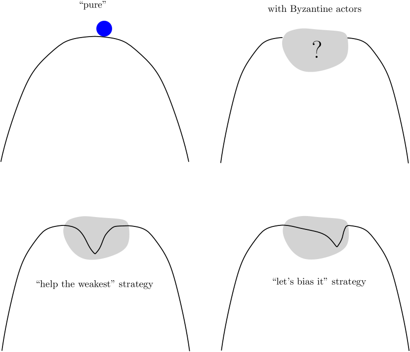
Figure 8: Majority dynamics with Byzantine actors: the curse of metastability.

The situation is summarized in Figure 8 (we disregard the pre-consensus potential wells there, as they may be made small by the choice of $k$, and, in any case, the honest nodes are able to make the correct decision while the process is spending time in those). Essentially, in the all-honest situation (top left picture), regardless of the starting position, the process will quickly end up in one of the two consensus states. However, with Byzantine actors (top right picture), the adversary has a “region of control” (indicated by the big question mark) where it is able to dictate what the system will do. For example, for the natural “help the weakest” strategy (discussed in detail in Section 2.2) the potential profile is as in the bottom left picture, meaning that, when started not far away from the balance, the process is likely to spend a lot of time near the “exactly balanced” situation. As noted at the end of the previous section, other adversarial strategies are possible, for example, the one on the bottom right part of Figure 8. There, the adversary prefers to “bias” the overall opinion counts slightly towards one of the extremes (while still remaining in its region of control). This approach might make sense because it would increase the probability that, during that long time spent in the potential well, some of honest nodes would already finalize on that “slightly preferred” opinion because their finalizations rules would be triggered by some “improbable” events (and then the adversary would even be able to sway the consensus to the other side).

The last point highlights an important (and perhaps not a-priori clear) problem: the existence of metastable states not only compromises liveness but also casts doubts on the system’s safety. The reason is that, as it sometimes happens with large stochastic systems, improbable things can happen if one waits for a really long time. Since the local finalization rules used by the nodes are usually publicly known, the adversary may try using that knowledge to create conditions whereby finalization still might occur during a sufficiently long time interval while the process is still within the adversary’s region of control. To assess the risk of such a development, one would need to employ some entropy-versus-energy-type arguments (that, basically, compare the inverse probability of an “improbable” event to the number of “tries” when that event might occur), and the question of optimizing over adversary’s strategies would stand even then.

In view of the above, a natural idea would be to set some limit on the time to achieve consensus, i.e., if a transaction’s status is still undecided after some fixed time $t_{\text{max}}$, then just consider this transaction invalid, i.e., set its status to $0$. However, this can be dangerous, because some nodes would finalize on $1$ just barely while others just barely not (and therefore set the final opinion to $0$ according to that rule), with a non-negligible probability (especially if the adversary stops messing with the system “just before” the limit time $t_{\text{max}}$ elapses). Another natural idea would be to introduce some tie-breaking rule: based on the information available in the system, the nodes would spontaneously switch to one of the opinions in case the balanced state persists for too long. If enough honest nodes do that approximately at the same time, the system may be pushed towards one of the extremes. This idea certainly deserves further research; however, this sort of metastability-breaking is not easy to achieve when the adversary has (almost) full information: the adversary would be facing a sort of stochastic control problem, and might be able to influence the state of the system (i.e., “adjust the controls”) in such a way that not enough honest nodes are able to take that sort of coordinated action, and therefore the split would persist. In the next section, however, we will describe a metastability-breaking mechanism that uses external randomness (which cannot be predicted by the adversary) and show that it indeed makes the system achieve consensus in a well-controlled way.

In any case, to explore the attacks outlined in this section, the adversary has to be “smart” (i.e., adjust its behavior to the state of the honest nodes in perhaps a non-trivial way) and well-connected (to be able to know the state at least with some degree of precision). It is clear that the system will not “break by itself” (with the adversary not abiding by the rules but just doing random things); on the other hand, it is also clear that a smart-and-well-connected adversary can disrupt the system to a considerable extent, at least in theory. For sure, one has to bear in mind that the adversary’s omniscience assumption is an idealized one, and that in a practical system from the adversary’s point of view there will be some “natural randomness” (stemming from, e.g., differences in nodes’ local perceptions, fluctuations in message delivery times, own limitations in connectivity and processing power that would prevent the adversary from catching up with the rest of the network, and so on) that the adversary cannot predict/control. In principle, this “adversarial unawareness” could also act as a metastability breaker, but one would have to exercise quite some caution when relying on it. The problem is that there will likely be a sharp phase transition with respect to the amount (whatever it means) of that randomness: too much “fog of war” would prevent the attacker from maintaining metastable states, but a small amount of it would mean that the above-discussed potential wells are still present and therefore the adversary would be still in control (in the situation when opinions are split). In any case, as we have already mentioned, it is not necessarily clear how to define/measure/control this factor and what guarantees there are that no adversary would be able to become sufficiently powerful in the foreseeable future.

One example of a paper that could have benefited from the analytic tools and arguments outlined here is [65] (we cite also [64], which contains more technical details). As argued above, to access the protocol’s safety it is not enough to just prove that it will converge to consensus starting from an already sufficiently biased situation (i.e., sufficiently out of the central potential well, in the case of the “help the weakest” adversarial strategy; admittedly, even for this situation the arguments in these papers are far from convincing). There is no attempt to approach it via the above-mentioned “entropy-versus-energy” arguments, which, in particular, would be important in the case of the above-mentioned “let’s bias it” strategy. The authors of the aforementioned papers also claim that they have studied their model via simulations, but it is not completely clear which adversarial strategies were considered, and why those strategies would be optimal from the adversary’s point of view. It is also unfortunate that these papers do not contain explicit estimates on the probabilities of “bad” events; as argued in this section, in such circumstances it is hardly possible to access if the system can scale well. As consensus protocols play a prominent role in every distributed ledger’s safety, the authors want to stress the need to approach any “solution” without a metastability-breaking mechanism with skepticism.

3 FPC: breaking metastable states

In this section, we describe a recent solution, the fast probabilistic consensus (FPC) introduced in [60]. FPC breaks metastable states with the use of external randomness.

The use of common external randomness necessitates a change of the dynamics. We no longer ask nodes to update their opinions one by one, but instead ask them to update their opinions synchronously in rounds. As previously noted, it is possible that such a synchronous model could in theory be analyzed as the asynchronous toy model, but the analysis would be much more technical. In fact, the corresponding random walk would not only be able to jump steps of length $1$, but its step distribution may be of full support.

As in the previous toy model, the basic feature of FPC is that, in each round, each node queries a random subset of known peers of size $k$ about their current opinion. We allow $k$ to be relatively large, e.g., $k=25$, but still assume that $k\ll n$. Once a node receives the answers to its queries, it updates its opinion. This continues until a local stopping rule is satisfied, as discussed in the previous section.

On a high level, the main idea of the FPC can be explained in the following way. As we have seen in Section 2, if the adversary is able to know (at least with some precision) what the state of the honest part of the system is and is able to predict the honest nodes’ behavior, then it may be able to seriously interfere with the system.

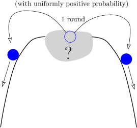
Figure 9: FPC: defeating the metastability with round-based common random thresholds.

On the other hand, assume that the decision rule used by the honest nodes to choose the preferred opinion is unpredictable; that is, cannot be known in advance by the adversary. In this case, the result is illustrated in Figure 9: there is a good chance that, in just one round, the situation completely escapes the adversary’s control (the system jumps into a pre-consensus state from where it will quickly converge to consensus regardless of the adversary’s actions). This unpredictability is achieved by using a sequence of common random numbers, which are either provided by an external source or generated by the nodes of the system themselves (or, in practice, by a subcommittee of those), see e.g., [16, 44, 58, 67, 70, 73].

3.1 Notation and description of the protocol

Every node $i$ starts with an initial state or opinion $s_{i}(0)\in\{0,1\}$. We update every nodes opinion at each round, and we note $s_{i}(t)$ for the opinion of the node $i$ at time $t\in\mathbb{N}$. At each time step each node chooses $k$ (random) neighbors $C_{i}$, queries their opinions, and calculates

$$\eta_{i}(t+1)=\frac{1}{k_{i}(t)}\sum_{j\in C_{i}}s_{j}(t),$$

where $k_{i}(t)$ is the number of replies at time $t$.

It is possible that not all nodes respond and one can set the value for $s_{j}(t)$ in the case of no response to $0$, $1$ or NA. This case is similar to a proportion of nodes being faulty and can be modeled through strategies for malicious nodes introduced in Section 3.2.

In FPC the first round may be different from the subsequent rounds. Any binary decision, as in statistical test theory or binary classification, gives rise to two possible errors. In many applications, the two possible errors are asymmetric in the sense that one error is more severe than the other. Choosing the threshold of the first voting round differently allows the protocol to include this kind of asymmetry. Let $U_{1}$ be a uniform distributed random variable $\mathrm{Unif}([a,b])$, for $0\leq a\leq b\leq 1$, and $U_{t},t=1,2,\ldots$ be uniform random variables with law $\mathrm{Unif}([\beta,1-\beta])$ for some parameter $\beta\in[0,1/2]$. We assume the random variables $(U_{t})_{t\geq 1}$ to be independent.

The update rules are now given inductively for $t\geq 1$ by

$$s_{i}(t+1)=\left\{\begin{array}[]{ll}1,\mbox{ if }\eta_{i}(t+1)>U_{t},\\ 0,\mbox{ if }\eta_{i}(t+1)<U_{t},\\ s_{i}(t),\mbox{ otherwise.}\end{array}\right.$$ (19)

The essential ingredient of FPC, compared to previous voting models is that the thresholds $U_{t}$ are random. The usual majority dynamics would compare the $\eta$’s against the deterministic threshold $\tfrac{1}{2}$.

Nodes have to decide locally when to stop the protocol and no longer update their opinions. One possibility of such a local stopping rule is that a node stops querying other nodes and finalizes its opinion if it did not change its opinion for the last $\ell$ rounds. In the original paper [60] there is also a cooling-off period of $m_{0}$ rounds after which the above rule starts to be applied. A node will continue to answer queries until some maximal number of rounds, say $\Delta$, is attained.

We will distinguish in this exposition between two different ways a voting-based consensus protocol can fail.

1. Termination failure: We say the protocol suffers a termination failure if some node did not stop querying before the maximal number of rounds.

2. Agreement failure: We say the protocol suffers an agreement failure if two honest nodes terminate with different final opinions.

We say that the protocol terminates in agreement, if there are neither agreement nor termination failures.

3.2 Threat model

Byzantine infrastructures and attack strategies can be very diverse. We assume that adversarial nodes can exchange information freely between themselves and can agree on a common strategy. In fact, they all may be controlled by a single individual or entity.

As in Section 2.2, we suppose that $qn$ nodes are adversarial for some $q\in[0,1]$. The remaining $(1-q)n$ nodes are honest, i.e., they follow the recommended protocol.

With respect to the behavior of the adversarial nodes, we distinguish three cases:

• Cautious adversary: Any adversarial node responds the same value to all the queries it receives in that round. The adversary knows the opinions of the honest nodes in the previous rounds.

• Semi-cautious adversary: Any adversarial node does not give contradicting responses (i.e., $0$ to one node and $1$ to another node in the same round) but does not have to answer all queries. The adversary knows the opinions of the honest nodes in the previous rounds.

• Berserk adversary: Any adversarial node may respond differently to different queries in the same round. At each moment of time, the adversary is not only aware of the current opinions of all honest nodes but may also know which nodes query which other nodes.

The berserk adversary is the worst-case scenario; we pose no limitation on the node’s behavior and allow it to be omniscient, i.e., it knows all information that exists until now. However, it is not prescient nor possesses prior knowledge or influence on the random threshold.

Let us explain why the adversary may choose to be cautious or semi-cautious. We assume that nodes have identities and sign all their messages; this way, one can always prove that a given message originates from a given node. Now, if a node is not cautious, this may be detected by the honest nodes, e.g., two honest nodes may exchange their query history and verify that the same node passed contradicting information to them. In such a case, the offender may be penalized by the honest nodes. For example, the nodes who discovered the fraud would pass that information along with the relevant proof and the other honest nodes would stop querying this particular node.

The semi-cautious adversary has slightly more freedom in lying (in fact, in not saying anything) than a cautious adversary. We will see later that this additional freedom has an impact on the security of the system.

3.3 Theoretical results

The theoretical results on FPC found in [60] are obtained under various assumptions. We discuss the necessity of these assumptions in Section 3.5. In this section we assume that every node knows all other participants, that it can directly query any other node, and that honest nodes always reply in due time. In addition, we assume the existence of a common source of randomness that delivers a fresh random threshold in every round.

A complete formulation and proof of the theoretical results of [60] would require some more notations and end up being rather technical. For this reason, we present several results from [60] that stand by way of example for the more general and more technical results.

Let us define two events relative to the final consensus value:

$$H_{i}=\{\text{all honest nodes eventually reach final opinion }i\},$$ (20)

$i=0,1$. Thus, the union $H_{0}\cup H_{1}$ stands for the event that all honest nodes agree on the same value, i.e., that the consensus was achieved.

Let $\mathcal{N}$ be the number of rounds until all honest nodes achieve their final opinions. In the following result (which is a corollary of Theorems 4.1 and 6.1 of [60]), we obtain a lower bound on the probability of the event $(H_{0}\cup H_{1})\cap\{\mathcal{N}\leq m_{0}+\ell\}$. This event means that the consensus was achieved in the shortest possible time $m_{0}+\ell$.

Theorem 3.1.

• In the case of a cautious adversary, assume that $q<1/2$. Then, for any fixed $\beta\in(q,1/2)$ we have, with $c_{0,1,2}>0$ depending on $\beta$ and $q$

  $${\mathbb{P}}\big{[}(H_{0}\cup H_{1})\cap\{\mathcal{N}\leq m_{0}+\ell\}\big{]}$$

  $$\geq 1-c_{0}n\ell\exp(-c_{1}k)-\exp(-c_{2}m_{0}\ln k).$$ (21)

• In the case of a semi-cautious adversary, assume that $q<\frac{3-\sqrt{5}}{2}$. Then, for any fixed $\beta\in(q,\frac{1-q}{2-q})$ we have, with $c_{0,1,2}>0$ depending on $\beta$ and $q$

  $${\mathbb{P}}\big{[}(H_{0}\cup H_{1})\cap\{\mathcal{N}\leq m_{0}+\ell\}\big{]}$$

  $$\geq 1-c_{0}n\ell\exp(-c_{1}k)-\exp(-c_{2}m_{0}).$$ (22)

• In the case of a berserk adversary, assume that $q<1/3$. Then, for any fixed $\beta\in(q,\frac{1-q}{2})$ we have, with $c_{0,1,2}>0$ depending on $\beta$ and $q$

  $${\mathbb{P}}\big{[}(H_{0}\cup H_{1})\cap\{\mathcal{N}\leq m_{0}+\ell\}\big{]}$$

  $$\geq 1-c_{0}n\ell\exp(-c_{1}k)-\exp(-c_{2}m_{0}).$$ (23)

It is also important to observe that the above theoretical estimates (as well as those of [60]) are not necessarily sharp; this explains why we keep the possibility of using a generic $\ell$ even though $\ell=1$ would be the most “favorable” for the above estimates (21)–(22); in practice a higher value of $\ell$ may work better (as shown in [15]).

Asymptotic results are of interest in evaluating the scalability of the protocol. In addition, the next corollary gives more quantitative details on the probability of terminating in an agreement.

Corollary 3.2.

Let $\beta=1/3$ and $\ell$ be some constant. We assume that the proportion of Byzantine nodes $q$ is acceptable, i.e., less than $1/2$ for the case of a cautious adversary, less than $\frac{3-\sqrt{5}}{2}$ for a semi-cautious adversary, or less than $1/3$ for the case of a berserk adversary. Then, there exists some constant $C$ such that for $k=C\log n$ and

• $m_{0}=O\big{(}\frac{\ln n}{\ln\ln n}\big{)}$ for the cautious adversary,

• $m_{0}=O(\ln n)$ for the semi-cautious and berserk adversary,

the probability of terminating in agreement is at least $1-\varepsilon(n)$, where $\varepsilon(n)$ is polynomially small in $n$ (i.e., $\varepsilon(n)=O(n^{-h})$ for some $h>0$, and this $h$ can be made arbitrarily large by choosing a suitable $C$).

In particular, the overall communication complexity is at most $O\big{(}\frac{n\ln^{2}n}{\ln\ln n}\big{)}$ for a cautious adversary and $O(n\ln^{2}n)$ for a berserk one.

Now, we outline the strategy of the proof of the above results. Let ${\hat{p}}_{m}$ be the proportion of $1$-opinions among the honest nodes after the $m$th round. Let us define the random variable

$$\Psi=\min\big{\{}m\geq 1:{\hat{p}}_{m}\leq\tfrac{\beta-q}{2(1-q)}\text{ or }{\hat{p}}_{m}\geq 1-\tfrac{\beta-q}{2(1-q)}\big{\}}$$ (24)

to be the round after which the proportion of $1$-opinions among the honest nodes either becomes “too small”, or “too large”. The idea is that, when $\Psi$ happens, it then becomes extremely likely that all $(1-q)n$ honest nodes will maintain the same opinion (which will be $0$ if the first condition in (24) occurs or $1$ if the second one does) during the $\ell$ consecutive rounds needed for reaching consensus. It is here that the fact that $q<1/2$ is important: when the honest nodes are almost in agreement, the adversarial nodes do not have the necessary voting power to convince them otherwise. In fact, it is also important that the parameter $\beta$ is chosen in such a way that $\beta>q$: in the situation when almost all honest nodes agree, the adversary must not be able to reach the interval $[\beta,1-\beta]$ where the decision thresholds live. As the reader probably figured out, the first negative term in the right-hand sides of (21)–(22) correspond to the probability that at least one node of the system “jumps out” of the consensus state during the $\ell$ finalization rounds (in particular, the factor $n\ell$ there comes from the union bound). We do not elaborate further in this paper; a rigorous derivation of the corresponding bounds was done in [60].

Now let us explain the origin of the second negative terms in the right-hand sides of (21)–(22); those come from the tail estimates on $\Psi$ – the probabilities that $\Psi$ did not happen during the $m_{0}$ preliminary rounds. In the following, we elaborate on this for cautious, berserk, and semi-cautious adversaries (and also explain the reasoning behind the corresponding security thresholds $1/2$, $1/3$, and $\varphi^{-2}=\frac{3-\sqrt{5}}{2}$). To simplify the arguments, we assume that the honest nodes’ opinions are roughly equally split (that is, approximately $\frac{1}{2}(1-q)n$ of those have current opinion $0$ and approximately $\frac{1}{2}(1-q)n$ have current opinion $1$), and the adversary is attempting to maintain this 50/50 split.

Cautious adversary

This is the simplest case since the adversary essentially has to choose the opinions of the nodes it controls beforehand; this in turn means that the expected proportions of $1$-opinions that honest nodes receive will be the same, and therefore the actual proportions of $1$-opinions they receive will likely be distributed on an interval of length $O(k^{-1/2})$ because of the Central Limit Theorem (we refer the reader to Figure 2 of [60]). To maintain the opinions split, the next (not yet known to the adversary) decision threshold has to be in that interval; this happens with a probability of order $k^{-1/2}$. Therefore, this explains the second negative term in the right-hand side of (21) (note that $(ck^{-1/2})^{m_{0}}=\exp(-\frac{1}{2}m_{0}(\ln k-2\ln c))$). Note also that here we do not need further restrictions on $q$ (other than $q<1/2$).

Berserk adversary

In this case, the adversary can adopt for example the following strategy: feed $0$-opinions to one-half of the honest nodes, and $1$-opinions to the other half. Then the honest nodes from the first half will receive around $\frac{1}{2}(1-q)$ proportion of $1$s (because they will only receive $1$-opinions from honest nodes), while the proportion of $1$s that those from the second half will receive will be around $\frac{1}{2}(1-q)+q=\frac{1}{2}(1+q)$. Then, to assure that $\Psi$ happens with at least a positive constant probability, we need $[\frac{1}{2}(1-q),\frac{1}{2}(1+q)]$ to be a proper subset of $[\beta,1-\beta]$ (since in this case with uniformly positive probability the decision threshold will be outside of $[\frac{1}{2}(1-q),\frac{1}{2}(1+q)]$, and therefore most of the honest nodes will adopt the same opinion in the next round). This means that, besides the initial restriction $q<\beta$, we also need to have $\frac{1}{2}(1-q)>\beta$, that is, $\beta\in(q,\frac{1}{2}(1-q))$. The last interval must be nonempty meaning that $q<\frac{1}{2}(1-q)$, which is equivalent to $q<1/3$.

Semi-cautious adversary

Recall that we are assuming that the current opinions of honest nodes are roughly equally split; we will also consider only a symmetric adversarial strategy: $\frac{1}{2}qn$ adversarial nodes will answer $0$ or remain silent while the remaining $\frac{1}{2}qn$ adversarial nodes will answer $1$ or remain silent (the general case is treated in Section 6 of [60]). Let us see what happens if the adversary adopts a similar strategy as considered above for a berserk one: to half the honest nodes the adversarial nodes will answer $0$ (if possible) or remain silent, while to the other half they will answer $1$ (if possible) or remain silent. Note that a random query of any honest node will be answered with probability $1-q+\frac{q}{2}=1-\frac{q}{2}$ in this setup. Then, given that an honest node from the first half receives an answer, this answer will be

$$\begin{cases}0,&\text{with probability }\frac{\frac{1}{2}(1-q)+\frac{q}{2}}{1-\frac{q}{2}}=\frac{1}{2-q},\\ 1,&\text{with probability }\frac{\frac{1}{2}(1-q)}{1-\frac{q}{2}}=\frac{1-q}{2-q},\end{cases}$$

and, likewise, given that an honest node from the second half receives an answer, this answer will be $0$ with probability $\frac{1-q}{2-q}$ and $1$ with probability $\frac{1}{2-q}$. So, roughly speaking, the adversary can achieve the following: the proportion of $1$-opinions received by the honest nodes from the first half will be around $\frac{1-q}{2-q}$, while the proportion of $1$-opinions received by the honest nodes from the second half will be around $\frac{1}{2-q}$. Therefore, similarly to the berserk case, we need the interval $[\frac{1-q}{2-q},\frac{1}{2-q}]$ to be a proper subset of $[\beta,1-\beta]$ which (again, together with the condition $q<\beta$) shows that the inequality $q<\frac{1-q}{2-q}$ must hold. Solving this inequality for $q\in[0,1]$, we obtain $q<\frac{3-\sqrt{5}}{2}$.

Let us also comment on the cooling-off period $m_{0}$: it was initially introduced in [60] with the following idea in mind: let us first give some time to $\Psi$ to happen, and then the nodes can reach the consensus in safety. In fact, roughly the same asymptotic results as in Theorem 3.1 and Corollary 3.2 can be proved also for the protocol’s version with no cooling-off; specifically, for the probability ${\mathbb{P}}\big{[}(H_{0}\cup H_{1})\cap\big{\{}\mathcal{N}\leq\frac{3}{2}\ell\big{\}}\big{]}$ the same estimates with $m_{0}$ substituted to $\ell$ (and possibly different constants) will be valid. To see that, first observe that the probability that $\Psi$ does not happen during the first $\tfrac{\ell}{2}$ rounds will be at most $\exp\big{(}c\tfrac{1}{2}\ell\ln k\big{)}$ for the cautious adversary and at most $\exp\big{(}c\tfrac{1}{2}\ell\big{)}$ for the semi-cautious and berserk ones (recall the last terms in (21)–(23)). Then, every honest node would need to decide on the majority opinion between $\tfrac{\ell}{2}$ and $\ell$ consecutive times; the middle terms in the right-hand sides of (21)–(23) still are upper bounds to the probability that the above does not happen.

3.4 Numerical results

The theoretical results are strong in the sense that they cover all possible adversary strategies and that they give asymptotic results. However, the achieved bounds are not optimal and the actual performances of FPC seem to be much better. In this section, we highlight some results obtained by Monte-Carlo simulations that illustrate the performances of FPC and also indicate that most of the strict assumptions for the theoretical results can be considerably weakened. We also describe a concrete berserk strategy that is able to break the usual majority-dynamics without the random threshold.

FPC is governed by many parameters and allows users to adjust the protocol in many ways. In [52] various different parameter setting are studied with respect to the protocol performances. The authors of [52] proposed a simplified model and removed the randomness of the initial threshold and the cooling-off phase. While the theoretical results of [60] show that the cooling-off phase may reduce the minimum number of voting rounds required for termination, the asymptotic results in Corollary 3.2 states that $m_{0}$ can be chosen as $O(\log n)$. Moreover, the proof strategy in [60] and the discussion at the end of the previous section suggest that the theoretical results remain valid in the absence of the cooling-off phase. While in the original FPC, the initial threshold is randomly chosen in an interval $[a,b]$, we want to emphasize that the theoretical results in [60] remain valid for a deterministic threshold and that the randomness in the subsequent rounds is sufficient for the protocol’s robustness. For these reasons, we set in this section $a=b=\tau$.

As before, we assume that a proportion of $q\in[0,1)$ nodes are malicious and try to interfere with the protocol. As mentioned earlier we distinguish between different kinds of adversarial behavior. In the following, we give two explicit examples of possible adversary strategies.

Cautious strategy for agreement and termination failure

We consider the cautious strategy where the adversary transmits in round $t+1$ the opinion of the minority of the honest nodes of round $t$. This is the “help-the-weakest” strategy of Section 2.2. In [15] this strategy is dubbed the inverse vote strategy (IVS).

Berserk strategies for agreement and termination failure

We consider the berserk strategy known as maximal variance strategy (MVS). In this approach, the adversary waits until all honest nodes received opinions from all other honest nodes. The adversary then tries to subdivide the honest nodes into two equally sized groups of different opinions while trying to maximize the variance of the $\eta$-values (recall Section 3.1).

In order to maximize the variance, the adversary requires knowledge over the $\eta$-values of the honest nodes at any given time. The adversary then answers queries of undecided nodes in such a way that the variance of the $\eta$’s is maximized by keeping the median of the $\eta$’s close to $0.5$; we refer to [15] for a pseudo-code of the attack strategy. Intuitively, this strategy tries to make the central well in the upper left potential in Figure 7 as deep as possible.

The effectiveness of the random threshold is clearly seen when comparing the evolution of the different $\eta$ values for each node. Figure 10, from [52], shows the different evolution of IVS and MVS. In the two upper graphs, the threshold is deterministic, i.e., $\beta=0.5$. We can see in a) that the cautious adversary following IVS with $q=0.3$ can maintain the system in a metastable situation for some time, but eventually converges to the all $0$ situation. In b) the berserk MVS strategy with $q=0.1$ can keep the system in a meta-stable situation for the whole duration of the simulation. Part c) shows the effectiveness of the random threshold; the berserk attacker looses control very fast.

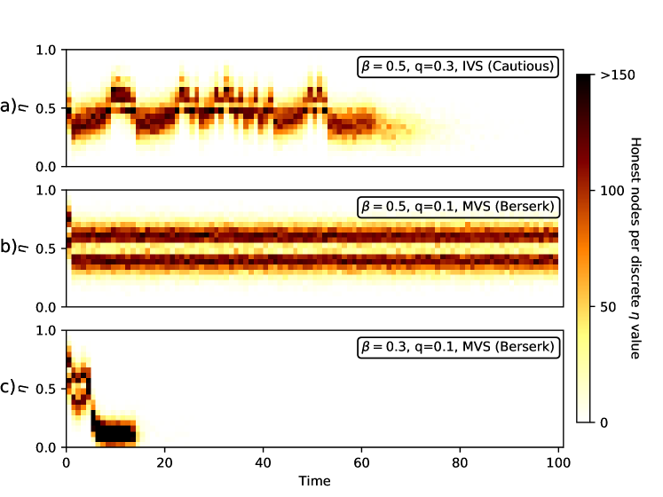
Figure 10: Evolution of the number of undecided nodes for a given $\eta$-value; [15].

Figures 12 and 12 show the variation of the termination and agreement rate with $q$ and $\beta$. The berserk attacker follows the MVS; and the network size is $n=1000$, $a=b=2/3$ and $\ell=10$. The maximal number of rounds is set to $100$. We consider the worst-case scenario ${\hat{p}}_{0}=a=b$. In cases where ${\hat{p}}_{0}$ differs from the initial threshold, the performances of FPC are significantly better. Recall that, if the protocol already starts in a “steep” part of the “potential” an attacker has practically no influence. It can be seen that if no randomness is employed the protocol can be prevented from terminating. Introducing randomness via decreasing $\beta$ improves the termination as well as the agreement rate. However, the figures also show that too much randomness can harm the performances.

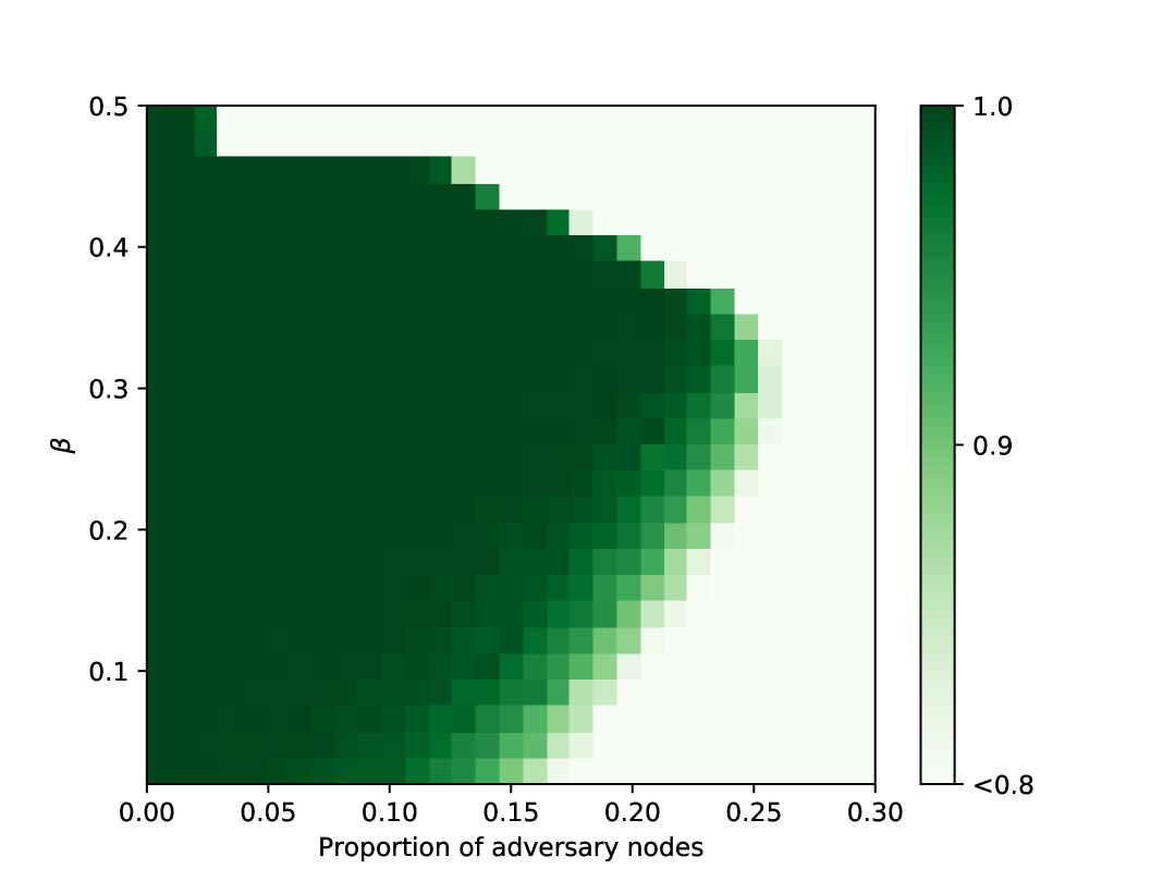
Figure 11: Termination rate; [15].

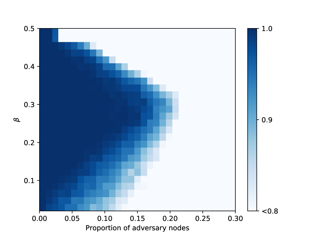
Figure 12: Agreement rate; [15].

3.5 Discussion

In the remaining part of this section, we discuss which assumptions are necessary for FPC.

Random thresholds

FPC relies in its construction on a (decentralized) random number generator that produces periodically random thresholds to break metastable situations. A first natural question is therefore how the robustness of FPC depends on the robustness of the random numbers. In fact, the answer is that FPC is rather robust towards failures of the external randomness. To see this, it is good to remind oneself of the functionality of the random threshold: it serves the consensus protocol to escape meta-stable states. For this purpose, it is sufficient that from time to time some sufficiently large proportion agrees on a random threshold. Let us make this more precise. We need that, regardless of the past, with probability at least $\theta$ (where $\theta>0$ is a fixed parameter) the next outcome is a uniform random variable which is unpredictable for the adversary. This random number is seen by at least $(1-\delta)$ proportion of honest nodes, where $\delta$ is reasonably small. What we can prove in such a situation depends on what the remaining $\delta(1-q)n$ honest nodes use as their decision thresholds: they can use some second candidate (in case there is an alternative source of common randomness), or they can choose their thresholds independently and randomly, etc. Each of such situations would need to be treated separately, which is certainly doable but left out of this paper. Let us note, though, that the worst-case assumption is that the adversary can “feed” the (fake) decision thresholds to those $\delta(1-q)n$ honest nodes. This would effectively mean that (at worst) these nodes would behave as cautious adversaries in the next round. This only matters if the random time $\Psi$ did not yet occur. Therefore, to obtain bounds like (21)–(23) and (22) we can simply pretend that the value of $q$ is increased by $\delta$.

Assuming that $\delta=0$, it is easy to figure out how this will affect our results: indeed, in our proofs, all random thresholds matter only until $\Psi$. We can obtain the following fact:

Proposition 3.3.

Assume the above on the random number generation (with $\theta\in(0,1)$ and $\delta=0$). Then, the estimates (21)–(23) and (22) remain valid (although, possibly, with other constants).

Also, we want to stress out that partial control of the random numbers does not give access to a lot of influence (in the worst-case the adversary would delay the consensus a bit). Hence, there is not much need to be restrictive on the degree of decentralization for that part: a smaller subcommittee can take care of the random numbers’ generation, and some VDF-based random number generation scheme (e.g., such as those of [44, 73]) may be used to further prevent this subcommittee from leaking the numbers before the due time.

We also refer to [15] for a numerical study of the FPC’s dependence on the “quality” of the random thresholds.

Complete network view

In the theoretical results of FPC, we assume that every node holds a complete network view. However, in permissionless systems or in less reliable networks with inevitable churns (nodes join and leave), this assumption is not necessarily verified. While churns can be modeled by faulty nodes, the situation of a partial view on the network participants deserves more attention. The property of whether two given nodes can know and query each other induces a natural network topology or underlying graph structure. This graph structure has a crucial impact on the performances of FPC (think about the extreme case where the diameter of the graph is large and the propagation of opinions may take a very long time). However, for situations where the graph is well connected, e.g., an expander graph, we believe that the theoretical results remain true and the proof strategy can be applied (however, with an increased technical difficulty). First numerical results in this direction were obtained in [52], where several graph topologies are modelled.

Sybil protection

The main security assumption on FPC is that an adversary is not supposed to control more than some given proportion (dependent on the threat model) of the total number of nodes. While in permissioned systems the total number of nodes can be controlled, the permissionless setting a priori allows an adversary to create an unlimited amount of identities; this is known as a so-called “Sybil” attack. Any real-world implementation of FPC in a permissionless system should therefore contain a Sybil protection. A natural generalization of FPC with a Sybil protection was given in [51, 52] and some mathematical properties were studied further in [38]. In this model, every node is given a certain weight (that may correspond to a scarce resource) or reputation. This weight is then used for choosing the queries and weighting the obtained opinions. We refer to [52] for more details on the protocol and security assumption in terms of percentages of weights instead of just proportions of the nodes.

In view of the above results, let us stress that one of the main features of FPC is that it turns “rather weak” consensus (on the random numbers, the participants of the network, and their weights) into a “strong” consensus on the value of a bit (i.e., the validity of a transaction), with high probability.

4 Conclusion

Majority dynamics are probably the most natural candidates for consensus protocols and promise scalable solutions for the DLT space. While protocols in this class behave well and their study is rather straightforward in an honest environment, the situation changes drastically in the presence of Byzantine actors. In particular, a possible attacker may keep the system in a so-called “metastable state” and prevent the honest nodes from finding consensus.

We suggested analyzing these protocols as random walks on a potential. This method offers a heuristic to understand the typical behavior and main issues of the standard majority dynamics. Finally, we gave an overview of the FPC protocol that uses common random thresholds to prevent the occurrence of metastable states and allows formal proofs of the security of the protocol.

References

- [1] Mohammed Amin Abdullah and Moez Draief. Global majority consensus by local majority polling on graphs of a given degree sequence. Discrete Applied Mathematics, 180:1 – 10, 2015.
- [2] Marcos K Aguilera and Sam Toueg. The correctness proof of Ben-Or’s randomized consensus algorithm. Distributed Computing, 25(5):371–381, 2012.
- [3] David J. Aldous. Markov chains with almost exponential hitting times. Stochastic Processes and their Applications, 13(3):305–310, 1982.
- [4] David J. Aldous and Mark Brown. Inequalities for rare events in time-reversible Markov chains. I, volume 22 of Lecture Notes–Monograph Series, pages 1–16. Institute of Mathematical Statistics, Hayward, CA, 1992.
- [5] David J. Aldous and Mark Brown. Inequalities for rare events in time-reversible Markov chains II. Stochastic Processes and their Applications, 44(1):15–25, 1993.
- [6] Yonatan Aumann and Yehuda Lindell. Security against covert adversaries: Efficient protocols for realistic adversaries. In Theory of Cryptography Conference, pages 137–156. Springer, 2007.
- [7] Luca Becchetti, Andrea Clementi, Emanuele Natale, Francesco Pasquale, and Luca Trevisan. Stabilizing consensus with many opinions. In Proceedings of the twenty-seventh annual ACM-SIAM symposium on Discrete algorithms, pages 620–635. SIAM, 2016.
- [8] M. Belotti, N. Božić, G. Pujolle, and S. Secci. A vademecum on blockchain technologies: When, which, and how. IEEE Communications Surveys Tutorials, 21(4):3796–3838, 2019.
- [9] Michael Ben-Or. Another advantage of free choice: Completely asynchronous agreement protocols (extended abstract). In Proceedings of the 2nd ACM Annual Symposium on Principles of Distributed Computing, Montreal, Quebec, pages 27–30, 1983.
- [10] Itai Benjamini, Siu-On Chan, Ryan O’Donnell, Omer Tamuz, and Li-Yang Tan. Convergence, unanimity and disagreement in majority dynamics on unimodular graphs and random graphs. Stochastic Processes and their Applications, 126(9):2719 – 2733, 2016.
- [11] Anton Bovier and Frank den Hollander. Metastability. A potential-theoretic approach. Springer, 2016.
- [12] Anton Bovier, Michael Eckhoff, Véronique Gayrard, and Markus Klein. Metastability in reversible diffusion processes I: Sharp asymptotics for capacities and exit times. Journal of European Mathematical Society, 6:399–424, 2004.
- [13] Gabriel Bracha. Asynchronous Byzantine agreement protocols. Information and Computation, 75(2):130–143, 1987.
- [14] Maury Bramson, J.Theodore Cox, and Jean-François Le Gall. Super-Brownian limits of voter model clusters. Ann. Probab., 29(3):1001–1032, 07 2001.
- [15] Angelo Capossele, Sebastian Mueller, and Andreas Penzkofer. Robustness and efficiency of leaderless probabilistic consensus protocols within Byzantine infrastructures, 2019.
- [16] Ignacio Cascudo and Bernardo David. Scrape: Scalable randomness attested by public entities. In International Conference on Applied Cryptography and Network Security, pages 537–556. Springer, 2017.
- [17] Marzio Cassandro, Antonio Galves, Enzo Olivieri, and Maria Eulália Vares. Metastable behavior of stochastic dynamics: A pathwise approach. Journal of Statistical Physics, 35(5-6):603–634, June 1984.
- [18] Peter Clifford and Aidan Sudbury. A model for spatial conflict. Biometrika, 60(3):581–588, 1973.
- [19] Edgar F. Codd. Cellular Automata. Academic Press, 1968.
- [20] F. Comets and S. Popov. Limit law for transition probabilities and moderate deviations for Sinai’s random walk in random environment. Probab. Theory Related Fields, 126(4):571–609, 2003.
- [21] Colin Cooper, Robert Elsässer, and Tomasz Radzik. The power of two choices in distributed voting. In International Colloquium on Automata, Languages, and Programming, pages 435–446. Springer, 2014.
- [22] Colin Cooper, Robert Elsässer, Tomasz Radzik, Nicolas Rivera, and Takeharu Shiraga. Fast consensus for voting on general expander graphs. In International Symposium on Distributed Computing, pages 248–262. Springer, 2015.
- [23] J. Theodore Cox, Richard Durrett, and Edwin A. Perkins. Rescaled voter models converge to super-Brownian motion. Ann. Probab., 28(1):185–234, 01 2000.
- [24] J. Theodore Cox and David Griffeath. Occupation time limit theorems for the voter model. Ann. Probab., 11(4):876–893, 11 1983.
- [25] James Cruise and Ayalvadi Ganesh. Probabilistic consensus via polling and majority rules. Queueing Syst. Theory Appl., 78(2):99–120, October 2014.
- [26] Amir Dembo, Alice Guionnet, and Ofer Zeitouni. Aging properties of Sinai’s model of random walk in random environment. In St. Flour Summer School 2001, Springer’s Lecture Notes in Mathematics, volume 1837, 2001.
- [27] Benjamin Doerr, Leslie Ann Goldberg, Lorenz Minder, Thomas Sauerwald, and Christian Scheideler. Stabilizing consensus with the power of two choices. In Proceedings of the Twenty-Third Annual ACM Symposium on Parallelism in Algorithms and Architectures, SPAA ’11, page 149–158, New York, NY, USA, 2011. Association for Computing Machinery.
- [28] R. Durrett. Probability: theory and examples. Cambridge Series in Statistical and Probabilistic Mathematics. Cambridge University Press, Cambridge, fourth edition, 2010.
- [29] Robert Elsässer, Tom Friedetzky, Dominik Kaaser, Frederik Mallmann-Trenn, and Horst Trinker. Rapid asynchronous plurality consensus. arXiv preprint arXiv:1602.04667, 2016.
- [30] Nathanaël Enriquez, Christophe Sabot, and Olivier Zindy. Aging and quenched localization for one-dimensional random walks in random environment in the sub-ballistic regime. Bulletin de la Société Mathématique de France, 137(3):423–452, 2009.
- [31] Giulia Fanti, Nina Holden, Yuval Peres, and Gireeja Ranade. Communication cost of consensus for nodes with limited memory. Proceedings of the National Academy of Sciences, 117(11):5624–5630, 2020.
- [32] Paul Feldman and Silvio Micali. An optimal probabilistic algorithm for synchronous Byzantine agreement. In International Colloquium on Automata, Languages, and Programming, pages 341–378. Springer, 1989.
- [33] M.I. Freidlin, J. Szücs, and A.D. Wentzell. Random Perturbations of Dynamical Systems. Grundlehren der mathematischen Wissenschaften. Springer, 2012.
- [34] Roy Friedman, Achour Mostefaoui, and Michel Raynal. Simple and efficient oracle-based consensus protocols for asynchronous Byzantine systems. IEEE Transactions on Dependable and Secure Computing, 2(1):46–56, 2005.
- [35] P. Gács, G. L. Kurdyumov, and Leonid A. Levin. One-dimensional uniform arrays that wash out finite islands. In Problemy Peredachi Informatsii, 1978.
- [36] Bernd Gärtner and Ahad N. Zehmakan. Majority model on random regular graphs. Lecture Notes in Computer Science, pages 572–583, 2018.
- [37] Alexander Gogolev, Nikolaj Marchenko, Lucio Marcenaro, and Christian Bettstetter. Distributed binary consensus in networks with disturbances. ACM Trans. Auton. Adapt. Syst., 10(3):19:1–19:17, September 2015.
- [38] A. Gutierrez, S. Müller, and S. Šebek. On asymptotic fairness in voting consensus protocols. 2021.
- [39] Richard A. Holley and Thomas M. Liggett. Ergodic theorems for weakly interacting infinite systems and the voter model. The Annals of Probability, 3(4):643–663, 1975.
- [40] Arkadiusz Jedrzejewski and Katarzyna Sznajd-Weron. Statistical physics of opinion formation: Is it a spoof? Comptes Rendus Physique, 20(4):244–261, 2019.
- [41] S. Kar and J. M. F. Moura. Distributed average consensus in sensor networks with random link failures. In 2007 IEEE International Conference on Acoustics, Speech and Signal Processing - ICASSP ’07, volume 2, pages II–1013–II–1016, April 2007.
- [42] Julian Keilson. Markov chain models – rarity and exponentiality. Applied Mathematical Sciences 28. Berlin-Heidelberg-New York, Springer-Verlag 1979. ZAMM - Journal of Applied Mathematics and Mechanics / Zeitschrift für Angewandte Mathematik und Mechanik, 60(5):272–272, 1980.
- [43] Thomas G. Kurtz and Jason Swanson. Finite Markov chains coupled to general Markov processes and an application to metastability I, 2021.
- [44] Arjen K. Lenstra and Benjamin Wesolowski. Trustworthy public randomness with sloth, unicorn, and trx. International Journal of Applied Cryptography, 3(4):330–343, 2017.
- [45] Thomas M. Liggett. Interacting particle systems, volume 276. Springer Science & Business Media, 2012.
- [46] Francesco Manzo, Matteo Quattropani, and Elisabetta Scoppola. A probabilistic proof of Cooper and Frieze’s ”First Visit Time Lemma”, 2021.
- [47] Francesco Manzo and Elisabetta Scoppola. Exact results on the first hitting via conditional strong quasi-stationary times and applications to metastability. Journal of Statistical Physics, 174:1239–1262, 2019.
- [48] Mikhail Menshikov, Serguei Popov, and Andrew Wade. Non-homogeneous random walks – Lyapunov function methods for near-critical stochastic systems. Cambridge University Press, Cambridge, 2017.
- [49] A.A. Moreira, A. Mathur, D. Diermeier, and L.A.N. Amaral. Efficient system-wide coordination in noisy environments. Proc. Natl. Acad. Sci. U.S.A., 101:12085–12090, AUG 2004.
- [50] Elchanan Mossel, Joe Neeman, and Omer Tamuz. Majority dynamics and aggregation of information in social networks. Autonomous Agents and Multi-Agent Systems, 28(3):408–429, Jun 2013.
- [51] S. Müller, A. Penzkofer, D. Camargo, and O. Saa. On fairness in voting consensus protocols. Computing Conference 21, to appear.
- [52] Sebastian Müller, Andreas Penzkofer, Bartosz Kuśmierz, Darcy Camargo, and William J. Buchanan. Fast Probabilistic Consensus with weighted votes. FTC 2020. Advances in Intelligent Systems and Computing, vol 1289, 2, 2020.
- [53] Satoshi Nakomoto. Bitcoin: A Peer-to-Peer Electronic Cash System. https://bitcoin.org/bitcoin.pdf, 2008.
- [54] NKN Lab. NKN: a scalable self-evolving and self-incentivized decentralized network, 2018.
- [55] Piotr Nyczka, Jerzy Cisło, and Katarzyna Sznajd-Weron. Opinion dynamics as a movement in a bistable potential. Physica A: Statistical Mechanics and its Applications, 391(1):317–327, 2012.
- [56] Enzo Olivieri and Maria Eulália Vares. Large Deviations and Metastability. Encyclopedia of Mathematics and its Applications. Cambridge University Press, 2005.
- [57] O. Penrose and J. L. Lebowitz. Rigorous treatment of metastable states in the van der Waals-Maxwell theory. Journal of Statistical Physics, 3(2):211–236, June 1971.
- [58] Serguei Popov. On a decentralized trustless pseudo-random number generation algorithm. Journal of Mathematical Cryptology, 11(1):37–43, 2017.
- [59] Serguei Popov. Two-Dimensional Random Walk – From Path Counting to Random Interlacements. Cambridge University Press, 2021.
- [60] Serguei Popov and William J. Buchanan. FPC-BI: Fast Probabilistic Consensus within Byzantine Infrastructures. Journal of Parallel and Distributed Computing, 147:77–86, 2021.
- [61] Errico Presutti and Herbert Spohn. Hydrodynamics of the voter model. Ann. Probab., 11(4):867–875, 11 1983.
- [62] Michael O Rabin. Randomized Byzantine generals. In 24th Annual Symposium on Foundations of Computer Science (sfcs 1983), pages 403–409. IEEE, 1983.
- [63] Sidney Redner. Reality-inspired voter models: A mini-review. Comptes Rendus Physique, 20(4):275–292, 2019.
- [64] Team Rocket. Snowflake to Avalanche: A novel metastable consensus protocol family for cryptocurrencies, 2018.
- [65] Team Rocket, Maofan Yin, Kevin Sekniqi, Robbert van Renesse, and Emin Gün Sirer. Scalable and probabilistic leaderless BFT consensus through metastability, 2019.
- [66] Sheldon M. Ross. Introduction to Probability Models. Academic Press, 10th edition, 2009.
- [67] Philipp Schindler, Aljosha Judmayer, Nicholas Stifter, and Edgar Weippl. Hydrand: Practical continuous distributed randomness. Cryptology ePrint Archive, Report 2018/319, 2018. https://eprint.iacr.org/2018/319.
- [68] Ya.G. Sinaj. Limit behavior of the one-dimensional random walks in random environments. Teor. Veroyatn. Primen., 27:247–258, 1982.
- [69] Richard B. Sowers. Hydrodynamical limits and geometric measure theory: Mean curvature limits from a threshold voter model. Journal of Functional Analysis, 169(2):421–455, 1999.
- [70] Ewa Syta, Philipp Jovanovic, Eleftherios Kokoris Kogias, Nicolas Gailly, Linus Gasser, Ismail Khoffi, Michael J Fischer, and Bryan Ford. Scalable bias-resistant distributed randomness. In 2017 IEEE Symposium on Security and Privacy (SP), pages 444–460. IEEE, 2017.
- [71] Mieko Tanaka-Yamawaki, Sachiko Kitamikado, and Toshio Fukuda. Consensus formation and the cellular automata. Robotics and Autonomous Systems, 19(1):15–22, 1996.
- [72] Linh V. Tran and Van Vu. Reaching a consensus on random networks: The power of few. In Jaroslaw Byrka and Raghu Meka, editors, Approximation, Randomization, and Combinatorial Optimization. Algorithms and Techniques, APPROX/RANDOM 2020, August 17-19, 2020, Virtual Conference, volume 176 of LIPIcs, pages 20:1–20:15. Schloss Dagstuhl - Leibniz-Zentrum für Informatik, 2020.
- [73] Benjamin Wesolowski. Efficient verifiable delay functions. J. Cryptol., 33:2113–2147, 2020.
- [74] Stephen Wolfram. Cellular Automata and Complexity: Collected Papers. Westview Press, 1994.