HSMA: An $O(N)$ electrostatics package implemented in LAMMPS

Abstract

We implement two recently developed fast Coulomb solvers, HSMA3D [J. Chem. Phys. 149 (8) (2018) 084111] and HSMA2D [J. Chem. Phys. 152 (13) (2020) 134109], into a new user package HSMA for molecular dynamics simulation engine LAMMPS. The HSMA package is designed for efficient and accurate modeling of electrostatic interactions in 3D and 2D periodic systems with dielectric effects at the $O(N)$ cost. The implementation is hybrid MPI and OpenMP parallelized and compatible with existing LAMMPS functionalities. The vectorization technique following AVX512 instructions is adopted for acceleration. To establish the validity of our implementation, we have presented extensive comparisons to the widely used particle-particle particle-mesh (PPPM) algorithm in LAMMPS and other dielectric solvers. With the proper choice of algorithm parameters and parallelization setup, the package enables calculations of electrostatic interactions that outperform the standard PPPM in speed for a wide range of particle numbers.

PROGRAM SUMMARY/NEW VERSION PROGRAM SUMMARY

Program Title: HSMA
CPC Library link to program files: (to be added by Technical Editor)
Developer’s repository link:https://github.com/LiangJiuyang/HSMA-Harmonic-surface-mapping-algorithm-in-LAMMPS
Code Ocean capsule: (to be added by Technical Editor)
Licensing provisions(please choose one): GPLv3
Programming language: C++
Nature of problem: Evaluation of long-range electrostatic interactions for charged system with fully periodic condition or confined by planar dielectric interfaces.
Solution method: We implement the Harmonic Surface Mapping algorithm (HSMA), which combines the image-charge method with the harmonic surface mapping and converts the contribution of infinite images into a finite number of surface charges on an auxiliary sphere, into simulation package LAMMPS. The HSMA package works for both fully periodic system and partially periodic system with planar dielectric interfaces, achieving truly linear $O(N)$ complexity by employing fast multiple method. Our package can be applied to general all-atom simulation and a broad range of charged complex fluids under dielectric confinement.
Additional comments: Hybrid MPI plus OpenMP parallelization is used in HSMA package for high-performance computing. We provide vertor optimization by using the AVX512 instructions and Intel MKL library for further acceleration. Intel parallel studio is required for these techniques.

1 Introduction

Electrostatic interactions play a key role in nanoparticle self-assembly processes [1, 2], and are also so ubiquitous in biomolecular systems, such as DNA aggregation [3] and polyelectrolyte complexation [4, 5, 6]. Numerical simulations, such as Monte Carlo (MC) and molecular dynamics (MD), provide higher accuracy for understanding the long-range nature of the Coulomb interactions, compared to theoretical efforts at the mean-field level [7, 8]. In computer simulations, periodic boundary conditions (PBCs) are often employed for approximating an infinite system by using a small unit cell [9]. To efficiently sum over the contribution of charges in the infinite periodic replicates, the common approaches rely on the conventional Ewald summation [scaling with the particle number $N$ as $O(N^{3/2})$] [10] and its variations such as particle-particle particle-mesh Ewald (PPPM) [scaling $O(N\log(N))$] [11] and random batch Ewald (RBE) [scaling $O(N)$] [12], or the multipole-type methods such as the tree code [scaling $O(N\log(N))$] [13] and the fast multipole method (FMM) [scaling $O(N)$] [14]. Given their prevalence, the efficient parallel implementations [15, 16, 17] in MD simulation packages such as LAMMPS [18] and GROMACS [19] and the comparisons of these methods [20] have been the subject of considerable computational research efforts.

Furthermore, many materials interfaces are characterized by a discontinuity in the permittivity, resulting in induced surface polarization charges. This induced charge may significantly affect the ionic distributions [21, 22, 23, 24, 25, 26] and dynamics [27, 28, 29], so that developing efficient methods for modeling spatially varying dielectrics has received considerable research attention [30, 31, 32, 33, 34, 35, 36]. Whereas this is typically costly, the special situation of planar interfaces (as well as systems that can be approximated as such) can be treated highly efficiently and accurately via the well-known image-charge method (ICM) [37]. Still, in the presence of two planar interfaces, this leads to iterative image reflections, so that the summation over the infinite image charges is a non-trivial task and several numerical methods such as ICM-MMM2D [38] (scaling $\mathcal{O}(N^{5/3})$), ectrostatic layer correction method [39] (ICM-ELC, scaling as $\mathcal{O}(N\log N)$), ICM-Ewald [40] (scaling as $\mathcal{O}(N^{3/2})$), and ICM-PPPM (scaling as $\mathcal{O}(N\log(N))$) [41] have been proposed.

To benefit the community, we present a parallel implementation of two previously formulated HSMA methods [42, 43] into the popular MD package LAMMPS [44], producing highly efficient solvers for modeling electrostatic interactions in 3D and 2D periodic system. This article describes the new implementation and analyses its performance. The organization of this article is as follows. In Section 2, we present a description of the simulation model, with a brief review of our HSMA algorithms. Section 3 provides the details of the LAMMPS implementation. In Section 4, we apply the method to three types of charged systems and confirm the correct implementation in LAMMPS: primitive electrolytes and SPC/E water in 3D bulk, and primitive electrolytes confined between parallel dielectric interfaces. In Section 5, we analyze the CPU performance of the HSMA.

2 Overview of simulation model and HSMA

2.1 Simulation model

The package is designed for modeling two types of systems, namely 3D-periodic system and 2D-periodic system with dielectric boundaries.

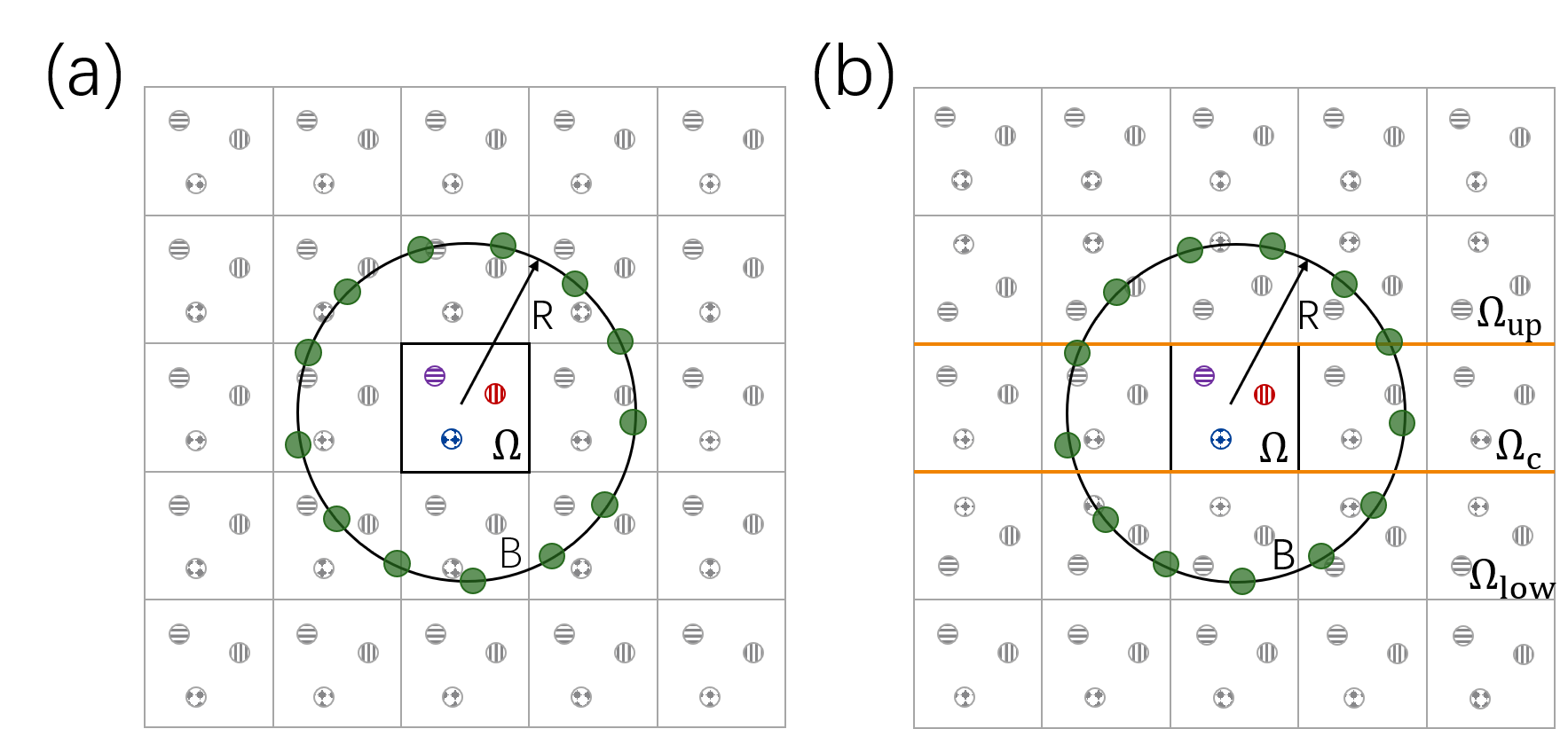
Figure 1: Schematic illustration of the HSMA3D (a) and HSMA2D (b) for an infinite ionic system under fully/partially periodic system. $\Omega$ is the central box, and particles within it are the sources. Polarization is approximated by the sum of contributions from image charges inside the spherical boundary $\partial B$ and the finite point charges (green sphere) on $\partial B$. The orange lines indicate the locations of dielectric interface.

A set of $N$ point charges located at positions $\{\bm{r}_{i}=(x_{i},y_{i},z_{i}),~{}i=1,\cdots,N\}$ with strengths $\{q_{i},~{}i=1,\cdots,N\}$ is placed in the central cuboidal box $\Omega=[-L_{x}/2,L_{x}/2]\times[-L_{y}/2,L_{y}/2]\times[-L_{z}/2,L_{z}/2]$ which is characterized by a dielectric constant $\varepsilon_{\text{c}}$. For 3D-periodic case, the central simulation box is copied along $x$-, $y$-, and $z$-dimensions, resulting in an infinite number of periodic copies [Fig. 1(a)]. In a 2D-periodic system, the simulation box is replicated along $x$- and $y$-dimensions where the particles are confined by two dielectric boundaries at $z=\pm L_{z}/2$. These interfaces separate the entire space $\mathcal{R}$ into three layers which are labeled $\Omega_{\text{up}}$, $\Omega_{\text{c}}$, and $\Omega_{\text{low}}$ with dielectric constant $\varepsilon_{\text{up}}$, $\varepsilon_{\text{c}}$, and $\varepsilon_{\text{low}}$, respectively [Fig. 1(a)].

Let $\Phi(r)$ be the electrostatic potential that satisfies the Poisson’s equation within $\Omega$,

$$-\nabla\cdot\varepsilon(\bm{r})\nabla\Phi(\bm{r})=4\pi\sum_{j=1}^{N}q_{j}\delta(\bm{r}-\bm{r}_{j}),$$ (1)

where $\delta(\bm{r})$ is the Dirac function and the solution can be expressed as an infinite sum,

$$\varepsilon_{\text{c}}\Phi(\bm{r})=\sum_{j=1}^{N}\dfrac{q_{j}}{|\bm{r}_{j}-\bm{r}|}+\sum_{j=N+1}^{\infty}\dfrac{q_{j}}{|\bm{r}_{j}-\bm{r}|},$$ (2)

where the first term is the direct potential from the source charges and the second term describes the contribution of infinite images which are introduced to satisfy the boundary conditions. If the system is fully periodic, we have

$$\varepsilon_{\text{c}}\Phi(\bm{r})=\sum_{\bm{k}}\sum_{j=1}^{N}\dfrac{q_{j}}{|\bm{r}_{j}+\bm{k}\circ\bm{L}-\bm{r}|},$$ (3)

where $\bm{k}=(k_{x},k_{y},k_{z})$ runs over all three-dimensional integer vectors and $\bm{L}=(L_{x},L_{y},L_{z})$. Here $\circ$ indicates the element-wise multiplication. For a 2D-periodic system with dielectric boundaries, the solution $\Phi_{\text{c}}(\bm{r})$ within $\Omega_{\text{c}}$ can be conveniently expressed using the image charge construction, leading to,

$$\begin{split}\varepsilon_{\text{c}}\Phi_{\text{c}}(\bm{r})=&\sum_{\bm{k}}\sum_{i=1}^{N}\dfrac{q_{i}}{|\bm{r}_{i}+\bm{k}\circ\bm{L}-\bm{r}|}\\ &+\sum_{\bm{k}}\sum_{i=1}^{N}\sum_{\ell=1}^{\infty}\left(\dfrac{q_{i}\gamma_{\ell}^{+}}{|\bm{r}_{i+}^{(\ell)}+\bm{k}\circ\bm{L}-\bm{r}|}+\dfrac{q_{i}\gamma_{\ell}^{-}}{|\bm{r}_{i-}^{(\ell)}+\bm{k}\circ\bm{L}-\bm{r}|}\right),\end{split}$$ (4)

where $\bm{k}=(k_{x},k_{y},0)$ represents all two-dimensional integer vectors, $\gamma_{\text{up}}=(\varepsilon_{\text{c}}-\varepsilon_{\text{up}})/(\varepsilon_{\text{c}}+\varepsilon_{\text{up}})$ and $\gamma_{\text{low}}=(\varepsilon_{\text{c}}-\varepsilon_{\text{low}})/(\varepsilon_{\text{c}}+\varepsilon_{\text{low}})$ are dielectric mismatches, $\gamma_{\ell}^{+}=\gamma_{\text{low}}^{\lceil\ell/2\rceil}\gamma_{\text{up}}^{\lfloor\ell/2\rfloor}$, $\gamma_{\ell}^{-}=\gamma_{\text{low}}^{\lfloor\ell/2\rfloor}\gamma_{\text{up}}^{\lceil\ell/2\rceil}$, and the position $\bm{r}_{i\pm}^{(\ell)}$ of the $\ell$th-order image of charge $q_{i}$ is $\bm{r}_{i\pm}^{(\ell)}=(x_{i},y_{i},(-1)^{\ell}z_{i}\pm\ell L_{z})$. Here +(-) corresponds to the image charges in $\Omega_{\text{up}}$($\Omega_{\text{low}}$) and the notation $\lceil x\rceil$($\lfloor x\rfloor$) represents the ceil (floor) function.

2.2 Review of HSMA algorithms

The HSMA algorithms for 3D and 2D periodic systems were described in detail in Refs. [42] and [43], respectively. Here we give a brief overview of the most important features of the algorithm. A flow chart of the HSMA algorithms is presented in Fig. 2.

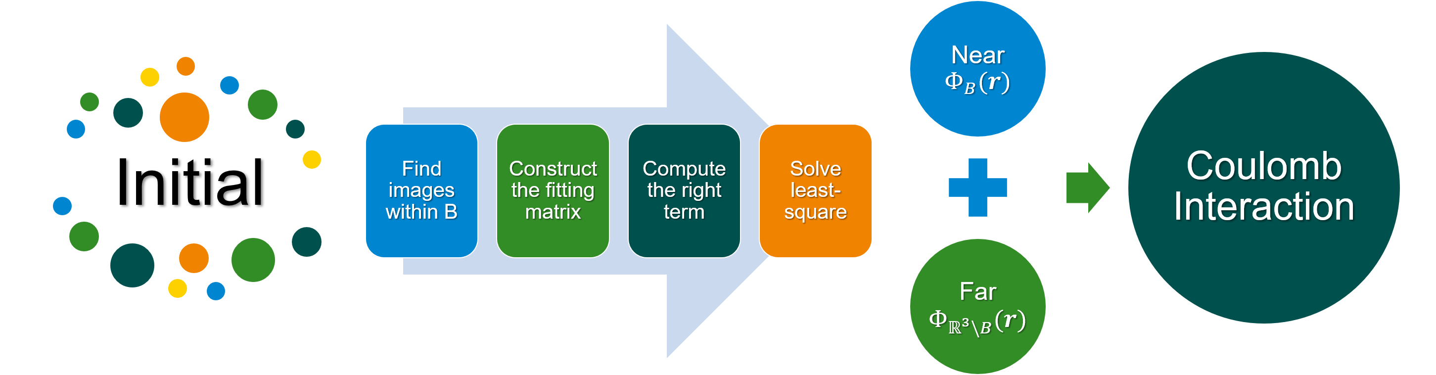
Figure 2: The flow chart of the HSMA algorithm.

First, we find all the images of the source charges within the auxiliary sphere $B$, which includes both periodic images and image charges that are introduced to satisfy dielectric boundary conditions. We define $\{q_{s},~{}s=1,\cdots,N_{s}\}$ to be the set of sources and corresponding image charges within the sphere. Since the electrostatic potential $\Phi_{\mathbb{R}^{3}\backslash B}(\bm{r})$ of charges outside the sphere $B$ is a harmonic function in the domain $\Omega$, the potential $\Phi(\bm{r})$ can be split into two parts,

$$\Phi(\bm{r})=\Phi_{B}(\bm{r})+\Phi_{\mathbb{R}^{3}\backslash B}(\bm{r})=\sum_{j=1}^{N_{s}}\dfrac{q_{j}}{|\bm{r}_{j}-\bm{r}|}+\sum_{n=0}^{P}\sum_{m=-n}^{n}A_{n}^{m}r^{n}Y_{n}^{m}(\vartheta,\varphi)\;,$$ (5)

where $\Phi_{\mathbb{R}^{3}\backslash B}(\bm{r})$ is approximated by a truncated spherical harmonic series [45] with the total number of spherical basis $N_{b}=(P+1)^{2}$, $Y_{n}^{m}$ is the spherical harmonic function of degree $n$ and order $m$, $\{A_{n}^{m},~{}n=0,\cdots,P,~{}m=-n,\cdots,n\}$ is a set of unknown coefficients.

Second, we determine the coefficients $A_{n}^{m}$ of the truncated spherical harmonic series [Eq. (5)] by constructing the fitting matrix and computing the right vector. In the case of a 3D periodic system, we generate $N_{m}$ ($>N_{b}$) monitoring points which are nearly uniformly distributed on the circumsphere $B$ of the central cell $\Omega$. The coefficients ${A_{n}^{m}}$ are obtained by solving the least square problem at these points [42],

$${A_{n}^{m}}=\text{argmin}\sum_{i=1}^{N_{m}}|\mathcal{L}(\Phi(\bm{r}_{i}))|^{2}=\text{argmin}\|MA-Y\|_{L^{2}},$$ (6)

where $\mathcal{L}$ is a linear operator on $A_{n}^{m}$, $A$ represents the vector consisting of all the elements of $A_{n}^{m}$, $Y$ is the right vector which depends on the $\Phi_{B}(\bm{r})$ of monitoring points, and $M$ is the mapping matrix which depends on the locations of monitoring points and the degrees and orders of spherical basis and can be constructed in the preparation step. For a 2D periodic system with dielectric boundary conditions, the above minimization step cannot be efficiently applied since the dielectric conditions require information about the exterior domain of the simulation box $\Omega$. To overcome this issue, we introduce the Dirichlet-to-Neumann (DtN) boundary condition in Ref. [43], which transforms the dielectric conditions into a surface integral that only requires knowledge of $\Phi_{\text{c}}$ and its derivative in $z$-direction. The coefficients $A_{n}^{m}$ are then obtained by minimizing the residual norm of the DtN boundary condition which is approximated via the $2$D-dilation formula [46].

Third, we map the spherical harmonic expansion onto a surface integral over the sphere $B$, which is the core idea of HSMA and permits the use of the FMM. The main advantages is that such a step avoids the repeated evaluation of spherical harmonic basis through the recursive relations due to its less efficient especially for parallel computation. The surface charge integral is not singular and can be approximated by common numerical quadratures such as Fibonacci integration which has a convergence rate of $N_{o}^{-6}$ with $N_{o}$ the number of grid points.

Finally, the FMM can be easily employed to sum over all charges within and on the sphere, achieving a truly linear $O(N)$ complexity. However, direct summation with $O(N^{2})$ complexity is also implemented in our package.

3 LAMMPS implementation of HSMA

3.1 Implementation details

The software is open-source and distributed under GNU General Public License (GPL). We implement the HSMA methods described above into LAMMPS as an optional package called USER-HSMA, providing two new kspace solvers with $O(N)$ complexity for charged systems with 3D and 2D periodicity. The code is available for download from the author’s Github page (https://github.com/LiangJiuyang), including documentation and examples. The software can be installed via make yes-user-hsma or by directly copying the files into the LAMMPS main source directory and compiling the code. The required dependent package is the Intel Parallel Studio [47] (including functions of MPI, OpenMP, MKL library, and AVX512 instructions).

The two new kspace styles are called HSMA3D and HSMA2D, which treats the long-range electrostatic interactions of 3D periodic system and 2D periodic system with dielectric interfaces, respectively. The function of HSMA3D is the same as the classical Ewald and the PPPM in LAMMPS, whereas HSMA3D has the most optimal $O(N)$ complexity by the use of the FMM. Furthermore, no alternative approaches for 2D periodic system with dielectric interfaces have been implemented into LAMMPS, and we believe the implementation of HSMA2D will greatly benefit the general computational physics community. Both solvers allow large scale simulations of molecular systems and are very general as they can be easily combined with other bonded and non-bonded interactions.

The current workflow of our codes is shown in Fig. 3. The interfaces of the information of systems and the MPI ranks are accessed within the constructor. The “Settings” function includes the computation before the first timestep of a run, including reading parameters and allocating storages. The “Init” function initializes the calculation before a run, including the generation of the Fibonacci quadratures, the monitoring points, and the 2D-dilation quadratures. The “Compute” function, which executes at every time step, involves a complete algorithm flow.

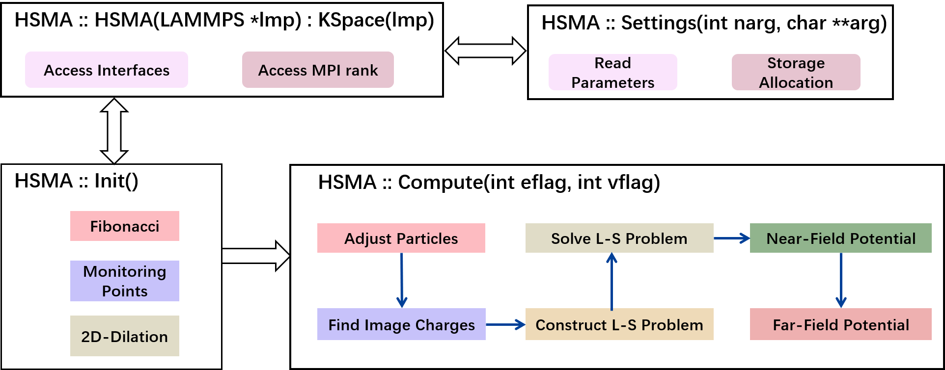
Figure 3: The implemented CPU workflow of our HSMA codes in LAMMPS.

Our current implementation supports massively parallel MD simulation of large-scale particle systems. We use Intel’s 512-bit SIMD (AVX-512 architecture) for vectorization implementation outline in which eight neighbors for double precision (or sixteen for float) are operated at the same time, and hybrid MPI plus OpenMP are employed for parallelization. Although the compiler can automatically vectorize loops, it is sometimes necessary to make changes to the codes which can improve vectorization efficiency. The pure MPI parallelization is permitted, but we suggest one use few MPI nodes but more OpenMP threads of each MPI, because of the saving of communication cost. Our implementation is consistent with the existing parallelization options provided in LAMMPS.

The interfaces of positions, forces, strengths, and other required MD parameters are obtained from the current class. After execution, the electrostatic energy, the force of atoms, and the potential are appended to the thermodynamic output which is useful because one can directly obtain the required results for different systems without any further changing in the input file or the source codes, except the kspace_style command.

3.2 Setup in LAMMPS

We describe the practical usage of HSMA3D and HSMA2D in LAMMPS. The methods can be readily invoked by setting the following command lines in LAMMPS,

kspace_style HSMA3D $\varepsilon_{\text{tol}}$ $\lambda$ $P$ $N_{m}$ $F_{w}$ $F$ $f_{1}$ $f_{2}$
kspace_style HSMA2D $\varepsilon_{\text{tol}}$ $\lambda$ $\gamma$ $P$ $N_{w}$ $W$ $F_{w}$ $F$ $f_{1}$ $f_{2}$

where the former works for fully periodic systems and the latter works for partially periodic systems.

The HSMA3D style invokes the HSMA algorithm for 3D periodic system [42]. The specified parameter $\varepsilon_{\text{tol}}$ is a double-precision variable that ranges from $0$ (exclude $0$) to $1$. This parameter will take effect on the accuracy of the FMM. If one chooses direct summation instead of the FMM, the float64 vector is used for vectorization when $\varepsilon_{\text{tol}}<10^{-6}$; otherwise, when $\varepsilon_{\text{tol}}\geq 10^{-6}$, the float32 vector is performed. The parameter $\lambda$ is a double-precision variable (larger than $1$) that represents the relative ratio of the radius of the auxiliary surface and the diagonal length of the simulation box. A larger $\lambda$ means that more images are included within the auxiliary surface, thus increases the cost but improves the accuracy. The parameter $P$ is a positive integer which indicates that the total number of spherical basis is $(P+1)^{2}$. The parameter  $N_{m}$ is the number of monitoring points $N_{m}$ which should be larger than $(P+1)^{2}$. A recommended choice is that $N_{m}=2(P+1)^{2}$. The parameters $F_{w}$ and $F$ are two adjacent integers in the Fibonacci sequence used in spherical integration. In most cases, $F_{w}=55$ and $F=89$ are accurate enough. The parameters $f_{1}$ and $f_{2}$ are integers that are either $1$ or $0$, indicating whether using the FMM or not when calculating the potential at the monitoring points and the near-field potential at the source points.

The HSMA2D style invokes the HSMA algorithm for 2D periodic system with dielectric interfaces [43]. The definitions of $\lambda$, $P$, $F_{w}$, $F$, $f_{1}$, and $f_{2}$ are the same as in the HSMA3D style. Three additional parameters are specified: the parameter $\gamma\in[-1,1]$ is the dielectric mismatch, and $N_{w}$ and $W$ are two integers used in the 2D-dilation formula with the total number of quadratures along $X$ and $Y$ dimensions as $N_{w}\lfloor\sqrt{W}\rfloor$.

The algorithm parameters used to attain different accuracies can be found in Refs. [42, 43, 48]. For an electrostatic accuracy of $10^{-5}$ which is often adopted for practical simulations, we can safely set

kspace_style HSMA3D $\varepsilon_{\text{tol}}$ $1.3$ $10$ $200$ $55$ $89$ $1$ $0$
kspace_style HSMA2D $\varepsilon_{\text{tol}}$ $1.6$ $0.94$ $6$ $40$ $4$ $55$ $89$ $0$ $1$

The package requires the use of a matching pair style to perform short-range pairwise calculations, for example “lj/cut/omp” is recommended for a primitive model electrolyte where particles interact via both long-range Coulomb interactions and short-range Lennard-Jones (LJ) interactions. That said, one should not not use any style which contains “coul/long” since the solvers HSMA3D and HSMA2D already contain fully electrostatic interactions.

4 Accuracy benchmark

4.1 Primitive monovalent, divalent, and trivalent electrolytes

To confirm the correct functioning of HSMA3D in our package, we study primitive electrolytes in a 3D periodic system. All ions are modeled as soft spheres of diameter $\sigma$ that interact through purely repulsive shifted-truncated LJ potential with energy coupling $\varepsilon_{\text{LJ}}=k_{\text{B}}T$, where $k_{\text{B}}$ is the Boltzmann constant and $T$ is the absolute temperature. The system has dimensions $L_{x}=25\sigma$, $L_{y}=25\sigma$, and $L_{z}=25\sigma$. We consider three types of model electrolytes, namely monovalent, divalent, and trivalent electrolytes containing $1500$, $1000$, $750$ cations and $1500$, $2000$, $2250$ anions, respectively, resulting in a volume fraction $10.05\%$. The ions are immersed in continuum solvent characterized by a Bjerrum length $\ell_{\text{B}}=e^{2}/(4\pi\varepsilon_{\text{c}}k_{\text{B}}T)=3.5\sigma$. We utilize a time step of $0.01\tau$, where $\tau=\sigma\sqrt{m_{0}/k_{\text{B}}T}$ is the unit of time with $m_{0}=1$ (LJ unit) the ion mass. The simulations are performed in the canonical ensemble, where the temperature is controlled by a Nos$\acute{\text{e}}$-Hoover thermostat with damping time $0.01\tau$. Energy minimization proceeds for $2\times 10^{5}$ time steps, followed by a production period which occupies $10^{7}$ time steps. For comparison, we also perform MD simulations using the PPPM algorithm for which the real-space cutoff is set to $10\sigma$ and the relative force accuracy is $10^{-5}$.

	Fig.4(d)		Fig.5(d)		Fig.6(d)		Fig.7(f)
	Mean	Var	Mean	Var	Mean	Var	Mean	Var
HSMA3D	0.3561	1.2132e-3	-1.4840	2.3875e-3	-3.2741	3.8337e-3	-1243057.9	431035.2
PPPM	0.3562	1.2384e-3	-1.4841	2.3621e-3	-3.2738	3.8262e-3	-12431058.1	431854.1

Table 1: The mean value and the variance of total energy produced by HSMA3D and the PPPM for the systems in Fig. 4, Fig. 5, Fig. 6, and Fig. 7.

We examine both the structural and dynamical properties of the model electrolytes, quantified by the radial distribution function (RDF), the mean square displacement (MSD), the velocity auto correlation function (VACF), and the total energy evolution in monovalent (Fig. 4), divalent (Fig. 5), and trivalent electrolytes (Fig. 6). The HSMA3D and the conventional PPPM in LAMMPS produce statistically identical RDF $g_{\text{ca}}$ of cations and anions [Fig. 4(a), Fig. 5(a), and Fig. 6(a)]. Notably, the presence of a local minimum in $g_{\text{ca}}$ after the peak shows the charge reversal in divalent and trivalent electrolyte due to strong electrostatic correlations. The mean-squared displacement of cations in electrolytes shows the linear dependence [Fig. 4(b), Fig. 5(b) and Fig. 6(b)] the the velocity auto-correlation function decays to zero in the long-time limit [Fig. 4(c), Fig. 5(c) and Fig. 6(c)]. The perfect agreement between HSMA3D and the PPPM confirms that dynamical properties are properly reproduced, indicating the correct integration of HSMA3D with other MD integration parts in LAMMPS. The variation of the total energy of the whole system during the simulation are presented in Fig. 4(d), Fig. 5(d), and Fig. 6(d), with the mean value and the variance of total energy given in Table 1, confirming the correct implementation of HSMA3D in LAMMPS.

Figure 4: Accuracy comparison in 1:1 electrolytes. The simulation results from the PPPM (red dash-dot line) and HSMA (blue solid line) in electrolytes. (a): The radial distribution function of cation-anion in electrolytes. (b): The mean square displacement of cation in electrolytes. (c): The velocity auto correlation function of cation in electrolytes. (d): The total energy (unit: $\varepsilon_{\text{LJ}}$) of the system.

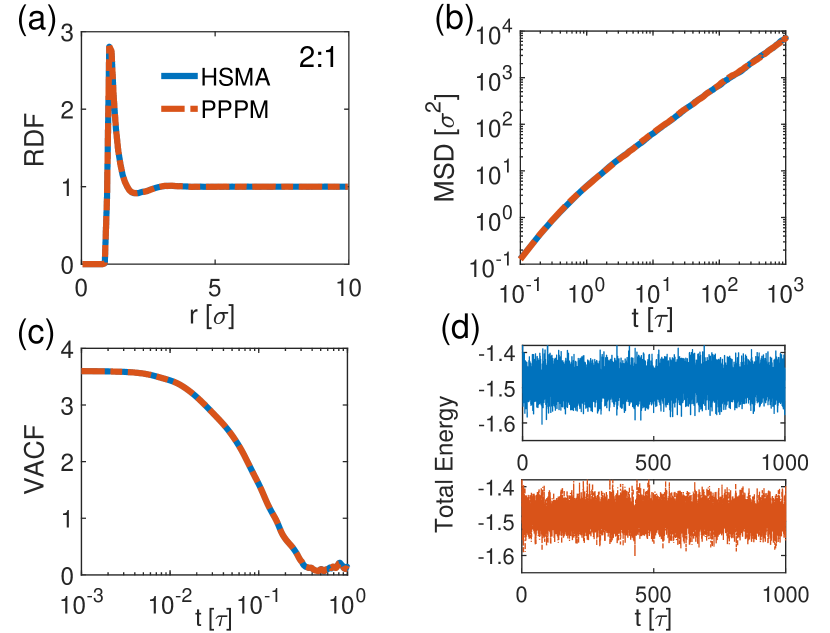
Figure 5: Accuracy comparison in 2:1 electrolytes. The simulation results from the PPPM (red dash-dot line) and HSMA (blue solid line) in electrolytes. (a): The radial distribution function of cation-anion in electrolytes. (b): The mean square displacement of cation in electrolytes. (c): The velocity auto correlation function of cation in electrolytes. (d): The total energy (unit: $\varepsilon_{\text{LJ}}$) of the system.

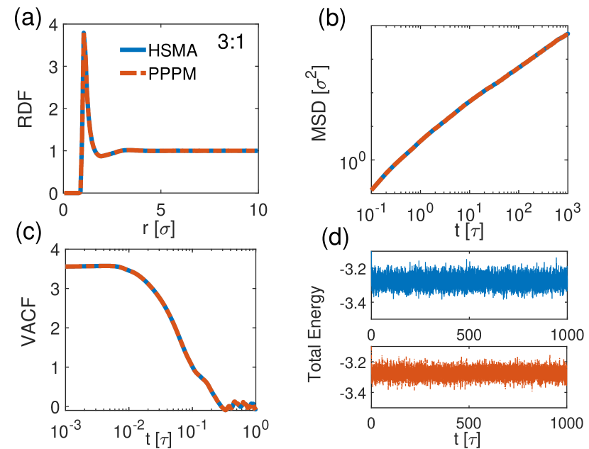
Figure 6: Accuracy comparison in 3:1 electrolytes. The simulation results from the PPPM (red dash-dot line) and HSMA (blue solid line) in electrolytes. (a): The radial distribution function of cation-anion in electrolytes. (b): The mean square displacement of cation in electrolytes. (c): The velocity auto correlation function of cation in electrolytes. (d): The total energy (unit: $\varepsilon_{\text{LJ}}$) of the system.

4.2 SPC/E bulk water

We also examine the structure of pure water by employing the classical SPC/E model [49]. The cubic simulation box has a dimension of 5.60 nm with periodic boundary conditions and 17496 atoms were placed within the central cell. The equilibrium temperature is set to $T=298K$. The equilibration process was carried out for 50 ns in $NPT$ ensemble, followed by $NVT$ MD simulation of 100ns for data collecting with the PPPM and HSMA3D, respectively. Here, six important quantities, namely the RDF of oxygen-oxygen, oxygen-hydrogen, and hydrogen-hydrogen, the MSD, the VACF, and the total energy of the whole system are examined to characterize the structure and dynamics of the SPC/E water.

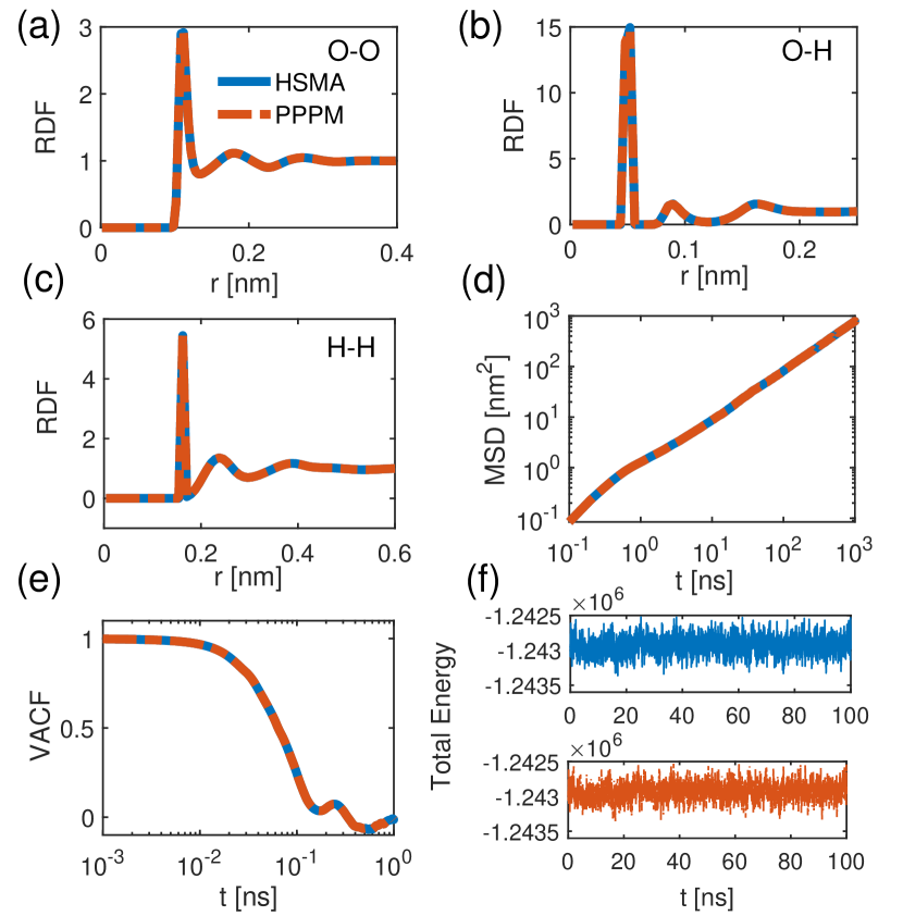
Figure 7: Accuracy comparison in SPC/E pure water system. The simulation results from the PPPM (red dash-dot line) and HSMA (blue solid line) in bulk water. (a-c): The radial distribution function of oxygen-oxygen, oxygen-hydrogen, and hydrogen-hydrogen in water molecules, respectively. (d): The mean square displacement of oxygen in water molecules. (e): The velocity auto correlation function of oxygen in water molecules. (f): The total energy (unit: Kcal/M) of the system. Note that in (f), the mean energy produced by the HSMA and the PPPM is -1243057.9 and -12431058.1, and the variance of energy produced by the HSMA and the PPPM is 431035.2 and 431854.1, respectively.

The RDF of oxygen-oxygen, oxygen-hydrogen, and hydrogen-hydrogen atom pairs are presented in Fig. 7(a)-(c), in agreement with previous computational investigations [50]. Note, however, that the first peak of the RDF of oxygen-hydrogen and hydrogen-hydrogen in Ref. [50] is missed because the oxygen and hydrogen within the same water molecule is not considered. The MSD of the oxygen in water molecules is shown in Fig. 7(d), describing the translational motion on different time scales. The VACF and the total energy of the whole system, are provided in Fig. 7(e) and Fig. 7(f). In all the panels above, we find an excellent agreement between HSMA3D and the PPPM.

4.3 Primitive electrolytes between dielectric interfaces

To demonstrate the accuracy of the HSMA2D for planar dielectric interfaces in a MD simulation, we study the primitive monovalent and divalent electrolytes confined between two dielectric interfaces. We assume that the top and bottom substrates have the same permittivity, i.e., $\gamma_{\text{up}}=\gamma_{\text{low}}=\gamma=0.939$. The shifted-truncated LJ potential is used for modeling excluded-volume effects as in Sec. 4.1. The system has dimensions $L_{x}=100\sigma$, $L_{y}=100\sigma$, and $L_{z}=50\sigma$. The monovalent and divalent electrolytes contain $218$, $109$ cations and $218$, $218$ anions, respectively. The ions are immersed in continuum solvent characterized by a Bjerrum length $\ell_{\text{B}}=3.5\sigma$. The ions are confined by purely repulsive shifted-truncated LJ walls ($\varepsilon_{\text{ion-wall}}=k_{\text{B}}T$; $\sigma_{\text{ion-wall}}=0.5\sigma$) at $z=-25\sigma$ and $z=25\sigma$. The MD simulations utilize a time step $0.005\tau$. Integration proceeds via the time-reversible measure-preserving Verlet and rRESPA integrators and the simulations are performed in the $NVT$ ensemble, where the temperature is controlled by a Nos$\acute{\text{e}}$-Hoover thermostat with damping time $0.05\tau$. The simulation initially proceeds for $5\times 10^{5}$ time steps for equilibration, followed by a production period which occupies $10^{8}$ time steps.

Ion distributions of monovalent and divalent electrolytes under dielectric confinement are presented in Fig. 8(a) and (b), calculated by HSMA2D along with a comparison to the ICM-PPPM algorithm [41]. As expected, repulsive polarization results in ion depletion. Such dielectric effects on the ion distribution are particularly strong for divalent salt. We observe that the HSMA2D and ICM-PPPM produce statistically identical distributions, confirming the correct implementation of HSMA2D in LAMMPS.

Figure 8: Distributions of ion density of (a) a monovalent electrolyte and (b) a divalent electrolyte between polarizable interfaces with $\gamma=0.939$. We use different symbols and lines for the results of different kinds of ions of HSMA2D (solid multiple signs for cation and solid squares for anion) and of ICM-PPPM (solid line for cation and dash-dotted line for anion), and different colors to present different methods (blue for HSMA2D, and red for ICM-PPPM). The distributions obtained using HSMA2D and ICM-PPPM overlap within statistical accuracy. The expected ion depletion near insulating interfaces are borne out by the simulations.

5 Performance analysis

The performance comparison of performance between HSMA and the PPPM was carried out by using the MD engine of LAMMPS (version 7Aug2019) on primitive electrolytes, all-atom simulation of SPC/E water, and electrolytes confined by two parallel dielectric interfaces. To access a fair comparison, the estimated relative force errors $\Delta$ is chosen as $10^{-5}$. The parameters of the PPPM are chosen automatically in LAMMPS based on the error estimates [51]. The parameters of HSMA are chosen the same as in Sec. 3.2. Because HSMA is a package accelerated by a hybrid MPI plus OpenMP parallelization, the version of the PPPM is chosen as the optimized multi-threaded version in the USER-OMP package of LAMMPS for the same acceleration support. Our HSMA package provides two optimized options. The first is vectorization for directly compute by using AVX512 instructions. The second is the FMM for achieving a linear complexity. The former is more efficient for a small system, while the latter is a general choice for a large system. The publicly available software package FMM3D [52, 53] is adopted for the FMM acceleration.

The computations in this article were performed on the $\pi$ 2.0 cluster supported by the Center for High Performance Computing at Shanghai Jiao Tong University. Each CPU node contains two Intel Xeon Scalable Cascade Lake 6248 (2.5GHz, 20 cores) and 12 $\times$ Samsung 16GB DDR4 ECC REG 2666 memory. The “intel-parallel-studio/cluster.2020.1-intel-19.1.1” is used as the compiler and the LAMMPS is compiled using “make intel$\_$cpu$\_$intelmpi”.

We characterize the CPU performance and parallel efficiency of the implemented package in LAMMPS for a practical simulation study on SPC/E pure water systems, which is commonly used system in the all-atom simulation, and monovalent electrolytes confined by two parallel dielectric interfaces. To reduce the communication cost as much as possible, we employ few MPI ranks but more OpenMP threads as recommended in section 3.2.

5.1 Time performance of HSMA3D

The CPU time of the SPC/E water system as a function of the number of atoms $N$ for different methods is shown in Fig. 9. For this, we use $1$ MPI rank with $40$ OpenMP threads. The simulations of the system were conducted for $2000$ steps to estimate the average CPU time per step. The density of water molecules is fixed to $1~{}\text{g/c}\text{m}^{3}$. The real-space cutoff for LJ potential is set to $10\mathring{\text{A}}$ for both HSMA and PPPM. Moreover, for the PPPM, we perform a set of simulations with varying cutoff for real-space Coulomb interaction to obtain the optimal CPU time. As illustrated in Fig. 9, HSMA has attractive performance for various sizes of systems, from $10^{2}$ to $10^{6}$. When $N<10^{4}$, HSMA is faster due to the small prefactor of direct compute. However, because of the $O(N^{2})$ complexity, the performance of PPPM exceeds HSMA when $N>10^{4}$. Note that for the choice of acceleration methods of HSMA, we choose the faster one and label the breakeven point in the figure. After this breakeven point (about $3\times 10^{4}$), the FMM is employed instead of direct vectorization thus achieves an $O(N)$ linear complexity. The HSMA and PPPM have the almost same performance when $N>10^{5}$. Fig. 9(b) shows the strong scaling analysis of the HSMA for different ways of acceleration. The testing system contains $10^{5}$ atoms. The parallel efficiency decreases as the number of CPU cores increases, as expected. Both vectorization and FMM have attractive parallel efficiency. The parallel efficiency of direct vectorization is slightly larger than FMM, because the complex data structure contains more serial computational parts.

In our previous work [42, 43], the breakeven point between the FMM and direct computation is about $3000$. However, we find that the breakeven point moves up by utilizing the vectorization technique for optimization. This increment may alter if the FMM code could also include vectorization. We note that the above comparison is merely an indication of the relative efficiency; a complete comparison also requires taking into account different particle distributions, and other issues [20].

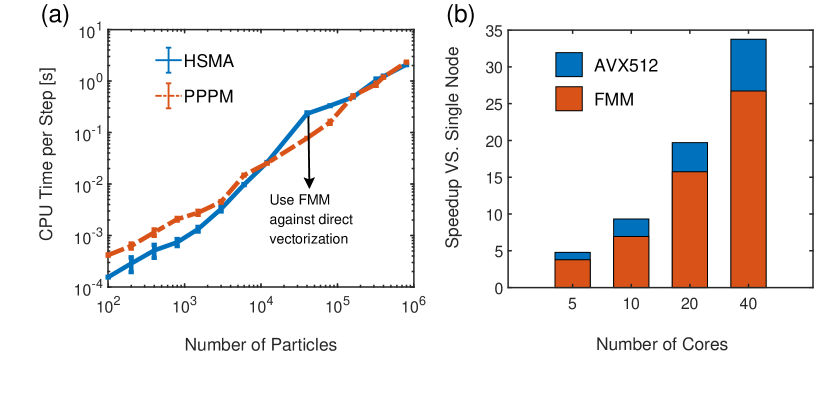
Figure 9: Performance analysis in SPC/E pure water system. (a) Average CPU time per simulation step as a function of the particle number of pure water systems. $1$ MPI rank with 40 OpenMP threads are employed for this test. Blue solid line : HSMA with $\Delta=10^{-5}$. Red dash-dotted line : PPPM with $\Delta=10^{-5}$. Note that for the choice of acceleration methods of HSMA, we choose the faster one and label the breakeven point in the figure. (b) Speedup on multiple compute nodes versus single node calculations for the system contains $10^{5}$ atoms for different ways of acceleration of HSMA. Blue : Direct computation with acceleration of AVX512. Red : Acceleration by using the FMM.

5.2 Time performance of HSMA2D

The CPU performance and parallel efficiency of the implemented HSMA2D in LAMMPS are examined for a practical simulation study on monovalent electrolytes confined by two parallel plates. To our knowledge, there are some methods implemented in LAMMPS for dielectric interfaces [41, 54] but, no package with the FMM or vectorization optimization exists. Due to this reason, we compare HSMA2D with the PPPM with slab correction (PPPM2D) method which is fully optimized in LAMMPS. Note that the system confined by two parallel plates is a specical case of dielectric system with no dielectric mismatch, i.e., $\gamma=0$. The real-space cutoff for PPPM2D is set to $10\sigma$.

The average CPU time per simulation step as a function of the particle number of monovalent electrolyte is shown in Fig. 10. Note that we fix the box size and alter the density of electrolytes in this test. The simulations of the system were conducted for 2000 steps to estimate the average CPU time per step. $1$ MPI rank with $40$ OpenMP threads is performed for this test. Note that for the choice of acceleration methods of HSMA, we choose the faster one and label the breakeven point (about $2\times 10^{4}$) in the figure. As shown in Fig. 10(a), HSMA2D is significantly faster (about $1.5$ magnitude) at low particle numbers, but beyond the break-even points of $N\approx 3\times 10^{4}$ (occpies about $3.1\%$ ion volume fraction), the PPPM2D and the HSMA2D have nearly the same performance. This is because the direct vectorization is used when $N\leq 2\times 10^{4}$, resulting in high efficiency but $O(N^{2})$ complexity. We do not test larger systems ($N>10^{5}$) because of the more memory allocation than the accessible memory per node. It can be predicted that the HSMA2D with the FMM acceleration will have more advantages if the system is larger than $10^{5}$ due to the linear scaling. Fig. 10(b) shows the strong scaling analysis of the HSMA2D for different ways of acceleration. The testing system contains $10^{5}$ atoms. The parallel efficiency decreases as the number of CPU cores increases, as expected. Both vectorization and the FMM have attractive parallel efficiency and a slight loss than the results in fully periodic system as shown in Fig. 9(a) thanks to the complicated calculation of the 2D-dilation formula.

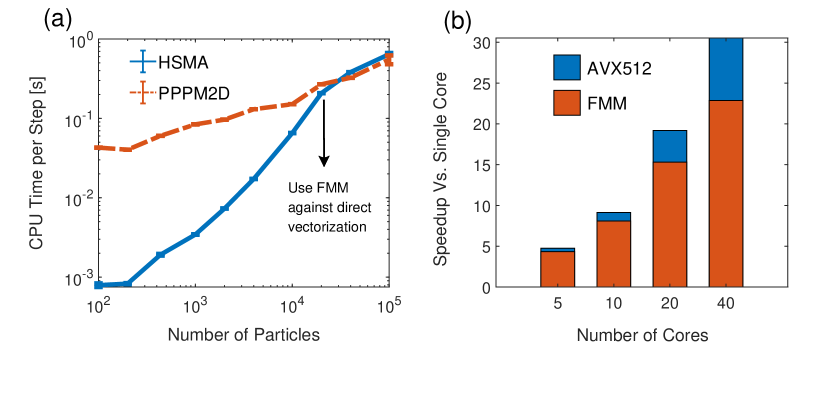
Figure 10: Performance analysis in monovalent electrolyte confined by two dielectric interfaces. We fix the dimensions as $L_{x}=100\sigma$, $L_{y}=100\sigma$, and $L_{z}=50\sigma$ then change the ion density of electrolyte. (a) Average CPU time per simulation step as a function of the different ranges of monovalent electrolyte. $1$ MPI rank with 40 OpenMP threads are employed for this test. Blue solid line : HSMA with $\Delta=10^{-5}$. Red dash-dotted line : PPPM2D with $\Delta=10^{-5}$ and kspace$\_$modify slab 4 command. Note that for the choice of acceleration methods of HSMA, we choose the faster one and label the breakeven point in the figure. (b) Speedup on multiple compute nodes versus single node calculations for system contains $10^{5}$ atoms for different ways of acceleration of HSMA. Blue : Direct computation with acceleration of AVX512. Red : Acceleration by using the FMM.

6 Conclusion

We have implemented HSMA methods for modeling electrostatic interactions of fully periodic and partially periodic systems in LAMMPS. We have validated our implementation by comparing the results of primitive electrolytes and all-atom pure water to those obtained by other numerical methods. The codes are released as an open-source USER-HSMA package which can be easily compiled into LAMMPS. We have compared the CPU performance and the parallel efficiency of the implemented HSMA for practical simulations, showing the attractive performance and good strong scaling. The HSMA for fully/partially periodic systems is very efficient for both small and large particle numbers. This implementation allows efficient and accurate coarse-grained and all-atom molecular dynamics simulations of a broad variety of charged systems, such as, polyelectrolytes, ionic liquids, proteins, or membranes.

7 Acknowledgments and Competing interests

The authors acknowledge the Center for High Performance Computing at Shanghai Jiao Tong University for the computing resources. The work of J. Liang and Z. Xu was partially supported by NSFC (grant Nos. 12071288) and Shanghai Science and Technology Commission (grant No. 20JC1414100). All the authors have declared no competing interest.

References

- [1] G. C. L. Wong, J. X. Tang, A. Lin, Y. Li, P. A. Janmey, C. R. Safinya, Hierarchical self-assembly of F-actin and cationic lipid complexes: Stacked three-layer tubule networks, Science 288 (2000) 2035–2039.
- [2] M. A. Boles, M. Engel, D. V. Talapin, Self-assembly of colloidal nanocrystals: From intricate structures to functional materials, Chem. Rev. 116 (18) (2016) 11220–11289.
- [3] Y. Burak, G. Ariel, D. Andelman, Onset of DNA aggregation in presence of monovalent and multivalent counterions, Biophys. J. 85 (2003) 2100–2110.
- [4] H.-X. Zhou, X. Pang, Electrostatic interactions in protein structure, folding, binding, and condensation, Chem. Rev. 118 (4) (2018) 1691–1741.
- [5] M. Lund, B. Jönsson, On the charge regulation of proteins, Biochemistry 44 (15) (2005) 5722–5727.
- [6] M. Lund, B. Jönsson, Charge regulation in biomolecular solution, Q. Rev. Biophys. 3 (2013) (2019) 265–281.
- [7] I. Borukhov, D. Andelman, H. Orland, Steric effects in electrolytes: A modified Poisson–Boltzmann equation, Phys. Rev. Lett. 79 (3) (1997) 435–438.
- [8] A. R. J. Silalahi, A. H. Boschitsch, R. C. Harris, M. O. Fenley, Comparing the predictions of the nonlinear Poisson–Boltzmann equation and the ion size-modified Poisson–Boltzmann equation for a low-dielectric charged spherical cavity in an aqueous salt solution, J. Chem. Theory Comput. 6 (12) (2010) 3631–3639.
- [9] D. Frenkel, B. Smit, Understanding Molecular Simulation, 2nd Edition, Academic, San Diego, 2002.
- [10] P. P. Ewald, Die Berechnung optischer und elektrostatischer Gitterpotentiale, Ann. Phys. (Leipzig) 369 (3) (1921) 253–287.
- [11] R. W. Hockney, J. W. Eastwood, Computer simulation using particles, crc Press, 1988.
- [12] S. Jin, L. Li, Z. Xu, Y. Zhao, A random batch Ewald method for particle systems with Coulomb interactions, ArXiv preprint arXiv:2010.01559 (2020).
- [13] J. Barnes, P. Hut, A hierarchical O(NlogN) force-calculation algorithm, Nature 324 (6096) (1986) 446–449.
- [14] L. Greengard, V. Rokhlin, A fast algorithm for particle simulations, J. Comp. Phys. 73 (2) (1987) 325–348.
- [15] E. Pollock, J. Glosli, Comments on P3M, FMM, and the Ewald method for large periodic Coulombic systems, Comput. Phys. Commun. 95 (2-3) (1996) 93–110.
- [16] W. M. Brown, A. Kohlmeyer, S. J. Plimpton, A. N. Tharrington, Implementing molecular dynamics on hybrid high performance computers–particle-particle particle-mesh, Comput. Phys. Commun. 183 (3) (2012) 449–459.
- [17] I. Bush, I. Todorov, W. Smith, A DAFT DL_POLY distributed memory adaptation of the Smoothed Particle Mesh Ewald method, Comput. Phys. Commun. 175 (5) (2006) 323–329.
- [18] S. Plimpton, Fast parallel algorithms for short-range molecular dynamics, J. Comp. Phys. 117 (1) (1995) 1–19.
- [19] H. J. Berendsen, D. van der Spoel, R. van Drunen, GROMACS: a message-passing parallel molecular dynamics implementation, Comput. Phys. Commun. 91 (1-3) (1995) 43–56.
- [20] A. Arnold, F. Fahrenberger, C. Holm, O. Lenz, M. Bolten, H. Dachsel, R. Halver, I. Kabadshow, F. Gähler, F. Heber, J. Iseringhausen, M. Hofmann, M. Pippig, D. Potts, G. Sutmann, Comparison of scalable fast methods for long-range interactions, Phys. Rev. E 88 (2013) 063308.
- [21] R. Messina, Effect of image forces on polyelectrolyte adsorption at a charged surface, Phys. Rev. E 70 (2004) 051802.
- [22] K. Barros, E. Luijten, Dielectric effects in the self-assembly of binary colloidal aggregates, Phys. Rev. Lett. 113 (2014) 017801.
- [23] A. P. dos Santos, M. Girotto, Y. Levin, Simulations of polyelectrolyte adsorption to a dielectric like-charged surface, J. Phys. Chem. B 120 (39) (2016) 10387–10393.
- [24] H. Wu, H. Li, F. J. Solis, M. Olvera de la Cruz, E. Luijten, Asymmetric electrolytes near structured dielectric interfaces, J. Chem. Phys. 149 (2018) 164701.
- [25] J. Yuan, H. S. Antila, E. Luijten, Structure of polyelectrolyte brushes on polarizable substrates, Macromolecules 53 (8) (2020) 2983–2990.
- [26] M. Ma, Z. Gan, Z. Xu, Ion structure near a core-shell dielectric nanoparticle, Phys. Rev. Lett. 118 (7) (2017) 076102.
- [27] B. Zhang, Y. Ai, J. Liu, S. W. Joo, S. Qian, Polarization effect of a dielectric membrane on the ionic current rectification in a conical nanopore, J. Phys. Chem. C 115 (50) (2011) 24951–24959.
- [28] H. S. Antila, E. Luijten, Dielectric modulation of ion transport near interfaces, Phys. Rev. Lett. 120 (2018) 135501.
- [29] J. Yuan, H. S. Antila, E. Luijten, Dielectric effects on ion transport in polyelectrolyte brushes, ACS Macro Lett. 8 (2019) 183–187.
- [30] D. Boda, D. Gillespie, W. Nonner, D. Henderson, B. Eisenberg, Computing induced charges in inhomogeneous dielectric media: Application in a Monte Carlo simulation of complex ionic systems, Phys. Rev. E 69 (2004) 046702.
- [31] K. Barros, D. Sinkovits, E. Luijten, Efficient and accurate simulation of dynamic dielectric objects, J. Chem. Phys. 140 (2014) 064903.
- [32] X. Jiang, J. Li, X. Zhao, J. Qin, D. Karpeev, J. Hernandez-Ortiz, J. J. de Pablo, O. Heinonen, An and parallel approach to integral problems by a kernel-independent fast multipole method: Application to polarization and magnetization of interacting particles, J. Chem. Phys. 145 (6) (2016) 064307.
- [33] H. Wu, E. Luijten, Accurate and efficient numerical simulation of dielectrically anisotropic particles, J. Chem. Phys. 149 (2018) 134105.
- [34] V. Jadhao, F. J. Solis, M. Olvera de la Cruz, Simulation of charged systems in heterogeneous dielectric media via a true energy functional, Phys. Rev. Lett. 109 (22) (2012) 223905. doi:10.1103/PhysRevLett.109.223905.
- [35] V. Jadhao, F. J. Solis, M. Olvera de la Cruz, A variational formulation of electrostatics in a medium with spatially varying dielectric permittivity, J. Chem. Phys. 138 (5) (2013) 054119.
- [36] Z. Gan, S. Jiang, E. Luijten, Z. Xu, A hybrid method for systems of closely spaced dielectric spheres and ions, SIAM J. Sci. Comp. 38 (3) (2016) B375–B395.
- [37] W. Thomson, Geometrical investigations with reference to the distribution of electricity on spherical conductors, Camb. Dublin Math. J. 3 (1848) 141–148.
- [38] S. Tyagi, A. Arnold, C. Holm, ICMMM2D: An accurate method to include planar dielectric interfaces via image charge summation, J. Chem. Phys. 127 (15) (2007) 154723.
- [39] S. Tyagi, A. Arnold, C. Holm, Electrostatic layer correction with image charges: A linear scaling method to treat slab systems with dielectric interfaces, J. Chem. Phys. 129 (20) (2008) 204102.
- [40] A. P. dos Santos, Y. Levin, Electrolytes between dielectric charged surfaces: Simulations and theory, J. Chem. Phys. 142 (19) (2015) 194104.
- [41] J. Yuan, H. S. Antila, E. Luijten, Particle–particle particle–mesh algorithm for electrolytes between charged dielectric interfaces, J. Chem. Phys. 154 (9) (2021) 094115.
- [42] Q. Zhao, J. Liang, Z. Xu, Harmonic surface mapping algorithm for fast electrostatic sums, J. Chem. Phys. 149 (8) (2018) 084111.
- [43] J. Liang, J. Yuan, E. Luijten, Z. Xu, Harmonic surface mapping algorithm for molecular dynamics simulations of particle systems with planar dielectric interfaces, J. Chem. Phys. 152 (13) (2020) 134109.
- [44] S. J. Plimpton, Fast parallel algorithms for short-range molecular dynamics, J. Comp. Phys. 117 (1995) 1–19.
- [45] N. A. Gumerov, R. Duraiswami, A method to compute periodic sums, J. Comp. Phys. 272 (2014) 307–326.
- [46] D. Occorsio, G. Serafini, Cubature formulae for nearly singular and highly oscillating integrals, Calcolo 55 (1) (2018) 1–33.
- [47] S. Blair-Chappell, A. Stokes, Parallel programming with Intel Parallel Studio XE, John Wiley & Sons, 2012.
- [48] J. Liang, P. Liu, Z. Xu, A high-accurate fast Poisson solver based on harmonic surface mapping algorithm, accepted by Communications in Computational Physics (2021).
- [49] H. Berendsen, J. Grigera, T. Straatsma, The missing term in effective pair potentials, J. Phys. Chem. 91 (24) (1987) 6269–6271.
- [50] P. Mark, L. Nilsson, Structure and dynamics of the TIP3P, SPC, and SPC/E water models at 298 K, J. Phys. Chem. A 105 (43) (2001) 9954–9960.
- [51] M. Deserno, C. Holm, How to mesh up Ewald sums. II. An accurate error estimate for the particle–particle–particle–mesh algorithm, J. Chem. Phys. 109 (18) (1998) 7694–7701.
- [52] H. Cheng, L. Greengard, V. Rokhlin, A fast adaptive multipole algorithm in three dimensions, J. Comp. Phys. 155 (2) (1999) 468–498.
- [53] L. F. Greengard, J. Huang, A new version of the fast multipole method for screened Coulomb interactions in three dimensions, J. Comp. Phys. 180 (2) (2002) 642–658.
- [54] T. D. Nguyen, H. Li, D. Bagchi, F. J. Solis, M. O. de la Cruz, Incorporating surface polarization effects into large-scale coarse-grained molecular dynamics simulation, Comput. Phys. Commun. 241 (2019) 80–91.