Boltzmann Tuning of Generative Models

Abstract

The paper focuses on the a posteriori tuning of a generative model in order to favor the generation of good instances in the sense of some external differentiable criterion. The proposed approach, called Boltzmann Tuning of Generative Models (BTGM), applies to a wide range of applications. It covers conditional generative modelling as a particular case, and offers an affordable alternative to rejection sampling. The contribution of the paper is twofold. Firstly, the objective is formalized and tackled as a well-posed optimization problem; a practical methodology is proposed to choose among the candidate criteria representing the same goal, the one best suited to efficiently learn a tuned generative model. Secondly, the merits of the approach are demonstrated on a real-world application, in the context of robust design for energy policies, showing the ability of BTGM to sample the extreme regions of the considered criteria.

1 Introduction

Deep generative models, including Variational Auto-Encoders (VAEs) (Kingma and Welling, 2014; Rezende et al., 2014), Generative Adversarial Networks (GANs) (Goodfellow et al., 2014), and Normalizing Flows (Rezende and Mohamed, 2015), have been used in a number of ways for (semi)-supervised learning and design. Their usage ranges from robustifying classifiers (Kingma et al., 2014; Li et al., 2019) to achieving anomaly detection (Pidhorskyi et al., 2018; Choi et al., 2019)) or solving undetermined inverse problems (Ardizzone et al., 2019), from super-resolution of images (Ledig et al., 2017) to computer-assisted creative design (Park et al., 2019). In most cases, the fine-tuning of the generative model is seamlessly integrated within the learning process: through the design of the latent representation (Radford et al., 2016; Mathieu et al., 2016) or through the loss itself, e.g. leveraging labelled information to train conditional generative models (van den Oord et al., 2016) (more in section 2).

This paper tackles the a posteriori tuning of a trained generative model, aimed at favoring the generation of good samples in the sense of a given criterion. The applicative motivation for the proposed approach comes from the design of energy safety policies. In this context, an infrastructure must be tested against a host of diverse production and consumption scenarios, and specifically against their associated consumption peaks. One applicative goal of the proposed approach, called Boltzmann Tuning of Generative Models (BTGM), is to address this problem by generating consumption curves directly sampling the desired top quantiles of the aggregated consumption distribution.

This paper considers the general setting defined by a trained generative model and some criterion $f$, with the goal of generating samples biased toward maximizing $f$. This goal is formalized as a constrained optimization problem in the considered distribution space, and a first contribution is to show how to soundly and effectively tackle this problem within the variational inference framework, assuming the differentiability of the criterion  (section 3). The proposed BTGM approach can be applied on the top of any deep generative model, covering conditional generative models (van den Oord et al., 2016) as a particular case. It also opens some perspectives in privacy-sensitive domains, e.g. to generate samples in critical and data-poor regions (see also Dash et al. (2020)). In practice, BTGM offers an affordable and, to our best knowledge, new alternative to rejection sampling.

Most generally, BTGM is an attempt toward reconciling data-driven models (here, the generative model learned from extensive data) on the one hand, and analytical, interpretable knowledge (here, the characterization of $f$) on the other hand. While ML traditionally focuses on cases where knowledge/specification is better conveyed through data, some specifications are better conveyed analytically, particularly so when they are poorly illustrated in the data (see also Bessiere et al. (2017)). The challenge is to take advantage of both raw data and analytical criteria in an integrated way. Along this line, a second contribution of the paper regards how to formulate the user’s criterion $f$ in the most effective way. Indeed the objective can be formulated in many different ways, up to monotonous transformations of $f$. In order to avoid determining the best formulation of the criterion along a tedious trial-and-error phase, an indicator based on the analysis of the underlying optimization process is defined, enabling the comparison of candidate criteria w.r.t. the tuning of the generative model at hand.

Section 4 presents several case studies to illustrate the merits and flexibility of the approach: recovering conditional generative modeling (4.1), comparing candidate criteria (4.2), showing the flexibility of the approach in the energy consumption modeling domain (4.3) and investigating the a posteriori deblurring of a generative model (4.4).

2 Related work

Probability distribution learning is most generally tackled within the Variational Inference (VI) framework. VI being also at the core of the proposed approach, it is presented in section 3.2 in a unified way, to both learn a probability distribution from raw data, and tune an existing probability distribution along an analytical criterion.

The current trends in generative modelling mostly leverage the deep learning efficiency and flexibility to estimate a probability distribution from data, supporting an efficient sampling mechanism (Kingma and Welling, 2014; Rezende et al., 2014; Goodfellow et al., 2014; Rezende and Mohamed, 2015). Most approaches rely on the introduction of a latent space, whose samples are decoded into a data space. The generative model is trained to optimize a goodness-of-fit criterion on the original data. In VAEs (Kingma and Welling, 2014), the goodness of fit is the log-likelihood (LL) of the initial data, estimated using the Evidence Lower Bound (ELBO) (Bishop et al., 1998), as the distribution involves an unknown/unmanageable normalization constant. In GANs (Goodfellow et al., 2014), the goodness of fit criterion is replaced by a 2-sample test, adversarially training the generator and a discriminator estimating whether the generated examples can be discriminated from the original samples.

Distribution spaces. How to make the generative model space flexible enough to accurately approximate the true distribution is mostly handled through using richer latent spaces and/or inference models (Burda et al., 2016; van den Oord et al., 2017; Roy et al., 2018; Razavi et al., 2019; Huang et al., 2019; Mathieu et al., 2019a; Kalatzis et al., 2020; Skopek et al., 2020). The modelling of multi-mode distributions can also be tackled using continuous and discrete latent variables (Jang et al., 2017; Vahdat et al., 2018). Specific architectures are designed to exploit the specifics of the data structure, such as Wavenet or Magenta for signal processing (Oord et al., 2016b; Roberts et al., 2018) or PixelRNN/CNN for images (Oord et al., 2016a; Salimans et al., 2017), enabling the data likelihood to be explicitly computed and optimized. Normalizing Flows (Rezende and Mohamed, 2015; Dinh et al., 2015) also proceed by gradually complexifying a distribution, with the particularity that each layer is invertible and enables its Jacobian to be analytically determined, thereby supporting the approximation of the posterior distributions (Dinh et al., 2017; Kingma et al., 2017; Ardizzone et al., 2019; Chen et al., 2020).

Loss functions. The loss function encapsulates the goodness of fit criterion. Many VAE variants focus on the reformulation of the loss to finely control the trade-off between the reconstruction quality and encoding compression (Higgins et al., 2017; Rezende and Viola, 2018; Alemi et al., 2018; Mathieu et al., 2019b). The loss design also aims to avoid pitfalls, notably in terms of instability or mode dropping (Arjovsky et al., 2017) with GANs; other distances between the generated and the original distributions (Nowozin et al., 2016; Arjovsky et al., 2017) and/or more elaborate model architectures (Sajjadi et al., 2018; Shaham et al., 2019; Torkzadehmahani et al., 2019) have thus been investigated.

Refining Generative Models. Most generally, the refinement of generative models is based on exploiting supervised information to build conditional models (Mirza and Osindero, 2014; Sohn et al., 2015; van den Oord et al., 2016; Jaiswal et al., 2019). Another strategy is to use several data samples, within a domain adaptation or multi-task setting (Ganin et al., 2016), and to learn coupled generative models (Chu et al., 2017). Most generally, the customization and refinement of generative models builds upon one or several datasets, exploiting prior knowledge about their features (labels), or about the relationships between the datasets (Courty et al., 2017).

The alternative explored by BTGM is to use high-level, analytical information, expressed via criteria, to refine a generative model. On the positive side, this approach is flexible and does not depend on the regions of interest of the instance space to be "sufficiently" represented in the dataset(s). On the negative side, the approach might be too flexible, in the sense that the regions of interest might be specified in a number of ways, although not all specifications are equally easy to deal with. We shall return to this point in section 4.2.

3 Boltzmann Tuning of Generative Models

Let $p$ and $f$ respectively denote the initial generative model defined on the sample space $\mathcal{X}\subset\mbox{$\mathbb{R}$}^{d}$, and the criterion of interest ($f:\mathcal{X}\mapsto\mbox{$\mathbb{R}$}$). It is assumed wlog that the generative model should be biased toward regions where $f$ takes high values. The sought biased generative model $q$ is expressed as the solution of a constrained optimization problem: maximizing the expectation of $f$ under $q$, subject to $q$ remaining "sufficiently" close to $p$ in the sense of their Kullback-Leibler divergence:

$$\mbox{Find~{}}q=\arg\max\mathbb{E}_{q}[f]~{}s.t.~{}D_{KL}(q\||p)\leq C_{D}$$ (1)

with $C_{D}$ a positive constant. The Lagrangian $\mathcal{L}$ associated to this primal constrained optimization problem is, with $\lambda$ the Lagrange multiplier accounting for the constraint:

$$\mathcal{L}(q)=\int_{\mathcal{X}}q(x)f(x)dx+\lambda\int_{\mathcal{X}}q(x)\log\frac{q(x)}{p(x)}dx$$ (2)

reaching its optimum for:

$$q_{\beta}(x)=\frac{1}{Z(\beta)}p(x)e^{\beta f(x)}$$ (3)

with $\beta=1/\lambda$ and $Z(\beta)$ the normalization constant. BTGM tackles the dual optimization problem of minimizing $D_{KL}(q||p)$ subject to $\mathbb{E}_{q}f$ being greater than some constant $C_{f}$, yielding solution $q_{\beta}$ for some $\beta$ depending on $C_{f}$ (below):

$$q_{\beta}=\mathop{\arg\max}_{q}\;\beta\,\mathbb{E}_{q}f-D_{KL}(q\|p)$$ (4)

3.1 Finding $\beta$

Varying the strength of the bias, from no bias ($\beta=0$ yields $q_{\beta}=p$) to $\beta=\infty$ (with $q_{\beta}$ with support in the optima of $f$) yields a family of distributions, the Pareto front associated to the maximization of $\mathbb{E}_{q}f$ and minimization of $D_{KL}(q\|p)$. Simple calculations yield (Appendix A):

$$\frac{d}{d\beta}D_{KL}(q_{\beta}\|p)=\beta Var_{q_{\beta}}(f)\quad\text{and}\quad\frac{d}{d\beta}\mathbb{E}_{q_{\beta}}f=Var_{q_{\beta}}(f)$$ (5)

$D_{KL}(q_{\beta}\|p)$ and $\mathbb{E}_{q_{\beta}}f$ being strictly increasing functions of $\beta$, there exists a one-to-one mapping between the values of $D_{KL}(q_{\beta}\|p)$, and $\mathbb{E}_{q_{\beta}}f$, hence there exists a single $\beta$ value such that $q_{\beta}$ solves the constrained optimization problem. Further calculations yield the second order derivatives:

$$\frac{d^{2}}{d\beta^{2}}D_{KL}(q_{\beta}\|p)=Var_{q_{\beta}}(f)+\beta\mathbb{E}_{q_{\beta}}\left(f-\mathbb{E}_{q_{\beta}}f\right)^{3}\quad\frac{d^{2}}{d\beta^{2}}\mathbb{E}_{q_{\beta}}f=\mathbb{E}_{q_{\beta}}\left(f-\mathbb{E}_{q_{\beta}}f\right)^{3}$$ (6)

Note that any generative model $q_{\beta}$ enables by construction to empirically estimate the first three moments of $f$ under $q_{\beta}$, as well as $D_{KL}(q_{\beta}\||p)$. Plugging these estimates in Eqs. 5 and 6 and using second order optimization methods (Boyd and Vandenberghe, 2004) enables to quickly converge toward the desired value of $\beta$, i.e. such that $\mathbb{E}_{q_{\beta}}f=C_{f}$ (Alg. 1).

Algorithm 1 BTGM

  $\beta\leftarrow 0$

  repeat

     $q_{\beta}\leftarrow\mathop{\arg\max}_{q}\>\beta\mathbb{E}_{q}f-D_{KL}(q\|p)$ (section 3.2)

     Estimate $D_{KL}(q_{\beta}\|p)$, $\mathbb{E}_{q_{\beta}}f$, $Var_{q_{\beta}}(f)$ and $\mathbb{E}_{q_{\beta}}\left(f-\mathbb{E}_{q_{\beta}}f\right)^{3}$ by Monte-Carlo sampling

     Do a second-order update of $\beta$ using Eq. 5 and 6.

  until convergence of $\beta$

3.2 Building $q_{\beta}$

It is seen that Eq. 4 essentially defines a Variational Inference (VI) problem for each $\beta$ value. This problem is reformulated using the Evidence Lower Bound (ELBO) (Bishop et al., 1998):

$$q_{\beta}=\mathop{\arg\max}_{q}\;H(q)+\mathop{\mathbb{E}}_{x\sim q}\left[\beta f(x)+\log p(x)\right]$$ (7)

with $H(q)$ the entropy of $q$.

VI is intensively used for generative modelling, optimizing $q$ based on samples of the true distribution. The optimization of the ELBO (Ranganath et al., 2014) classically proceeds by leveraging stochastic optimization (Hoffman et al., 2013) or building upon the reparametrization trick (Kingma and Welling, 2014). The distribution space is chosen to efficiently approximate the posterior beyond the mean-field approximation, using low-rank Gaussian distributions (Ong et al., 2018), mixtures of Gaussian distributions (Gershman et al., 2012), or mixtures of an arbitrary number of distributions via boosting methods (Guo et al., 2017; Miller et al., 2017). An alternative is offered by Normalizing Flows, where the neural architecture achieves an invertible transformation enabling its Jacobian to be analytically determined, thereby supporting the approximation of the posterior distributions (Rezende and Mohamed, 2015; Kingma et al., 2017). The use of stochastic equations such as Langevin Monte-Carlo (Welling and Teh, 2011) can also be used to directly sample from the target distribution, without explicitly modelling it beforehand.

In the considered context, VI is used to tune an existing $q$ after $f$. Note that $q_{\beta}$ mostly specializes the initial generative model $p$ (as opposed to, exploring the very low probability regions of $p$, which would significantly degrade $D_{KL}(q_{\beta}\|p)$). Therefore $q_{\beta}$ will expectedly have its typical set (Nalisnick et al., 2019) roughly included in the typical set of $p$. Accordingly, $q$ is sought via deterministically perturbing the samples drawn according to $p$ (returning $x=g(\hat{x})$ with $\hat{x}$ sampled from $p$ and $g:\mathcal{X}\mapsto\mathcal{X}$ the perturbation). The Normalized Flow neural architecture is used to find $g$, for it makes its Jacobian explicit and easy to compute its determinant. With $J(g)$ the Jacobian matrix of $g$, it comes:

$$q(x)=p(\hat{x})\left|J(g)(\hat{x})\right|^{-1}$$ (8)

The optimization problem (Eq. 7) then reads:

$$\mbox{Find ~{}}g=\mathop{\arg\max}_{g}\mathop{\mathbb{E}}_{\hat{x}\sim p}\left[\beta f(g(\hat{x}))+\log p(g(\hat{x}))+\log\left|J(g)(\hat{x})\right|\right]$$ (9)

Some care is exercised at the initialization of Algorithm 1, setting $g$ very close to identity; the subsequent iterations proceed by warm-start, setting $g_{i}$ to the $g_{i-1}$ learned in the previous iteration.

3.3 Operating in latent space

The use of latent space is pervasive in generative modelling, notably for the sake of dimensionality reduction. The samples in the latent space (drawn after some simple, usually Gaussian, prior distribution $p(z)$) are mapped onto the instance space by the decoder module $p(x|z)$, in a deterministic ($x=\mathop{\mathbb{E}}dec(z)$) or probabilistic ($x\sim dec(z)$) way. The generative model is $p(x)=\int_{z}p(x|z)p(z)dz$.

Most interestingly, BTGM can operate in the latent space too, tuning the latent distribution $p(z)$ and yielding a tuned latent distribution noted $q_{\beta}(z)$. The sought tuned distribution $q_{\beta}(x)$ in the instance space is derived from $q_{\beta}(z)$ through the decoder module:

$$q_{\beta}(x)=\int_{z}p(x|z)q_{\beta}(z)dz$$

Operating on the latent space with a frozen decoder module offers several advantages. Firstly, the optimization criterion remains well defined, with $D_{KL}(q_{\beta}(z)\|p(z))$ an upper bound of $D_{KL}(q_{\beta}(x)\|p(x))$ (Appendix B). Secondly, conducting the optimization process in the latent space is easier and yields more robust results, due to the dimension of the latent space being usually lower than that of $\mathcal{X}$ by one or several orders of magnitude, and the generative distribution $p(z)$ being usually a simple one, e.g. $\mathcal{N}(0;Id)$. Last, freezing the decoder ensures that the support of the eventual generative model remains included in the support of the initial one. Formally, applying BTGM in the latent space amounts to replacing criterion $f$ by $\hat{f}$ defined on the latent space as:

$$\hat{f}(z)=\mathbb{E}_{x\sim p(x|z)}f(x)$$ (10)

4 Case studies

This section reports on four case studies conducted with BTGM. The code is available in supplementary material.

4.1 Conditional generative modelling

BTGM covers conditional generative modelling as a particular case. In a supervised learning context, with $h$ an (independently trained) classifier and $h(\ell|x)$ the probability of $x$ to be labelled as $\ell$, let criterion $f$ be set to $\log h(\ell|x)$ in order to bias the generative model toward class $\ell$. Model $q_{\beta}$ reads:

$$q_{\beta}(x)\propto p(x)h(\ell|x)^{\beta}$$ (11)

defining a standard conditional generative model of class $\ell$ for $\beta=1$ (assuming that $h(\ell|x)$ accurately estimates $p(\ell|x)$). Through parameter $\beta$, one can also control the fraction of samples closest to class $\ell$, by setting the constraint $D_{KL}(q_{\beta}\|p)\leq-log(\rho)$ with $\rho$ the mass of the desired fraction (Fig. 5, Appendix D). In the same spirit, BTGM can be used to debug classifier $h$, e.g. by generating samples in the ambiguous regions at the frontier of two or several classes (e.g. using as criterion$f$ the probability of the second most probable class or the entropy of the prediction of the classifier), and inspecting $h$ behavior in this region.

4.2 Assessing criteria ex ante

As said, an criterion $f$ can be represented in a number of ways, e.g. considering all $g\circ f$ with $g$ a monotonous function; still, the associated optimization problems (Eq. 7) are in general of varying difficulty. In order to facilitate the usage of BTGM and avoid a tedious trials and errors phase, some way of comparing a priori two criteria is thus desirable.

It is easy to see that the Pareto front of BTGM solutions (section 3.1) is invariant under affine transformations of $f$. In the following, any criterion $f$ is normalized via an affine transformation (below), yielding an expectation and variance under $p$ respectively set to $0$ and $1$.

Informally, the difficulty of the optimization problem reflects how much $p$ has to be transformed to match $q_{\beta}$. This difficulty can be quantified from the log ratio of $p$ and $q_{\beta}$, specifically measuring whether this log ratio is subject to fast variations. A measure of difficulty thus is the norm of $\nabla_{x}\log\frac{q_{\beta}(x)}{p(x)}$. Note that the distribution of this gradient norm can be empirically estimated:

$$\nabla_{x}\log\frac{q_{\beta}(x)}{p(x)}=\beta\nabla_{x}f(x)$$ (12)

Overall, samples generated from $p$ are used: i/ to normalize the candidate criteria; ii/ to estimate the distribution of their gradient norm; and iii/ to compare two criteria and prefer the one with more regular distribution, as defining a smoother optimization problem. This analysis extends to the tuning of generative models in latent space, replacing $f$ with $\hat{f}$ (Eq. 10).

The methodology is illustrated in the conditional modelling context (section 4.1), to compare the two criteria $f(x)=h(\ell|x)$ and $f(x)=log(h(\ell|x))$, respectively referred to as $f_{log.h}$ and $f_{h}$. The distribution of their gradients under $p$ is displayed on Fig. 1. The binned distribution of the gradient norms in latent space for all ten classes, is estimated from 10,000 samples (truncated for readability: the highest values for the gradient norm of $f_{h}$ go up to 60-100, to be compared to 10-15 for the gradient norm of $f_{log.h}$).

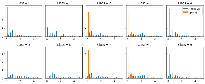
Figure 1: Comparing criteria$f_{log.h}$ (in blue) and $f_{h}$ (in orange) on MNIST: binned distribution of their gradient norms (better seen in color). The distribution tails are truncated for the sake of visualization, see text.

The distribution of the $f_{h}$ gradient norm shows a high mass on 0 with quite some high values, suggesting a complex optimization landscape with a number of plateaus (gradient norm 0) separated by sharp boundaries (high gradient norms). In opposition, the distribution of the $f_{log.h}$ gradient norm is flatter with a more compact support, suggesting a manageable optimization landscape where the gradient offers some (bounded) information in most regions. Accordingly, it is suggested $f_{log.h}$ is much more amenable to the tuning of the generative model than $f_{h}$, which is empirically confirmed (Appendix C). Overall, the proposed methodology allows to efficiently and inexpensively compare a priori candidate criteria, and retain the most convenient one.

4.3 A real-world case study

This section focuses on using BTGM as an alternative to rejection sampling on the real-world problem of smart grid energy management and dimensioning. For the sake of reproducibility, an experiment on MNIST along the same rejection sampling ideas is detailed in Appendix D.

The goal is to sample the extreme energy consumption aggregated curves under a number of usage scenarii (e.g. traffic schedules, localisation of electric car charging stations, telecommuting and its prevalence), to estimate the peak consumption. The aggregation of multiple consumers into a single consumption curve tends to smooth the consumption peak, as measured by the so-called diversity factor (Sarfraz and Bach, 2018). The difficulty is that the relationship between the aggregated and the individual consumption curves is ill-known, essentially studied by Monte-Carlo sampling, making it desirable to design a flexible generative model of aggregated consumption curves.

In a preliminary phase, a VAE is trained on weekly consumption curves to model the aggregated consumption of 10 households (Fig. 2(a) and 2(b)). A first criterion $f_{1}$ considers the maximum consumption reached over the week, with the aim to sample the $1\%$ top quantile of the curves (yielding $C_{D}=-\log{10^{-2}}=4.61$). The tuned generative model (Fig. 2(c) and 2(d)) sample curves with a significantly higher peak consumption; note that these curves have a high weekly consumption, too. Indeed, the generative model makes it more likely to reach a high peak during a high consumption week than in an average consumption week (e.g. due to external factors such as cold weather). The freezing of the decoder enables to preserve the plausibility of the generated samples, while sampling in the extreme regions of the distribution according to $f_{1}$.

A second criterion $f_{2}$, concerned with maximizing the difference between the mean consumption on Wednesdays and the mean consumption over the whole week, is considered to illustrate the versatility of BTGM (Fig. 2(e) and 2(f)). Other choices of $f$ are discussed in Appendix E.

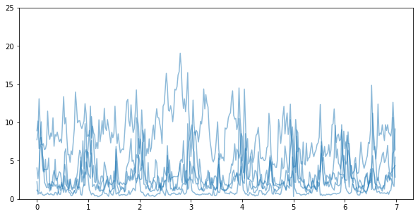
(a) 5 true consumption curves.

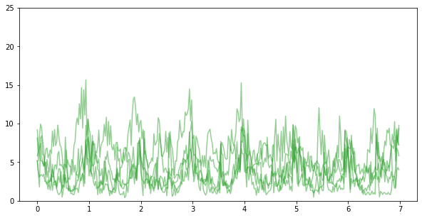
(b) 5 samples from the unbiased model $p$.

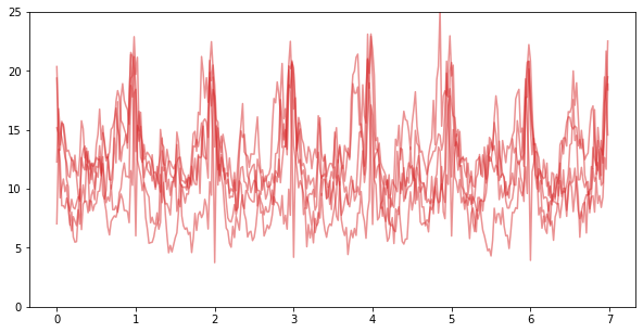
(c) 5 samples from the model $q_{\beta}$ tuned to maximize peak consumption.

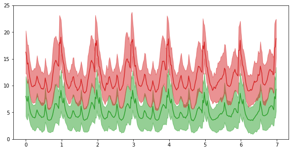
(d) Mean and standard deviation of samples generated after $p$ and $q_{\beta}$ tuned to maximize peak consumption.

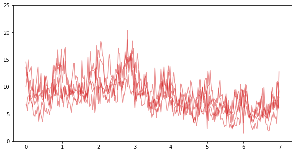
(e) 5 samples from the tuned model $q_{\beta}$ tuned to maximize Wednesday’s consumption only.

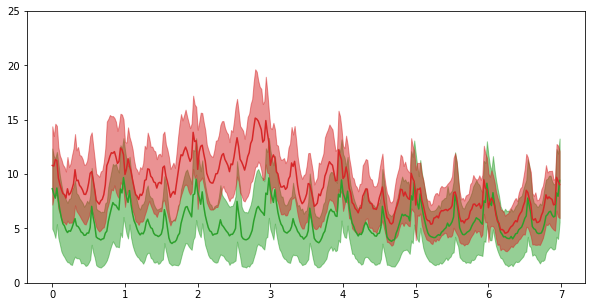
(f) Mean and standard deviation of samples generated after $p$ and $q_{\beta}$ tuned to maximize Wednesday’s consumption only.

Figure 2: Applying BTGM to tune the generation of weekly energy consumption curves, reporting the consumption (in kW on $y$ axis) vs the day (on $x$ axis).
Top: real sample curves (a) and $p$-generated samples, with $p$ the initial VAE model (b).
Middle row: tuning $p$ toward top 1% weekly energy consumption curves (criterion$f_{1}$); tuned generated samples (c), and comparison of $p$ with $p$ tuned after $f_{1}$ (d).
Bottom row: tuning $p$ toward top 1% Wednesday energy consumption curves (criterion$f_{2}$, see text); tuned generated samples (e), and comparison of $p$ with $p$ tuned after $f_{2}$ (f). The VAE $p$, composed of encoder and decoder modules with 10 blocks of residual networks each, is trained from ca 8 million weekly consumption curves; the mean and deviation of the initial and tuned generative models are computed over 1,000 samples. Better seen in color.

4.4 Refining a generative model a posteriori

Another potential usage of BTGM is to refine existing generative models, e.g. preventing a VAE from generating out-of-distribution samples (Arjovsky and Bottou, 2017). Let $p_{VAE}$ denote an overly general generative model, and let $f$ be defined as a adversarial classifier, discriminating the generated samples from the true data distribution $p_{D}$. When converged and in the large sample limit, the discriminator yields an estimation of $\frac{p_{D}(x)}{p_{D}(x)+p_{VAE}(x)}$ (Goodfellow et al., 2014).

When using criterion $f(x)=\log\frac{p_{D}(x)}{p_{VAE}(x)}$, given by the pre-activation output of the discriminator, to tune model $p_{VAE}$, one gets the generative model $q_{\beta}$ defined as:

$$q_{\beta}(x)\propto p_{VAE}(x)^{1-\beta}p_{D}(x)^{\beta}$$ (13)

In this scheme, BTGM aims to actually draw the generative model closer to the true distribution $p_{D}$. Compared to the mainstream GAN scheme, the difference is that the discriminator is used a posteriori: the generative modelling is decoupled from its adversarial tuning and the concurrent training procedure is replaced by the sequence of two (comparatively straightforward) optimization procedures, firstly training $p_{VAE}$ and secondly tuning it toward $f$. Results illustrating the proposed methodology are presented in Appendix F. This sequential adversarial generative modelling relies on two interdependent assumptions. Firstly, $p_{VAE}$ must be able to accurately reconstruct the whole training dataset; more precisely, the support of distribution $p_{VAE}$ must cover that of the data distribution $p_{D}$. Secondly, the discriminator needs be not saturated and give highly-confident predictions, for its gradient to provide sufficient information to refine $p_{VAE}$ (this also requires the former assumption to hold).

5 Discussion and Perspectives

The contribution of the paper is a new theoretical formulation and algorithm for the a posteriori refinement of a wide class of generative models, including GANs, VAEs, and explicit likelihood models. When the considered generative model relies on the use of a latent space, BTGM can operate directly in the latent space, favoring the scalability of the approach w.r.t. high-dimensional spaces. BTGM offers a new alternative to rejection sampling in order to explore the extreme quantiles of the data distribution w.r.t. any criterion $f$, subject to $f$ being differentiable. The proof of concept presented in the domain of energy management, where the consumption peak is estimated from the extreme quantiles of the consumption curves, is to our best knowledge the first and only alternative to rejection sampling in this context.

Three perspectives for further work are considered. In the short term, a first goal is to use BTGM to better understand when and why the dropping phenomenon occurs in the adversarial setting. On-going results show that a VAE model can indeed be refined a posteriori using a discriminator as criterion$f$; however, it is observed that mode dropping does appear when the pressure on $f$ is increased beyond a certain level. In order to avoid this loss of diversity, a research perspective is to extend BTGM to the general multi-criteria optimization setting, tuning the considered generative models with several criteria (e.g. the discriminator $f$, and the lequi-distribution of the classes).

A second perspective is to use BTGM in the context of privacy-sensitive data. The use of generative models for releasing non-sensitive though realistic samples has been explored (Torkzadehmahani et al., 2019; Long et al., 2019; Augenstein et al., 2020). BTGM makes it feasible to train a model from large datasets (thus offering a better model with better privacy guarantees) and focus it a posteriori on the target of interest, e.g. a rare mode of a disease. The eventual biased generative model will expectedly both inherit the privacy guarantees of the general model, and yield the focused samples as desired.

Another perspective is to extend BTGM in the direction of Bayesian Optimization (Mockus et al., 1978; Rasmussen, 2004), and Interactive Preference Learning pioneered by (Brochu et al., 2010; Viappiani and Boutilier, 2011). Specifically in the context of Optimal Design, the expert-in-the-loop setting can be leveraged to alternatively bias the generative model toward the experts’ preferences, and learn a model of their preferences. While facing the challenges of interactive preference learning, this approach would pave the way toward a focused augmentation of the data, under the experts’ control.

Appendix A Closed form derivatives of $D_{KL}(q\|p)$ and $\mathbb{E}_{q}f$

From Eqs. (1-2)

$$q_{\beta}(x)=\arg\min\int_{\mathcal{X}}q(x)f(x)dx+\frac{1}{\beta}\int_{\mathcal{X}}q(x)\log\frac{q(x)}{p(x)}dx$$

it follows:

$$q_{\beta}(x)=\frac{1}{Z(\beta)}p(x)e^{\beta f(x)}$$ (14)

with normalization constant $Z(\beta)$ ensuring that $q_{\beta}$ is a probability distribution. The derivatives of $D_{KL}(q\|p)$ and $\mathbb{E}_{q}f$ follow from Lemmas 1 and 2.

Lemma 1.

The derivative $\frac{d}{d\beta}\log Z(\beta)$ reads:

$${\frac{d}{d\beta}\log Z(\beta)=\mathbb{E}_{q_{\beta}}f}$$ (15)

Proof.

As $Z(\beta)=\int_{x}p(x)e^{\beta f(x)}dx$ by definition, it follows:

$$\frac{d}{d\beta}\log Z(\beta) =\frac{1}{Z(\beta)}\frac{d}{d\beta}Z(\beta)$$ (16)

$$=\frac{1}{Z(\beta)}\frac{d}{d\beta}\int_{\cal X}p(x)e^{\beta f(x)}dx$$

$$=\frac{1}{Z(\beta)}\int_{\cal X}f(x)p(x)e^{\beta f(x)}dx$$

$$=\int_{x}f(x)q_{\beta}(x)$$

$$=\mathbb{E}_{q_{\beta}}f$$

∎

Lemma 2.

Let $h:\mathcal{X}\rightarrow\mathbb{R}$ be a function (possibly depending on $\beta$). The derivative of its expectation on $q_{\beta}$ wrt $\beta$ reads:

$${\frac{d}{d\beta}\mathbb{E}_{q_{\beta}}h=\mathbb{E}_{q\beta}\left[fh+\frac{\partial h}{\partial\beta}\right]-\left(\mathbb{E}_{q_{\beta}}f\right)\left(\mathbb{E}_{q_{\beta}}h\right)}$$ (17)

Proof.

$$\frac{d}{d\beta}\mathbb{E}_{q_{\beta}}h =\frac{d}{d\beta}\frac{1}{Z(\beta)}\int_{x}h(x)p(x)e^{\beta f(x)}dx$$ (18)

$$=\frac{1}{Z(\beta)}\int_{x}\left(h(x)f(x)+\frac{\partial h}{\partial\beta}(x)\right)p(x)e^{\beta f(x)}dx$$

$$\quad-\frac{1}{Z(\beta)^{2}}\frac{dZ}{d\beta}\int_{x}h(x)p(x)e^{\beta f(x)}dx$$

$$=\mathbb{E}_{q_{\beta}}\left[hf+\frac{\partial h}{\partial\beta}\right]-\left(\mathbb{E}_{q_{\beta}}h\right)\frac{d}{d\beta}\log Z(\beta)$$

$$=\mathbb{E}_{q\beta}\left[fh+\frac{\partial h}{\partial\beta}\right]-\left(\mathbb{E}_{q_{\beta}}f\right)\left(\mathbb{E}_{q_{\beta}}h\right)$$

∎

Lemmas 1 and 2 yield the first and second derivatives of $\mathbb{E}_{q_{\beta}}f$.

Lemma 3.

The first and second derivatives of $\mathbb{E}_{q_{\beta}}f$ wrt $\beta$ read:

$${\frac{d}{d\beta}\mathbb{E}_{q_{\beta}}f=Var_{q_{\beta}}f}\quad\text{and}\quad{\frac{d^{2}}{d\beta^{2}}\mathbb{E}_{q_{\beta}}f=\mathbb{E}_{q_{\beta}}\left(f-\mathbb{E}_{q_{\beta}}f\right)^{3}}$$ (19)

Proof.

Replacing $h$ with $f$ in Eq. 17, and noting that $f$ does not depend on $\beta$, yields the first derivative:

$$\frac{d}{d\beta}\mathbb{E}_{q_{\beta}}f=\mathbb{E}_{q_{\beta}}f^{2}-\left(\mathbb{E}_{q_{\beta}}f\right)^{2}=Var_{q_{\beta}}f$$ (20)

Noting that $Var_{q_{\beta}}f=\mathbb{E}_{q_{\beta}}\left(f-\mathbb{E}_{q_{\beta}}f\right)^{2}$ and replacing $h$ with $\left(f-\mathbb{E}_{q_{\beta}}f\right)^{2}$ (that does depend on $\beta$) in Eq. 17 yields the second derivative:

$$\frac{d^{2}}{d\beta^{2}}\mathbb{E}_{q_{\beta}}f =\frac{d}{d\beta}\mathbb{E}_{q_{\beta}}\left(f-\mathbb{E}_{q_{\beta}}f\right)^{2}$$ (21)

$$=\mathbb{E}_{q_{\beta}}\left[f\left(f-\mathbb{E}_{q_{\beta}}f\right)^{2}-2\left(f-\mathbb{E}_{q_{\beta}}f\right)\frac{d}{d\beta}\mathbb{E}_{q_{\beta}}f\right]-\left(\mathbb{E}_{q_{\beta}}f\right)\left(\mathbb{E}_{q_{\beta}}\left(f-\mathbb{E}_{q_{\beta}}f\right)^{2}\right)$$

$$=\mathbb{E}_{q_{\beta}}\left(f-\mathbb{E}_{q_{\beta}}f\right)^{3}-2\underbrace{\mathbb{E}_{q_{\beta}}\left[f-\mathbb{E}_{q_{\beta}}f\right]}_{=0}\frac{d}{d\beta}\mathbb{E}_{q_{\beta}}f$$

$$=\mathbb{E}_{q_{\beta}}\left(f-\mathbb{E}_{q_{\beta}}f\right)^{3}$$

∎

Lemmas 1 and 2 likewise yield the first and second derivatives of $D_{KL}(q_{\beta}\|p)$:

Lemma 4.

The first and second derivatives of $\mathbb{E}_{q_{\beta}}f$ wrt $\beta$ read:

$${\frac{d}{d\beta}D_{KL}(q_{\beta}\|p)=\beta Var_{q_{\beta}}f}\quad\text{and}\quad{\frac{d^{2}}{d\beta^{2}}D_{KL}(q_{\beta}\|p)=Var_{q_{\beta}}f+\beta\mathbb{E}_{q_{\beta}}\left(f-\mathbb{E}_{q_{\beta}}f\right)^{3}}$$ (22)

Proof.

By definition:

$$D_{KL}(q_{\beta}\|p) =\mathbb{E}_{q_{\beta}}\log\frac{q_{\beta}}{p}$$ (23)

$$=\mathbb{E}_{q_{\beta}}\left[\beta f-\log Z(\beta)\right]$$

$$=\beta\mathbb{E}_{q_{\beta}}\left[f\right]-\log Z(\beta)$$

Lemmas 1 and 2 thus yield:

$$\frac{d}{d\beta}D_{KL}(q_{\beta}\|p) =\mathbb{E}_{q_{\beta}}\left[f\right]+\beta\frac{d}{d\beta}\mathbb{E}_{q_{\beta}}\left[f\right]-\frac{d}{d\beta}\log Z(\beta)$$ (24)

$$=\mathbb{E}_{q_{\beta}}\left[f\right]+\beta Var_{q_{\beta}}\left[f\right]-\mathbb{E}_{q_{\beta}}\left[f\right]$$

$$=\beta Var_{q_{\beta}}f$$

and:

$$\frac{d}{d\beta}D_{KL}(q_{\beta}\|p) =Var_{q_{\beta}}f+\beta\frac{d}{d\beta}Var_{q_{\beta}}f$$ (25)

$$=Var_{q_{\beta}}f+\beta\mathbb{E}_{q_{\beta}}\left(f-\mathbb{E}_{q_{\beta}}f\right)^{3}$$

which concludes the proof. ∎

Appendix B Bounding $KL(q\|p)$ on latent space

Lemma 5.

Let $p(x,z)$ be a generative model built on a sampling of a latent space ($p(x,z)=p(z)p(x|z)$, with $p(x|z)$ the decoder mapping the latent onto the instance space). Let generative model $q(x,z)$ be defined as $q(x,z)=q(z)p(x|z)$ (freezing the decoder and modifying the latent distribution). Then:

$${D_{KL}(q(x)\|p(x))\leq D_{KL}(q(z)\|p(z))}$$ (26)

Proof.

It is seen that, for any two distributions $q$ and $p$ of two variables, the Kullback-Leibler divergence between their marginals is always smaller than the Kullback-Leibler divergence between the full distributions:

$$D_{KL}(q(a,b)\|p(a,b)) =\mathbb{E}_{q}\log\frac{q(a,b)}{p(a,b)}$$ (27)

$$=\mathbb{E}_{q}\log\frac{q(a)q(b|a)}{p(a)p(b|a)}$$

$$=D_{KL}(q(a)\|p(a))+\mathbb{E}_{q}D_{KL}(q(b|a)\|p(b|a))$$

$$\geq D_{KL}(q(a)\|p(a))$$

Replacing $p(a,b)$ with $p(x,z)=p(z)p(x|z)$ (respectively, $q(a,b)$ with $q(x,z)=q(z)p(x|z)$) yields:

$$D_{KL}(q(x)\|p(x)) \leq D_{KL}(q(x,z)\|p(x,z))$$ (28)

$$\leq D_{KL}(q(z)\|p(z))+\mathbb{E}_{q}\underbrace{D_{KL}(p(x|z)\|p(x|z))}_{=0}$$

$$\leq D_{KL}(q(z)\|p(z))$$

∎

Appendix C Comparing two criteria: detailed analysis

As the intended bias can be expressed using different criteria, the question of comparing these (based on the distribution of their gradient norms) was discussed in section 4.2. Complementary experiments are conducted as follows, along the same setting aimed to conditionalize generative model $p$ using a classifier $p(\ell|x)$.

A first remark is that the closed form values of $\mathbb{E}_{q_{\beta}}f$ and $D_{KL}(q_{\beta}\|p)$ can be estimated using samples from $p$. Specifically, expectations under $q_{\beta}$ can be reframed as expectations under $p$:

$$Z(\beta)=\int_{\mathcal{X}}p(x)e^{\beta f(x)}dx=\mathbb{E}_{p}\left[e^{\beta f}\right]$$ (29)

$$\mathbb{E}_{q_{\beta}}f=\int_{\mathcal{X}}f(x)\frac{p(x)e^{\beta f(x)}}{Z(\beta)}dx=\frac{\mathbb{E}_{p}\left[fe^{\beta f}\right]}{\mathbb{E}_{p}\left[e^{\beta f}\right]}$$ (30)

$$D_{KL}(q_{\beta}\|p)=\beta\mathbb{E}_{q_{\beta}}\left[f\right]-\log Z(\beta)=\frac{\mathbb{E}_{p}\left[fe^{\beta f}\right]}{\mathbb{E}_{p}\left[e^{\beta f}\right]}-\log\mathbb{E}_{p}\left[e^{\beta f}\right]$$ (31)

Eqs. 30-31 enable to estimate the closed form values of $\mathbb{E}_{q_{\beta}}f$ and $D_{KL}(q_{\beta}\|p)$ vs $\beta$, using samples drawn after $p$. The comparison of these estimates with the actual $\mathbb{E}_{\hat{q}_{\beta}}f$ and $D_{KL}(\hat{q}_{\beta}\|p)$ indicates how well BTGM is dealing with the considered criterion.

In the considered example, one wants to compare both criteria $f_{h}$ and $f_{\log h}$, respectively defined as $f_{h}(x)=p(\ell|x)$ and $f_{\log h}(x)=logp(\ell|x)$. The discrepancy between the theoretical estimate and the actual estimate is displayed on Fig. 3 for $f_{h}$ (respectively Fig. 4 for $f_{\log h}$). The same optimization procedure was used in both cases, targeting the class $\ell=4$.

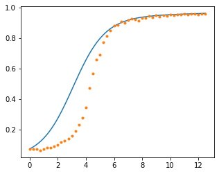
(a) $\mathbb{E}_{q_{\beta}}\,f_{h}$ ($y$ axis) vs $\beta$ ($x$ axis).

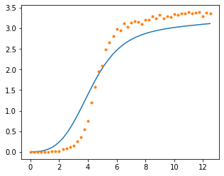
(b) $D_{KL}(q_{\beta}\|p)$ ($y$ axis) vs $\beta$ ($x$ axis).

(c) $\mathbb{E}_{q_{\beta}}\,f_{h}$ ($y$ axis) vs $D_{KL}(q_{\beta}\|p)$ ($x$ axis).

Figure 3: Theoretical (plain line) and experimental (dashed line) estimates of $\mathbb{E}_{q_{\beta}}\,f_{h}$ and $D_{KL}(q_{\beta}\|p)$ vs $\beta$ for $f(x)=h(\ell=4|x)$.

(a) $\mathbb{E}_{q_{\beta}}\,f_{\log h}$ ($y$ axis) vs $\beta$ ($x$ axis).

(b) $D_{KL}(q_{\beta}\|p)$ ($y$ axis) vs $\beta$ ($x$ axis).

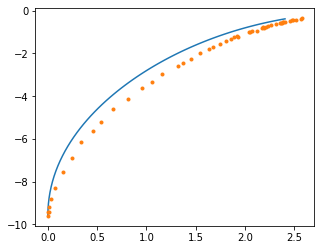
(c) $\mathbb{E}_{q_{\beta}}\,f_{\log h}$ ($y$ axis) vs $D_{KL}(q_{\beta}\|p)$ ($x$ axis).

Figure 4: Theoretical (plain line) and experimental (dashed line) estimates of $\mathbb{E}_{q_{\beta}}\,f_{\log h}$ and $D_{KL}(q_{\beta}\|p)$ vs $\beta$ for $f(x)=\log h(\ell=4|x)$.

For small values of $\beta$, with criterion $f_{h}$, Fig. 3 shows that the empirical $\mathbb{E}_{q_{\beta}}\,f_{h}$ does not much increase, while $q_{\beta}$ remains close to $p$ ($D_{KL}(q_{\beta}\|p)$ stays close to 0). In other words, the bias seems ineffective. Quite the contrary, for large values of $\beta$, the empirical $D_{KL}(q_{\beta}\|p)$ increases significantly faster than the theoretical estimate; BTGM overshoots and focuses too much the support of distribution $q_{\beta}$. In comparison, a much smaller gap between the theoretical and empirical estimates is observed with criterion $f_{log.h}$ (Fig. 4).

These observations are in agreement with the analysis proposed in section 4.2: $f_{h}$ only provides useful gradients in the boundary of the targeted class. Accordingly, the process finds itself in one out of two stable states: doing nothing ($q_{\beta}=p$); or restricting the support of $q_{\beta}$ to that of the targeted class. BTGM abruptly switches from the first to the second stable state (Fig. 3.b), offering little control through $\beta$. When setting $f(x)=\log p(\ell|x))$ instead, $f(x)$ is less and less often saturated, enabling its gradient to provide smooth information. This information enables the user to finely control the bias through $\beta$, making the support of $q_{\beta}$ to gracefully tend toward the support of the targeted class.

Appendix D Generality of the approach: a proof of concept on MNIST

The claim is that BTGM can be applied using any differentiable criterion (with exploitable gradient, see Appendix C. above). Three criteria are illustrated on Figs. 5, 6 and 7, respectively biasing the generative process toward a certain class, figures with more white pixels, or less white pixels.

The fine-grained control of the bias is illustrated on Fig. 5 on MNIST, with target class $\ell=4$, using a GAN model $p$. The Pareto front depicting the bi-criteria optimization trade-off ($\mathbb{E}_{q_{\beta}}f$ vs $D_{KL}(q_{\beta}\|\ p)$ for $\beta$ ranging from 0 to 2.5) is displayed on Fig. 5(a), and the biased generated samples, where each row from top to bottom displays the samples generated with increasing values of $\beta$, are displayed on Fig. 5(b). Indeed, class 4 is more prevalent as $\beta$ increases; class 9 is the last one to disappear, as being the most similar to the 4 one; for the highest values of $\beta$, only digits in class 4 are generated, yielding the same result as a conditional generative model, as expected.

A similar interpretation can be made for the two other examples on Figs. 6 and 7.

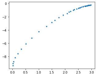
(a) $\mathbb{E}_{q_{\beta}}\,f$ ($y$ axis) vs $D_{KL}(q_{\beta}\|p)$ ($x$ axis).

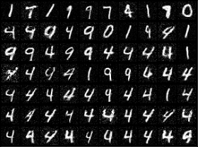
(b) Generated samples, with the strength $\beta$ of the bias increasing from top to bottom rows.

Figure 5: Using BTGM to condition a generative model in the latent space, with $p$ a GAN trained on MNIST and $f=\log{\hat{h}(\text{class }4\,|\,z)}$, and $h$ an independently trained classifier on the instance space. Left: Pareto front of both criteria. Right: generated samples, with top to bottom rows respectively corresponding to $\beta$ in $\{0.0,0.25,0.5,0.75,1.0,1.25\}$, and corresponding $D_{KL}$ values $0.0,0.4,1.3,2.2,2.5,2.7$.

(a) $\mathbb{E}_{q_{\beta}}\,f$ ($y$ axis) vs $D_{KL}(q_{\beta}\|p)$ ($x$ axis).

(b) Generated samples, with the strength $\beta$ of the bias increasing from top to bottom rows.

Figure 6: Using BTGM to condition a generative model in the latent space, with $p$ a GAN trained on MNIST and $f(x)=\sum_{i\in pixels}x_{i}$. Left: Pareto front of both criteria. Right: generated samples, with top to bottom rows respectively corresponding to $\beta$ in $\{0.0,0.025,0.05,0.075,0.1,0.125,0.150\}$, and corresponding $D_{KL}$ values $0.0,0.3,2.1,3.9,5.4,7.4,8.7$.

(a) $\mathbb{E}_{q_{\beta}}\,f$ ($y$ axis) vs $D_{KL}(q_{\beta}\|p)$ ($x$ axis).

(b) Generated samples, with the strength $\beta$ of the bias increasing from top to bottom rows.

Figure 7: Using BTGM to condition a generative model in the latent space, with $p$ a GAN trained on MNIST and $f(x)=\sum_{i\in pixels}x_{i}$. Left: Pareto front of both criteria. Right: generated samples, with top to bottom rows respectively corresponding to $\beta$ in $\{0.0,0.025,0.05,0.075,0.1,0.125,0.150\}$, and corresponding $D_{KL}$ values $0.0,0.2,0.6,1.1,1.4,1.8,2.1$.

As seen on Fig. 6, biasing the generative model toward figures with more white pixels is achieved through controlling both the class of the generated figures (class $0$ and $8$) and the style of the generated numbers (with thick strokes). Quite the contrary, biasing the generative model toward figures with less white pixels results in generating very thin 1s.

Appendix E Rejection sampling with BTGM in a real-world application

As said, the application domain concerns smart grid management and dimensioning. The latter requires key indicators (consumption peak) to be estimated from consumption curves generated under diverse scenarii. A versatile generative model is trained with a VAE, exploiting real weekly consumption curves aggregated over 10 households (thus with a higher variance compared to the curves aggregated over 100 households, considered in the main paper).

The flexibility of the approach is demonstrated using several criteria.

The first criterion aims to maximize the consumption over a particular day (here Wednesday, Fig. 8(a)). The goal is achieved by maximizing the weekly consumption, with the consumption on Wednesday being only slightly higher than the average one. The second criterion aims to maximize the difference between the Wednesday consumption and the average weekly consumption (intuitively, this criterion corresponds to a worst-case analysis scenario). Using this criterion and allowing the $D_{KL}$ to take large values (corresponding to a rejection sampling with probability $10^{-4}$) yields the curves illustrated on Fig. 8(b). Despite the strength of the bias, BTGM still manages to generate diverse samples; furthermore, the sample variance is comparable to that of the original data.

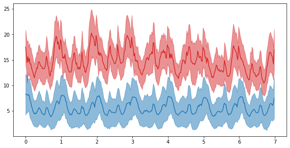
(a) Maximizing the consumption of Wednesday.

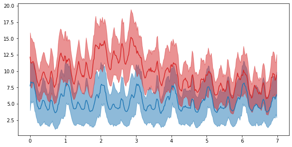
(b) Maximizing the difference between the consumption of Wednesday and the average weekly consumption.

Figure 8: Application of BTGM in the context of energy management: generating consumption curves biased according to: Average Wednesday consumption (8(a)); Average Wednesday consumption and difference between Wednesday consumption and average weekly consumption (8(b)). Blue curves represent the mean and standard deviation of samples from the original model, and red curves that of samples from the biased model (best seen in color).

The third criterion is related to the variability of the demand, with a high impact on the required flexibility of electricity production. A relevant indicator, referred to as MAE by abuse of the definition, is the amount of consumption that would need to be moved in order to make the consumption constant along time (with same overall consumption), i.e. the L1 distance between the actual consumption curve and the flat curve with same overall consumption. Fig. 9 displays average generated consumption curves when applying BTGM to maximize or minimize the MAE.

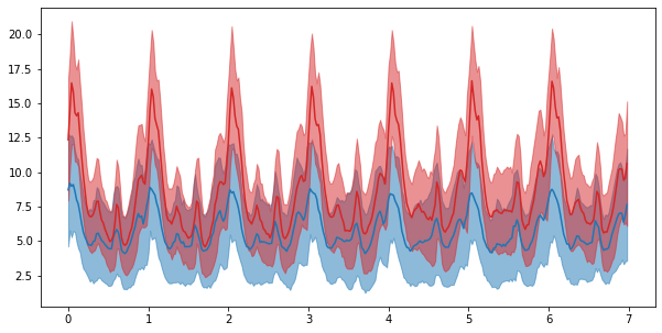
(a) Maximizing the L1 distance to mean consumption.

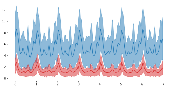
(b) Minimizing the L1 distance to mean consumption.

Figure 9: Application of BTGM in the context of energy management: generating consumption curves biased to maximize (9(a)) and minimize (9(b)) the L1 distance between the consumption and its average. Blue curves represent the mean and standard deviation of samples from the original model, and red curves that of samples from the biased model (best seen in color).

The curves obtained when minimizing the MAE (Fig. 9(b)) can be interpreted intuitively as: a good way to get a flat consumption curve is when the house is empty (e.g. during holidays), since inhabited houses typically present strong cyclical patterns across the day.

When maximizing the MAE (Fig. 9(a)), the interpretation of the obtained curves is equally straightforward: BTGM takes advantage of the natural variability of the data to significantly increase the height of the consumption peaks, while only slightly increasing the average consumption, thereby yielding a high variance of the daily consumption.

Appendix F Adversarially refining a generative model using BTGM: Discussion

A possible usage of BTGM is to focus an overly general generative model (with support covering the data support) along an adversarial scheme, using a discriminator trained to distinguish between the actual and the generated samples as criterion $f$.

Experiments are conducted to examine the feasibility of this 2-step generative modelling approach, with $p$ a VAE trained on MNIST and $g$ a classifier trained to discriminate the actual and the generated data (with accuracy $0.99$), using its pre-activation output as $f$. BTGM is applied on the VAE’s latent space, and results are displayed on Fig. 10.

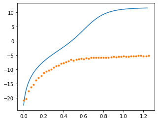
(a) $\mathbb{E}_{q_{\beta}}\,f$ ($y$ axis) vs $\beta$ ($x$ axis).

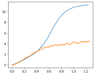
(b) $D_{KL}(q_{\beta}\|p)$ ($y$ axis) vs $\beta$ ($x$ axis).

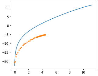
(c) $\mathbb{E}_{q_{\beta}}\,f$ ($y$ axis) vs $D_{KL}(q_{\beta}\|p)$ ($x$ axis).

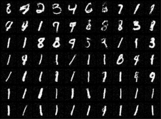
(d) Generated samples, with the strength $\beta$ of the bias increasing from top to bottom rows.

Figure 10: BTGM: adversarial refinement of $p$ (VAE trained on MNIST) along criterion $f$, with $f$ a discriminator. As in Appendix C, Blue line are the theoretical curves, and orange dots are the empirical values. 10(a), 10(b): Evolution of $\mathbb{E}_{q_{\beta}}\,f$ and $D_{KL}(q_{\beta}\|p)$ with $\beta$ . 10(c): Pareto front of both criteria. 10(d): generated samples with a clear mode dropping phenomenon, with top to bottom rows respectively corresponding to $\beta$ in $\{0.0,0.125,0.250,0.375,0.5,0.625,0.750\}$ and corresponding $D_{KL}$ values $0.0,0.6,1.4,2.4,2.9,3.6,3.7$.

With same methodology as in Appendix C, the optimization process is assessed by comparing the theoretical and the empirical estimates of $\mathbb{E}_{q_{\beta}}\,f$ and $D_{KL}(q_{\beta}\|p)$.

The optimization fails: for $\beta\geq 0.5$, the $D_{KL}$ stagnates, that is, BTGM cannot push $q_{\beta}$ farther away from $p$. For $\beta<0.5$, BTGM does not manage to increase $\mathbb{E}_{q_{\beta}}\,f$ as expected from the theoretical estimate.

This change of behavior around $\beta=.5$ is analyzed in relation with the distribution of $f$ gradients wrt to $p$ (Fig. 11), involving most gradient norms in a reasonable range ($[0;10]$), while some gradients do explode with a norm as large as 230. This suggests that the optimization landscape includes large smooth regions with some very sharp regions (cliffs).

It is noted that at the change point ($\beta\approx.5$), $D_{KL}\approx 4$, that is, $q_{\beta}$ is focused on approximately 2% of the support of $p$. Our interpretation is that, at this point the process meets the high gradient norm region and remains stuck.

The fact that BTGM cannot thus refine $p$ using the adversarial criterion is eventually blamed on two factors. Firstly, the discriminator seems sufficiently powerful to characterize the support of the true data as a set of isolated regions separated by high cliffs. Secondly, the generative model search space (based on Normalizing Flows; specifically, 6 Inverse AutoRegressive flows layers, each consisting of 4 fully-connected layers) seems not flexible enough to comply with the discriminator, and to approximate a mixture. Eventually, BTGM is unable to modify the structure of $p$ as desired in the small $\beta$ region (with $\mathbb{E}_{q_{\beta}}\,f$ about twice smaller than the theoretical estimate); and totally unable to modify it for $\beta>.5)$. How to remedy both limitations is left for future work.

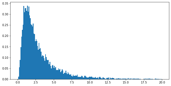
Figure 11: Distribution of the norm of the gradient of the objective $f$ (pre-activation output of the discriminator) wrt to the latent variable. The histogram is truncated at a norm of $20$ for legibility, but around $1\%$ of the gradients have a higher norm, going up to $230$.

References

- Alemi et al. (2018) A. Alemi, B. Poole, I. Fischer, J. Dillon, R. A. Saurous, and K. Murphy. Fixing a Broken ELBO. In International Conference on Machine Learning, pages 159–168, July 2018. ISSN: 1938-7228 Section: Machine Learning.
- Ardizzone et al. (2019) L. Ardizzone, J. Kruse, S. Wirkert, D. Rahner, E. W. Pellegrini, R. S. Klessen, L. Maier-Hein, C. Rother, and U. Köthe. Analyzing Inverse Problems with Invertible Neural Networks. ICLR 2019, Feb. 2019. arXiv: 1808.04730.
- Arjovsky and Bottou (2017) M. Arjovsky and L. Bottou. Towards Principled Methods for Training Generative Adversarial Networks. arXiv:1701.04862 [cs, stat], Jan. 2017. arXiv: 1701.04862.
- Arjovsky et al. (2017) M. Arjovsky, S. Chintala, and L. Bottou. Wasserstein Generative Adversarial Networks. In International Conference on Machine Learning, pages 214–223, July 2017. ISSN: 1938-7228 Section: Machine Learning.
- Augenstein et al. (2020) S. Augenstein, H. B. McMahan, D. Ramage, S. Ramaswamy, P. Kairouz, M. Chen, R. Mathews, and B. A. y. Arcas. Generative Models for Effective ML on Private, Decentralized Datasets. ICLR 2020, Feb. 2020. arXiv: 1911.06679.
- Bessiere et al. (2017) C. Bessiere, F. Koriche, N. Lazaar, and B. O’Sullivan. Constraint acquisition. Artificial Intelligence, 244:315–342, Mar. 2017. ISSN 0004-3702. doi: 10.1016/j.artint.2015.08.001.
- Bishop et al. (1998) C. M. Bishop, N. D. Lawrence, T. Jaakkola, and M. I. Jordan. Approximating Posterior Distributions in Belief Networks Using Mixtures. In M. I. Jordan, M. J. Kearns, and S. A. Solla, editors, Advances in Neural Information Processing Systems 10, pages 416–422. MIT Press, 1998.
- Boyd and Vandenberghe (2004) S. P. Boyd and L. Vandenberghe. Convex Optimization. Cambridge University Press, Mar. 2004. ISBN 978-0-521-83378-3.
- Brochu et al. (2010) E. Brochu, V. M. Cora, and N. de Freitas. A Tutorial on Bayesian Optimization of Expensive Cost Functions, with Application to Active User Modeling and Hierarchical Reinforcement Learning. arXiv:1012.2599 [cs], Dec. 2010. arXiv: 1012.2599.
- Burda et al. (2016) Y. Burda, R. Grosse, and R. Salakhutdinov. Importance Weighted Autoencoders. arXiv:1509.00519 [cs, stat], Nov. 2016. arXiv: 1509.00519.
- Chen et al. (2020) J. Chen, C. Lu, B. Chenli, J. Zhu, and T. Tian. VFlow: More Expressive Generative Flows with Variational Data Augmentation. arXiv:2002.09741 [cs, stat], July 2020. arXiv: 2002.09741.
- Choi et al. (2019) H. Choi, E. Jang, and A. A. Alemi. WAIC, but Why? Generative Ensembles for Robust Anomaly Detection. arXiv:1810.01392 [cs, stat], May 2019. arXiv: 1810.01392 version: 4.
- Chu et al. (2017) C. Chu, A. Zhmoginov, and M. Sandler. CycleGAN, a Master of Steganography. 2017.
- Courty et al. (2017) N. Courty, R. Flamary, A. Habrard, and A. Rakotomamonjy. Joint distribution optimal transportation for domain adaptation. In I. Guyon, U. V. Luxburg, S. Bengio, H. Wallach, R. Fergus, S. Vishwanathan, and R. Garnett, editors, Advances in Neural Information Processing Systems 30, pages 3730–3739. Curran Associates, Inc., 2017.
- Dash et al. (2020) S. Dash, A. Yale, I. Guyon, and K. P. Bennett. Medical Time-Series Data Generation Using Generative Adversarial Networks. In M. Michalowski and R. Moskovitch, editors, Artificial Intelligence in Medicine, Lecture Notes in Computer Science, pages 382–391, Cham, 2020. Springer International Publishing. ISBN 978-3-030-59137-3. doi: 10.1007/978-3-030-59137-3_34.
- Dinh et al. (2015) L. Dinh, D. Krueger, and Y. Bengio. NICE: Non-linear Independent Components Estimation. arXiv:1410.8516 [cs], Apr. 2015. arXiv: 1410.8516.
- Dinh et al. (2017) L. Dinh, J. Sohl-Dickstein, and S. Bengio. Density estimation using Real NVP. ICLR 2017, Feb. 2017. arXiv: 1605.08803.
- Ganin et al. (2016) Y. Ganin, E. Ustinova, H. Ajakan, P. Germain, H. Larochelle, F. Laviolette, M. March, and V. Lempitsky. Domain-Adversarial Training of Neural Networks. Journal of Machine Learning Research, 17(59):1–35, 2016.
- Gershman et al. (2012) S. J. Gershman, M. D. Hoffman, and D. M. Blei. Nonparametric variational inference. In Proceedings of the 29th International Coference on International Conference on Machine Learning, ICML’12, pages 235–242, Edinburgh, Scotland, June 2012. Omnipress. ISBN 978-1-4503-1285-1.
- Gonen (2015) T. Gonen. Electrical Power Transmission System Engineering: Analysis and Design, Third Edition. CRC Press, Aug. 2015. ISBN 978-1-4822-3223-3. Google-Books-ID: 6KbNBQAAQBAJ.
- Goodfellow et al. (2014) I. Goodfellow, J. Pouget-Abadie, M. Mirza, B. Xu, D. Warde-Farley, S. Ozair, A. Courville, and Y. Bengio. Generative Adversarial Nets. In Z. Ghahramani, M. Welling, C. Cortes, N. D. Lawrence, and K. Q. Weinberger, editors, Advances in Neural Information Processing Systems 27, pages 2672–2680. Curran Associates, Inc., 2014.
- Guo et al. (2017) F. Guo, X. Wang, K. Fan, T. Broderick, and D. B. Dunson. Boosting Variational Inference. arXiv:1611.05559 [cs, stat], Mar. 2017. arXiv: 1611.05559.
- Higgins et al. (2017) I. Higgins, L. Matthey, A. Pal, C. Burgess, X. Glorot, M. M. Botvinick, S. Mohamed, and A. Lerchner. beta-VAE: Learning Basic Visual Concepts with a Constrained Variational Framework. In ICLR, 2017.
- Hoffman et al. (2013) M. D. Hoffman, D. M. Blei, C. Wang, and J. Paisley. Stochastic variational inference. The Journal of Machine Learning Research, 14(1):1303–1347, May 2013. ISSN 1532-4435.
- Huang et al. (2019) C.-W. Huang, K. Sankaran, E. Dhekane, A. Lacoste, and A. Courville. Hierarchical Importance Weighted Autoencoders. In International Conference on Machine Learning, pages 2869–2878, May 2019. ISSN: 1938-7228 Section: Machine Learning.
- Jaiswal et al. (2019) A. Jaiswal, W. AbdAlmageed, Y. Wu, and P. Natarajan. Bidirectional Conditional Generative Adversarial Networks. In C. V. Jawahar, H. Li, G. Mori, and K. Schindler, editors, Computer Vision – ACCV 2018, Lecture Notes in Computer Science, pages 216–232, Cham, 2019. Springer International Publishing. ISBN 978-3-030-20893-6. doi: 10.1007/978-3-030-20893-6_14.
- Jang et al. (2017) E. Jang, S. Gu, and B. Poole. Categorical Reparameterization with Gumbel-Softmax. arXiv:1611.01144 [cs, stat], Aug. 2017. arXiv: 1611.01144.
- Kalatzis et al. (2020) D. Kalatzis, D. Eklund, G. Arvanitidis, and S. Hauberg. Variational Autoencoders with Riemannian Brownian Motion Priors. arXiv:2002.05227 [cs, stat], Feb. 2020. arXiv: 2002.05227.
- Kingma and Welling (2014) D. P. Kingma and M. Welling. Auto-Encoding Variational Bayes. arXiv:1312.6114 [cs, stat], May 2014. arXiv: 1312.6114.
- Kingma et al. (2014) D. P. Kingma, S. Mohamed, D. Jimenez Rezende, and M. Welling. Semi-supervised Learning with Deep Generative Models. In Z. Ghahramani, M. Welling, C. Cortes, N. D. Lawrence, and K. Q. Weinberger, editors, Advances in Neural Information Processing Systems 27, pages 3581–3589. Curran Associates, Inc., 2014.
- Kingma et al. (2017) D. P. Kingma, T. Salimans, R. Jozefowicz, X. Chen, I. Sutskever, and M. Welling. Improving Variational Inference with Inverse Autoregressive Flow. arXiv:1606.04934 [cs, stat], Jan. 2017. arXiv: 1606.04934.
- Ledig et al. (2017) C. Ledig, L. Theis, F. Huszar, J. Caballero, A. Cunningham, A. Acosta, A. Aitken, A. Tejani, J. Totz, Z. Wang, and W. Shi. Photo-Realistic Single Image Super-Resolution Using a Generative Adversarial Network. pages 4681–4690, 2017.
- Li et al. (2019) Y. Li, J. Bradshaw, and Y. Sharma. Are Generative Classifiers More Robust to Adversarial Attacks? In International Conference on Machine Learning, pages 3804–3814, May 2019. ISSN: 1938-7228 Section: Machine Learning.
- Long et al. (2019) Y. Long, S. Lin, Z. Yang, C. A. Gunter, and B. Li. Scalable Differentially Private Generative Student Model via PATE. arXiv:1906.09338 [cs, stat], June 2019. arXiv: 1906.09338.
- Mathieu et al. (2019a) E. Mathieu, C. Le Lan, C. J. Maddison, R. Tomioka, and Y. W. Teh. Continuous Hierarchical Representations with Poincaré Variational Auto-Encoders. In H. Wallach, H. Larochelle, A. Beygelzimer, F. d. Alché-Buc, E. Fox, and R. Garnett, editors, Advances in Neural Information Processing Systems 32, pages 12565–12576. Curran Associates, Inc., 2019a.
- Mathieu et al. (2019b) E. Mathieu, T. Rainforth, N. Siddharth, and Y. W. Teh. Disentangling Disentanglement in Variational Autoencoders. In International Conference on Machine Learning, pages 4402–4412, May 2019b. ISSN: 1938-7228 Section: Machine Learning.
- Mathieu et al. (2016) M. F. Mathieu, J. J. Zhao, J. Zhao, A. Ramesh, P. Sprechmann, and Y. LeCun. Disentangling factors of variation in deep representation using adversarial training. In D. D. Lee, M. Sugiyama, U. V. Luxburg, I. Guyon, and R. Garnett, editors, Advances in Neural Information Processing Systems 29, pages 5040–5048. Curran Associates, Inc., 2016.
- Miller et al. (2017) A. C. Miller, N. J. Foti, and R. P. Adams. Variational boosting: iteratively refining posterior approximations. In Proceedings of the 34th International Conference on Machine Learning - Volume 70, ICML’17, pages 2420–2429, Sydney, NSW, Australia, Aug. 2017. JMLR.org.
- Mirza and Osindero (2014) M. Mirza and S. Osindero. Conditional Generative Adversarial Nets. arXiv:1411.1784 [cs, stat], Nov. 2014. arXiv: 1411.1784.
- Mockus et al. (1978) J. Mockus, V. Tiesis, and A. Zilinskas. The application of Bayesian methods for seeking the extremum. Towards global optimization, 2(117-129):2, 1978.
- Nalisnick et al. (2019) E. Nalisnick, A. Matsukawa, Y. W. Teh, and B. Lakshminarayanan. Detecting Out-of-Distribution Inputs to Deep Generative Models Using Typicality. arXiv:1906.02994 [cs, stat], Oct. 2019. arXiv: 1906.02994.
- Nowozin et al. (2016) S. Nowozin, B. Cseke, and R. Tomioka. f-GAN: Training Generative Neural Samplers using Variational Divergence Minimization. In D. D. Lee, M. Sugiyama, U. V. Luxburg, I. Guyon, and R. Garnett, editors, Advances in Neural Information Processing Systems 29, pages 271–279. Curran Associates, Inc., 2016.
- Ong et al. (2018) V. M.-H. Ong, D. J. Nott, and M. S. Smith. Gaussian Variational Approximation With a Factor Covariance Structure. Journal of Computational and Graphical Statistics, 27(3):465–478, July 2018. ISSN 1061-8600. doi: 10.1080/10618600.2017.1390472. Publisher: Taylor & Francis _eprint: https://doi.org/10.1080/10618600.2017.1390472.
- Oord et al. (2016a) A. V. Oord, N. Kalchbrenner, and K. Kavukcuoglu. Pixel Recurrent Neural Networks. In International Conference on Machine Learning, pages 1747–1756, June 2016a. ISSN: 1938-7228 Section: Machine Learning.
- Oord et al. (2016b) A. v. d. Oord, S. Dieleman, H. Zen, K. Simonyan, O. Vinyals, A. Graves, N. Kalchbrenner, A. Senior, and K. Kavukcuoglu. WaveNet: A Generative Model for Raw Audio. arXiv:1609.03499 [cs], Sept. 2016b. arXiv: 1609.03499.
- Park et al. (2019) T. Park, M.-Y. Liu, T.-C. Wang, and J.-Y. Zhu. GauGAN: semantic image synthesis with spatially adaptive normalization. In ACM SIGGRAPH 2019 Real-Time Live!, SIGGRAPH ’19, page 1, Los Angeles, California, July 2019. Association for Computing Machinery. ISBN 978-1-4503-6315-0. doi: 10.1145/3306305.3332370.
- Pidhorskyi et al. (2018) S. Pidhorskyi, R. Almohsen, and G. Doretto. Generative Probabilistic Novelty Detection with Adversarial Autoencoders. In S. Bengio, H. Wallach, H. Larochelle, K. Grauman, N. Cesa-Bianchi, and R. Garnett, editors, Advances in Neural Information Processing Systems 31, pages 6822–6833. Curran Associates, Inc., 2018.
- Radford et al. (2016) A. Radford, L. Metz, and S. Chintala. Unsupervised Representation Learning with Deep Convolutional Generative Adversarial Networks. arXiv:1511.06434 [cs], Jan. 2016. arXiv: 1511.06434.
- Ranganath et al. (2014) R. Ranganath, S. Gerrish, and D. Blei. Black Box Variational Inference. In Artificial Intelligence and Statistics, pages 814–822, Apr. 2014. ISSN: 1938-7228 Section: Machine Learning.
- Rasmussen (2004) C. E. Rasmussen. Gaussian Processes in Machine Learning. In O. Bousquet, U. von Luxburg, and G. Rätsch, editors, Advanced Lectures on Machine Learning: ML Summer Schools 2003, Canberra, Australia, February 2 - 14, 2003, Tübingen, Germany, August 4 - 16, 2003, Revised Lectures, Lecture Notes in Computer Science, pages 63–71. Springer, Berlin, Heidelberg, 2004. ISBN 978-3-540-28650-9. doi: 10.1007/978-3-540-28650-9_4.
- Razavi et al. (2019) A. Razavi, A. van den Oord, and O. Vinyals. Generating Diverse High-Fidelity Images with VQ-VAE-2. In H. Wallach, H. Larochelle, A. Beygelzimer, F. d. Alché-Buc, E. Fox, and R. Garnett, editors, Advances in Neural Information Processing Systems 32, pages 14866–14876. Curran Associates, Inc., 2019.
- Rezende and Mohamed (2015) D. Rezende and S. Mohamed. Variational Inference with Normalizing Flows. In International Conference on Machine Learning, pages 1530–1538, June 2015. ISSN: 1938-7228 Section: Machine Learning.
- Rezende and Viola (2018) D. J. Rezende and F. Viola. Taming VAEs. arXiv:1810.00597 [cs, stat], Oct. 2018. arXiv: 1810.00597.
- Rezende et al. (2014) D. J. Rezende, S. Mohamed, and D. Wierstra. Stochastic Backpropagation and Approximate Inference in Deep Generative Models. In International Conference on Machine Learning, pages 1278–1286, Jan. 2014. ISSN: 1938-7228 Section: Machine Learning.
- Roberts et al. (2018) A. Roberts, J. Engel, C. Raffel, C. Hawthorne, and D. Eck. A Hierarchical Latent Vector Model for Learning Long-Term Structure in Music. In International Conference on Machine Learning, pages 4364–4373. PMLR, July 2018. ISSN: 2640-3498.
- Roy et al. (2018) A. Roy, A. Vaswani, A. Neelakantan, and N. Parmar. Theory and Experiments on Vector Quantized Autoencoders. arXiv:1805.11063 [cs, stat], July 2018. arXiv: 1805.11063.
- Sajjadi et al. (2018) M. S. M. Sajjadi, G. Parascandolo, A. Mehrjou, and B. Schölkopf. Tempered Adversarial Networks. In International Conference on Machine Learning, pages 4451–4459, July 2018. ISSN: 1938-7228 Section: Machine Learning.
- Salimans et al. (2017) T. Salimans, A. Karpathy, X. Chen, and D. P. Kingma. PixelCNN++: Improving the PixelCNN with Discretized Logistic Mixture Likelihood and Other Modifications. ICLR, 2017.
- Sarfraz and Bach (2018) O. Sarfraz and C. K. Bach. Update to office equipment diversity and load factors (ASHRAE 1742-RP). Science and Technology for the Built Environment, 24(3):259–269, Mar. 2018. ISSN 2374-4731. doi: 10.1080/23744731.2017.1365765. Publisher: Taylor & Francis _eprint: https://doi.org/10.1080/23744731.2017.1365765.
- Shaham et al. (2019) T. R. Shaham, T. Dekel, and T. Michaeli. SinGAN: Learning a Generative Model From a Single Natural Image. pages 4570–4580, 2019.
- Skopek et al. (2020) O. Skopek, O.-E. Ganea, and G. Bécigneul. Mixed-curvature Variational Autoencoders. arXiv:1911.08411 [cs, stat], Feb. 2020. arXiv: 1911.08411.
- Sohn et al. (2015) K. Sohn, H. Lee, and X. Yan. Learning Structured Output Representation using Deep Conditional Generative Models. In C. Cortes, N. D. Lawrence, D. D. Lee, M. Sugiyama, and R. Garnett, editors, Advances in Neural Information Processing Systems 28, pages 3483–3491. Curran Associates, Inc., 2015.
- Torkzadehmahani et al. (2019) R. Torkzadehmahani, P. Kairouz, and B. Paten. DP-CGAN: Differentially Private Synthetic Data and Label Generation. 2019.
- Vahdat et al. (2018) A. Vahdat, W. Macready, Z. Bian, A. Khoshaman, and E. Andriyash. DVAE++: Discrete Variational Autoencoders with Overlapping Transformations. In International Conference on Machine Learning, pages 5035–5044, July 2018. ISSN: 1938-7228 Section: Machine Learning.
- van den Oord et al. (2016) A. van den Oord, N. Kalchbrenner, L. Espeholt, k. kavukcuoglu, O. Vinyals, and A. Graves. Conditional Image Generation with PixelCNN Decoders. In D. D. Lee, M. Sugiyama, U. V. Luxburg, I. Guyon, and R. Garnett, editors, Advances in Neural Information Processing Systems 29, pages 4790–4798. Curran Associates, Inc., 2016.
- van den Oord et al. (2017) A. van den Oord, O. Vinyals, and K. Kavukcuoglu. Neural Discrete Representation Learning. In I. Guyon, U. V. Luxburg, S. Bengio, H. Wallach, R. Fergus, S. Vishwanathan, and R. Garnett, editors, Advances in Neural Information Processing Systems 30, pages 6306–6315. Curran Associates, Inc., 2017.
- Viappiani and Boutilier (2011) P. Viappiani and C. Boutilier. Recommendation Sets and Choice Queries: There Is No Exploration/Exploitation Tradeoff! In Twenty-Fifth AAAI Conference on Artificial Intelligence, Aug. 2011.
- Welling and Teh (2011) M. Welling and Y. W. Teh. Bayesian learning via stochastic gradient langevin dynamics. In Proceedings of the 28th International Conference on International Conference on Machine Learning, ICML’11, pages 681–688, Bellevue, Washington, USA, June 2011. Omnipress. ISBN 978-1-4503-0619-5.