Kuhn’s Equivalence Theorem
for Games in Product Form

Abstract

We propose an alternative to the tree representation of extensive form games. Games in product form represent information with $\sigma$-fields over a product set, and do not require an explicit description of the play temporal ordering, as opposed to extensive form games on trees. This representation encompasses games with continuum of actions and imperfect information. We adapt and prove Kuhn’s theorem — regarding equivalence between mixed and behavioral strategies under perfect recall — for games in product form with continuous action sets.

Keywords. Games with information, Kuhn’s equivalence theorem, perfect recall, Witsenhausen intrinsic model.

1 Introduction

From the origin, games in extensive form have been formulated on a tree. In his seminal 1953 paper Extensive Games and the Problem of Information [10], Kuhn claimed that “The use of a geometrical model (…) clarifies the delicate problem of information”. The proper handling of information was thus a strong motivation for Kuhn’s extensive games. On the game tree, moves are those vertices that possess alternatives, then moves are partitioned into players moves, themselves partitioned into information sets (with the constraint that no two moves in an information set can be on the same play). Kuhn mentions agents, one agent per information set, to “personalize the interpretation” but the notion is not central (to the point that his definition of perfect recall “obviates the use of agents”). Then (pure) strategies of a player are defined as mappings from player moves to alternatives, with the property of being constant on every information set.

By contrast, agents play a central role in the so-called Witsenhausen’s intrinsic model [15, 16], although the vocable “agent” does not refer to the same mathematical objects. A Kuhn agent is identified with one of the information sets in the finite partition of a player. A Witsenhausen agent is a primitive object whose role is central as a decision maker equipped with the algebra of his information events (and not only a single information event). The novelty introduced in 1971 by Witsenhausen is the notion of information field (or algebra), that we summarize as follows: (i) each agent is equipped with a measurable action space (set and $\sigma$-algebra) and so is chance; (ii) the product of those measurable spaces, called the hybrid space, serves as a unique domain for all the strategies (or policies in a control theoretic wording); (ii) the hybrid product $\sigma$-algebra hosts the agents’ information subfields, and the (pure) strategies of an agent are required to be measurable with respect to the agent’s information field. The information field of an agent contains all the “information events” that the agent can observe before taking a decision.

Witsenhausen’s intrinsic model was elaborated in the control theory setting, to model how information is distributed among agents and how it impacts their strategies. Although not explicitly designed for games, Witsenhausen’s intrinsic model had, from the start, the potential to be adapted to games. Indeed, in [15] Witsenhausen placed his own model in the context of game theory, as he made references to von Neuman and Morgenstern [14], Kuhn [10] and Aumann [3]. After Witsenhausen put forward his intrinsic model in 1971, Harsanyi and Selten proposed, in their 1988 book, the notion of game in standard form [8, § 2.3], where they advocated for the role of both agents and players in their theory. However, in the Harsanyi-Selten games in standard form, the primitives are the agents’ choice sets, whereas, in Witsenhausen’s intrinsic model, the primitives are information structures, modeled by measurable spaces, one for each agent and one for chance.

In this paper, we introduce a new representation of games that we call games in product form, or W-games (W- as a reference to Witsenhausen). Game representations play a key role in the analysis of games (see the illuminating introduction of the book [2]). In the philosophy of the tree-based extensive form (Kuhn’s view), the temporal ordering is hard-coded in the tree structure: one goes from the root to the leaves, making decisions at the moves, contingent on information, chance and strategies. For Kuhn, the chronology (tree) comes first; information comes second (partition of the move vertices). By contrast, for Witsenhausen, information comes first; the chronology comes (possibly) second, under a so-called causality assumption contingent on the information structure [15].

Trees are perfect to follow step by step how a game is played as any strategy profile induces a unique play: one goes from the root to the leaves, passing from one node to the next by an edge that depends on the strategy profile. On the other hand, the notion of games in product form does not require an explicit description of the play temporal ordering, and the product form replaces the tree structure with a product structure.

Games in product form display the following features. By focusing on agents (each with an action set and an information field), they offer a different way to model strategic interactions. Having a product structure enables the possibility of decomposition, agent by agent. Beliefs and transition probabilities can be introduced in a unified framework, and extended to the ambiguity setting and beyond. To illustrate the potential of games in product form and the analytic techniques used, we provide a statement and a proof of the celebrated Kuhn’s equivalence theorem in the case of continuous action sets: we show that perfect recall implies the equivalence between mixed and behavioral strategies; we also show the reverse implication.

The paper is organized as follows. In Sect. 2, we present a slightly extended version of Witsenhausen’s intrinsic model. Then, in Sect. 3, we propose a formal definition of games in product form (W-games), and define mixed and behavioral strategies. Finally, we derive an equivalent of Kuhn’s equivalence theorem for games in product form in Sect. 4. The proofs are relegated in Sect. 5.

2 Witsenhausen’s intrinsic model

In this paper, we tackle the issue of information in the context of games. For this purpose, we now present the so-called intrinsic model of Witsenhausen [16, 6]. In §2.1, we introduce an extended version of Witsenhausen’s intrinsic model, where we highlight the role of the configuration field that contains the information subfields of all agents. In §2.2, we illustrate, on a few examples, the ease with which one can model information in strategic contexts, using subfields of the configuration field. Finally, we present in §2.3 the notion of playability.

2.1 Witsenhausen’s intrinsic model (W-model)

We present an extended version of Witsenhausen’s intrinsic model — introduced some five decades ago in the control community [15, 16] — that we call W-model (with W- as a reference to Witsenhausen, as will also be the case with pure W-strategy).

We start with background on $\sigma$-fields. Let ${\mathbb{D}}$ be a set. Recall that a $\sigma$-field (or $\sigma$-algebra or, shortly, field) over the set ${\mathbb{D}}$ is a subset $\mathcal{D}\subset 2^{\mathbb{D}}$, containing ${\mathbb{D}}$, and which is closed under complementation and under countable union. The trivial field over the set ${\mathbb{D}}$ is the field $\{\emptyset,{\mathbb{D}}\}$. The complete field over the set ${\mathbb{D}}$ is the power set $2^{\mathbb{D}}$. If $\mathcal{D}$ is a $\sigma$-field over the set ${\mathbb{D}}$ and if ${\mathbb{D}}^{\prime}\subset{\mathbb{D}}$, then ${\mathbb{D}}^{\prime}\cap\mathcal{D}=\{{{\mathbb{D}}^{\prime}\cap{\mathbb{D}}^{\prime\prime}\,|\,{\mathbb{D}}^{\prime\prime}\in\mathcal{D}}\}$ is a $\sigma$-field over the set ${\mathbb{D}}^{\prime}$, called trace field. Consider two fields $\mathcal{D}$ and $\mathcal{D}^{\prime}$ over the set ${\mathbb{D}}$. We say that the field $\mathcal{D}$ is finer than the field $\mathcal{D}^{\prime}$ if $\mathcal{D}\supset\mathcal{D}^{\prime}$ (notice the reverse inclusion); we also say that $\mathcal{D}^{\prime}$ is a subfield of $\mathcal{D}$. As an illustration, the complete field is finer than any field or, equivalently, any field is a subfield of the complete field. The least upper bound of two fields $\mathcal{D}$ and $\mathcal{D}^{\prime}$, denoted by $\mathcal{D}\vee\mathcal{D}^{\prime}$, is the smallest field that contains $\mathcal{D}$ and $\mathcal{D}^{\prime}$. The least upper bound of two fields is finer than any of the two. Consider a family $\left(\mathcal{D}_{i}\right)_{i\in I}$, where $\mathcal{D}_{i}$ is a field over the set ${\mathbb{D}}_{i}$, for all $i\in I$. The product field $\bigotimes_{i\in I}\mathcal{D}_{i}$ is the smallest field, over the product set $\prod_{i\in I}{\mathbb{D}}_{i}$, that contains all the cylinders.

Definition 1.

(adapted from [15, 16])

A W-model is a collection $\big{(}{{\mathbb{A}},({\Omega,\mathcal{F}}),\left({\mathbb{U}}_{a},\mathcal{U}_{a}\right)_{a\in{\mathbb{A}}},\left(\mathcal{I}_{a}\right)_{a\in{\mathbb{A}}}}\big{)}$, where

• ${\mathbb{A}}$ is a set, whose elements are called agents;

• $\Omega$ is a set which represents “chance” or “Nature”; any $\omega\in\Omega$ is called a state of Nature; $\mathcal{F}$ is a $\sigma$-field over $\Omega$;

• for any $a\in{\mathbb{A}}$, ${\mathbb{U}}_{a}$ is a set, the set of actions for agent $a$; $\mathcal{U}_{a}$ is a $\sigma$-field over ${\mathbb{U}}_{a}$;

• for any $a\in{\mathbb{A}}$, $\mathcal{I}_{a}$ is a subfield of the following product field

  $$\mathcal{I}_{a}\subset{\mathcal{F}\otimes\bigotimes\limits_{b\in{\mathbb{A}}}\mathcal{U}_{b}}\;,\enspace\forall a\in{\mathbb{A}}$$ (1)

  and is called the information field of the agent $a$.

In [15, 16], the set ${\mathbb{A}}$ of agents is supposed to be finite, but we have relaxed this assumption. Indeed, there is no formal difficulty in handling a general set of agents, which makes the W-model possibly relevant for differential or nonatomic games. A finite W-model is a W-model for which the sets ${\mathbb{A}}$, $\Omega$ and ${\mathbb{U}}_{a}$, for all $a\in{\mathbb{A}}$, are finite, and the $\sigma$-fields $\mathcal{F}$ and $\mathcal{U}_{a}$, for all $a\in{\mathbb{A}}$, are the power sets (that is, the complete fields).

The configuration space is the product space (called hybrid space by Witsenhausen, hence the $$\mathbb{H}$$ notation)

$$\mathbb{H}=\Omega\times\prod\limits_{a\in{\mathbb{A}}}{\mathbb{U}}_{a}$$ (2a)

equipped with the product configuration field

$$\mathcal{H}=\mathcal{F}\otimes{\bigotimes\limits_{a\in{\mathbb{A}}}\mathcal{U}_{a}}\;.$$ (2b)

A configuration $$h\in\mathbb{H}$$ is denoted by

$$h=({\omega,\left(u_{a}\right)_{a\in{\mathbb{A}}}})\iff h_{\emptyset}=\omega\text{ and }h_{a}=u_{a}\;,\enspace\forall a\in{\mathbb{A}}\;.$$ (2c)

Now, we introduce the notion of pure W-strategy.

Definition 2.

([15, 16]) A pure W-strategy of agent $a\in{\mathbb{A}}$ is a mapping

$$\lambda_{a}:(\mathbb{H},\mathcal{H})\to({\mathbb{U}}_{a},\mathcal{U}_{a})$$ (3a)

from configurations to actions, which is measurable with respect to the information field $$\mathcal{I}_{a} a$$ of agent , that is,

$$\lambda_{a}^{-1}(\mathcal{U}_{a})\subset\mathcal{I}_{a}\;.$$ (3b)

Recall that $$\lambda_{a}^{-1}(\mathcal{U}_{a}) \sigma \mathcal{H}$$ is the -field (subfield of ) defined by

$$\lambda_{a}^{-1}(\mathcal{U}_{a})=\big{\{}{\lambda_{a}^{-1}(U_{a})\;,\enspace U_{a}\in\mathcal{U}_{a}}\big{\}}=\big{\{}{H\in\mathcal{H}\,\big{|}\,\exists U_{a}\in\mathcal{U}_{a}\;,\enspace\lambda_{a}({H})=U_{a}}\big{\}}\;.$$ (3c)

We denote by $\Lambda_{a}$ the set of all pure W-strategies of agent $a\in{\mathbb{A}}$. A pure W-strategies profile $\lambda$ is a family

$$\lambda=\left(\lambda_{a}\right)_{a\in{\mathbb{A}}}\in\prod_{a\in{\mathbb{A}}}\Lambda_{a}$$ (4a)

of pure W-strategies, one per agent $a\in{\mathbb{A}}$. The set of pure W-strategies profiles is

$$\Lambda=\prod_{a\in{\mathbb{A}}}\Lambda_{a}\;.$$ (4b)

Condition (3b) expresses the property that any (pure) W-strategy of agent $a$ may only depend upon the information $\mathcal{I}_{a}$ available to $a$. Constant mappings like (3a) are W-strategies as they satisfy $\lambda_{a}^{-1}(\mathcal{U}_{a})=\{{\emptyset,\mathbb{H}}\}\subset\mathcal{I}_{a}$, hence satisfy (3b).

The following self-explanatory notations (for $B\subset{\mathbb{A}}$) will be useful:

$${\mathbb{U}}_{B} =\prod\limits_{b\in B}{\mathbb{U}}_{b}\;,$$ (5a)

$$\mathcal{U}_{B} =\bigotimes\limits_{b\in B}\mathcal{U}_{b}\otimes\bigotimes\limits_{a\not\in B}\{\emptyset,{\mathbb{U}}_{a}\}\subset\bigotimes\limits_{a\in{\mathbb{A}}}\mathcal{U}_{a}\;,$$ (5b)

$$\mathcal{H}_{B} =\mathcal{F}\otimes\mathcal{U}_{B}=\mathcal{F}\otimes\bigotimes\limits_{b\in B}\mathcal{U}_{b}\otimes\bigotimes\limits_{a\not\in B}\{\emptyset,{\mathbb{U}}_{a}\}\subset\mathcal{H}\;,$$ (5c)

$$\big{(}{\text{when }B\neq\emptyset}\big{)}\qquad h_{B} =\left(h_{b}\right)_{b\in B}\in\prod\limits_{b\in B}{\mathbb{U}}_{b}\;,\enspace\forall h\in\mathbb{H}\;,$$ (5d)

$$\big{(}{\text{when }B\neq\emptyset}\big{)}\qquad\pi_{B} :\mathbb{H}\to\prod\limits_{b\in B}{\mathbb{U}}_{b}\;,\enspace h\mapsto h_{B}\;,$$ (5e)

$$\big{(}{\text{when }B\neq\emptyset}\big{)}\qquad\lambda_{B} =\left(\lambda_{b}\right)_{b\in B}\in\prod\limits_{b\in B}\Lambda_{b}\;,\enspace\forall\lambda\in\Lambda\;.$$ (5f)

In (5b), when $B=\{{a}\}$ is a singleton, we will sometimes (abusively) identify $\mathcal{U}_{\{{a}\}}=\mathcal{U}_{a}\otimes\bigotimes\limits_{b\neq a}\{\emptyset,{\mathbb{U}}_{b}\}$ with $\mathcal{U}_{a}$.

2.2 Examples

We illustrate, on a few examples, the ease with which one can model information in strategic contexts, using subfields of the configuration field. In some examples, there are no chance moves. As the W-model involves a Nature set $\Omega$, we should consider a (spurious) Nature set, reduced to a singleton $\Omega=\{{\omega}\}$ for instance. However, to alleviate notation, we do not mention $\Omega$.

Alice and Bob models.

To illustrate the W-formalism presented above in §2.1, we give here three examples with two agents, Alice and Bob (who can belong either to the same player or to two different players): first, acting simultaneously (Figure 1i); second, one acting after another (Figure 1ii) ; third acting after the Nature’s move (Figure 1iii).

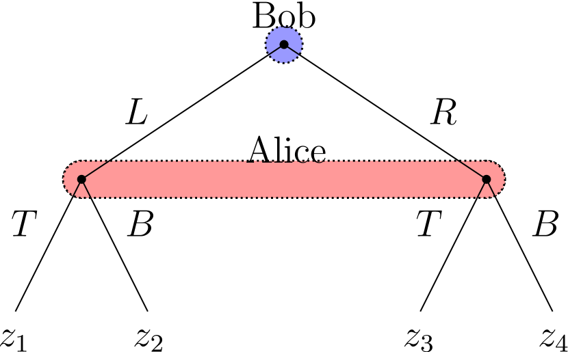
i

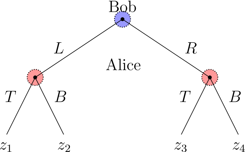
ii

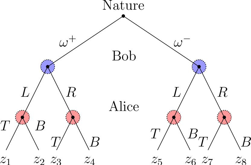
iii

Figure 1: Alice and Bob examples in the tree model

Alice and Bob as unordered agents (trivial information, Figures 1i and 2). In the simplest W-model, we consider two agents $a$ (Alice) and $b$ (Bob) having two possible actions each (top $T$ and bottom $B$ for Alice $a$, left $L$ and right $R$ for Bob $b$), that is,

$${\mathbb{U}}_{a}=\{u_{T},u_{B}\},\quad{\mathbb{U}}_{b}=\{u_{L},u_{R}\}\;.$$ (6a)

We also suppose that Alice and Bob have no information about each other’s actions — see Figure 2 where the two grey disks represent the (here trivial) atoms (that is, the minimal elements for the inclusion order) of the finite $$\sigma \mathcal{I}_{a} \mathcal{I}_{b} \mathcal{I}_{a}=\mathcal{I}_{b}=\{\emptyset,{\mathbb{U}}_{a}\}\otimes\{\emptyset,{\mathbb{U}}_{b}\}$$-fields and — that is, , which can be interpreted as Alice and Bob acting simultaneously. As Nature is absent, the configuration space consists of four elements

$$\mathbb{H}={\mathbb{U}}_{a}\times{\mathbb{U}}_{b}=\{u_{T},u_{B}\}\times\{u_{L},u_{R}\}\;,$$ (6b)

hence the square in Figure 2.

Figure 2: Atoms (grey disks) of the information fields of the agents $a$ and $b$ acting simultaneously (case of Figure 1i)

Alice and Bob as ordered agents (without Nature, Figures 1ii and  3).

As in the previous example, Nature is absent, and there are two agents $a$ (Alice) and $b$ (Bob), having two possible actions each (see (6a)), so that the configuration space consists of four elements (see (6b)). Suppose that Bob’s information field is trivial (Bob knows nothing of Alice’s actions), that is,

$$\mathcal{I}_{b}=\big{\{}\emptyset,\{u_{T},u_{B}\}\}\otimes\{\emptyset,\{u_{L},u_{R}\}\big{\}}$$

(a trivial field represented by its single atom, a grey disk on the right hand side of Figure 3), and that Alice knows what Bob does (Alice can distinguish between $u_{L}$ and $u_{R}$)

$$\mathcal{I}_{a}=\big{\{}\emptyset,\{u_{T},u_{B}\}\}\otimes\{\emptyset,\{u_{L}\},\{u_{R}\},\{u_{L},u_{R}\}\big{\}}$$

(a nontrivial field represented by its two atoms, the two grey vertical ellipses on the left hand side of Figure 3).

In this example, the agents are naturally ordered: Bob plays first, Alice plays second. Had the order been inverted, then there would have been a sort of paradox – Alice would play first, before Bob, and would know Bob’s action that has not been yet taken by him.

Figure 3: Atoms of the information fields of the ordered agents $a$ and $b$, without Nature (case of Figure 1ii)

Alice and Bob as ordered agents (with Nature, Figures 1iii and 4).

In this example, there are two agents $a$ (Alice) and $b$ (Bob) and two states of Nature $\Omega=\{\omega^{+},\omega^{-}\}$ (say, heads or tails). As in the previous examples, agents have two possible actions each (see (6a)). Thus, the configuration space consists of eight elements

$$\mathbb{H}=\{\omega^{+},\omega^{-}\}\times\{u_{T},u_{B}\}\times\{u_{L},u_{R}\}\;,$$

hence the cube in Figure 4. We consider the following information structure:

$$\mathcal{I}_{b} =\overbrace{\big{\{}\emptyset,\{\omega^{+}\},\{\omega^{-}\},\{\omega^{+},\omega^{-}\}\big{\}}}^{\text{Bob knows Nature's move}}\otimes\overbrace{\big{\{}\emptyset,\{u_{T},u_{B}\}\big{\}}}^{\text{Bob does not know what Alice does}}\otimes\{\emptyset,{\mathbb{U}}_{b}\}\;,$$ (7a)

$$\mathcal{I}_{a} =\underbrace{\big{\{}\emptyset,\{\omega^{+}\},\{\omega^{-}\},\{\omega^{+},\omega^{-}\}\big{\}}}_{\text{Alice knows Nature's move}}\otimes\{\emptyset,{\mathbb{U}}_{a}\}\otimes\underbrace{\big{\{}\emptyset,\{u_{L}\},\{u_{R}\},\{u_{L},u_{R}\}\big{\}}}_{\text{Alice knows what Bob does}}\;.$$ (7b)

Again, here agents are naturally ordered: Bob plays first, Alice plays second.

Figure 4: Atoms of the information fields of the ordered agents $a$ and $b$, with Nature (case of Figure 1iii)

Sequential decision-making.

In this example we illustrate the case of continuous action sets. Suppose a player takes her decisions (say, an element of ${\mathbb{R}}^{n}$) at every discrete time step in the set $\llbracket 0,T{-}1\rrbracket$, where $T\geq 1$ is an integer. The situation will be modeled with (possibly) Nature set and field $({\Omega,\mathcal{F}})$, and with $T$ agents in ${\mathbb{A}}=\llbracket 0,T{-}1\rrbracket$, and their corresponding sets, ${\mathbb{U}}_{t}={\mathbb{R}}^{n}$, and fields, $\mathcal{U}_{t}=\mathcal{B}_{{\mathbb{R}}^{n}}$ (the Borel $\sigma$-field of ${\mathbb{R}}^{n}$), for $t\in{\mathbb{A}}$. Then, one builds up the product set $\mathbb{H}=\Omega\times\prod_{t=0}^{T{-}1}{\mathbb{U}}_{t}$ and the product field $\mathcal{H}=\mathcal{F}\otimes\bigotimes_{t=0}^{T{-}1}\mathcal{U}_{t}$. Every agent $t\in\llbracket 0,T{-}1\rrbracket$ is equipped with an information field $\mathcal{I}_{t}\subset\mathcal{H}$. Then, we show how we can express four information patterns: sequentiality, memory of past information, memory of past actions, perfect recall. Following the notation (5b), we set $\mathcal{U}_{\{0,\ldots,t{-}1\}}=\bigotimes_{s=0}^{t-1}\mathcal{U}_{s}\otimes\bigotimes_{s=t}^{T{-}1}\{\emptyset,{\mathbb{U}}_{s}\}$ for $t\in\llbracket 1,T\rrbracket$. The inclusions $\mathcal{I}_{t}\subset\mathcal{H}_{\{0,\ldots,t{-}1\}}=\mathcal{F}\otimes\mathcal{U}_{\{0,\ldots,t{-}1\}}$, for $t\in\llbracket 0,T{-}1\rrbracket$, express that every agent can remember no more than the past actions of the agents before him (sequentiality); memory of past information is represented by the inclusions $\mathcal{I}_{t-1}\subset\mathcal{I}_{t}$, for $t\in\llbracket 1,T{-}1\rrbracket$; memory of past actions is represented by the inclusions $\{\emptyset,\Omega\}\otimes\mathcal{U}_{\{0,\ldots,t{-}1\}}\subset\mathcal{I}_{t}$, for $t\in\llbracket 1,T{-}1\rrbracket$; perfect recall is represented by the inclusions $\mathcal{I}_{t-1}\vee\big{(}{\{\emptyset,\Omega\}\otimes\mathcal{U}_{\{0,\ldots,t{-}1\}}}\big{)}\subset\mathcal{I}_{t}$, for $t\in\llbracket 1,T{-}1\rrbracket$.

To represent $N$ players — where each player $p$ takes a sequence of decisions, one for each period $t\in\llbracket 0,T^{p}{-}1\rrbracket$ — we use $\prod_{p=1}^{N}T^{p}$ agents, labeled by $(p,t)\in\bigcup_{q=1}^{N}\big{(}{\{{q}\}\mathord{\times}\llbracket 0,T^{q}{-}1\rrbracket}\big{)}$. With obvious notations, the inclusions $\mathcal{I}_{({p,t-1})}\subset\mathcal{I}_{({p,t})}$ express memory of one’s own past information, whereas (with obvious notation) the inclusions $\bigvee_{q=1}^{N}\{\emptyset,\Omega\}\otimes\bigotimes_{s=0}^{t-1}\mathcal{U}_{s}^{q}\otimes$ $\bigotimes_{s=t}^{T^{q}-1}\{\emptyset,{\mathbb{U}}_{s}^{q}\}$ $\subset\mathcal{I}_{({p,t})}$ express memory of all players past actions.

Embedding measurability constraints.

We go on with continuous action sets. There are two agents, ${\mathbb{A}}=\{a,b\}$, and Nature is absent, $\Omega=\{0\}$, $\mathcal{F}=\{{\emptyset,\{{0}\}}\}$. The action set of agent $a$ is the unit interval ${\mathbb{U}}_{a}=[0,1]$ equipped with its Borel $\sigma$-algebra $\mathcal{U}_{a}=\mathcal{B}_{[0,1]}$, and agent $a$ does not know what agent $b$ does, represented by $\mathcal{I}_{a}=\{{\emptyset,\mathbb{U}_{a}}\}\otimes\{{\emptyset,\mathbb{U}_{b}}\}$. Agent $b$ has two possible actions — namely $\mathbb{U}_{b}=\{{0,1}\}$, $\mathcal{U}_{b}=2^{\mathbb{U}_{b}}$ — and observes the action of agent $a$, represented by $\mathcal{I}_{b}=\mathcal{B}_{[0,1]}\otimes\{{\emptyset,\mathbb{U}_{b}}\}$. This models ultimatum bargaining (this example is taken from [2, p.157]) where agent $a$ chooses an offer $x$ in the unit interval, which agent $b$ perfectly observes. Then, agent $b$ either accepts the offer $(Y)$ or rejects it $(N)$.

In the model above, consider $A\subset[0,1]$ and a pure “strategy” (mapping) for agent $b$ defined by

$$\lambda_{b}^{A}:x\in[0,1]\mapsto\begin{cases}Y&\text{if}\;x\in A\;,\\ N&\text{if}\;x\not\in A\;.\end{cases}$$

The “strategy” $\lambda_{b}^{A}$ is not a W-strategy when $A\notin\mathcal{B}_{[0,1]}$ (hence the quotes in “strategy”); indeed, condition (3b) is not satisfied since $({\lambda_{b}^{A}})^{-1}\big{(}{\{{Y}\}}\big{)}=A\notin\mathcal{B}_{[0,1]}$. Thus, games in product form can embed measurability constraints to prevent strategies that would lead to no outcomes when combined with expected utilities. But if one is not interested in using probability distributions — as is the case for instance when preferences are not measured by expected utility but by infimal utility (worst-case) — then nothing prevents from choosing the same model, but with $\mathcal{U}_{a}=2^{[0,1]}$ and $\mathcal{I}_{b}=2^{[0,1]}\otimes\left\{\emptyset,\mathbb{U}_{b}\right\}$. Then, in this latter case, the pure “strategy” $\lambda_{b}^{A}$ is a W-strategy.

To stress the point, if one is compelled to use probability distributions over infinite sets, then perfect information — in the sense of $\mathcal{I}_{b}=2^{\mathbb{U}_{a}}\otimes\{{\emptyset,\mathbb{U}_{b}}\}$, where the complete field $2^{\mathbb{U}_{a}}$ represents perfect information — has to be ruled out in favor of $\mathcal{I}_{b}=\mathcal{B}_{[0,1]}\otimes\{{\emptyset,\mathbb{U}_{b}}\}$ — where the Borel field $\mathcal{B}_{[0,1]}$ represents “approximate” perfect information.

2.3 Playability

Regarding Kuhn’s tree formulation, Witsenhausen says that “For any combination of policies one can find the corresponding outcome by following the tree along selected branches, and this is an explicit procedure” [15]. In the Witsenhausen product formulation, there is no such explicit procedure as, for any combination of policies, there may be none, one or many solutions to the (forthcoming) closed-loop equations (10) which express the action of one agent as the output of his strategy, supplied with Nature outcome and with all agents actions. This is why Witsenhausen needs a well-posedness property (that is, the existence and uniqueness of a solution to a set of equations) that he calls solvability in [15], whereas Kuhn does not need it as it is hard-coded in the tree structure. From now on, we will no longer use the terminology of Witsenhausen and we will use playability and playable, where he used solvability and solvable. We indeed think that such vocabulary is more telling to a game theory audience.

2.3.1 Playability

Definition 3.

([15, 16]) A W-model (see Definition 1) is playable if, for every pure W-strategies profile $\lambda=\left(\lambda_{a}\right)_{a\in{\mathbb{A}}}\in\prod_{a\in{\mathbb{A}}}\Lambda_{a}$ and every state of Nature $\omega\in\Omega$, the mapping

$$\lambda\big{(}{\omega,\cdot}\big{)}=\left(\lambda_{a}\big{(}{\omega,\cdot}\big{)}\right)_{a\in{\mathbb{A}}}:\prod_{a\in{\mathbb{A}}}{\mathbb{U}}_{a}\to\prod_{a\in{\mathbb{A}}}{\mathbb{U}}_{a}$$ (8)

has a unique fixed point. In this case, we introduce the solution map

$$S_{\lambda}:\Omega\rightarrow\mathbb{H}$$ (9)

that associates $\omega\in\Omega$ with the unique $h=({\omega,u})=\big{(}{\omega,\left(u_{a}\right)_{a\in{\mathbb{A}}}}\big{)}\in\mathbb{H}$ solution of the closed-loop equations

$$u_{a}=\lambda_{a}\big{(}{\omega,\left(u_{b}\right)_{b\in{\mathbb{A}}}}\big{)}\;,\enspace\forall a\in{\mathbb{A}}\;.$$ (10)

that is,

$$S_{\lambda}(\omega)=h\iff\begin{cases}h_{\emptyset}&=\omega\\ h_{a}&=\lambda_{a}({h})\;,\enspace\forall a\in{\mathbb{A}}\;.\end{cases}$$ (11)

This definition of “playability” is consistent with the term used in [2, p.102]. It corresponds to a well-posedness property, that is, the existence and uniqueness of a solution to the set of equations (10).

Proposition 4.

If a W-model is playable, then

$$\mathcal{I}_{a}\subset\mathcal{H}_{{\mathbb{A}}\setminus\{{a}\}}=\mathcal{F}\otimes\bigotimes\limits_{b\in{\mathbb{A}}\setminus\{{b}\}}\mathcal{U}_{b}\otimes\{\emptyset,{\mathbb{U}}_{a}\}\;,\enspace\forall a\in{\mathbb{A}}\;.$$ (12)

The latter property (12) is referred to as absence of self-information [16, p. 325], that is, that the decision of an agent is not contingent on the decision itself. Technically, it means that, for any agent $a\in{\mathbb{A}}$, a subset in the field $\mathcal{I}_{a}$ is necessarily a cylinder “in the direction ${\mathbb{U}}_{a}$”, that is, that the $a$- coordinate of $\mathcal{I}_{a}$ must always be $\{{\emptyset,{\mathbb{U}}_{a}}\}$ for all agents $a\in{\mathbb{A}}$. In other words, absence of self-information is the property that, for any agent $a\in{\mathbb{A}}$, for any nonempty subset $I_{a}\in\mathcal{I}_{a}$, and for any two configurations $h^{\prime},h^{\prime\prime}\in\mathbb{H}$, we have that

$$h^{\prime}\in I_{a}\,\mbox{ and }\,h^{\prime}_{\emptyset}=h^{\prime\prime}_{\emptyset}\,\mbox{ and }\, \pi_{{\mathbb{A}}\setminus\{{a}\}}h^{\prime}=\pi_{{\mathbb{A}}\setminus\{{a}\}}h^{\prime\prime}\implies h^{\prime\prime}\in I_{a}\;,$$ (13a)

or, equivalently, by (5e)

$$h^{\prime}\in I_{a}\,\mbox{ and }\,h^{\prime}_{\emptyset}=h^{\prime\prime}_{\emptyset}\,\mbox{ and }\, h^{\prime}_{b}=h^{\prime\prime}_{b}\;,\enspace\forall b\in{\mathbb{A}}\setminus\{{a}\}\implies h^{\prime\prime}\in I_{a}\;.$$ (13b)

To avoid paradoxes, absence of self-information is a clear minimal axiomatic requirement that one should ask of a W-model.

As Witsenhausen pointed out that playability implied absence of self-information, but without giving a proof, we provide one below.

Proof.

We consider a playable W-model. To prove (12), we use the characterization (13b). For this purpose, we consider an agent $a\in{\mathbb{A}}$, a nonempty subset $I_{a}\in\mathcal{I}_{a}$, a configuration $h^{\prime}\in I_{a}$, and another configuration $h^{\prime\prime}\in\mathbb{H}$ satisfying $h^{\prime}_{\emptyset}=h^{\prime\prime}_{\emptyset}$, $h^{\prime}_{b}=h^{\prime\prime}_{b}$, $\forall b\in{\mathbb{A}}\setminus\{{a}\}$ and $h^{\prime}\not=h^{\prime\prime}$. We prove that the configuration $h^{\prime\prime}$ necessarily belongs to the subset $I_{a}$.

The proof is by contradiction. Assume that $h^{\prime\prime}\not\in I_{a}$ and define the pure W-strategies profile $\lambda=\left(\lambda_{b}\right)_{b\in{\mathbb{A}}}$ as follows: for any $b\in{\mathbb{A}}\setminus\{{a}\}$, $\lambda_{b}({h})=h^{\prime}_{b}$; $\lambda_{a}({h})=h^{\prime}_{a}$ if $h\in I_{a}$, and $\lambda_{a}({h})=h^{\prime\prime}_{a}$ if $h\not\in I_{a}$. The mapping $\lambda_{a}$ is $\mathcal{I}_{a}$-measurable since $I_{a}\in\mathcal{I}_{a}$; the mapping $\lambda_{b}$ is $\mathcal{I}_{b}$-measurable since $\lambda_{b}$ is constant for $b\in{\mathbb{A}}\setminus\{{a}\}$. As a consequence, $\lambda=\left(\lambda_{b}\right)_{b\in{\mathbb{A}}}$ is a pure W-strategies profile (see Definition 2). Now, we observe that the two (distinct) configurations $h^{\prime}$ and $h^{\prime\prime}$ are fixed point of the W-strategies profile $\lambda$ for the same $\omega=h^{\prime}_{\emptyset}=h^{\prime\prime}_{\emptyset}$. Indeed, first, for the configuration $h^{\prime\prime}$ we have that, for any $b\in{\mathbb{A}}\setminus\{{a}\}$, $\lambda_{b}({h^{\prime\prime}})=h^{\prime}_{b}=h^{\prime\prime}_{b}$ and as $h^{\prime\prime}\not\in I_{a}$ we have that $\lambda_{a}({h^{\prime\prime}})=h^{\prime\prime}_{a}$. Second, for the configuration $h^{\prime}$ we have that, for any $b\in{\mathbb{A}}\setminus\{{a}\}$, $\lambda_{b}({h^{\prime}})=h^{\prime}_{b}$ and, as $h^{\prime}\in I_{a}$, we have that $\lambda_{a}({h^{\prime}})=h^{\prime}_{a}$. Thus, the two configurations $h^{\prime}$ and $h^{\prime\prime}$ are fixed point of the W-strategies profile $\lambda$ for the same $\omega=h^{\prime}_{\emptyset}=h^{\prime\prime}_{\emptyset}$, which contradicts uniqueness (as we also have $h^{\prime}\not=h^{\prime\prime}$) in the Definition 3 of playability.

Therefore, we have proved (by contradiction) that $h^{\prime\prime}\in I_{a}$. As a consequence, we have obtained that $I_{a}\in\mathcal{H}_{{\mathbb{A}}\setminus\{{a}\}}$ and thus $\mathcal{I}_{a}\subset\mathcal{H}_{{\mathbb{A}}\setminus\{{a}\}}$. This ends the proof. ∎

We now present some useful properties of playable W-models. The first one states that the playability property implies a form of partial playability property, by leveraging the fact that any constant strategy is a W-strategy. Let a W-model be playable, let $\lambda=\left(\lambda_{a}\right)_{a\in{\mathbb{A}}}\in\prod\limits_{a\in{\mathbb{A}}}\Lambda_{a}$ be a pure W-strategies profile like in (4a), and let $B\subset{\mathbb{A}}$ be a nonempty subset of agents. From (11), we readily get that

$$\pi_{B}\big{(}{S_{\lambda}({\omega})}\big{)}=\lambda_{B}\big{(}{S_{\lambda}({\omega})}\big{)}\;,\enspace\forall\omega\in\Omega\;,$$ (14)

where the projection $\pi_{B}$ is defined in Equation (5e) and $\lambda_{B}$ is defined in Equation (5f). Now, we examine what happens when we replace some of the W-strategies $\lambda_{a}$ by constant ones. For this purpose, for any subset $B\subset{\mathbb{A}}$ of agents, we introduce the partial solution map $\widehat{S}^{B}_{\lambda_{-B}}$, defined by

$$\widehat{S}^{B}_{\lambda_{-B}}({\omega,u_{B}})=S_{u_{B},\lambda_{-B}}({\omega})\;,\enspace\forall\omega\in\Omega\;,\enspace\forall u_{B}\in{\mathbb{U}}_{B}\;,$$ (15)

where $({u_{B},\lambda_{-B}})$ has to be understood as the pure W-strategies profile made of two subprofiles, like in (5f), namely constant subprofile with values $u_{B}$ and subprofile $\lambda_{-B}=\left(\lambda_{c}\right)_{c\not\in B}\in\prod\limits_{c\not\in B}\Lambda_{c}$.

We obtain the following result, as a straightforward application of (11)–(14)–(15).

Proposition 5.

Let a W-model be playable, as in Definition 3. For any subset $B\subset{\mathbb{A}}$ of agents, the solution map $S_{\lambda}$ in (9) and the partial solution map $\widehat{S}^{B}_{\lambda_{-B}}$ in (15) are related as follows:

$$S_{\lambda}({\omega})=S_{\lambda_{B},\lambda_{-B}}({\omega})=\widehat{S}^{B}_{\lambda_{-B}}\Big{(}{\omega,\pi_{B}\big{(}{S_{\lambda}({\omega})}\big{)}}\Big{)}=\widehat{S}^{B}_{\lambda_{-B}}\Big{(}{\omega,\lambda_{B}\big{(}{S_{\lambda}({\omega})}\big{)}}\Big{)}\;,\enspace\forall\omega\in\Omega\;.$$ (16)

As a consequence, for any two pure W-strategies profiles $\lambda$ and $\lambda^{\prime}$ which are such that $\lambda_{-B}=\lambda^{\prime}_{-B}$, we have that $\widehat{S}^{B}_{\lambda_{-B}}=\widehat{S}^{B}_{\lambda^{\prime}_{-B}}$ and that

$$\bigg{(}{\pi_{B}\big{(}{S_{\lambda}({\omega})}\big{)}=\pi_{B}\big{(}{S_{\lambda^{\prime}}({\omega})}\big{)}\implies S_{\lambda}({\omega})=S_{\lambda^{\prime}}({\omega})}\bigg{)}\;,\enspace\forall\omega\in\Omega\;.$$ (17)

Here is a nice application of property (16), that will be useful in the proof of Kuhn’s equivalence Theorem (Lemma 22).

Proposition 6.

Let a W-model be playable, as in Definition 3. Let $a\in{\mathbb{A}}$ be an agent, and $Z:({\mathbb{H},\mathcal{I}_{a}})\to({\mathbb{Z},\mathcal{Z}})$ be a measurable mapping, where $\mathbb{Z}$ is a set and where the $\sigma$-field $\mathcal{Z}$ contains the singletons. Then, for any pair $\lambda=\left(\lambda_{b}\right)_{b\in{\mathbb{A}}}$ and $\lambda^{\prime}=\left(\lambda^{\prime}_{b}\right)_{b\in{\mathbb{A}}}$ of W-strategy profiles such that $b\neq a\implies\lambda_{b}=\lambda^{\prime}_{b}$, we have that $Z\circ S_{\lambda}=Z\circ S_{\lambda^{\prime}}$.

Proof.

The proof is by contradiction. Let $\lambda=\left(\lambda_{b}\right)_{b\in{\mathbb{A}}}$ and $\lambda^{\prime}=\left(\lambda^{\prime}_{b}\right)_{b\in{\mathbb{A}}}$ be a pair of W-strategy profiles such that $b\neq a\implies\lambda_{b}=\lambda^{\prime}_{b}$, and suppose that there exists $\omega\in\Omega$ such that $Z\big{(}{S_{\lambda}({\omega})}\big{)}\neq Z\big{(}{S_{\lambda^{\prime}}({\omega})}\big{)}$.

Consider $H=Z^{-1}\Big{(}{Z\big{(}{S_{\lambda}({\omega})}\big{)}}\Big{)}\subset\mathbb{H}$. By definition of the subset $H$ and by the very defining property of $\omega\in\Omega$ — that is, $Z\big{(}{S_{\lambda}({\omega})}\big{)}\neq Z\big{(}{S_{\lambda^{\prime}}({\omega})}\big{)}$ — we get that $S_{\lambda}({\omega})\in H$ and $S_{\lambda^{\prime}}({\omega})\not\in H$. Moreover, $H\in\mathcal{I}_{a}$ since $Z:({\mathbb{H},\mathcal{I}_{a}})\to({\mathbb{Z},\mathcal{Z}})$ is a measurable mapping and the $\sigma$-field $\mathcal{Z}$ contains the singletons. We define a new W-strategy $\lambda^{\prime\prime}_{a}$ for agent $a$ as follows:

$$\forall h^{\prime\prime}\in\mathbb{H}\;,\enspace\lambda^{\prime\prime}_{a}({h^{\prime\prime}})=\begin{cases}{\pi_{a}\big{(}{S_{\lambda}({\omega})}\big{)}}&\text{if }h^{\prime\prime}\not\in H\;,\\ {\pi_{a}\big{(}{S_{\lambda^{\prime}}({\omega})}\big{)}}&\text{if }h^{\prime\prime}\in H\;.\end{cases}$$ (18)

Thus defined, the mapping $\lambda^{\prime\prime}_{a}$ indeed is a W-strategy because, as $H\in\mathcal{I}_{a}$, the mapping $\lambda^{\prime\prime}_{a}:(\mathbb{H},\mathcal{I}_{a})\to({\mathbb{U}}_{a},\mathcal{U}_{a})$ is measurable. We define the W-strategies profile $\lambda^{\prime\prime}=\left(\lambda^{\prime\prime}_{b}\right)_{b\in{\mathbb{A}}}$ by completing $\lambda^{\prime\prime}_{a}$ with $\lambda^{\prime\prime}_{b}=\lambda_{b}=\lambda^{\prime}_{b}$ when $b\neq a$.

We prove that playability fails for the W-strategy profile $\lambda^{\prime\prime}$ (hence the contradiction). For this purpose, we consider the following only two possibilities for $S_{\lambda^{\prime\prime}}({\omega})$, depending whether it belongs to $H$ or not.

First, we assume that $S_{\lambda^{\prime\prime}}({\omega})\not\in H$. Then, we have that

$${\pi_{a}\big{(}{S_{\lambda^{\prime\prime}}({\omega})}\big{)}} =\lambda^{\prime\prime}_{a}\big{(}{S_{\lambda^{\prime\prime}}({\omega})}\big{)}$$ (by (14))

$$={\pi_{a}\big{(}{S_{\lambda}({\omega})}\big{)}}\;. S_{\lambda^{\prime\prime}}({\omega})\not\in H$$ (by the first case of (18) as by assumption)

Using Implication (17) with the W-strategies profiles $\lambda^{\prime\prime}$ and $\lambda$ and with the subset $B=\{{a}\}$, we get that $S_{\lambda^{\prime\prime}}({\omega})=S_{\lambda}({\omega})$. Therefore, as $S_{\lambda}({\omega})\in H$, we deduce that $S_{\lambda^{\prime\prime}}({\omega})\in H$, which contradicts the assumption that $S_{\lambda^{\prime\prime}}({\omega})\not\in H$.

Second, we assume that $S_{\lambda^{\prime\prime}}({\omega})\in H$. Then, we have that

$${\pi_{a}\big{(}{S_{\lambda^{\prime\prime}}({\omega})}\big{)}} =\lambda^{\prime\prime}_{a}\big{(}{S_{\lambda^{\prime\prime}}({\omega})}\big{)}$$ (by (14))

$$={\pi_{a}\big{(}{S_{\lambda^{\prime}}({\omega})}\big{)}}\;. S_{\lambda^{\prime\prime}}({\omega})\in H$$ (by the second case of (18) as by assumption)

Using Implication (17) with the W-strategies profiles $\lambda^{\prime\prime}$ and $\lambda^{\prime}$ and with the subset $B=\{{a}\}$, we get that $S_{\lambda^{\prime\prime}}({\omega})=S_{\lambda^{\prime}}({\omega})$. Therefore, as $S_{\lambda^{\prime}}({\omega})\not\in H$, we deduce that $S_{\lambda^{\prime\prime}}({\omega})\not\in H$, which contradicts the assumption that $S_{\lambda^{\prime\prime}}({\omega})\in H$.

We obtain a contradiction and conclude that $Z\big{(}{S_{\lambda}({\omega})}\big{)}=Z\big{(}{S_{\lambda^{\prime}}({\omega})}\big{)}$.

This ends the proof. ∎

Witsenhausen introduced the notion of solvable (here, playable) measurable (SM) property in [15] when the solution map is measurable. We will need a stronger definition.

Definition 7.

Let $B\subset{\mathbb{A}}$ be a nonempty subset of agents. We say that a W-model is playable and partially measurable w.r.t. $B$ if it is playable and, for any subset $B^{\prime}\subset B$, the partial solution map in (15) is a measurable mapping $\widehat{S}^{B^{\prime}}_{\lambda_{-B^{\prime}}}:({\Omega\times{\mathbb{U}}_{B^{\prime}},\mathcal{F}\otimes\mathcal{U}_{B^{\prime}}})\to({\mathbb{H},\mathcal{H}})$, for any pure W-strategies profile $\lambda=\left(\lambda_{a}\right)_{a\in{\mathbb{A}}}\in\prod\limits_{a\in{\mathbb{A}}}\Lambda_{a}$ like in (4a).

Of course, a playable finite W-model is always playable and partially measurable w.r.t. $B$, for any nonempty subset $B\subset{\mathbb{A}}$ of agents.

2.3.2 An example of a playable non causal game: the clapping hand game

Witsenhausen defines the notion of causality and proves in [15] that causality implies playability The reverse, however, is not true. In [15, Theorem 2], Witsenhausen exhibits an example of noncausal W-model that is playable. The construction relies on three agents with binary action sets –hence ${\mathbb{A}}=\{a,b,c\}$, ${\mathbb{U}}_{a}={\mathbb{U}}_{b}={\mathbb{U}}_{c}=\{0,1\}$– and Nature does not play any role – so that $\mathbb{H}=\{0,1\}^{3}$. The example (see Figure 5) relies on a choice of information fields so that (i) no information field is trivial — which means that there is no first agent — (ii) the W-model is playable though. The triplet of information fields

$$\mathcal{I}_{a} =\Big{\{}{\emptyset,\{{0,1}\}^{3},\big{\{}{({0,1,0}),({1,1,0})}\big{\}},\big{\{}{({0,0,0}),({1,0,0}),({0,0,1}),({1,0,1}),({0,1,1}),({1,1,1})}\big{\}}}\Big{\}}$$

$$\mathcal{I}_{b} =\Big{\{}{\emptyset,\{{0,1}\}^{3},\big{\{}{({0,1,1}),({0,0,1})}\big{\}},\big{\{}{({0,0,0}),({0,1,0}),({1,0,0}),({1,1,0}),({1,0,1}),({1,1,1})}\big{\}}}\Big{\}}$$

$$\mathcal{I}_{c} =\Big{\{}{\emptyset,\{{0,1}\}^{3},\big{\{}{({1,0,0}),({1,0,1})}\big{\}},\big{\{}{({0,0,0}),({0,0,1}),({0,1,0}),({0,1,1}),({1,1,0}),({1,1,1})}\big{\}}}\Big{\}}$$

— that is, $\mathcal{I}_{a}=\sigma(\pi_{b}(1-\pi_{c}))\;,\enspace\mathcal{I}_{b}=\sigma(\pi_{c}(1-\pi_{a}))\;,\enspace\mathcal{I}_{c}=\sigma(\pi_{a}(1-\pi_{b}))$ (where $\sigma$ denotes the $\sigma$-field generated by a measurable mapping, here built up from the projections $\pi_{a}$, $\pi_{b}$, $\pi_{c}$ defined in Equation (5e)) — clearly satisfies (i). Let us show that playability holds. First we observe that the W-strategies can be written as

$$\lambda_{a}({u_{a},u_{b},u_{c}})=\widetilde{\lambda}_{a}\big{(}{u_{b}(1-u_{c})}\big{)},\;\lambda_{b}({u_{a},u_{b},u_{c}})=\widetilde{\lambda}_{b}\big{(}{u_{c}(1-u_{a})}\big{)},\;\lambda_{c}({u_{a},u_{b},u_{c}})=\widetilde{\lambda}_{c}\big{(}{u_{a}(1-u_{b})}\big{)},$$

where $\widetilde{\lambda}:\{0,1\}\to\{0,1\}$, hence $({\widetilde{\lambda}_{a},\widetilde{\lambda}_{b},\widetilde{\lambda}_{c}})\in\{\textrm{Id},1-\textrm{Id}\}^{3}$ (Id denotes the identity mapping). From there, we check that playability holds true, with the (constant) solution map given by

$$S_{({\textrm{Id},\textrm{Id},\textrm{Id}})}=({0,0,0}),\;S_{({1-\textrm{Id},\textrm{Id},\textrm{Id}})}=({1,0,1}),\;S_{({1-\textrm{Id},1-\textrm{Id},\textrm{Id}})}=({0,1,0}),\;S_{({1-\textrm{Id},1-\textrm{Id},1-\textrm{Id}})}=({1,1,1}).$$

Hence the W-model is noncausal (because there is no first agent) but playable.

Figure 5: Noncausal playable W-model: information partitions of the three agents

This model can be illustrated by the following “clapping hands” story. Alice, Bob and Carol are sitting around a circular table, with their eyes closed. Each of them has to decide either to extend her/his left hand to the left or to extend her/his right hand to the right. When two hands touch, the remaining player is informed (say, a clap is directly conveyed to her/his ears); when two hands do not touch, the remaining player is not informed. For each triplet of strategies — one for each of Alice, Bob and Carol — there is a unique outcome of extended hands: the game is playable. However, the game cannot start.

Hence a game can be well-posed (playable), but yet miss the crucial feature of being implementable in practice. Fortunately, Witsenhausen provides in [15] sufficient conditions (causality) to rule out such (pathological) cases.

Witsenhausen’s intrinsic model deals with agents, information and strategies, but not with players and preferences. We now turn to extending the Witsenhausen’s intrinsic model to games.

3 Games in product form

We are now ready to embed Witsenhausen’s intrinsic model into game theory. In §3.1, we introduce a formal definition of a game in product form (W-game). In §3.2, we define mixed and behavioral strategies in the spirit of Aumann [3].

3.1 Definition of a game in product form (W-game)

We introduce a formal definition of a game in product form (W-game).

Definition 8.

A W-game $\Big{(}{\big{(}{\left({\mathbb{A}}^{p}\right)_{p\in P},({\Omega,\mathcal{F}}),\left({\mathbb{U}}_{a},\mathcal{U}_{a},\mathcal{I}_{a}\right)_{a\in{\mathbb{A}}}}\big{)},(\precsim^{p})_{p\in P}}\Big{)}$, or a game in product form, is made of

• a set ${\mathbb{A}}$ of agents with a partition $\left({\mathbb{A}}^{p}\right)_{p\in P}$, where $P$ is the set of players; each subset ${\mathbb{A}}^{p}$ is interpreted as the subset of executive agents of the player $p\in P$;

• a W-model (called underlying W-model) $\big{(}{{\mathbb{A}},({\Omega,\mathcal{F}}),\left({\mathbb{U}}_{a},\mathcal{U}_{a},\mathcal{I}_{a}\right)_{a\in{\mathbb{A}}}}\big{)}$, as in Definition 1;

• for each player $p\in P$, a preference relation $\precsim^{p}$ on $\Delta(\mathbb{H},\mathcal{H})$, the set of probability distributions on $\mathbb{H}$.

Let $p\in P$ be a player. A W-game is said to be playable (resp. playable and partially measurable w.r.t. $p$), if the underlying W-model is playable as in Definition 3 (resp. playable and partially measurable w.r.t. ${\mathbb{A}}^{p}$ as in Definition 7).

A finite W-game is a W-game whose underlying W-model is finite. In a W-game, the family $\left({\mathbb{A}}^{p}\right)_{p\in P}$ consists of pairwise disjoint nonempty sets whose union is ${\mathbb{A}}=\bigcup_{p\in P}{\mathbb{A}}^{p}$. When we focus on a specific player $p\in P$, we denote ${\mathbb{A}}^{-p}=\bigcup_{q\in P\setminus\{{p}\}}{\mathbb{A}}^{q}$. In what follows, agents appear as lower indices and (most of the time) players as upper indices.

With the above definition, we cover (like in [5]) the most traditional preference relation $\precsim^{p}$, which is the numerical expected utility preference. In this latter, each player $p\in P$ is endowed, on the one hand, with a criterion (payoff, objective function), that is, a measurable function $J^{p}:(\mathbb{H},\mathcal{H})\rightarrow[-\infty,+\infty[$ (we include $-\infty$ in the codomain of the criterion as a way to handle constraints) which is bounded above, and, on the other hand, with a belief, that is, a probability distribution $\nu^{p}:\mathcal{F}\rightarrow[0,1]$ over the states of Nature $(\Omega,\mathcal{F})$. Then, given two measurable mappings $S_{i}:({\Omega,\mathcal{F}})\to\Delta({{\mathbb{U}}_{\mathbb{A}},\mathcal{U}_{\mathbb{A}}})$, $i=1,2$, one says that $S_{1}\precsim^{p}S_{2}$ if $\int_{\Omega}\nu^{p}({d\omega})\int_{{\mathbb{U}}_{\mathbb{A}}}J^{p}({\omega,u})S_{1}({\omega,\,\mathrm{d}u})\leq\int_{\Omega}\nu^{p}({d\omega})\int_{{\mathbb{U}}_{\mathbb{A}}}J^{p}({\omega,u})S_{1}({\omega,\,\mathrm{d}u})$ where both integrals are well defined in $[-\infty,+\infty[$ because the function $J^{p}$ is supposed to be bounded above.

The preference relation $\precsim^{p}$ need not be over probability distributions. This is the case in the infimal utility (worst-case) setting, where each player $p\in P$ is only endowed with a criterion $J^{p}:(\mathbb{H},\mathcal{H})\rightarrow[-\infty,+\infty]$, not necessarily a measurable function. Then, given two mappings $S_{i}:\Omega\to\mathbb{H}$, $i=1,2$, not necessarily measurable, one says that $S_{1}\precsim^{p}S_{2}$ if $\inf_{\omega\in\Omega}J^{p}\big{(}{S_{1}(\omega)}\big{)}\leq\inf_{\omega\in\Omega}J^{p}\big{(}{S_{2}(\omega)}\big{)}$.

Note also that Definition 8 can encompass Bayesian games, by specifying a product structure $\Omega=\Omega^{0}\times\prod_{p\in P}\Omega^{p}$ — where one factor $\Omega^{0}$ may represent chance, and the others $\Omega^{p}$ may represent types of players — and a probability on $\Omega$.

3.2 Mixed and behavioral strategies

We define mixed and behavioral strategies in the spirit of Aumann in [3], using the vocable of A-pure, A-mixed and A-behavioral strategies (with A- as a reference to Aumann).

For this purpose, for any agent $a\in{\mathbb{A}}$, we denote by $\big{(}{\mathbb{W}_{a},\mathcal{W}_{a}}\big{)}$ a copy of the Borel space $\big{(}{[0,1],\mathcal{B}_{[0,1]}}\big{)}$, by $\ell_{a}$ a copy of the Lebesgue measure on $\big{(}{\mathbb{W}_{a},\mathcal{W}_{a}}\big{)}=\big{(}{[0,1],\mathcal{B}_{[0,1]}}\big{)}$, and we also set

$$\mathbb{W}^{p}=\prod_{a\in{\mathbb{A}}^{p}}\mathbb{W}_{a}\;,\enspace\mathcal{W}^{p}=\bigotimes_{a\in{\mathbb{A}}^{p}}\mathcal{W}_{a}\;,\enspace\ell^{p}=\bigotimes_{a\in{\mathbb{A}}^{p}}\ell_{a}\;,\enspace\forall p\in P$$ (19a)

and

$$\mathbb{W}=\prod_{p\in P}\mathbb{W}^{p}\;,\enspace\mathcal{W}=\bigotimes_{p\in P}\mathcal{W}^{p}\;,\enspace\ell=\bigotimes_{p\in P}\ell^{p}\;.$$ (19b)

The existence of a product probability space $(\mathbb{W},\mathcal{W},\ell)$, that is, the existence of a product space $\mathbb{W}$ equipped with a product $\sigma$-algebra $\mathcal{W}$ and a probability measure $\ell$ with $\ell_{a}$ as marginal probability for each agent $a\in{\mathbb{A}}$ is developed in [1, §15.6] and is, in the case we consider, a consequence of the Kolmogorov extension theorem.

Definition 9.

For the player $p\in P$, an A-mixed strategy is a family $m^{p}=\left(m^{p}_{a}\right)_{a\in{\mathbb{A}}^{p}}$ of measurable mappings

$$m^{p}_{a}:\big{(}{\prod_{b\in{\mathbb{A}}^{p}}\mathbb{W}_{b}\times\mathbb{H},\bigotimes_{b\in{\mathbb{A}}^{p}}\mathcal{W}_{b}\otimes\mathcal{I}_{a}}\big{)}\to({{\mathbb{U}}_{a},\mathcal{U}_{a}})\;,\enspace\forall a\in{\mathbb{A}}^{p}\;,$$ (20a)

an A-behavioral strategy is an A-mixed strategy $m^{p}=\left(m^{p}_{a}\right)_{a\in{\mathbb{A}}^{p}}$ with the property that

$$({m^{p}_{a}})^{-1}({\mathcal{U}_{a}})\subset\big{(}{\mathcal{W}_{a}\otimes\bigotimes_{b\in{\mathbb{A}}^{p}\setminus\{{a}\}}\{{\emptyset,\mathbb{W}_{b}}\}}\big{)}\otimes\mathcal{I}_{a}\;,\enspace\forall a\in{\mathbb{A}}^{p}\;,$$ (20b)

and an A-pure strategy is an A-mixed strategy $m^{p}=\left(m^{p}_{a}\right)_{a\in{\mathbb{A}}^{p}}$ with the property that

$$({m^{p}_{a}})^{-1}({\mathcal{U}_{a}})\subset\bigotimes_{b\in{\mathbb{A}}^{p}}\{{\emptyset,\mathbb{W}_{b}}\}\otimes\mathcal{I}_{a}\;,\enspace\forall a\in{\mathbb{A}}^{p}\;.$$ (20c)

An A-mixed strategy profile is a family $m=\left(m^{p}\right)_{p\in P}$ of A-mixed strategies.

By definition, A-behavioral strategies form a subset of A-mixed strategies. Equation (20b) means that, for any agent $a$ and any fixed configuration $h\in\mathbb{H}$, $m^{p}_{a}({w^{p},h})$ only depends on the randomizing component ${w}_{a}$. Thus, under the product probability distribution $\ell^{p}=\bigotimes_{a\in{\mathbb{A}}^{p}}\ell_{a}$ in (19b), the random variables $\left(m^{p}_{a}({\cdot,h})\right)_{a\in{\mathbb{A}}^{p}}$ are independent. In other words, an A-behavioral strategy is an A-mixed strategy in which the randomization is made independently, agent by agent, for each fixed configuration $h\in\mathbb{H}$. An A-pure strategy is an A-mixed strategy in which there is no randomization, hence can be identified with a pure W-strategy as in Definition 2.

The connection between A-mixed strategies profiles and pure W-strategies profiles, as in (4a), is as follows: if $m^{p}=\left(m^{p}_{a}\right)_{a\in{\mathbb{A}}^{p}}$ is an A-mixed strategy (20a), then every mapping

$$m^{p}_{a}({w^{p},\cdot}):({\mathbb{H},\mathcal{I}_{a}})\to({{\mathbb{U}}_{a},\mathcal{U}_{a}})\;,\enspace h\mapsto m^{p}_{a}({w^{p},h})\;,\enspace\forall w^{p}=\left(w_{b}\right)_{b\in{\mathbb{A}}^{p}}\in\mathbb{W}^{p}=\prod_{b\in{\mathbb{A}}^{p}}\mathbb{W}_{b}$$

belongs to $\Lambda_{a}$ (see (3b)), for $a\in{\mathbb{A}}^{p}$, and thus $\left(m^{p}_{a}({w^{p},\cdot})\right)_{a\in{\mathbb{A}}^{p}}\in\Lambda^{p}=\prod_{a\in{\mathbb{A}}^{p}}\Lambda_{a}$. In the same way, an A-mixed strategy profile $m=\left(m^{p}\right)_{p\in P}$ induces, for any $w\in\mathbb{W}$, a mapping $m({w,\cdot})\in\Lambda=\prod_{a\in{\mathbb{A}}}\Lambda_{a}$ in (4b).

Consider a playable W-model (see Definition 3), and a profile $m=\left(m^{p}\right)_{p\in P}$ of A-mixed strategies. For any $w\in\mathbb{W}$, $m({w,\cdot})$ is a pure strategy and $S_{m({w,\cdot})}({\omega})$ is well defined by playability We use the following compact notation for the solution map as in (9):

$$T^{\omega}_{m}({w}) =S_{m({w,\cdot})}({\omega})\;,\enspace\forall\omega\in\Omega\;,\enspace\forall w\in\mathbb{W}\;.$$ (21)

As we introduce A-mixed strategies, we need to adapt the definition of solvable measurable (SM) property in [15]. To stress the difference, the notion below is for W-games (to distinguish it from a possible definition for W-models inspired by the SM property in [15]).

Definition 10.

We say that a W-game is playable and measurable if, for any profile $m=\left(m^{p}\right)_{p\in P}$ of A-mixed strategies, the following mapping is measurable

$$T_{m}:({\mathbb{W}\times\Omega,\mathcal{W}\otimes\mathcal{F}})\to({\mathbb{H},\mathcal{H}})\;,\enspace({w,\omega})\mapsto T^{\omega}_{m}({w})\;,$$ (22)

where $T^{\omega}_{m}({w})$ is defined in Equation (21). In that case, for any probability $\nu$ on $({\Omega,\mathcal{F}})$, we denote by

$${\mathbb{Q}}^{\nu}_{m}={\mathbb{Q}}^{\nu}_{({m^{p}})_{p\in P}}=\Big{(}{\big{(}{\bigotimes_{p\in P}\ell^{p}}\big{)}\otimes\nu}\Big{)}\circ({T_{({m^{p}})_{p\in P}}})^{-1}=({\ell\otimes\nu})\circ({T_{m}})^{-1}$$ (23)

the pushforward probability, on the space $({\mathbb{H},\mathcal{H}})$, of the product probability distribution $\ell\otimes\nu=\big{(}{\bigotimes_{p\in P}\ell^{p}}\big{)}\otimes\nu$ on $\mathbb{W}\times\Omega=\big{(}{\prod_{p\in P}\mathbb{W}^{p}}\big{)}\times\Omega$ by the mapping $T_{m}$ in (21).

Of course, a playable finite W-game is always playable and measurable.

4 Kuhn’s equivalence theorem

In this section, we provide, for games in product form, a statement and a proof of the celebrated Kuhn’s equivalence theorem: when a player satisfies perfect recall, for any mixed W-strategy, there is an equivalent behavioral strategy (and the converse). We start by adapting, in §4.1, the definition of perfect recall to games in product forms and by illustrating the soundness of this new definition with Proposition 15. Then, in §4.2, we outline the main results.

4.1 Perfect recall in W-games

For any agent $a\in{\mathbb{A}}$, we define the choice field $\mathcal{C}_{a}\subset\mathcal{H}$ as the least upper bound of the action field $\mathcal{U}_{a}$ and of the information field $\mathcal{I}_{a}$, namely

$$\mathcal{C}_{a}=\mathcal{U}_{a}\bigvee\mathcal{I}_{a}\;,\enspace\forall a\in{\mathbb{A}}\;.$$ (24)

Thus defined, the choice field of agent $a$ contains both what the agent did ($\mathcal{U}_{a}$ identified with $\mathcal{U}_{\{{a}\}}$) and what he knew ($\mathcal{I}_{a}$) when taking a decision. As formulated, our definition is close to the notion of choice in [2, Definition 4.1].

We consider a focus player $p\in P$ and we suppose that the set ${\mathbb{A}}^{p}$ of her executive agents is finite with cardinality $\left|{\mathbb{A}}^{p}\right|$. For any $k\in\llbracket 1,\left|{\mathbb{A}}^{p}\right|\rrbracket$, let $\Sigma^{p}_{k}$ denote the set of $k$-orderings of player $p$, that is, injective mappings from $\llbracket 1,k\rrbracket$ to ${\mathbb{A}}^{p}$:

$$\Sigma^{p}_{k}=\big{\{}{\kappa:\llbracket 1,k\rrbracket\to{\mathbb{A}}^{p}\,\big{|}\,\kappa\,\mbox{ is an injection}\,}\big{\}}\;.$$ (25a)

We define the set of orderings of player $$p p$$, shortly set of -orderings, by

$$\Sigma^{p}=\bigcup_{k=1}^{\left|{\mathbb{A}}^{p}\right|}\Sigma^{p}_{k}\;.$$ (25b)

The set $\Sigma^{p}_{\left|{\mathbb{A}}^{p}\right|}$ is the set of total orderings of player $p$, shortly total $p$-orderings, of agents in ${\mathbb{A}}^{p}$, that is, bijective mappings from $\llbracket 1,\left|{\mathbb{A}}^{p}\right|\rrbracket$ to ${\mathbb{A}}^{p}$ (in contrast with $p$-partial orderings in $\Sigma^{p}_{k}$ for $k<\left|{\mathbb{A}}^{p}\right|$). For any $k\in\llbracket 1,\left|{\mathbb{A}}^{p}\right|\rrbracket$, any $p$-ordering $\kappa\in\Sigma^{p}_{k}$, and any $i\in\llbracket 1,k\rrbracket$, $\kappa_{|\llbracket 1,i\rrbracket}\in\Sigma^{p}_{i}$ is the restriction of the $p$-ordering $\kappa$ to the first $i$ integers. For any $k\in\llbracket 1,\left|{\mathbb{A}}^{p}\right|\rrbracket$, there is a natural mapping

$$\psi_{k}:\Sigma^{p}_{\left|{\mathbb{A}}^{p}\right|}\to\Sigma^{p}_{k}\;,\enspace\rho\mapsto\rho_{|\llbracket 1,k\rrbracket}\;,$$ (26)

which is the restriction of any (total) $p$-ordering of ${\mathbb{A}}^{p}$ to $\llbracket 1,k\rrbracket$. For any $k\in\llbracket 1,\left|{\mathbb{A}}^{p}\right|\rrbracket$, we define the range $\|\kappa\|$ of the $p$-ordering $\kappa\in\Sigma^{p}_{k}$ as the subset of agents

$$\|\kappa\| =\big{\{}{\kappa(1),\ldots,\kappa(k)}\big{\}}\subset{\mathbb{A}}^{p}\;,\enspace\forall\kappa\in\Sigma^{p}_{k}\;,$$ (27a)

the cardinality $$\left|\kappa\right| p \kappa\in\Sigma^{p}_{k}$$ of the -ordering  as the integer

$$\left|\kappa\right| =k\in\llbracket 1,\left|{\mathbb{A}}^{p}\right|\rrbracket\;,\enspace\forall\kappa\in\Sigma^{p}_{k}\;,$$ (27b)

the last element $${\kappa}_{\star} p \kappa\in\Sigma^{p}_{k}$$ of the -ordering  as the agent

$${\kappa}_{\star} =\kappa(k)\in{\mathbb{A}}^{p}\;,\enspace\forall\kappa\in\Sigma^{p}_{k}\;,$$ (27c)

the first elements $${\kappa}_{-} p \kappa\in\Sigma^{p}_{k} k{-}1$$ as the restriction of the -ordering  to the first elements

$${\kappa}_{-} =\kappa_{|\llbracket 1,k{-}1\rrbracket}\in\Sigma^{p}_{k-1}\;,\enspace\forall\kappa\in\Sigma^{p}_{k}\;,$$ (27d)

with the convention that ${\kappa}_{-}=\emptyset\in\Sigma^{p}_{0}=\{\emptyset\}$ when $\kappa\in\Sigma^{p}_{1}$. With obvious notation, any $p$-ordering $\kappa\in\Sigma^{p}$ can be written as $\kappa=({{\kappa}_{-},{\kappa}_{\star}})$, with the convention that $\kappa=({{\kappa}_{\star}})$ when $\kappa\in\Sigma_{1}^{p}$.

The following notion of configuration-ordering is adapted from [15, Property C, p. 153].

Definition 11.

We consider a focus player $p\in P$ and we suppose that the set ${\mathbb{A}}^{p}$ of her executive agents is finite. A $p$-configuration-ordering is a mapping $\varphi:\mathbb{H}\to\Sigma^{p}_{\left|{\mathbb{A}}^{p}\right|}$ from configurations to total $p$-orderings. With any $p$-configuration-ordering $\varphi$, and any $p$-ordering $\kappa\in\Sigma^{p}$, we associate the subset $\mathbb{H}_{\kappa}^{\varphi}\subset\mathbb{H}$ of configurations defined by

$$\mathbb{H}_{\kappa}^{\varphi}=\big{\{}{h\in\mathbb{H}\,\big{|}\,\psi_{\left|\kappa\right|}\big{(}{\varphi(h)}\big{)}=\kappa}\big{\}}\;,\enspace\forall\kappa\in\Sigma^{p}\;.$$ (28)

By convention, we put $\mathbb{H}_{\emptyset}^{\varphi}=\mathbb{H}$.

Thus, the set $\mathbb{H}_{\kappa}^{\varphi}$ is made of configurations along which agents are ordered by $\kappa$

The following definition of perfect recall is new.

Definition 12.

We say that a player $p\in P$ in a W-model satisfies perfect recall if the set ${\mathbb{A}}^{p}$ of her executive agents is finite and if there exists a $p$-configuration-ordering $\varphi:\mathbb{H}\to\Sigma^{p}_{\left|{\mathbb{A}}^{p}\right|}$ such that

$$\mathbb{H}_{\kappa}^{\varphi}\cap H\in\mathcal{I}_{{\kappa}_{\star}}\;,\enspace\forall H\in\mathcal{C}_{\|{\kappa}_{-}\|}\;,\enspace\forall\kappa\in\Sigma^{p}\;,$$ (29a)

where the subset $$\mathbb{H}_{\kappa}^{\varphi}\subset\mathbb{H} {\kappa}_{\star} p {\kappa}_{-} \Sigma^{p}$$ of configurations has been defined in (28), the last agent  in (27c), the -ordering  in (27d), the set  in (25b), and where

$$\mathcal{C}_{\|{\kappa}_{-}\|}=\bigvee\limits_{a\in\|{\kappa}_{-}\|}\mathcal{C}_{a}=\bigvee\limits_{a\in\|{\kappa}_{-}\|}\mathcal{U}_{a}\vee\mathcal{I}_{a}\subset\mathcal{H}\;.$$ (29b)

Under perfect recall, we will use the property that $\mathbb{H}_{\kappa}^{\varphi}\in\mathcal{I}_{{\kappa}_{\star}}$, by (29b) with $H=\mathbb{H}$.

We interpret the above definition as follows. A player satisfies perfect recall if each of her agents, when called upon to move last at a given ordering, remembers everything that his predecessors (according to the ordering), who belong to the same player, knew ($\mathcal{I}_{a}$) and did ($\mathcal{U}_{a}$ identified with $\mathcal{U}_{\{{a}\}}$).

This definition is very close in spirit to the definitions proposed in [11, Definition 203.3], [3] and [13], that rely on “recording” or “recall” functions (whereas (29b) involves $\sigma$-fields). To illustrate the definition, let us revisit Alice and Bob examples in §2.2. If we consider that Alice and Bob are agents of the same player, then perfect recall is satisfied in the second case (one acting after another as in Figures 1ii and 3) and third case (acting after the Nature’s move as in Figures 1iii and 4), but not in the first case (acting simultaneously as in Figures 1i and 2) because neither Alice nor Bob knows which action the other made.

We are going to show, in Proposition 15 to come, that perfect recall implies the existence of a temporal ordering of the agents of the focus player. For this purpose, we introduce the following definition of partial causality, inspired by the property of causality in [15, Property C, p. 153] (and slightly generalized in [16, p. 324]). For any player $p\in P$, we set the fields

$$\mathcal{H}_{B}^{p}=\mathcal{F}\otimes\bigotimes\limits_{b\in B}\mathcal{U}_{b}\otimes\bigotimes\limits_{a\in{\mathbb{A}}^{p}\setminus B}\{\emptyset,{\mathbb{U}}_{a}\}\otimes\bigotimes\limits_{c\not\in{\mathbb{A}}^{p}}\mathcal{U}_{c}\subset\mathcal{H}\;,\enspace\forall B\subset{\mathbb{A}}^{p}\;,$$ (30)

which represents the knowledge of the actions of all agents, except those in ${\mathbb{A}}^{p}\setminus B$.

Definition 13.

We say that a player $p\in P$ in a W-model satisfies partial causality if the set ${\mathbb{A}}^{p}$ of her executive agents is finite and if there exists a $p$-configuration-ordering $\varphi:\mathbb{H}\to\Sigma^{p}_{\left|{\mathbb{A}}^{p}\right|}$ such that

$$\mathbb{H}_{\kappa}^{\varphi}\cap H\in\mathcal{H}_{\|{\kappa}_{-}\|}^{p}\;,\enspace\forall H\in\mathcal{I}_{{\kappa}_{\star}}\;,\enspace\forall\kappa\in\Sigma^{p}\;,$$ (31)

where the subset $\mathbb{H}_{\kappa}^{\varphi}\subset\mathbb{H}$ of configurations has been defined in (28), the last agent ${\kappa}_{\star}$ in (27c), the $p$-ordering ${\kappa}_{-}$ in (27d), the set $\Sigma^{p}$ in (25b), and $\mathcal{H}_{\|{\kappa}_{-}\|}^{p}$ in (30). When $\kappa\in\Sigma^{p}_{1}$, $\mathcal{H}_{\|{\kappa}_{-}\|}^{p}=\mathcal{H}_{\emptyset}^{p}=\mathcal{F}\otimes\bigotimes\limits_{a\in{\mathbb{A}}^{p}}\{\emptyset,{\mathbb{U}}_{a}\}\otimes\bigotimes\limits_{c\not\in{\mathbb{A}}^{p}}\mathcal{U}_{c}=\mathcal{F}\otimes\mathcal{U}_{{\mathbb{A}}^{-p}}$.

Intuitively, the information of the last agent (in a partial ordering) cannot depend on the actions of agents with greater order.

The following Lemma 14 will be instrumental in the coming proofs.

Lemma 14.

Suppose that player $p\in P$ satisfies partial causality with $p$-configuration-ordering $\varphi:\mathbb{H}\to\Sigma^{p}$. Let $\kappa\in\Sigma^{p}$ be a $p$-ordering. Then, for any integer $j\in\llbracket 1,\left|\kappa\right|\rrbracket$ and for any $\mathcal{I}_{\kappa({j})}$-measurable mapping $Z:({\mathbb{H},\mathcal{H}})\to({\mathbb{Z},\mathcal{Z}})$ — where $\mathbb{Z}$ is a set and where the $\sigma$-field $\mathcal{Z}$ contains the singletons — we have the property that

$$h^{\prime}\in\mathbb{H}\;,\enspace h\in\mathbb{H}_{\kappa({1}),\ldots,\kappa({j-1})}^{\varphi}\;,\enspace({h_{\emptyset},h_{{\mathbb{A}}^{-p}},h_{\kappa({1})},\ldots,h_{\kappa({j{-}1})}})=({h^{\prime}_{\emptyset},h^{\prime}_{{\mathbb{A}}^{-p}},h^{\prime}_{\kappa({1})},\ldots,h^{\prime}_{\kappa({j{-}1})}})$$

$$\implies h^{\prime}\in\mathbb{H}_{\kappa({1}),\ldots,\kappa({j-1})}^{\varphi}\,\mbox{ and }\,Z({h^{\prime}})=Z({h})\;,$$ (32a)

which we shortly denote by

$$Z({h})=Z({h_{\emptyset},h_{{\mathbb{A}}^{-p}},h_{\kappa({1})},\ldots,h_{\kappa({j{-}1})}})\;,\enspace\forall h\in\mathbb{H}_{\kappa({1}),\ldots,\kappa({j-1})}^{\varphi}\;,$$ (32b)

where the right-hand side means the common value $Z({h_{\emptyset},h_{{\mathbb{A}}^{-p}},h_{\kappa({1})},\ldots,h_{\kappa({j{-}1})},h^{\prime}_{{\mathbb{A}}^{p}\setminus\{{\kappa({1}),\ldots,\kappa({j{-}1})}\}}})$ for any $h^{\prime}_{{\mathbb{A}}^{p}\setminus\{{\kappa({1}),\ldots,\kappa({j{-}1})}\}}$.

Proof.

Suppose that player $p$ satisfies partial causality with $p$-configuration-ordering $\varphi:\mathbb{H}\to\Sigma^{p}$. Let $\kappa\in\Sigma^{p}$, $j\in\llbracket 1,\left|\kappa\right|\rrbracket$ and $Z:({\mathbb{H},\mathcal{H}})\to({\mathbb{Z},\mathcal{Z}})$ be a $\mathcal{I}_{\kappa({j})}$-measurable mapping. For any configuration $h\in\mathbb{H}_{\kappa({1}),\ldots,\kappa({j-1})}^{\varphi}$, the set $Z^{-1}\big{(}{Z({h})}\big{)}$ contains $h$ and belongs to $\mathcal{I}_{\kappa({j})}$, by the measurability assumption on the mapping $Z$ and the assumption that the $\sigma$-field $\mathcal{Z}$ contains the singletons. By partial causality (31), we get that $\mathbb{H}_{\kappa({1}),\ldots,\kappa({j-1})}^{\varphi}\cap Z^{-1}\big{(}{Z({h})}\big{)}\in\mathcal{H}_{\kappa({1}),\ldots,\kappa({j-1})}^{p}$. By definition (30) of this latter field, the set $\mathbb{H}_{\kappa({1}),\ldots,\kappa({j-1})}^{\varphi}\cap Z^{-1}\big{(}{Z({h})}\big{)}$ is a cylinder such that, if $h^{\prime}\in\mathbb{H}$ and $({h_{\emptyset},h_{{\mathbb{A}}^{-p}},h_{\kappa({1})},\ldots,h_{\kappa({j{-}1})}})=({h^{\prime}_{\emptyset},h^{\prime}_{{\mathbb{A}}^{-p}},h^{\prime}_{\kappa({1})},\ldots,h^{\prime}_{\kappa({j{-}1})}})$, then $h^{\prime}\in\mathbb{H}_{\kappa({1}),\ldots,\kappa({j-1})}^{\varphi}\cap Z^{-1}\big{(}{Z({h})}\big{)}$. Therefore, we have gotten (32a). ∎

Now, we show that perfect recall implies the existence of a temporal ordering of the agents of the focus player.

Proposition 15.

In a playable W-model, if a player satisfies perfect recall with some configuration-ordering, then she satisfies partial causality with the same configuration-ordering.

Proof.

The proof is by contradiction. We will show that, if a player satisfies perfect recall with some configuration-ordering and that she does not satisfy partial causality with the same configuration-ordering, then necessarily there would exist an agent $b\in{\mathbb{A}}^{p}$ such that $\mathcal{I}_{b}\not\subset\mathcal{H}_{{\mathbb{A}}\setminus\{{b}\}}$ (see Equation (5c)). Now, as proved in Proposition 4, in a playable W-model, all agents satisfy absence of self-information, namely any agent $a\in{\mathbb{A}}$ is such that $\mathcal{I}_{a}\subset\mathcal{H}_{{\mathbb{A}}\setminus\{{a}\}}$. Therefore, we will obtain a contradiction as it is assumed that the W-model is playable.

We now give the details. Using Definition 29 of perfect recall, there exists a configuration-ordering $\varphi:\mathbb{H}\to\Sigma^{p}$ such that (29b) holds true. We suppose that player $p$ is not partially causal for this very configuration-ordering $\varphi$. Then, it follows from Equation (31) that there exists $\kappa\in\Sigma^{p}$ and $H\in\mathcal{I}_{{\kappa}_{\star}}$ such that $\mathbb{H}_{\kappa}^{\varphi}\cap H\not\in\mathcal{H}_{\|{\kappa}_{-}\|}^{p}$. Now, by definitions (30) and (5c), we have that $\mathcal{H}_{\|{\kappa}_{-}\|}^{p}=\bigcap_{b\in{\mathbb{A}}^{p}\setminus\|{\kappa}_{-}\|}\mathcal{H}_{{{\mathbb{A}}\setminus\{{b}\}}}$, where the set ${\mathbb{A}}^{p}\setminus\|{\kappa}_{-}\|$ is not empty as it contains ${\kappa}_{\star}$. As a consequence, there exists $b\in{\mathbb{A}}^{p}\setminus\|{\kappa}_{-}\|$ such that $\mathbb{H}_{\kappa}^{\varphi}\cap H\not\in\mathcal{H}_{{{\mathbb{A}}\setminus\{{b}\}}}$. By absence of self-information, itself a consequence of the W-model being playable (see Proposition 4), we have that $\mathcal{I}_{{\kappa}_{\star}}\subset\mathcal{H}_{{\mathbb{A}}\setminus\{{{\kappa}_{\star}}\}}$, hence that $\mathbb{H}_{\kappa}^{\varphi}\cap H\in\mathcal{I}_{{\kappa}_{\star}}\subset\mathcal{H}_{{\mathbb{A}}\setminus\{{{\kappa}_{\star}}\}}$. As $\mathbb{H}_{\kappa}^{\varphi}\cap H\not\in\mathcal{H}_{{{\mathbb{A}}\setminus\{{b}\}}}$, we deduce that $b\neq{\kappa}_{\star}$. Then, we denote by ${\Sigma}^{p}_{b}$ the subset of $\Sigma^{p}$ of all $p$-orderings $\kappa^{\prime}\in\Sigma^{p}$ such that $\left|\kappa^{\prime}\right|>\left|\kappa\right|$ and $\psi_{\left|\kappa\right|}({\kappa^{\prime}})=\kappa$, where $\psi_{\left|\kappa\right|}$ has been defined in (26), and such that ${\kappa}_{\star}^{\prime}=b$. As $b\in{\mathbb{A}}^{p}\setminus\|{\kappa}_{-}\|$, we get that $b\not\in\|{\kappa}_{-}\|$. Therefore, it readily follows from the definition (25b) of ${\Sigma}^{p}$ that

$$\bigcup_{\kappa^{\prime}\in{\Sigma}^{p}_{b}}\mathbb{H}_{\kappa^{\prime}}^{\varphi}=\mathbb{H}_{\kappa}^{\varphi}\;,$$ (33)

as, with any $h\in\mathbb{H}_{\rho}^{\varphi}$, we associate the total $p$-ordering $\rho=\varphi({h})\in\Sigma^{p}_{\left|{\mathbb{A}}^{p}\right|}$ and that $b\in\{{\rho({\left|\kappa\right|{+}1}),\ldots,\rho({\left|{\mathbb{A}}^{p}\right|})}\}$, because $b\in{\mathbb{A}}^{p}\setminus\|{\kappa}_{-}\|$ and $b\neq{\kappa}_{\star}$. From there, we get that

$$\mathbb{H}_{\kappa}^{\varphi}\cap H =\big{(}{\bigcup_{\kappa^{\prime}\in{\Sigma}^{p}_{b}}\mathbb{H}_{\kappa^{\prime}}^{\varphi}}\big{)}\cap H$$ (by (33))

$$=\bigcup_{\kappa^{\prime}\in{\Sigma}^{p}_{b}}\big{(}{\mathbb{H}_{\kappa^{\prime}}^{\varphi}\cap H}\big{)}$$ (by developing)

$$=\bigg{(}{\bigcup_{\kappa^{\prime}\in{\Sigma}^{p}_{b}}\underbrace{\big{(}{\mathbb{H}_{\kappa^{\prime}}^{\varphi}\cap H}\big{)}}_{\in\mathcal{I}_{b}}}\bigg{)}\in\mathcal{I}_{b}\;,$$

as the set ${\Sigma}^{p}_{b}$ is finite and for all $\kappa^{\prime}\in{\Sigma}^{p}_{b}$ we have that $\mathbb{H}_{\kappa^{\prime}}^{\varphi}\cap H\in\mathcal{I}_{b}$ by the perfect recall property (29b) of agent $b$ for the subset $H\in\mathcal{I}_{{\kappa}_{\star}}\subset\mathcal{C}_{\|{\kappa^{\prime}}_{-}\|}=\bigvee\limits_{a\in\|{\kappa^{\prime}}_{-}\|}\mathcal{U}_{a}\vee\mathcal{I}_{a}$, where the last inclusion comes from $\psi_{\left|\kappa\right|}({\kappa^{\prime}})=\kappa$, $\left|\kappa^{\prime}\right|>\left|\kappa\right|$ and ${\kappa}_{\star}^{\prime}=b\neq{\kappa}_{\star}$ which imply that ${\kappa}_{\star}\in\|\kappa\|\subset\|\kappa^{\prime}\|\setminus\{{b}\}=\|\kappa^{\prime}\|\setminus\{{{\kappa}_{\star}^{\prime}}\}=\|{\kappa^{\prime}}_{-}\|$.

As a conclusion, we have therefore obtained that $\mathbb{H}_{\kappa}^{\varphi}\cap H\in\mathcal{I}_{b}$ and $\mathbb{H}_{\kappa}^{\varphi}\cap H\not\in\mathcal{H}_{{\mathbb{A}}\backslash\{{b}\}}$ and therefore $\mathcal{I}_{b}\not\subset\mathcal{H}_{{\mathbb{A}}\setminus\{{b}\}}$. Now, this contradicts the absence of self information for agent $b$, hence contradicts playability (see Proposition 4).

This ends the proof. ∎

The statement of Proposition 15 resembles the one by Ritzberger in [12] on the fact “that present past and future have an unambiguous meaning” when the player satisfies perfect recall.

4.2 Main results

We can now state the main results of the paper. The proofs are provided in Sect. 5.

4.2.1 Sufficiency of perfect recall for behavioral strategies to be as powerful as mixed strategies

It happens that, for the proof of the first main theorem, we resort to regular conditional distributions, and that these objects display nice properties when defined on Borel spaces, and when the conditioning is with respect to measurable mappings (and not general $\sigma$-fields). This is why we introduce the following notion that information fields are generated by Borel measurable mappings.

Definition 16.

We say that player $p\in P$ in a W-game satisfies the Borel measurable functional information assumption if there exists a family $\left(({\mathbb{Z}_{a},\mathcal{Z}_{a}})\right)_{a\in{\mathbb{A}}^{p}}$ of Borel spaces and a family $\left(Z_{a}\right)_{a\in{\mathbb{A}}^{p}}$ of measurable mappings $Z_{a}:({\mathbb{H},\mathcal{H}})\to({\mathbb{Z}_{a},\mathcal{Z}_{a}})$ such that $Z_{a}^{-1}({\mathcal{Z}_{a}})=\mathcal{I}_{a}$, for all $a\in{\mathbb{A}}^{p}$.

Of course, a player in a finite W-game always satisfies the Borel measurable functional information assumption.

We now state the first main theorem, namely sufficiency of perfect recall for behavioral strategies to be as powerful as mixed strategies.

Theorem 17 (Kuhn’s theorem).

We consider a playable and measurable W-game (see Definition 10). Let $p\in P$ be a given player. We suppose that the W-game is playable and partially measurable w.r.t. $p$ (see Definition 8), that player $p$ satisfies the Borel measurable functional information assumption (see Definition 16), that ${\mathbb{A}}^{p}$ is a finite set, that $({{\mathbb{U}}_{a},\mathcal{U}_{a}})$ is a Borel space, for all $a\in{\mathbb{A}}^{p}$, and that $({\Omega,\mathcal{F}})$ is a Borel space.

Suppose that the player $p$ satisfies perfect recall, as in Definition 29. Then, for any probability $\nu$ on $({\Omega,\mathcal{F}})$, for any A-mixed strategy $m^{-p}=\left(m^{-p}_{a}\right)_{a\in{\mathbb{A}}^{-p}}$ of the other players and for any A-mixed strategy $m^{p}=\left(m^{p}_{a}\right)_{a\in{\mathbb{A}}^{p}}$, of the player $p$, there exists an A-behavioral strategy $m^{\prime p}=\left(m^{\prime p}_{a}\right)_{a\in{\mathbb{A}}^{p}}$ of the player $p$ such that

$${\mathbb{Q}}^{\nu}_{({m^{-p},m^{p}})}={\mathbb{Q}}^{\nu}_{({m^{-p},m^{\prime p}})}\;,$$ (34)

where the pushforward probability ${\mathbb{Q}}^{\nu}_{({m^{-p},m^{p}})}$ has been defined in (23).

As a particular result, Theorem 17 applies to the special case where the focus player (the one satisfying perfect recall) chooses her actions from finite sets, so that we cover the original result in [10]. Regarding the case where the focus player decides among infinitely many alternatives, the only result that we know of is [3] (to the best of our knowledge, see the discussion at the end of §6.4 in [2, p. 159]). We emphasize proximities and differences. In [3], the focus player takes her decisions in Borel sets, and plays a countable number of times where the order of actions is fixed in advance. In our result, the focus player also takes her decisions in Borel sets and the order of actions is not fixed in advance, but she plays a finite number of times.

4.2.2 Necessity of perfect recall for behavioral strategies to be as powerful as mixed strategies

After stating the second main theorem, namely necessity of perfect recall for behavioral strategies to be as powerful as mixed strategies, we will comment on our formulation.

Theorem 18.

We consider a playable and measurable W-game (see Definition 10). Let $p\in P$ be a given player. We suppose that player $p$ satisfies the Borel measurable functional information assumption (see Definition 16) and partial causality (see Definition 13), that ${\mathbb{A}}^{p}$ is a finite set, and that ${\mathbb{U}}_{a}$ contains at least two distinct elements, for all $a\in{\mathbb{A}}^{p}$.

Suppose that, for the $p$-configuration-ordering $\varphi:\mathbb{H}\to\Sigma^{p}$ given by partial causality, there exists a $p$-ordering $\kappa\in\Sigma^{p}$ such that

$$\exists h^{+},h^{-}\in\mathbb{H}_{\kappa}^{\varphi}\;,\enspace Z_{{\kappa}_{\star}}({h^{+}})=Z_{{\kappa}_{\star}}({h^{-}})\;,\enspace\left(Z_{a}({h^{+}}),h^{+}_{a}\right)_{a\in\|{\kappa}_{-}\|}\neq\left(Z_{a}({h^{-}}),h^{-}_{a}\right)_{a\in\|{\kappa}_{-}\|}\;.$$ (35)

Then, there exists an A-mixed strategy $m^{-p}=\left(m^{-p}_{a}\right)_{a\in{\mathbb{A}}^{-p}}$ of the other players, an A-mixed strategy $m^{p}=\left(m^{p}_{a}\right)_{a\in{\mathbb{A}}^{p}}$ of the player $p$, and a probability distribution $\nu$ on $\Omega$ such that, for any A-behavioral strategy $m^{\prime p}=\left(m^{\prime p}_{a}\right)_{a\in{\mathbb{A}}^{p}}$ of the player $p$, we have that ${\mathbb{Q}}^{\nu}_{({m^{-p},m^{p}})}\not={\mathbb{Q}}^{\nu}_{({m^{-p},m^{\prime p}})}$ where the pushforward probability ${\mathbb{Q}}^{\nu}_{({m^{-p},m^{p}})}$ has been defined in (23).

In case of a finite W-game, the condition (35) is the negation of the perfect recall property (29b) (characterize the condition (29b) in terms of atoms, and then express the negation using the property that the mappings $Z_{a}$ are constant on suitable atoms). For more general W-games, we could formally define a weaker notion of perfect recall than (29b): a functional version of perfect recall would replace the $\sigma$-fields inclusions in (29b) by functional constraints of the form $\left(Z_{a}({h}),h_{a}\right)_{a\in\|{\kappa}_{-}\|}=\phi^{\kappa}\big{(}{Z_{{\kappa}_{\star}}({h})}\big{)}$, for all $h\in\mathbb{H}_{\kappa}^{\varphi}$, where the mappings $\phi^{\kappa}$ would not be supposed to be measurable. We do not pursue this formal path and we prefer to recognize that there is a technical difficulty in negating a $\sigma$-fields inclusion — or, equivalently, by Doob functional theorem [7, Chap. 1, p. 18], in negating the existence of a measurable functional constraint. By doing so, we follow [13] who also had to negate a weaker version of perfect recall and who had to invoke the weaker notion of R-games to prove the necessity of perfect recall.

As a particular result, Theorem 18 applies to the special case where the focus player chooses her actions from finite sets, so that we cover the original result in [10]. Regarding the case where the focus player decides among infinitely many alternatives, the only result that we know of is [13] (to the best of our knowledge, see the discussion at the end of §6.4 in [2, p. 159]). We emphasize proximities and differences. In [13], the focus player takes her decisions in Borel sets, and plays a countable number of times where the order of actions is fixed in advance. In our result, the focus player also takes her decisions in any measurable set with at least two elements, and the order of actions is not fixed in advance, but she plays a finite number of times.

5 Proofs of the main results

We give the proofs of Theorem 17 in §5.1 (sufficiency of perfect recall to obtain equivalence between mixed W-strategies and behavioral strategies) and of Theorem 18 in §5.2 (necessity).

5.1 Proof of Theorem 17

We will need the notion of stochastic kernel. Let $(\mathbb{X},\mathcal{X})$ and $(\mathbb{Y},\mathcal{Y})$ be two measurable spaces. A stochastic kernel from $(\mathbb{X},\mathcal{X})$ to $(\mathbb{Y},\mathcal{Y})$ is a mapping $\Gamma:\mathbb{X}\times\mathcal{Y}\to[0,1]$ such that for any $Y\in\mathcal{Y}$, $\Gamma(\cdot,Y):\mathbb{X}\to[0,1]$ is $\mathcal{X}$-measurable and, for any $x\in\mathbb{X}$, $\Gamma(x,\cdot):\mathcal{Y}\to[0,1]$ is a probability measure on $\mathcal{Y}$.

The proof of Theorem 17 is decomposed into four lemmata and a final proof. The overall logic is as follows:

1. in Lemma 19, we obtain key technical “disintegration” formulas for stochastic kernels on the action spaces,

2. in Lemma 20, we identify the candidate behavioral strategy,

3. in Lemma 21, we show that one step substitution (ordered agent by ordered agent) between behavioral and mixed strategies is possible,

4. we apply the substitution procedure between the first and last agent of the player and obtain, in the substitution Lemma 22, a kind of Kuhn’s Theorem, but on the randomizing device space $\mathbb{W}$ instead of the configuration space $\mathbb{H}$,

5. we conclude the proof of Kuhn’s Theorem 17 (sufficiency) on the configuration space $\mathbb{H}$, by enabling the use of Lemma 22 with the pushforward probability formula (23).

We start with the technical Lemma 19 on stochastic kernels on the action spaces.

Lemma 19 (Disintegration).

Suppose that the assumptions of Theorem 17 are satisfied, hence, in particular, that the player $p\in P$ satisfies perfect recall, as in Definition 29. We consider a probability $\nu$ on $({\Omega,\mathcal{F}})$, an A-mixed strategy $m^{p}=\left(m^{p}_{a}\right)_{a\in{\mathbb{A}}^{p}}$, of the player $p$ and an A-mixed strategy $m^{-p}=\left(m^{-p}_{a}\right)_{a\in{\mathbb{A}}^{-p}}$ of the other players.

As $({\mathbb{W}\times\Omega,\mathcal{W}\otimes\mathcal{F}})$ is a Borel space, as the mapping $Z_{a}$ is measurable by the Borel measurable functional information assumption (see Definition 16), and as the mapping $T_{m}$ in (22) is measurable by assumption that the W-game is playable and measurable, we denote by $({\ell\otimes\nu})^{\mid Z_{a}\circ T_{m}}[{\,\mathrm{d}w\,\mathrm{d}\omega\,|\,z}]$ the regular conditional distribution on the probability space $(\mathbb{W}\times\Omega$, $\mathcal{W}\otimes\mathcal{F}$, $\ell\otimes\nu)$ given the random variable $Z_{a}\circ T_{m}:({\mathbb{W}\times\Omega,\mathcal{W}\otimes\mathcal{F}})\to({\mathbb{Z}_{a},\mathcal{Z}_{a}})$.

Then, there exists

• a family $\left(\Gamma_{\kappa}\right)_{\kappa\in\Sigma^{p}}$ of stochastic kernels, where $\Gamma_{\kappa}:\mathcal{U}_{\|\kappa\|}\times\mathbb{H}_{\kappa}^{\varphi}\to[0,1]$ is a $({\mathbb{H}_{\kappa}^{\varphi}\cap\mathcal{I}_{{\kappa}_{\star}}})$-measurable stochastic kernel, such that

  $$\Gamma_{\kappa}[{\,\mathrm{d}u_{\kappa}\,|\,h}]=\big{(}{({\ell\otimes\nu})^{\mid Z_{{\kappa}_{\star}}\circ T_{m}}[{\cdot\,|\,Z_{{\kappa}_{\star}}({h})}]\circ m^{p}_{\kappa}({\cdot,h})^{-1}}\big{)}({du_{\kappa}})\;,\enspace\forall h\in\mathbb{H}_{\kappa}^{\varphi}\;,$$ (36)

  where we use the shorthand notation $m^{p}_{\kappa}=\left(m^{p}_{a}\right)_{a\in\|\kappa\|}$, and that

  $$\Gamma_{\kappa}[{\,\mathrm{d}u_{\kappa}\,|\,h}]={\mathbf{1}}_{\{{u_{\|\kappa\|}=h_{\|\kappa\|}}\}}\Gamma_{\kappa}[{\,\mathrm{d}u_{\kappa}\,|\,h}]={\mathbf{1}}_{\{{u_{\|{\kappa}_{-}\|}=h_{\|{\kappa}_{-}\|}}\}}\Gamma_{\kappa}[{\,\mathrm{d}u_{\kappa}\,|\,h}]\;,\enspace\forall h\in\mathbb{H}_{\kappa}^{\varphi}\;,$$ (37)

• a family $\left(\Gamma^{{\kappa}_{-}}_{\kappa}\right)_{\kappa\in\Sigma^{p}}$ of stochastic kernels where $\Gamma^{{\kappa}_{-}}_{\kappa}:\mathcal{U}_{\|{\kappa}_{-}\|}\times\mathbb{H}_{\kappa}^{\varphi}\to[0,1]$, such that

  $$\Gamma^{{\kappa}_{-}}_{\kappa}[{\,\mathrm{d}u_{{\kappa}_{-}}\,|\,h}]=\Big{(}{\ell^{\mid Z_{{\kappa}_{\star}}\circ T^{\omega}_{m}}\big{[}{\cdot\,\big{|}\,Z_{{\kappa}_{\star}}({h})}\big{]}\circ m^{p}_{{\kappa}_{-}}({\cdot,h})^{-1}}\Big{)}({du_{{\kappa}_{-}}})\;,\enspace\forall h\in\mathbb{H}_{\kappa}^{\varphi}\;,$$ (38)

• a family $\left(\Gamma^{{\kappa}_{\star}}_{\kappa}\right)_{\kappa\in\Sigma^{p}}$ of stochastic kernels, where $\Gamma^{{\kappa}_{\star}}_{\kappa}:\mathcal{U}_{{\kappa}_{\star}}\times\big{(}{{\mathbb{U}}_{\|{\kappa}_{-}\|}\times\mathbb{H}_{\kappa}^{\varphi}}\big{)}\to[0,1]$ is a $\mathcal{U}_{\|{\kappa}_{-}\|}\otimes({\mathbb{H}_{\kappa}^{\varphi}\cap\mathcal{I}_{{\kappa}_{\star}}})$-measurable stochastic kernel, such that

  $$\Gamma_{\kappa}[{\,\mathrm{d}u_{\kappa}\mid h}]=\Gamma_{\kappa}[{\,\mathrm{d}u_{{\kappa}_{-}}\,\mathrm{d}u_{{\kappa}_{\star}}\mid h}]=\Gamma^{{\kappa}_{\star}}_{\kappa}[{\,\mathrm{d}u_{{\kappa}_{\star}}\,|\,u_{{\kappa}_{-}},h}]\otimes\Gamma^{{\kappa}_{-}}_{\kappa}[{\,\mathrm{d}u_{{\kappa}_{-}}\mid h}]\;,\enspace\forall h\in\mathbb{H}_{\kappa}^{\varphi}\;.$$ (39)

Proof.

We consider a $p$-ordering $\kappa\in\Sigma^{p}$. We are going to prove the following preliminary result: the mapping $m^{p}_{\kappa}=\left(m^{p}_{a}\right)_{a\in\|\kappa\|}:\big{(}{\mathbb{W}\times\mathbb{H}_{\kappa}^{\varphi},\mathcal{W}\otimes({\mathbb{H}_{\kappa}^{\varphi}\cap\mathcal{I}_{{\kappa}_{\star}}})}\big{)}\to({{\mathbb{U}}_{\|\kappa\|},\mathcal{U}_{\|\kappa\|}})$ is measurable, by studying each component $m^{p}_{a}:\big{(}{\mathbb{W}\times\mathbb{H}_{\kappa}^{\varphi},\mathcal{W}\otimes({\mathbb{H}_{\kappa}^{\varphi}\cap\mathcal{I}_{{\kappa}_{\star}}})}\big{)}\to({{\mathbb{U}}_{a},\mathcal{U}_{a}})$ for $a\in\|\kappa\|$. Indeed, on the one hand, as the mapping $m^{p}_{{\kappa}_{\star}}$ is $\mathcal{W}\otimes\mathcal{I}_{{\kappa}_{\star}}$-measurable by definition (20a) of an A-mixed strategy, we deduce that the (restriction) mapping $m^{p}_{{\kappa}_{\star}}:\big{(}{\mathbb{W}\times\mathbb{H}_{\kappa}^{\varphi},\mathcal{W}\otimes({\mathbb{H}_{\kappa}^{\varphi}\cap\mathcal{I}_{{\kappa}_{\star}}})}\big{)}\to({{\mathbb{U}}_{{\kappa}_{\star}},\mathcal{U}_{{\kappa}_{\star}}})$ is measurable (by definition of the trace field $\mathbb{H}_{\kappa}^{\varphi}\cap\mathcal{I}_{{\kappa}_{\star}}$). On the other hand, for any $a\in\|{\kappa}_{-}\|$, the mapping $m^{p}_{a}$ is $\mathcal{W}\otimes\mathcal{I}_{a}$-measurable by definition (20a) of an A-mixed strategy, where $\mathbb{H}_{\kappa}^{\varphi}\cap\mathcal{I}_{a}\subset\mathcal{I}_{{\kappa}_{\star}}$ by perfect recall (29b); we deduce that the (restriction) mapping $m^{p}_{a}:\big{(}{\mathbb{W}\times\mathbb{H}_{\kappa}^{\varphi},\mathcal{W}\otimes({\mathbb{H}_{\kappa}^{\varphi}\cap\mathcal{I}_{{\kappa}_{\star}}})}\big{)}\to({{\mathbb{U}}_{a},\mathcal{U}_{a}})$ is measurable.

We define $\Gamma_{\kappa}$ by (36), that is, for any $U_{\|\kappa\|}\in\mathcal{U}_{\|\kappa\|}$ and $h\in\mathbb{H}_{\kappa}^{\varphi}$:

$$\Gamma_{\kappa}[{U_{\|\kappa\|}\mid h}]=\int_{\mathbb{W}\times\Omega}({\ell\otimes\nu})^{\mid Z_{{\kappa}_{\star}}\circ T_{m}}[{\cdot\,|\,Z_{{\kappa}_{\star}}({h})}]{\mathbf{1}}_{\{{m^{p}_{\kappa}({w,h})\in U_{\|\kappa\|}}\}}\;.$$

The function $\mathbb{H}_{\kappa}^{\varphi}\ni h\mapsto\Gamma_{\kappa}[{U_{\|\kappa\|}\mid h}]$ is $({\mathbb{H}_{\kappa}^{\varphi}\cap\mathcal{I}_{{\kappa}_{\star}}})$-measurable because the stochastic kernel $({\ell\otimes\nu})^{\mid Z_{{\kappa}_{\star}}\circ T_{m}}$ is $\mathcal{I}_{{\kappa}_{\star}}$-measurable by its very definition, and the function $\mathbb{H}_{\kappa}^{\varphi}\ni h\mapsto{\mathbf{1}}_{\{{m^{p}_{\kappa}({w,h})\in U_{\|\kappa\|}}\}}$ is measurable, from our preliminary result. As a consequence, $\Gamma_{\kappa}:\mathcal{U}_{\|\kappa\|}\times\mathbb{H}_{\kappa}^{\varphi}\to[0,1]$ is a $({\mathbb{H}_{\kappa}^{\varphi}\cap\mathcal{I}_{{\kappa}_{\star}}})$-measurable stochastic kernel. As ${\mathbf{1}}_{\{{m^{p}_{\kappa}({w,T^{\omega}_{m}({w})})=\pi_{\|\kappa\|}({T^{\omega}_{m}({w})})}\}}={\mathbf{1}}_{\{{m^{p}_{{\kappa}_{-}}({w,T^{\omega}_{m}({w})})=\pi_{\|{\kappa}_{-}\|}({T^{\omega}_{m}({w})})}\}}=1$ by the playability property (14) and by definition (21) of $T^{\omega}_{m}({w})$, we get (37).

By parametric disintegration [4, p. 135] — which holds true because $({{\mathbb{U}}_{a},\mathcal{U}_{a}})$ is a Borel space, for all $a\in{\mathbb{A}}^{p}$, by assumption of Theorem 17 — there exists a stochastic kernel $\Gamma^{{\kappa}_{\star}}_{\kappa}:\mathcal{U}_{{\kappa}_{\star}}\times\big{(}{{\mathbb{U}}_{\|{\kappa}_{-}\|}\times\mathbb{H}_{\kappa}^{\varphi}}\big{)}\to[0,1]$, which is $\mathcal{U}_{\|{\kappa}_{-}\|}\otimes({\mathbb{H}_{\kappa}^{\varphi}\cap\mathcal{I}_{{\kappa}_{\star}}})$-measurable, and a stochastic kernel $\Gamma_{{\kappa}_{-}}^{\kappa}:\mathcal{U}_{\|{\kappa}_{-}\|}\times\mathbb{H}_{\kappa}^{\varphi}\to[0,1]$, which is $({\mathbb{H}_{\kappa}^{\varphi}\cap\mathcal{I}_{{\kappa}_{\star}}})$-measurable, such that (39) holds true. By taking marginal distributions, we get (38).

This ends the proof. ∎

Lemma 19 is particularly useful to prove the next result, which provides us with a candidate behavioral strategy.

Lemma 20 (Candidate behavioral strategy for equivalence).

Suppose that the assumptions of Theorem 17 are satisfied, hence, in particular, that the player $p\in P$ satisfies perfect recall, as in Definition 29. We consider a probability $\nu$ on $({\Omega,\mathcal{F}})$, an A-mixed strategy $m^{p}=\left(m^{p}_{a}\right)_{a\in{\mathbb{A}}^{p}}$, of the player $p$ and an A-mixed strategy $m^{-p}=\left(m^{-p}_{a}\right)_{a\in{\mathbb{A}}^{-p}}$ of the other players.

Then, there exists an A-behavioral strategy $m^{\prime p}=\left(m^{\prime p}_{a}\right)_{a\in{\mathbb{A}}^{p}}$ of the player $p$ such that, for any agent $a\in{\mathbb{A}}^{p}$, and any $p$-ordering $\kappa\in\Sigma^{p}$, we have that

$$\begin{split}{\kappa}_{\star}=a\implies\big{(}{\ell_{a}\circ m^{\prime p}_{a}({\cdot,h})^{-1}}\big{)}({du_{a}})=\Gamma^{a}_{\kappa}[{\,\mathrm{d}u_{a}\mid h_{\|{\kappa}_{-}\|},h}]=\Gamma^{{\kappa}_{\star}}_{\kappa}[{\,\mathrm{d}u_{{\kappa}_{\star}}\mid h_{\|{\kappa}_{-}\|},h}]\;,\enspace\\ \forall h\in\mathbb{H}_{\kappa}^{\varphi}\;.\end{split}$$ (40)

Proof.

We consider an agent $a\in{\mathbb{A}}^{p}$ and we define, for any $p$-ordering $\kappa\in\Sigma^{p}$ such that ${\kappa}_{\star}=a$,

$$\beta^{\kappa}_{a}[{U_{a}\mid h}]=\Gamma^{a}_{\kappa}[{U_{a}\mid h_{\|{\kappa}_{-}\|},h}]\;,\enspace\forall U_{a}\in\mathcal{U}_{a}\;,\enspace\forall h\in\mathbb{H}_{\kappa}^{\varphi}\;.$$

Thus defined, the function $\beta^{\kappa}_{a}:\mathcal{U}_{a}\times\mathbb{H}_{\kappa}^{\varphi}\to[0,1]$ is a $({\mathbb{H}_{\kappa}^{\varphi}\cap\mathcal{I}_{a}})$-measurable stochastic kernel because, for any $U_{a}\in\mathcal{U}_{a}$, the function $h\mapsto\beta^{\kappa}_{a}[{U_{\kappa}\mid h}]$ is obtained by composition

$$({\mathbb{H}_{\kappa}^{\varphi},\mathbb{H}_{\kappa}^{\varphi}\cap\mathcal{I}_{a}}) \to\big{(}{{\mathbb{U}}_{\|{\kappa}_{-}\|}\times\mathbb{H}_{\kappa}^{\varphi},\mathcal{U}_{\|\kappa\|}\otimes({\mathbb{H}_{\kappa}^{\varphi}\cap\mathcal{I}_{a}})}\big{)}\to[0,1]$$

$$h \mapsto({h_{\|{\kappa}_{-}\|},h})\mapsto\Gamma_{a}^{\kappa}[{U_{a}\mid h_{\|{\kappa}_{-}\|,}h}]\;.$$

In this composition, the second mapping is measurable since $\Gamma_{a}^{\kappa}$ is a $({\mathbb{H}_{\kappa}^{\varphi}\cap\mathcal{I}_{a}})$-measurable stochastic kernel by Lemma 19, and since the first mapping $h\mapsto h_{\|{\kappa}_{-}\|}$ is $({\mathbb{H}_{\kappa}^{\varphi}\cap\mathcal{U}_{\|{\kappa}_{-}\|}})$-measurable, hence $({\mathbb{H}_{\kappa}^{\varphi}\cap\mathcal{I}_{a}})$-measurable by perfect recall (29b).

The family $\left(\mathbb{H}_{\kappa}^{\varphi}\right)_{\kappa\in\Sigma^{p},{\kappa}_{\star}=a}$ consists of pairwise disjoint (possibly empty) sets whose union is $\mathbb{H}$. Indeed, for any $h\in\mathbb{H}$, we consider the total $p$-ordering $\rho=\varphi({h})$, we denote by $k\in{\mathbb{N}}^{*}$ the index such that $\rho({k})=a$, we set the restriction $\kappa=\psi_{k}({\rho})\in\Sigma^{p}$, where $\psi_{k}$ has been defined in (26) for $k\in\llbracket 1,\left|{\mathbb{A}}^{p}\right|\rrbracket$, and we get $h\in\mathbb{H}_{\kappa}^{\varphi}$ with ${\kappa}_{\star}=a$. What is more, for every subset of the family $\left(\mathbb{H}_{\kappa}^{\varphi}\right)_{\kappa\in\Sigma^{p},{\kappa}_{\star}=a}$, we have that $\mathbb{H}_{\kappa}^{\varphi}\in\mathcal{I}_{{\kappa}_{\star}}=\mathcal{I}_{a}$, by (29a) with $H=\mathbb{H}$. Then, for any $U_{a}\in\mathcal{U}_{a}$, we define $\beta_{a}[{U_{a}\mid h}]=\sum_{\kappa\in\Sigma^{p},{\kappa}_{\star}=a}{\mathbf{1}}_{\mathbb{H}_{\kappa}^{\varphi}}({h})\beta^{\kappa}_{a}[{U_{a}\mid h}]$, for any $h\in\mathbb{H}$. As we have established that the function $h\mapsto\beta^{\kappa}_{a}[{U_{\kappa}\mid h}]$ is $\mathcal{I}_{a}$-measurable and that the subsets in the family $\left(\mathbb{H}_{\kappa}^{\varphi}\right)_{\kappa\in\Sigma^{p},{\kappa}_{\star}=a}$ belong to $\mathcal{I}_{a}$, we conclude that the function $\beta_{a}:\mathcal{U}_{a}\times\mathbb{H}\to[0,1]$ is a $\mathcal{I}_{a}$-measurable stochastic kernel.

By [9, Lemma 3.22] (realization lemma), the $\mathcal{I}_{a}$-measurable stochastic kernel $\beta_{a}$ can be realized as the pushforward of the Lebesgue measure $\ell_{a}$ by a measurable random variable $m^{\prime\prime}_{a}(\cdot,h)$, $\mathcal{I}_{a}$-measurably in $h$. More precisely, there exists a measurable mapping $m^{\prime\prime}_{a}:\big{(}{\mathbb{W}_{a}\times\mathbb{H},\mathcal{W}_{a}\otimes\mathcal{I}_{a}}\big{)}\to({{\mathbb{U}}_{a},\mathcal{U}_{a}})$ such that

$$\big{(}{\ell_{a}\circ m^{\prime\prime}_{a}({\cdot,h})^{-1}}\big{)}({du_{a}})=\beta_{a}[{\,\mathrm{d}u_{a}\,|\,h}]\;.$$

We easily extend the mapping $m^{\prime\prime}_{a}$ from the domain $\mathbb{W}_{a}$ to the domain $\mathbb{W}$ in (19b), by setting $m^{\prime p}_{a}:\big{(}{\prod_{b\in{\mathbb{A}}^{p}}\mathbb{W}_{b}\times\mathbb{H},\mathcal{W}_{a}\otimes\mathcal{I}_{a}}\big{)}\to({{\mathbb{U}}_{a},\mathcal{U}_{a}})$ defined by $m^{\prime p}_{a}\big{(}{\left(w_{b}\right)_{b\in{\mathbb{A}}^{p}}}\big{)}=m^{\prime\prime}_{a}({w_{a}})$. Thus, we get (40).

This ends the proof. ∎

The next Lemma 21 concentrates much of the technical difficulty. It provides us with a way to replace the A-mixed strategy $m^{p}$ by the A-behavioral strategy $m^{\prime p}$ in an integral expression, which gives us a clear path toward Kuhn’s theorem. It combines Lemma 20 with results from probability theory, in particular Doob functional theorem and properties of regular conditional distributions.

Lemma 21 (One step mixed/behavioral substitution).

Suppose that the assumptions of Theorem 17 are satisfied, hence, in particular, that the player $p\in P$ satisfies perfect recall, as in Definition 29. We consider a probability $\nu$ on $({\Omega,\mathcal{F}})$, an A-mixed strategy $m^{p}=\left(m^{p}_{a}\right)_{a\in{\mathbb{A}}^{p}}$, of the player $p$ and an A-mixed strategy $m^{-p}=\left(m^{-p}_{a}\right)_{a\in{\mathbb{A}}^{-p}}$ of the other players.

Then, the A-behavioral strategy $m^{\prime p}=\left(m^{\prime p}_{a}\right)_{a\in{\mathbb{A}}^{p}}$ of Lemma 20 has the property that, for any $p$-ordering $\kappa\in\Sigma^{p}$ and for any bounded measurable function $\Phi:{\mathbb{U}}_{\|\kappa\|}\to{\mathbb{R}}$, we have that

$$\int_{\mathbb{W}} \ell({\,\mathrm{d}{w}}){\mathbf{1}}_{\mathbb{H}_{\kappa}^{\varphi}}({T^{\omega}_{m}({w})})\Phi\big{(}{m^{p}_{\kappa}\big{(}{w^{p},T^{\omega}_{m}({w})}\big{)}}\big{)}$$

$$=\int_{\mathbb{W}}\ell({\,\mathrm{d}{w}}){\mathbf{1}}_{\mathbb{H}_{\kappa}^{\varphi}}({T^{\omega}_{m}({w})})\int_{\mathbb{W}_{{\kappa}_{\star}}}\ell_{{\kappa}_{\star}}({\,\mathrm{d}w^{\prime}_{{\kappa}_{\star}}})\Phi\Big{(}{m^{p}_{{\kappa}_{-}}\big{(}{{w}^{p},T^{\omega}_{m}({w})}\big{)},m^{\prime p}_{{\kappa}_{\star}}\big{(}{w^{\prime}_{{\kappa}_{\star}},T^{\omega}_{m}({w})}\big{)}}\Big{)}\;,$$ (41)

where we use the shorthand notation $m^{p}_{\kappa}=\left(m^{p}_{a}\right)_{a\in\|\kappa\|}$.

Proof.

Let $\kappa\in\Sigma^{p}$ and $\Phi:{\mathbb{U}}_{\|\kappa\|}\to{\mathbb{R}}$ be a bounded measurable function. As a preliminary result, we show that there exists a measurable function $\Psi:({\mathbb{W}\times\mathbb{Z}_{{\kappa}_{\star}},\mathcal{W}\otimes\mathcal{Z}_{{\kappa}_{\star}}})\to({{\mathbb{R}},\mathcal{B}_{{\mathbb{R}}}})$ such that

$$\Psi\big{(}{w,Z_{{\kappa}_{\star}}({h})}\big{)}={\mathbf{1}}_{\mathbb{H}_{\kappa}^{\varphi}}({h})\Phi\big{(}{m^{p}_{\kappa}({w^{p},h})}\big{)}\;,\enspace\forall h\in\mathbb{H}\;.$$ (42)

Indeed, the function $\mathbb{W}\times\mathbb{H}\ni({w,h})\mapsto{\mathbf{1}}_{\mathbb{H}_{\kappa}^{\varphi}}({h})\Phi\big{(}{m^{p}_{\kappa}({w^{p},h})}\big{)}$ is measurable with respect to $\mathcal{W}\otimes\big{(}{\mathbb{H}_{\kappa}^{\varphi}\cap({\mathop{\text{\large$\vee$}}\limits_{a\in\|\kappa\|}\mathcal{I}_{a}})}\big{)}$ by definition (20a) of an A-mixed strategy and by definition of the trace field $\mathbb{H}_{\kappa}^{\varphi}\cap({\mathop{\text{\large$\vee$}}\limits_{a\in\|\kappa\|}\mathcal{I}_{a}})$, hence with respect to $\mathcal{W}\otimes\big{(}{\mathbb{H}_{\kappa}^{\varphi}\cap({\mathcal{C}_{\|{\kappa}_{-}\|}\vee\mathcal{I}_{{\kappa}_{\star}}})}\big{)}$ by definition (29b) of $\mathcal{C}_{\|{\kappa}_{-}\|}$, hence with respect to $\mathcal{W}\otimes\big{(}{\mathcal{I}_{{\kappa}_{\star}}\vee({\mathbb{H}_{\kappa}^{\varphi}\cap\mathcal{I}_{{\kappa}_{\star}}})}\big{)}$ by perfect recall (29b), hence with respect to $\mathcal{W}\otimes\mathcal{I}_{{\kappa}_{\star}}$ as $\mathbb{H}_{\kappa}^{\varphi}\in\mathcal{I}_{{\kappa}_{\star}}$ by (29b) with $H=\mathbb{H}$. As a consequence, as $Z_{{\kappa}_{\star}}^{-1}({\mathcal{Z}_{{\kappa}_{\star}}})=\mathcal{I}_{{\kappa}_{\star}}$ by assumption, by Doob functional theorem [7, Chap. 1, p. 18], there exists a measurable function $\Psi:({\mathbb{W}\times\mathbb{Z}_{{\kappa}_{\star}},\mathcal{W}\otimes\mathcal{Z}_{{\kappa}_{\star}}})\to({{\mathbb{R}},\mathcal{B}_{{\mathbb{R}}}})$ such that (42) holds true, because $({\mathbb{W}\times\mathbb{Z}_{{\kappa}_{\star}},\mathcal{W}\otimes\mathcal{Z}_{{\kappa}_{\star}}})$ is a product of Borel spaces, hence itself a Borel space.

We have that

$$\int_{\mathbb{W}\times\Omega} \ell({\,\mathrm{d}{w}})\nu({\,\mathrm{d}{\omega}}){\mathbf{1}}_{\mathbb{H}_{\kappa}^{\varphi}}({T^{\omega}_{m}({w})})\Phi\big{(}{m^{p}_{\kappa}\big{(}{w^{p},T^{\omega}_{m}({w})}\big{)}}\big{)} w=({w^{p},w^{-p}})$$ (where )

$$= \int_{\mathbb{W}\times\Omega}\ell({\,\mathrm{d}{w}})\nu({\,\mathrm{d}{\omega}})\Psi\big{(}{w,Z_{{\kappa}_{\star}}({T^{\omega}_{m}({w})})}\big{)} \Psi$$ (by property (42) of the function )

$$= \int_{\mathbb{W}\times\Omega}\ell({\,\mathrm{d}{w}})\nu({\,\mathrm{d}{\omega}})\Big{[}{\int_{\mathbb{W}\times\Omega}({\ell\otimes\nu})^{\mid Z_{{\kappa}_{\star}}\circ T_{m}}[{\,\mathrm{d}w^{\prime}\,\mathrm{d}\omega^{\prime}\,|\,z}]\Psi\big{(}{w^{\prime},z}\big{)}}\Big{]}_{\mid z=Z_{{\kappa}_{\star}}\circ T^{\omega}_{m}({w})}$$

by property of regular conditional distributions [9, Th. 6.4]

$$= \int_{\mathbb{W}\times\Omega}\ell({\,\mathrm{d}{w}})\nu({\,\mathrm{d}{\omega}})\Big{[}{\int_{\mathbb{W}\times\Omega}({\ell\otimes\nu})^{\mid Z_{{\kappa}_{\star}}\circ T_{m}}[{\,\mathrm{d}w^{\prime}\,\mathrm{d}\omega^{\prime}\,|\,Z_{{\kappa}_{\star}}({h})}]\Psi\big{(}{w^{\prime},Z_{{\kappa}_{\star}}({h})}\big{)}}\Big{]}_{\mid h=T^{\omega}_{m}({w})} z=Z_{{\kappa}_{\star}}({h}) h=T^{\omega}_{m}({w})$$ (by the change of variables , )

$$= \int_{\mathbb{W}\times\Omega}\ell({\,\mathrm{d}{w}})\nu({\,\mathrm{d}{\omega}})\Big{[}\int_{\mathbb{W}\times\Omega}({\ell\otimes\nu})^{\mid Z_{{\kappa}_{\star}}\circ T_{m}}[{\,\mathrm{d}w^{\prime}\,\mathrm{d}\omega^{\prime}\,|\,Z_{{\kappa}_{\star}}({h})}]$$

$$\hskip 170.71652pt{\mathbf{1}}_{\mathbb{H}_{\kappa}^{\varphi}}({h})\Phi\big{(}{m^{p}_{\kappa}({{w^{\prime}}^{p},h})}\big{)}\Big{]}_{\mid h=T^{\omega}_{m}({w})} \Psi$$ (by property (42) of the function )

$$= \int_{\mathbb{W}\times\Omega}\ell({\,\mathrm{d}{w}})\nu({\,\mathrm{d}{\omega}})\Big{[}{\mathbf{1}}_{\mathbb{H}_{\kappa}^{\varphi}}({h})\int_{\mathbb{W}\times\Omega}({\ell\otimes\nu})^{\mid Z_{{\kappa}_{\star}}\circ T_{m}}[{\,\mathrm{d}w^{\prime}\,\mathrm{d}\omega^{\prime}\,|\,Z_{{\kappa}_{\star}}({h})}]\Phi\big{(}{m^{p}_{\kappa}({{w^{\prime}}^{p},h})}\big{)}\Big{]}_{\mid h=T^{\omega}_{m}({w})}$$

where the inner integral (the last one inside the brackets) is given by

$$\int_{\mathbb{W}\times\Omega} ({\ell\otimes\nu})^{\mid Z_{{\kappa}_{\star}}\circ T_{m}}[{\,\mathrm{d}w^{\prime}\,\mathrm{d}\omega^{\prime}\,|\,Z_{{\kappa}_{\star}}({h})}]\Phi\big{(}{m^{p}_{\kappa}({{w^{\prime}}^{p},h})}\big{)}$$

$$=\int_{{\mathbb{U}}_{\|\kappa\|}}\Phi({u_{\kappa}})\Gamma_{\kappa}[{\,\mathrm{d}u_{\kappa}\,|\,h}] \Gamma_{\kappa}$$ (by definition (36) of the stochastic kernel )

$$=\int_{{\mathbb{U}}_{\|\kappa\|}}\Phi({u_{{\kappa}_{-}},u_{{\kappa}_{\star}}}){\mathbf{1}}_{\{{u_{{\kappa}_{-}}=h_{\|{\kappa}_{-}\|}}\}}\Gamma^{{\kappa}_{\star}}_{\kappa}[{\,\mathrm{d}u_{{\kappa}_{\star}}\,|\,u_{{\kappa}_{-}},h}]\otimes\Gamma^{{\kappa}_{-}}_{\kappa}[{\,\mathrm{d}u_{{\kappa}_{-}}\,|\,h}]$$

by change of variables $$u_{\kappa}=({u_{{\kappa}_{-}},u_{{\kappa}_{\star}}}) \Gamma_{\kappa}$$, by property (37) and by disintegration formula (39) for the stochastic kernel 

$$=\int_{{\mathbb{U}}_{\|{\kappa}_{-}\|}}\Gamma^{{\kappa}_{-}}_{\kappa}[{\,\mathrm{d}u_{{\kappa}_{-}}\,|\,h}]{\mathbf{1}}_{\{{u_{{\kappa}_{-}}=h_{\|{\kappa}_{-}\|}}\}}\int_{{\mathbb{U}}_{{\kappa}_{\star}}}\Phi({u_{{\kappa}_{-}},u_{{\kappa}_{\star}}})\Gamma^{{\kappa}_{\star}}_{\kappa}[{\,\mathrm{d}u_{{\kappa}_{\star}}\,|\,h_{\|{\kappa}_{-}\|,}h}]$$

by Fubini’s Theorem and by substitution $$u_{{\kappa}_{-}}=h_{\|{\kappa}_{-}\|} \Gamma^{{\kappa}_{\star}}_{\kappa}[{\,\mathrm{d}u_{{\kappa}_{\star}}\,|\,u_{{\kappa}_{-}},h}]$$ in the term

$$=\int_{{\mathbb{U}}_{\|\kappa\|}}\Gamma^{{\kappa}_{-}}_{\kappa}[{\,\mathrm{d}u_{{\kappa}_{-}}\,|\,h}]\int_{{\mathbb{U}}_{\|\kappa\|}}\Phi({u_{{\kappa}_{-}},u_{{\kappa}_{\star}}})\Gamma^{{\kappa}_{\star}}_{\kappa}[{\,\mathrm{d}u_{{\kappa}_{\star}}\,|\,h_{\|{\kappa}_{-}\|,}h}] \Gamma_{\kappa}$$ (by property (37) for the stochastic kernel )

$$=\int_{{\mathbb{U}}_{\|\kappa\|}}\Gamma^{{\kappa}_{-}}_{\kappa}[{\,\mathrm{d}u_{{\kappa}_{-}}\,|\,h}]\int_{\mathbb{W}_{{\kappa}_{\star}}}\ell_{{\kappa}_{\star}}({\,\mathrm{d}{w}^{\prime}_{{\kappa}_{\star}}})\Phi({u_{{\kappa}_{-}},m^{\prime p}_{{\kappa}_{\star}}({{w}^{\prime}_{{\kappa}_{\star}},h})}) m^{\prime p}_{{\kappa}_{\star}}$$ (by property (40) of the mapping )

$$=\int_{\mathbb{W}\times\Omega}({\ell\otimes\nu})^{\mid Z_{{\kappa}_{\star}}\circ T_{m}}[{\,\mathrm{d}w^{\prime\prime}\,\mathrm{d}\omega^{\prime\prime}\,|\,Z_{{\kappa}_{\star}}({h})}]\int_{\mathbb{W}_{{\kappa}_{\star}}}\ell_{{\kappa}_{\star}}({\,\mathrm{d}{w}^{\prime}_{{\kappa}_{\star}}})\Phi({m^{p}_{{\kappa}_{-}}({{w}^{\prime\prime p},h}),m^{\prime p}_{{\kappa}_{\star}}({{w}^{\prime}_{{\kappa}_{\star}},h})})\;. \Gamma_{\kappa}$$ (by property (38) for the stochastic kernel )

Now, we show that there exists a measurable function $\Psi^{\prime}:({\mathbb{W}\times\mathbb{Z}_{{\kappa}_{\star}},\mathcal{W}\otimes\mathcal{Z}_{{\kappa}_{\star}}})\to({{\mathbb{R}},\mathcal{B}_{{\mathbb{R}}}})$ such that

$$\begin{split}\Psi^{\prime}\big{(}{w^{\prime\prime},Z_{{\kappa}_{\star}}({h})}\big{)}={\mathbf{1}}_{\mathbb{H}_{\kappa}^{\varphi}}({h})\int_{\mathbb{W}_{{\kappa}_{\star}}}\ell_{{\kappa}_{\star}}({\,\mathrm{d}{w}^{\prime}_{{\kappa}_{\star}}})\Phi({m^{p}_{{\kappa}_{-}}({{w^{\prime\prime}}^{p},h}),{m^{\prime p}}_{{\kappa}_{\star}}({{w}^{\prime}_{{\kappa}_{\star}},h})})\;,\enspace\\ \forall({w^{\prime\prime},h})\in\mathbb{W}\times\mathbb{H}\;.\end{split}$$ (43)

Indeed, the function $\mathbb{W}^{p}\times\mathbb{W}_{{\kappa}_{\star}}\times\mathbb{H}\ni({w^{\prime\prime},{w}^{\prime}_{{\kappa}_{\star}},h})\mapsto{\mathbf{1}}_{\mathbb{H}_{\kappa}^{\varphi}}({h})\Phi({m^{p}_{{\kappa}_{-}}({{w^{\prime\prime}}^{p},h}),m^{\prime p}_{{\kappa}_{\star}}({{w}^{\prime}_{{\kappa}_{\star}},h})})$ is measurable with respect to $\mathcal{W}^{p}\otimes\mathcal{W}_{{\kappa}_{\star}}\otimes\big{(}{\mathbb{H}_{\kappa}^{\varphi}\cap({\mathop{\text{\large$\vee$}}\limits_{a\in\|\kappa\|}\mathcal{I}_{a}})}\big{)}$ by definition (20a) of an A-mixed strategy and by definition of the trace field $\mathbb{H}_{\kappa}^{\varphi}\cap({\mathop{\text{\large$\vee$}}\limits_{a\in\|\kappa\|}\mathcal{I}_{a}})$, hence with respect to $\mathcal{W}^{p}\otimes\mathcal{W}_{{\kappa}_{\star}}\otimes\big{(}{\mathbb{H}_{\kappa}^{\varphi}\cap({\mathcal{C}_{\|{\kappa}_{-}\|}\vee\mathcal{I}_{{\kappa}_{\star}}})}\big{)}$ by definition (29b) of $\mathcal{C}_{\|{\kappa}_{-}\|}$, hence with respect to $\mathcal{W}^{p}\otimes\mathcal{W}_{{\kappa}_{\star}}\otimes({\mathcal{I}_{{\kappa}_{\star}}\vee({\mathbb{H}_{\kappa}^{\varphi}\cap\mathcal{I}_{{\kappa}_{\star}}})})$ by perfect recall (29b), hence to $\mathcal{W}^{p}\otimes\mathcal{W}_{{\kappa}_{\star}}\otimes\mathcal{I}_{{\kappa}_{\star}}$ as $\mathbb{H}_{\kappa}^{\varphi}\in\mathcal{I}_{{\kappa}_{\star}}$ by (29b) with $H=\mathbb{H}$. By Fubini’s Theorem, we deduce that the function $\mathbb{W}\times\mathbb{H}\ni({w,h})\mapsto{\mathbf{1}}_{\mathbb{H}_{\kappa}^{\varphi}}({h})\int_{\mathbb{W}_{{\kappa}_{\star}}}\ell_{{\kappa}_{\star}}({\,\mathrm{d}{w}^{\prime}_{{\kappa}_{\star}}})$ $\Phi({m^{p}_{{\kappa}_{-}}({{w^{\prime\prime}}^{p},h}),m^{\prime p}_{{\kappa}_{\star}}({{w}^{\prime}_{{\kappa}_{\star}},h})})$ is measurable with respect to $\mathcal{W}\otimes\mathcal{I}_{{\kappa}_{\star}}$. As a consequence, as $Z_{{\kappa}_{\star}}^{-1}({\mathcal{Z}_{{\kappa}_{\star}}})=\mathcal{I}_{{\kappa}_{\star}}$ by the Borel measurable functional information assumption (see Definition 16), by Doob functional theorem [7, Chap. 1, p. 18], there exists a measurable function $\Psi^{\prime}:({\mathbb{W}\times\mathbb{Z}_{{\kappa}_{\star}},\mathcal{W}\otimes\mathcal{Z}_{{\kappa}_{\star}}})\to({{\mathbb{R}},\mathcal{B}_{{\mathbb{R}}}})$ such that (43) holds true, because $({\mathbb{W}\times\mathbb{Z}_{{\kappa}_{\star}},\mathcal{W}\otimes\mathcal{Z}_{{\kappa}_{\star}}})$ is a product of Borel spaces, hence itself a Borel space.

We conclude that

$$\int_{\mathbb{W}\times\Omega} \ell({\,\mathrm{d}{w}})\nu({\,\mathrm{d}{\omega}}){\mathbf{1}}_{\mathbb{H}_{\kappa}^{\varphi}}({T^{\omega}_{m}({w})})\Phi\big{(}{m^{p}_{\kappa}\big{(}{w^{p},T^{\omega}_{m}({w})}\big{)}}\big{)}$$

$$= \int_{\mathbb{W}\times\Omega}\ell({\,\mathrm{d}{w}})\nu({\,\mathrm{d}{\omega}})\Big{[}\int_{\mathbb{W}\times\Omega}{\mathbf{1}}_{\mathbb{H}_{\kappa}^{\varphi}}({h})({\ell\otimes\nu})^{\mid Z_{{\kappa}_{\star}}\circ T_{m^{p}}}[{\,\mathrm{d}w^{\prime\prime}\,\mathrm{d}\omega^{\prime\prime}\,|\,Z_{{\kappa}_{\star}}({h})}]$$

$$\hskip 113.81102pt\int_{\mathbb{W}_{{\kappa}_{\star}}}\ell_{{\kappa}_{\star}}({\,\mathrm{d}{w}^{\prime}_{{\kappa}_{\star}}})\Phi({m^{p}_{{\kappa}_{-}}({{w^{\prime\prime}}^{p},h}),m^{\prime p}_{{\kappa}_{\star}}({{w}^{\prime}_{{\kappa}_{\star}},h})})\Big{]}_{\mid h=T^{\omega}_{m}({w})}$$ (by substitution of the inner integral expression)

$$= \int_{\mathbb{W}\times\Omega}\ell({\,\mathrm{d}{w}})\nu({\,\mathrm{d}{\omega}})\Big{[}{\int_{\mathbb{W}\times\Omega}({\ell\otimes\nu})^{\mid Z_{{\kappa}_{\star}}\circ T_{m}}[{\,\mathrm{d}w^{\prime\prime}\,\mathrm{d}\omega^{\prime\prime}\,|\,z}]\Psi^{\prime}({w^{\prime\prime},z})}\Big{]}_{\mid z=Z_{{\kappa}_{\star}}\circ T^{\omega}_{m}({w})}$$

by property (43) of the function $$\Psi^{\prime}$$

$$= \int_{\mathbb{W}\times\Omega}\ell({\,\mathrm{d}{w}})\nu({\,\mathrm{d}{\omega}})\Psi^{\prime}\big{(}{w,Z_{{\kappa}_{\star}}\circ T^{\omega}_{m}({w})}\big{)}$$

by property of regular conditional distributions [9, Th. 6.4]

$$= \int_{\mathbb{W}\times\Omega}\ell({\,\mathrm{d}{w}})\nu({\,\mathrm{d}{\omega}}){\mathbf{1}}_{\mathbb{H}_{\kappa}^{\varphi}}({T^{\omega}_{m}({w})})$$

$$\hskip 85.35826pt\int_{\mathbb{W}_{{\kappa}_{\star}}}\ell_{{\kappa}_{\star}}({\,\mathrm{d}{w}^{\prime}_{{\kappa}_{\star}}})\Phi\big{(}{w^{p},m^{p}_{{\kappa}_{-}}\big{(}{{w}^{p},T^{\omega}_{m}({w})}\big{)},m^{\prime p}_{{\kappa}_{\star}}\big{(}{{w}^{\prime}_{{\kappa}_{\star}},T^{\omega}_{m}({w})}\big{)}}\big{)}$$

by property (43) of the function $\Psi^{\prime}$.

This ends the proof. ∎

The next Lemma 22 is a kind of Kuhn’s Theorem, but on the randomizing device space $\mathbb{W}$ instead of the configuration space $\mathbb{H}$. The proof combines the previous Lemma 21 with the playability property of the solution map and an induction.

Lemma 22 (Equivalence on $\mathbb{W}^{p}$).

Suppose that the assumptions of Theorem 17 are satisfied, hence, in particular, that the player $p\in P$ satisfies perfect recall, as in Definition 29. We consider a probability $\nu$ on $({\Omega,\mathcal{F}})$, an A-mixed strategy $m^{p}=\left(m^{p}_{a}\right)_{a\in{\mathbb{A}}^{p}}$, of the player $p$ and an A-mixed strategy $m^{-p}=\left(m^{-p}_{a}\right)_{a\in{\mathbb{A}}^{-p}}$ of the other players. We let $m^{\prime p}=\left(m^{\prime p}_{a}\right)_{a\in{\mathbb{A}}^{p}}$ denote the A-behavioral strategy of the player $p$ given by Lemma 20.

Then, for any total $p$-ordering $\rho\in\Sigma^{p}_{\left|{\mathbb{A}}^{p}\right|}$, for any bounded measurable function $J:({\mathbb{H},\mathcal{H}})\to({{\mathbb{R}},\mathcal{B}_{{\mathbb{R}}}})$, for any $\omega\in\Omega$ and $w^{-p}\in\mathbb{W}^{-p}$, we have that

$$\int_{\mathbb{W}^{p}}\ell^{p}({\,\mathrm{d}{w}^{p}})({{\mathbf{1}}_{\mathbb{H}_{\rho}^{\varphi}}J})\big{(}{T^{\omega}_{({m^{-p},m^{p}})}({w^{-p},w^{p}})}\big{)}=\int_{{\mathbb{W}}^{p}}\ell^{p}({\,\mathrm{d}{w}^{p}})({{\mathbf{1}}_{\mathbb{H}_{\rho}^{\varphi}}J})\big{(}{T^{\omega}_{({m^{-p},m^{\prime p}})}({w^{-p},{w}^{p}})}\big{)}\;.$$ (44)

Proof.

For any total $p$-ordering $\rho\in\Sigma^{p}_{\left|{\mathbb{A}}^{p}\right|}$ and any $p$-ordering $\kappa\in\Sigma^{p}$, we say that $\kappa\subset\rho$ if $\kappa=\psi_{\left|\kappa\right|}\rho$ where $\psi_{\left|\kappa\right|}$ has been defined in (26). When $\kappa\subset\rho$, we introduce the tail ordering $\rho\!\setminus\!\kappa=\left(\rho({i})\right)_{i=\left|\kappa\right|{+}1,\ldots,\left|\rho\right|}$ so that $\kappa\subset\rho\implies\rho=({{\kappa}_{-},{\kappa}_{\star},\rho\!\setminus\!\kappa})$. We also denote ${w}_{\kappa}=\left(w_{a}\right)_{a\in\|\kappa\|}$, ${w}_{\rho\!\setminus\!\kappa}=\left(w_{a}\right)_{a\in\|\rho\!\setminus\!\kappa\|}$ and ${\mathbb{W}}_{\rho\!\setminus\!\kappa}=\prod_{a\in\|\rho\!\setminus\!\kappa\|}{\mathbb{W}}_{a}$.

Let $\omega\in\Omega$ and $w^{-p}\in\mathbb{W}^{-p}$ be fixed. Let $\rho\in\Sigma^{p}_{\left|{\mathbb{A}}^{p}\right|}$ be a total $p$-ordering of the agents in ${\mathbb{A}}^{p}$. As, by assumption, the W-game is playable and partially measurable w.r.t. $p$, for any $\kappa\subset\rho$ and ${w^{\prime}}^{p}\in\mathbb{W}^{p}$, we get by (16) the existence of a measurable mapping $\widehat{S}^{\|\kappa\|}_{({m^{-p}({w^{-p},\cdot}),m^{\prime p}_{\rho\!\setminus\!\kappa}({{w^{\prime}}^{p},\cdot})})}$ such that

$$S_{({m^{-p}({w^{-p},\cdot}),m^{p}_{{\kappa}}({{w}^{p},\cdot}),m^{\prime p}_{\rho\!\setminus\!\kappa}({{w}^{p},\cdot})})}({\omega})$$

$$\hskip 28.45274pt=\widehat{S}^{\|\kappa\|}_{({m^{-p}({w^{-p},\cdot}),m^{\prime p}_{\rho\!\setminus\!\kappa}({{w^{\prime}}^{p},\cdot})})}\Big{(}{\omega,m^{p}_{\kappa}\big{(}{w^{p},S_{({m^{-p}({w^{-p},\cdot}),m^{p}_{{\kappa}}({{w}^{p},\cdot}),m^{\prime p}_{\rho\!\setminus\!\kappa}({{w^{\prime}}^{p},\cdot})})}({\omega})}\big{)}}\Big{)}\;,$$

where we have used the shorthand notation $m^{p}_{\kappa}=\left(m^{p}_{a}\right)_{a\in\|\kappa\|}$ and $m^{\prime p}_{\rho\!\setminus\!\kappa}=\left(m^{\prime p}\right)_{a\in\rho\!\setminus\!\kappa}$.

As $m^{\prime p}$ is an A-behavioral strategy, Equation (20b) implies that $m^{\prime p}_{\rho\!\setminus\!\kappa}({{w^{\prime}}^{p},\cdot})$ only depends on the randomizing component ${w^{\prime}}_{\rho\!\setminus\!\kappa}\in{\mathbb{W}}_{\rho\!\setminus\!\kappa}$ and, going back to the original definition (15) we can denote $\widehat{S}^{\|\kappa\|}_{({m^{-p}({w^{-p},\cdot}),m^{\prime p}_{\rho\!\setminus\!\kappa}({{w^{\prime}}^{p},\cdot})})}=\widehat{S}^{\|\kappa\|}_{({m^{-p}({w^{-p},\cdot}),m^{\prime p}_{\rho\!\setminus\!\kappa}({{w^{\prime}}_{\rho\!\setminus\!\kappa},\cdot})})}$, obtaining thus that

$$S_{({m^{-p}({w^{-p},\cdot}),m^{p}_{{\kappa}}({{w}^{p},\cdot}),m^{\prime p}_{\rho\!\setminus\!\kappa}({{w^{\prime}}_{\rho\!\setminus\!\kappa,\cdot}})})}({\omega})$$

$$\hskip 28.45274pt=\widehat{S}^{\|\kappa\|}_{({m^{-p}({w^{-p},\cdot}),m^{\prime p}_{\rho\!\setminus\!\kappa}({{w^{\prime}}_{\rho\!\setminus\!\kappa,\cdot}})})}\Big{(}{\omega,m^{p}_{\kappa}\big{(}{w^{p},S_{({m^{-p}({w^{-p},\cdot}),m^{p}_{{\kappa}}({{w}^{p},\cdot}),m^{\prime p}_{\rho\!\setminus\!\kappa}({{w^{\prime}}_{\rho\!\setminus\!\kappa,\cdot}})})}({\omega})}\big{)}}\Big{)}\;.$$ (45)

For any $p$-ordering $\kappa\in\Sigma^{p}$ such that $\kappa\subset\rho$, we prove that the following quantity

$$\theta({\kappa})=\int_{{\mathbb{W}}_{\rho\!\setminus\!\kappa}}\ell_{\rho\!\setminus\!\kappa}({\,\mathrm{d}{w^{\prime}}_{\rho\!\setminus\!\kappa}})\int_{\mathbb{W}^{p}}\ell^{p}({\,\mathrm{d}{w}^{p}})({{\mathbf{1}}_{\mathbb{H}_{\rho}^{\varphi}}J})\big{(}{S_{({m^{-p}({w^{-p},\cdot}),m^{p}_{{\kappa}}({{w}^{p},\cdot})}),m^{\prime p}_{\rho\!\setminus\!\kappa}({{w^{\prime}}_{\rho\!\setminus\!\kappa,\cdot}})}({\omega})}\big{)}$$ (46)

is equal to $\theta({{\kappa}_{-}})$. This proves the desired result as

$$\theta({\rho}) =\int_{\mathbb{W}^{p}}\ell^{p}({\,\mathrm{d}{w}^{p}})({{\mathbf{1}}_{\mathbb{H}_{\rho}^{\varphi}}J})\big{(}{T^{\omega}_{({m^{-p},m^{p}})}({w^{-p},w^{p}})}\big{)}\;,$$

$$\theta({\emptyset}) =\int_{{\mathbb{W}}^{p}}\ell^{p}({\,\mathrm{d}{w}^{p}})({{\mathbf{1}}_{\mathbb{H}_{\rho}^{\varphi}}J})\big{(}{T^{\omega}_{({m^{-p},m^{\prime p}})}({w^{-p},{w}^{p}})}\big{)}\;,$$

where the notation $\emptyset$ in $\theta({\emptyset})$ refers to the convention that ${\kappa}_{-}=\emptyset\in\Sigma^{p}_{0}=\{\emptyset\}$ when $\kappa\in\Sigma^{p}_{1}$.

First, we focus on the inner integral in (46): for fixed ${w^{\prime}}_{\rho\!\setminus\!\kappa}\in{\mathbb{W}}_{\rho\!\setminus\!\kappa}$, we have that

$$\int_{\mathbb{W}^{p}} \ell^{p}({\,\mathrm{d}{w}^{p}})({{\mathbf{1}}_{\mathbb{H}_{\rho}^{\varphi}}J})\big{(}{S_{({m^{-p}({w^{-p},\cdot}),m^{p}_{{\kappa}}({{w}^{p},\cdot}),m^{\prime p}_{\rho\!\setminus\!\kappa}({{w^{\prime}}_{\rho\!\setminus\!\kappa,\cdot}})})}({\omega})}\big{)}$$

$$= \int_{\mathbb{W}^{p}}\ell^{p}({\,\mathrm{d}{w}^{p}})\bigg{[}{({{\mathbf{1}}_{\mathbb{H}_{\rho}^{\varphi}}J})\Big{(}{\widehat{S}^{\|\kappa\|}_{({m^{-p}({w^{-p},\cdot}),m^{\prime p}_{\rho\!\setminus\!\kappa}({{w^{\prime}}_{\rho\!\setminus\!\kappa,\cdot}})})}\Big{(}{\omega,m^{p}_{{\kappa}}({{w}^{p},h})}\Big{)}}\Big{)}}\bigg{]}_{h=}$$

$$\hskip 142.26378ptS_{({m^{-p}({w^{-p},\cdot}),m^{p}_{{\kappa}}({{w}^{p},\cdot}),m^{\prime p}_{\rho\!\setminus\!\kappa}({{w^{\prime}}_{\rho\!\setminus\!\kappa,\cdot}})})}({\omega})$$ (by (45) )

$$= \int_{\mathbb{W}^{p}}\ell^{p}({\,\mathrm{d}{w}^{p}})\bigg{[}{({{\mathbf{1}}_{\mathbb{H}_{\rho}^{\varphi}}J})\Big{(}{\widehat{S}^{\|\kappa\|}_{({m^{-p}({w^{-p},\cdot}),m^{\prime p}_{\rho\!\setminus\!\kappa}({{w^{\prime}}_{\rho\!\setminus\!\kappa,\cdot}})})}\Big{(}{\omega,m^{p}_{{\kappa}_{-}}({{w}^{p},h}),m^{p}_{{\kappa}_{\star}}({{w}^{p},h})}\Big{)}}\Big{)}}\bigg{]}_{h=}$$

$$\hskip 142.26378ptS_{({m^{-p}({w^{-p},\cdot}),m^{p}_{{\kappa}_{-}}({{w}^{p},\cdot}),m^{p}_{{\kappa}_{\star}}({{w}^{p},\cdot}),m^{\prime p}_{\rho\!\setminus\!\kappa}({{w^{\prime}}_{\rho\!\setminus\!\kappa,\cdot}})})}({\omega}) m^{p}_{\kappa}=({m^{p}_{{\kappa}_{-}},m^{p}_{{\kappa}_{\star}}})$$ (by using the decomposition )

$$= \int_{\mathbb{W}^{p}}\ell^{p}({\,\mathrm{d}{w}^{p}})\Big{[}{{\mathbf{1}}_{\mathbb{H}_{\kappa}^{\varphi}}({h})\Phi\big{(}{m^{p}_{{\kappa}_{-}}({{w}^{p},h}),{m^{p}_{{\kappa}_{\star}}({{w}^{p},h})}}\big{)}}\Big{]}_{h=}$$

$$\hskip 142.26378ptS_{({m^{-p}({w^{-p},\cdot}),m^{p}_{{\kappa}_{-}}({{w}^{p},\cdot}),m^{p}_{{\kappa}_{\star}}({{w}^{p},\cdot}),m^{\prime p}_{\rho\!\setminus\!\kappa}({{w^{\prime}}_{\rho\!\setminus\!\kappa,\cdot}})})}({\omega})$$

$$= \int_{\mathbb{W}^{p}}\ell^{p}({\,\mathrm{d}{w}^{p}})\int_{{\mathbb{W}}_{{\kappa}_{\star}}}\ell_{{\kappa}_{\star}}({\,\mathrm{d}{w^{\prime}_{{\kappa}_{\star}}}})$$

$$\hskip 85.35826pt\Big{[}{{\mathbf{1}}_{\mathbb{H}_{\kappa}^{\varphi}}({h})\Phi\big{(}{m^{p}_{{\kappa}_{-}}({{w}^{p},h}),m^{\prime p}_{{\kappa}_{\star}}({w^{\prime}_{{\kappa}_{\star}},h})}\big{)}}\Big{]}_{h=}$$

$$\hskip 142.26378ptS_{({m^{-p}({w^{-p},\cdot}),m^{p}_{{\kappa}_{-}}({{w}^{p},\cdot}),m^{p}_{{\kappa}_{\star}}({{w}^{p},\cdot}),m^{\prime p}_{\rho\!\setminus\!\kappa}({{w^{\prime}}_{\rho\!\setminus\!\kappa,\cdot}})})}({\omega})$$

by using Lemma 21 making possible the substitution (41) where the term $$m^{p}_{{\kappa}_{\star}}\big{(}{{w}^{p},h}\big{)} m^{\prime p}_{{\kappa}_{\star}}({w^{\prime}_{{\kappa}_{\star}},h})$$ has been replaced by inside a new integral

$$= \int_{\mathbb{W}^{p}}\ell^{p}({\,\mathrm{d}{w}^{p}})\int_{{\mathbb{W}}_{{\kappa}_{\star}}}\ell_{{\kappa}_{\star}}({\,\mathrm{d}{w^{\prime}_{{\kappa}_{\star}}}})$$

$$\hskip 85.35826pt\Big{[}{{\mathbf{1}}_{\mathbb{H}_{\kappa}^{\varphi}}({h})\Phi\big{(}{m^{p}_{{\kappa}_{-}}({{w}^{p},h}),{m^{\prime p}_{{\kappa}_{\star}}({w^{\prime}_{{\kappa}_{\star}},h})}}\big{)}}\Big{]}_{h=}$$

$$\hskip 142.26378ptS_{({m^{-p}({w^{-p},\cdot}),m^{p}_{{\kappa}_{-}}({{w}^{p},\cdot}),m^{\prime p}_{{\kappa}_{\star}}({w^{\prime}_{{\kappa}_{\star}},\cdot}),m^{\prime p}_{\rho\!\setminus\!\kappa}({{w^{\prime}}_{\rho\!\setminus\!\kappa,\cdot}})})}({\omega})$$

where, in the expression $$h=S_{({m^{-p}({w^{-p},\cdot}),m^{p}_{{\kappa}_{-}}({{w}^{p},\cdot}),m^{\prime p}_{{\kappa}_{\star}}({w^{\prime}_{{\kappa}_{\star}},\cdot}),m^{\prime p}_{\rho\!\setminus\!\kappa}({{w^{\prime}}_{\rho\!\setminus\!\kappa,\cdot}})})}({\omega}) m^{p}_{{\kappa}_{\star}}({{w}^{p},\cdot}) m^{\prime p}_{{\kappa}_{\star}}({w^{\prime}_{{\kappa}_{\star}},\cdot}) \mathbb{H}\ni h\mapsto{\mathbf{1}}_{\mathbb{H}_{\kappa}^{\varphi}}({h})\Phi\big{(}{{m^{p}_{{\kappa}_{-}}\big{(}{w^{p},h}\big{)}},{m^{\prime p}_{{\kappa}_{\star}}\big{(}{w^{\prime}_{{\kappa}_{\star}},h}\big{)}}}\big{)} \mathcal{I}_{{\kappa}_{\star}} \mathbb{H}_{\kappa}^{\varphi}\cap({\mathop{\text{\large$\vee$}}\limits_{a\in\|\kappa\|}\mathcal{I}_{a}}) m^{\prime p}_{{\kappa}_{\star}}\big{(}{w^{\prime}_{{\kappa}_{\star}},\cdot}\big{)} \mathcal{I}_{{\kappa}_{\star}} \mathbb{H}_{\kappa}^{\varphi}\cap({\mathop{\text{\large$\vee$}}\limits_{a\in\|\kappa\|}\mathcal{I}_{a}}) \mathbb{H}_{\kappa}^{\varphi}\cap({\mathcal{C}_{\|{\kappa}_{-}\|}\vee\mathcal{I}_{{\kappa}_{\star}}}) \mathcal{C}_{\|{\kappa}_{-}\|} \mathcal{I}_{{\kappa}_{\star}}\vee({\mathbb{H}_{\kappa}^{\varphi}\cap\mathcal{I}_{{\kappa}_{\star}}}) \mathcal{I}_{{\kappa}_{\star}} \mathbb{H}_{\kappa}^{\varphi}\in\mathcal{I}_{{\kappa}_{\star}} H=\mathbb{H}$$, the term has been substituted for by Proposition 10 because the function is -measurable; indeed, the function is measurable with respect to by definition (20a) of an A-mixed strategy (recall that is -measurable by Lemma 20) and by definition of the trace field , hence with respect to by definition (29b) of , hence with respect to by perfect recall (29b), hence with respect to as by (29b) with

$$= \int_{\mathbb{W}^{p}}\ell^{p}({\,\mathrm{d}{w}^{p}})\int_{{\mathbb{W}}_{{\kappa}_{\star}}}\ell_{{\kappa}_{\star}}({\,\mathrm{d}{w^{\prime}_{{\kappa}_{\star}}}})\Big{[}({{\mathbf{1}}_{\mathbb{H}_{\rho}^{\varphi}}J})$$

$$\hskip 42.67912pt\Big{(}{\widehat{S}^{\|\kappa\|}_{({m^{-p}({w^{-p},\cdot}),m^{\prime p}_{\rho\!\setminus\!\kappa}({{w^{\prime}}_{\rho\!\setminus\!\kappa,\cdot}})})}\Big{(}{\omega,m^{p}_{{\kappa}_{-}}({{w}^{p},h}),m^{\prime p}_{{\kappa}_{\star}}({w^{\prime}_{{\kappa}_{\star}},h})}\Big{)}}\Big{)}\bigg{]}_{h=}$$

$$\hskip 142.26378ptS_{({m^{-p}({w^{-p},\cdot}),m^{p}_{{\kappa}_{-}}({{w}^{p},\cdot}),m^{\prime p}_{{\kappa}_{\star}}({w^{\prime}_{{\kappa}_{\star}},\cdot}),m^{\prime p}_{\rho\!\setminus\!\kappa}({{w^{\prime}}_{\rho\!\setminus\!\kappa,\cdot}})})}({\omega}) \Phi$$ (by definition of the function )

$$= \int_{\mathbb{W}^{p}}\ell^{p}({\,\mathrm{d}{w}^{p}})\int_{{\mathbb{W}}_{{\kappa}_{\star}}}\ell_{{\kappa}_{\star}}({\,\mathrm{d}{w^{\prime}_{{\kappa}_{\star}}}})({{\mathbf{1}}_{\mathbb{H}_{\rho}^{\varphi}}J})\Big{(}{S_{({m^{-p}({w^{-p},\cdot}),m^{p}_{{\kappa}_{-}}({{w}^{p},\cdot}),m^{\prime p}_{{\kappa}_{\star}}({w^{\prime}_{{\kappa}_{\star}},\cdot}),m^{\prime p}_{\rho\!\setminus\!\kappa}({{w^{\prime}}_{\rho\!\setminus\!\kappa,\cdot}})})}({\omega})}\Big{)}$$

by formula (45), but with $\big{(}{m^{-p}({w^{-p},\cdot}),m^{p}_{{\kappa}}({{w}^{p},\cdot}),m^{\prime p}_{\rho\!\setminus\!\kappa}({{w^{\prime}}_{\rho\!\setminus\!\kappa,\cdot}})}\big{)}$ replaced by
$\big{(}{{m^{-p}({w^{-p},\cdot}),m^{p}_{{\kappa}_{-}}({{w}^{p},\cdot}),m^{\prime p}_{{\kappa}_{\star}}({w^{\prime}_{{\kappa}_{\star}},\cdot}),m^{\prime p}_{\rho\!\setminus\!\kappa}({{w^{\prime}}_{\rho\!\setminus\!\kappa,\cdot}})}}\big{)}$.

Thus, inserting this last expression in the right-hand side of Equation (46), we conclude that

$$\theta({\kappa}) =\int_{{\mathbb{W}}_{\rho\!\setminus\!\kappa}}\ell_{\rho\!\setminus\!\kappa}({\,\mathrm{d}{w^{\prime}}_{\rho\!\setminus\!\kappa}})\int_{\mathbb{W}^{p}}\ell^{p}({\,\mathrm{d}{w}^{p}})$$

$$\hskip 56.9055pt\int_{{\mathbb{W}}_{{\kappa}_{\star}}}\ell_{{\kappa}_{\star}}({\,\mathrm{d}{w^{\prime}_{{\kappa}_{\star}}}})({{\mathbf{1}}_{\mathbb{H}_{\rho}^{\varphi}}J})\Big{(}{S_{({m^{-p}({w^{-p},\cdot}),m^{p}_{{\kappa}_{-}}({{w}^{p},\cdot}),m^{\prime p}_{{\kappa}_{\star}}({w^{\prime}_{{\kappa}_{\star}},\cdot}),m^{\prime p}_{\rho\!\setminus\!\kappa}({{w^{\prime}}_{\rho\!\setminus\!\kappa,\cdot}})})}({\omega})}\Big{)}$$

$$=\int_{{\mathbb{W}}_{{\kappa}_{\star}}}\ell_{{\kappa}_{\star}}({\,\mathrm{d}{w^{\prime}}_{{\kappa}_{\star}}})\int_{{\mathbb{W}}_{\rho\!\setminus\!\kappa}}\ell_{\rho\!\setminus\!\kappa}({\,\mathrm{d}{w}^{\prime}_{\rho\!\setminus\!\kappa}})\int_{\mathbb{W}^{p}}\ell^{p}({\,\mathrm{d}{w}^{p}})$$

$$\hskip 113.81102pt({{\mathbf{1}}_{\mathbb{H}_{\rho}^{\varphi}}J})\big{(}{S_{({m^{-p}({w^{-p},\cdot}),m^{p}_{{\kappa}_{-}}({{w}^{p},\cdot}),m^{\prime p}_{{\kappa}_{\star}}({w^{\prime}_{{\kappa}_{\star}},\cdot}),m^{\prime p}_{\rho\!\setminus\!\kappa}({{w^{\prime}}_{\rho\!\setminus\!\kappa,\cdot}})})}({\omega})}\big{)}$$ (by Fubini’s Theorem)

$$=\int_{{\mathbb{W}}_{{\kappa}_{\star}}\times{\mathbb{W}}_{\rho\!\setminus\!\kappa}}({\ell_{{\kappa}_{\star}}\otimes\ell_{\rho\!\setminus\!\kappa}})({\,\mathrm{d}{w^{\prime}}_{{\kappa}_{\star}}\,\mathrm{d}{w}^{\prime}_{\rho\!\setminus\!\kappa}})\int_{\mathbb{W}^{p}}\ell^{p}({\,\mathrm{d}{w}^{p}})$$

$$\hskip 113.81102pt({{\mathbf{1}}_{\mathbb{H}_{\rho}^{\varphi}}J})\big{(}{S_{({m^{-p}({w^{-p},\cdot}),m^{p}_{{\kappa}_{-}}({{w}^{p},\cdot}),m^{\prime p}_{{\kappa}_{\star}}({w^{\prime}_{{\kappa}_{\star}},\cdot}),m^{\prime p}_{\rho\!\setminus\!\kappa}({{w^{\prime}}_{\rho\!\setminus\!\kappa,\cdot}})})}({\omega})}\big{)}$$

by Fubini’s Theorem and by definition of the product probability $$\ell_{{\kappa}_{\star}}\otimes\ell_{\rho\!\setminus\!\kappa}$$

$$=\int_{{\mathbb{W}}_{\rho\!\setminus\!{\kappa}_{-}}}\ell_{\rho\!\setminus\!{\kappa}_{-}}({\,\mathrm{d}{w}^{\prime}_{\rho\!\setminus\!{\kappa}_{-}}})\int_{\mathbb{W}^{p}}\ell^{p}({\,\mathrm{d}{w}^{p}})({{\mathbf{1}}_{\mathbb{H}_{\rho}^{\varphi}}J})\big{(}{S_{({m^{-p}({w^{-p},\cdot}),m^{p}_{{\kappa}_{-}}({{w}^{p},\cdot}),m^{\prime p}_{\rho\!\setminus\!{\kappa}_{-}}({{w^{\prime}}_{\rho\!\setminus\!{\kappa}_{-},\cdot}})})}({\omega})}\big{)}$$

by changes of variables $$({{w^{\prime}}_{{\kappa}_{\star}},{w^{\prime}}_{\rho\!\setminus\!{\kappa}_{-}}})={w}^{\prime}_{\rho\!\setminus\!{\kappa}_{-}} \rho\!\setminus\!{\kappa}_{-}=({{\kappa}_{\star},\rho\!\setminus\!\kappa})$$ and

$$=\theta({{\kappa}_{-}})\;.$$

This ends the proof. ∎

Proof of Theorem 17.

Proof.

To prove (34), we consider a bounded measurable function $J:({\mathbb{H},\mathcal{H}})\to({{\mathbb{R}},\mathcal{B}_{{\mathbb{R}}}})$, and we proceed with

$$\int_{\mathbb{H}} J({h}){\mathbb{Q}}^{\nu}_{({m^{-p},m^{p}})}({\,\mathrm{d}h})$$

$$= \int_{\Omega}\,\mathrm{d}\nu({\omega})\int_{\mathbb{W}^{-p}\times\mathbb{W}^{p}}\ell^{-p}({\,\mathrm{d}w^{-p}})\otimes\ell^{p}({\,\mathrm{d}{w}^{p}})J\big{(}{T^{\omega}_{({m^{-p},m^{p}})}({w^{-p},w^{p}})}\big{)}$$

by the pushforward probability formula (23) and by detailing the product structures of $$\mathbb{W} \ell$$ and in (19b)

$$= \int_{\Omega}\,\mathrm{d}\nu({\omega})\int_{\mathbb{W}^{-p}}\ell^{-p}({\,\mathrm{d}w^{-p}})\Big{[}{\int_{\mathbb{W}^{p}}\ell^{p}({\,\mathrm{d}{w}^{p}})J\big{(}{T^{\omega}_{({m^{-p},m^{p}})}({w^{-p},w^{p}})}\big{)}}\Big{]}$$ (by Fubini’s Theorem)

$$= \int_{\Omega}\,\mathrm{d}\nu({\omega})\int_{\mathbb{W}^{-p}}\ell^{-p}({\,\mathrm{d}w^{-p}})\sum_{\rho\in\Sigma^{p}_{\left|{\mathbb{A}}^{p}\right|}}\Big{[}{\int_{\mathbb{W}^{p}}\ell^{p}({\,\mathrm{d}{w}^{p}})({{\mathbf{1}}_{\mathbb{H}_{\rho}^{\varphi}}J})\big{(}{T^{\omega}_{({m^{-p},m^{p}})}({w^{-p},w^{p}})}\big{)}}\Big{]}$$

since the subsets $$\mathbb{H}_{\rho}^{\varphi} \rho \Sigma^{p}_{\left|{\mathbb{A}}^{p}\right|} \mathbb{H}$$ in (28) are pairwise disjoint when the total ordering  varies in , and their union is

$$= \int_{\Omega}\,\mathrm{d}\nu({\omega})\int_{\mathbb{W}^{-p}}\ell^{-p}({\,\mathrm{d}w^{-p}})\sum_{\rho\in\Sigma^{p}_{\left|{\mathbb{A}}^{p}\right|}}\Big{[}{\int_{{\mathbb{W}}^{p}}\ell^{p}({\,\mathrm{d}{w^{\prime}}^{p}})\int_{\mathbb{W}^{p}}\ell^{p}({\,\mathrm{d}{w}^{p}})({{\mathbf{1}}_{\mathbb{H}_{\rho}^{\varphi}}J})\big{(}{T^{\omega}_{({m^{-p},m^{\prime p}})}({w^{-p},{w^{\prime}}^{p}})}\big{)}}\Big{]}$$ (by (44) in the substitution Lemma 22)

$$= \int_{\Omega}\,\mathrm{d}\nu({\omega})\int_{{\mathbb{W}}^{p}}\ell^{p}({\,\mathrm{d}{w^{\prime}}^{p}})\int_{\mathbb{W}^{-p}}\ell^{-p}({\,\mathrm{d}w^{-p}})\sum_{\rho\in\Sigma^{p}_{\left|{\mathbb{A}}^{p}\right|}}\Big{[}{\int_{\mathbb{W}^{p}}\ell^{p}({\,\mathrm{d}{w}^{p}})({{\mathbf{1}}_{\mathbb{H}_{\rho}^{\varphi}}J})\big{(}{T^{\omega}_{({m^{-p},m^{\prime p}})}({w^{-p},{w^{\prime}}^{p}})}\big{)}}\Big{]}$$ (by Fubini’s Theorem)

$$= \int_{\Omega}\,\mathrm{d}\nu({\omega})\int_{{\mathbb{W}}^{p}}\ell^{p}({\,\mathrm{d}{w^{\prime}}^{p}})\int_{\mathbb{W}^{-p}}\ell^{-p}({\,\mathrm{d}w^{-p}})\int_{\mathbb{W}^{p}}\ell^{p}({\,\mathrm{d}{w}^{p}})J\big{(}{T^{\omega}_{({m^{-p},m^{\prime p}})}({w^{-p},{w^{\prime}}^{p}})}\big{)}$$

$$= \int_{\Omega}\,\mathrm{d}\nu({\omega})\int_{{\mathbb{W}}^{p}}\ell^{p}({\,\mathrm{d}{w^{\prime}}^{p}})\int_{\mathbb{W}^{-p}}\ell^{-p}({\,\mathrm{d}w^{-p}})J\big{(}{T^{\omega}_{({m^{-p},m^{\prime p}})}({w^{-p},{w^{\prime}}^{p}})}\big{)}$$

$$= \int_{\Omega}\,\mathrm{d}\nu({\omega})\int_{\mathbb{W}^{-p}\times{\mathbb{W}}^{p}}\ell^{-p}({\,\mathrm{d}w^{-p}})\otimes\ell^{p}({\,\mathrm{d}{w^{\prime}}^{p}})J\big{(}{T^{\omega}_{({m^{-p},m^{\prime p}})}({w^{-p},{w^{\prime}}^{p}})}\big{)}$$ (by Fubini’s Theorem)

$$= \int_{\Omega}\,\mathrm{d}\nu({\omega})\int_{\mathbb{W}}\,\mathrm{d}\ell({w})J\big{(}{T^{\omega}_{({m^{-p},m^{\prime p}})}({w})}\big{)} \ell=\ell^{-p}\otimes\ell^{p} \mathbb{W}=\mathbb{W}^{-p}\times{\mathbb{W}}^{p}$$ (as and by (19b))

$$= \int_{\mathbb{H}}J({h}){\mathbb{Q}}^{\nu}_{({m^{-p},m^{\prime p}})}({\,\mathrm{d}h})\;.$$ (by the pushforward probability formula (23))

This ends the proof. ∎

5.2 Proof of Theorem 18

We start with Lemma 23, which gives constraints on the marginals of the pushforward probability induced by any A-behavioral strategy $m^{\prime p}$ of the player $p$ satisfying Equation (34).

Lemma 23.

We consider a playable and measurable W-game (see Definition 8). We focus on the player $p\in P$ and we suppose that ${\mathbb{A}}^{p}$ is a finite set. Let be given a probability $\nu$ on $({\Omega,\mathcal{F}})$, an A-mixed strategy $m^{-p}=\left(m_{a}\right)_{a\in{\mathbb{A}}^{-p}}$ of the other players, an A-mixed strategy $m^{p}=\left(m^{p}_{a}\right)_{a\in{\mathbb{A}}^{p}}$, of the player $p$, and an A-behavioral strategy $m^{\prime p}=\left(m^{\prime p}_{a}\right)_{a\in{\mathbb{A}}^{p}}$ of the player $p$. We set

$$\mathbb{W}^{\prime}_{a}[{h}]=\big{\{}{w_{a}\in{\mathbb{W}}_{a}\,\big{|}\,m^{\prime p}_{a}\big{(}{w_{a},h}\big{)}={h}_{a}}\big{\}}\;,\enspace\forall a\in{\mathbb{A}}^{p}\;,\enspace\forall h\in\mathbb{H}\;.$$ (47)

Then, we have the following implication, for any $h\in\mathbb{H}$,

$${\mathbb{Q}}^{\nu}_{({m^{-p},m^{p}})}={\mathbb{Q}}^{\nu}_{({m^{-p},m^{\prime p}})}\,\mbox{ and }\,{\mathbb{Q}}^{\nu}_{({m^{-p},m^{p}})}({\{{h}\}})>0\implies\ell_{a}\big{(}{{\mathbb{W}}^{\prime}_{a}[{h}]}\big{)}>0\;,\enspace\forall a\in{\mathbb{A}}^{p}\;.$$ (48)

Proof.

Let a configuration $h\in\mathbb{H}$ be given. Then, we have that

$${\mathbb{Q}}^{\nu}_{({m^{-p},m^{\prime p}})}({\{{h}\}}) =({\ell^{-p}\otimes\bigotimes_{a\in{\mathbb{A}}^{p}}\ell_{a}\otimes\nu})\Big{(}{\big{\{}{({w,\omega})\in\mathbb{W}^{-p}\times\prod_{a\in{\mathbb{A}}^{p}}\mathbb{W}_{a}\times\Omega\,\big{|}\,T^{\omega}_{m^{\prime p}}({w})=h}\big{\}}}\Big{)}$$

by definition (23) of the pushforward probability $${\mathbb{Q}}^{\nu}_{({m^{-p},m^{\prime p}})}$$ and by (19b)

$$=({\ell^{-p}\otimes\bigotimes_{a\in{\mathbb{A}}^{p}}\ell_{a}\otimes\nu})\left(\right.\{({w,\omega})\in\mathbb{W}^{-p}\times\prod_{a\in{\mathbb{A}}^{p}}\mathbb{W}_{a}\times\Omega\mid{\omega=h_{\emptyset}\;,\enspace}$$

$$m_{{\mathbb{A}}^{q}}({w^{q},h})=h_{{\mathbb{A}}^{q}}\;,\enspace\forall q\in P\setminus\{{p}\}\;,\enspace m^{\prime p}_{a}({w_{a},h})=h_{a}\;,\enspace\forall a\in{\mathbb{A}}^{p}\}\left.\right)$$

by the solution map property (11) and by definition (21) of $$T^{\omega}_{m^{\prime p}}({w})$$

$$=\nu\big{(}{\{{h_{\emptyset}}\}}\big{)}\times\prod_{q\in P\setminus\{{p}\}}\ell^{q}\Big{(}{\big{\{}{w^{q}\in\mathbb{W}^{q}\,\big{|}\,m_{{\mathbb{A}}^{q}}({w^{q},h})=h_{{\mathbb{A}}^{q}}}\big{\}}}\Big{)}$$

$$\hskip 42.67912pt\times\prod_{a\in{\mathbb{A}}^{p}}\ell_{a}\Big{(}{\big{\{}{w_{a}\in\mathbb{W}_{a}\,\big{|}\,m^{\prime p}_{a}({w_{a},h})=h_{a}}\big{\}}}\Big{)}$$ (by definition of a product probability)

$$=\nu\big{(}{\{{h_{\emptyset}}\}}\big{)}\times\prod_{q\in P\setminus\{{p}\}}\ell^{q}\Big{(}{\big{\{}{w^{q}\in\mathbb{W}^{q}\,\big{|}\,m_{{\mathbb{A}}^{q}}({w^{q},h})=h_{{\mathbb{A}}^{q}}}\big{\}}}\Big{)}\times\prod_{a\in{\mathbb{A}}^{p}}\ell_{a}\big{(}{{\mathbb{W}}^{\prime}_{a}[{h}]}\big{)}\;. \mathbb{W}^{\prime}_{a}[{h}]$$ (by definition of in (47))

As a consequence, if ${\mathbb{Q}}^{\nu}_{({m^{-p},m^{p}})}={\mathbb{Q}}^{\nu}_{({m^{-p},m^{\prime p}})}$ and ${\mathbb{Q}}^{\nu}_{({m^{-p},m^{p}})}({\{{h}\}})>0$, we deduce that the nonnegative quantity $\ell_{a}\big{(}{{\mathbb{W}}^{\prime}_{a}[{h}]}\big{)}$ must be positive for all $a\in{\mathbb{A}}^{p}$.

We have proven (48) and this ends the proof. ∎

Proof of Theorem 18.

Proof.

We consider a playable and measurable W-game (see Definition 8). We focus on the player $p\in P$ and we suppose that she satisfies the Borel measurable functional information assumption (see Definition 16) and partial causality (see Definition 13), that ${\mathbb{A}}^{p}$ is a finite set, and that ${\mathbb{U}}_{a}$ contains at least two distinct elements, for all $a\in{\mathbb{A}}^{p}$.

By assumption (see Equation (35)), we have that, for the $p$-configuration-ordering $\varphi:\mathbb{H}\to\Sigma^{p}$ given by Definition 13, there exists a $p$-ordering $\kappa\in\Sigma^{p}$ such that

$$\exists h^{+},h^{-}\in\mathbb{H}_{\kappa}^{\varphi}\;,\enspace Z_{{\kappa}_{\star}}({h^{+}})=Z_{{\kappa}_{\star}}({h^{-}})\;,\enspace\left(Z_{a}({h^{+}}),h^{+}_{a}\right)_{a\in\|{\kappa}_{-}\|}\neq\left(Z_{a}({h^{-}}),h^{-}_{a}\right)_{a\in\|{\kappa}_{-}\|}\;.$$

Therefore, setting $j_{c}=\left|\kappa\right|\geq 2$ (because the case $\left|\kappa\right|=1$ is void) and $c=\kappa({j_{c}})={\kappa}_{\star}$, we deduce that one of the following two mutually exclusive and exhaustive cases holds true:

1. (two distinct configurations give the same information) either there exists $h^{+},h^{-}\in\mathbb{H}_{\kappa}^{\varphi}$ such that $Z_{c}({h^{+}})=Z_{c}({h^{-}})$, and there exists an agent $b\in\|{\kappa}_{-}\|$ such that $h^{+}_{b}\neq h^{-}_{b}$,

2. (two distinct configurations do not give the same information) or $Z_{c}({h})=Z_{c}({h^{\prime}})\implies h_{a}=h^{\prime}_{a}$, for all $h,h^{\prime}\in\mathbb{H}_{\kappa}^{\varphi}$ and for all $a\in\|{\kappa}_{-}\|$, and there exists $h^{+},h^{-}\in\mathbb{H}_{\kappa}^{\varphi}$ such that $Z_{c}({h^{+}})=Z_{c}({h^{-}})$, and there exists an agent $b\in\|{\kappa}_{-}\|$ such that $Z_{b}({h^{+}})\neq Z_{b}({h^{-}})$.

In both cases, we denote $h^{+}=({\omega^{+},u^{+}})$ and $h^{-}=({\omega^{-},u^{-}})$. For any mixed strategy $m^{\prime p}_{c}$ of the agent $c$, we have that $m^{\prime p}_{c}\big{(}{w_{c},h^{+}}\big{)}=m^{\prime p}_{c}\big{(}{w_{c},h^{-}}\big{)}$ since the mapping $\mathbb{H}\ni h\mapsto m^{\prime p}_{c}\big{(}{w_{c},h}\big{)}$ is $\mathcal{I}_{c}$-measurable, as $Z_{c}^{-1}({\mathcal{Z}_{c}})=\mathcal{I}_{c}$ and $Z_{c}({h^{+}})=Z_{c}({h^{-}})$. Without loss of generality, we can suppose that $h^{+}_{c}=u^{+}_{c}\neq u^{-}_{c}=h^{-}_{c}$. Indeed, as the player $p$ satisfies partial causality, we have that $\mathbb{H}_{\kappa}^{\varphi}\cap\big{\{}{h\in\mathbb{H}\,\big{|}\,Z_{c}({h})=Z_{c}({h^{-}})}\big{\}}\in\mathcal{H}_{\|{\kappa}_{-}\|}^{p}$ by (31), so that $Z_{c}({({h_{c}^{-},u_{c}})})=Z_{c}({h^{-}})$ for any $u_{c}\in{\mathbb{U}}_{c}$, and we choose $u_{c}\neq u^{+}_{c}$.

In both cases above, the structure of the proof is as follows: design an A-mixed strategy $({m^{-p},m^{p}})$ (making use of the two configurations $h^{+}$ and $h^{-}$) such that, for any A-behavioral strategy $m^{\prime p}=\left(m^{\prime p}_{a}\right)_{a\in{\mathbb{A}}^{p}}$ of the player $p$, one has that ${\mathbb{Q}}^{\nu}_{({m^{-p},m^{p}})}\neq{\mathbb{Q}}^{\nu}_{({m^{-p},m^{\prime p}})}$.

For this purpose, we set $\tilde{P}=P\setminus\{{p}\}$ and, in both cases above, we consider the same A-mixed strategy $m^{-p}=\left(m^{q}\right)_{q\in\tilde{P}}$ for the other players than player $p$. We introduce, for any player $q\in\tilde{P}$, a partition $\mathbb{W}^{+}_{q}$ and $\mathbb{W}^{-}_{q}$ of $\mathbb{W}^{q}$ with $\ell^{q}({\mathbb{W}^{+}_{q}})=\ell^{q}({\mathbb{W}^{-}_{q}})=1/2$, and we define the A-mixed strategy $m^{q}=\left(m_{a}^{q}\right)_{a\in{\mathbb{A}}^{q}}$ by

$$m_{a}^{q}\big{(}{w^{q},h}\big{)} =h^{\epsilon}_{a}\;,\enspace\forall q\in\tilde{P}\;,\enspace\forall a\in{\mathbb{A}}^{q}\;,\enspace\forall\epsilon\in\{{+,-}\}\;,\enspace\forall w^{q}\in\mathbb{W}_{q}^{\epsilon}\;,\enspace\forall h\in\mathbb{H}\;.$$ (49)

Notice that the above definition is valid even if $h^{+}_{a}=h^{-}_{a}$, and that, for any fixed $w^{q}\in\mathbb{W}_{q}^{\epsilon}$, the pure strategy profile $m^{q}({w^{q},\cdot})$ is a constant mapping with value $\left(h_{a}^{\epsilon}\right)_{a\in{\mathbb{A}}^{q}}$.

In the first case (two distinct configurations give the same information), Lemma 24 below exhibits an A-mixed strategy $({m^{-p},m^{p}})$ such that, for any A-behavioral strategy $m^{\prime p}=\left(m^{\prime p}_{a}\right)_{a\in{\mathbb{A}}^{p}}$ of the player $p$, one has that ${\mathbb{Q}}^{\nu}_{({m^{-p},m^{p}})}\neq{\mathbb{Q}}^{\nu}_{({m^{-p},m^{\prime p}})}$. In the second case (two distinct configurations do not give the same information), Lemma 25 below does the same.

This ends the proof. ∎

Lemma 24.

We consider the first case (two distinct configurations give the same information) where there exists an agent $b\in\|{\kappa}_{-}\|$ such that $h^{+}_{b}\neq h^{-}_{b}$. We can always suppose that $b=\kappa({j_{b}})$ where $j_{b}=\inf\{{j\in\llbracket 1,j_{c}-1\rrbracket\,|\,h^{+}_{\kappa({j})}\neq h^{-}_{\kappa({j})}}\}$ so that $h^{+}_{\kappa({j})}=h^{-}_{\kappa({j})}$, for all $j\in\llbracket 1,j_{b}-1\rrbracket$ (the empty set if $j_{b}=1$). We define the A-mixed strategy $m^{p}=\left(m^{p}_{a}\right)_{a\in{\mathbb{A}}^{p}}$ of player $p$ in the same way than for the other players: we introduce a partition $\mathbb{W}^{+}_{p}$ and $\mathbb{W}^{-}_{p}$ of $\mathbb{W}^{p}$ with $\ell^{p}({\mathbb{W}^{+}_{p}})=\ell^{p}({\mathbb{W}^{-}_{p}})=1/2$, and we define

$$m^{p}_{a}\big{(}{w^{p},h}\big{)} =h^{\epsilon}_{a}\;,\enspace\forall a\in{\mathbb{A}}^{p}\;,\enspace\forall\epsilon\in\{{+,-}\}\;,\enspace\forall w^{p}\in\mathbb{W}_{p}^{\epsilon}\;,\enspace\forall h\in\mathbb{H}\;.$$ (50)

We consider any probability distribution $\nu$ on $\Omega$ such that $\nu\big{(}{\{{\omega^{+}}\}}\big{)}>0$, $\nu\big{(}{\{{\omega^{-}}\}}\big{)}>0$ and $\nu\big{(}{\{{\omega^{+},\omega^{-}}\}}\big{)}=1$, thus covering both cases where $\omega^{+}=\omega^{-}$ or $\omega^{+}\neq\omega^{-}$.

Then, it holds that, for any A-behavioral strategy $m^{\prime p}=\left(m^{\prime p}_{a}\right)_{a\in{\mathbb{A}}^{p}}$ of the player $p$, one has that ${\mathbb{Q}}^{\nu}_{({m^{-p},m^{p}})}\neq{\mathbb{Q}}^{\nu}_{({m^{-p},m^{\prime p}})}$.

Proof.

The proof proceeds by contradiction. We will consider any A-behavioral strategy $m^{\prime p}=\left(m^{\prime p}_{a}\right)_{a\in{\mathbb{A}}^{p}}$ of the player $p$, suppose that ${\mathbb{Q}}^{\nu}_{({m^{-p},m^{p}})}={\mathbb{Q}}^{\nu}_{({m^{-p},m^{\prime p}})}$, and then arrive at a contradiction.

Notice that, by (49) and (50), the probability distribution ${\mathbb{Q}}^{\nu}_{({m^{-p},m^{p}})}$ does not have mass outside of $\{{h^{+},h^{-}}\}$.

On the one hand, as, for any player $q\in P$ and for any $w^{q}\in\mathbb{W}_{q}^{+}$ (resp. $w^{q}\in\mathbb{W}_{q}^{-}$) the pure strategy profile $m^{q}({w^{q},\cdot})$ takes the constant value $\left(h_{a}^{+}\right)_{a\in{\mathbb{A}}^{q}}$ (resp. $\left(h_{a}^{-}\right)_{a\in{\mathbb{A}}^{q}}$) by (49)–(50), we readily get — by definition (21) of $T^{\omega^{\epsilon}}_{({m^{-p},m^{p}})}({w})$ and by characterization (11) of the solution map — that

$$w\in\prod_{q\in P}\mathbb{W}^{+}_{q} \implies T^{\omega^{+}}_{({m^{-p},m^{p}})}({w})=({\omega^{+},u^{+}})=h^{+}\;,\enspace$$

$$w\in\prod_{q\in P}\mathbb{W}^{-}_{q} \implies T^{\omega^{-}}_{({m^{-p},m^{p}})}({w})=({\omega^{-},u^{-}})=h^{-}\;,$$

hence, as $\nu\big{(}{\{{\omega^{\epsilon}}\}}\big{)}>0$ and $\prod_{q\in P}\ell^{q}({\mathbb{W}^{\epsilon}_{q}})=1/2^{\left|P\right|}>0$ for $\epsilon\in\{{+,-}\}$, that

$${\mathbb{Q}}^{\nu}_{({m^{-p},m^{p}})}\big{(}{\{{h^{+}}\}}\big{)}>0\,\mbox{ and }\,{\mathbb{Q}}^{\nu}_{({m^{-p},m^{p}})}\big{(}{\{{h^{-}}\}}\big{)}>0\;.$$ (51a)

On the other hand, we also readily get, in the same way but focusing on (50), that

$${\mathbb{Q}}^{\nu}_{({m^{-p},m^{p}})}\big{(}{\{{h}\}}\big{)}>0\implies\,\mbox{ either }\,h_{{\mathbb{A}}^{p}}=h^{+}_{{\mathbb{A}}^{p}}\,\mbox{ or }\,h_{{\mathbb{A}}^{p}}=h^{-}_{{\mathbb{A}}^{p}}\;.$$ (51b)

The proof is by contradiction and we suppose that there exists an A-behavioral strategy $m^{\prime p}=\left(m^{\prime p}_{a}\right)_{a\in{\mathbb{A}}^{p}}$ of the player $p$ such that ${\mathbb{Q}}^{\nu}_{({m^{-p},m^{p}})}={\mathbb{Q}}^{\nu}_{({m^{-p},m^{\prime p}})}$. Applying Lemma 23 to $h^{+}$ and $h^{-}$, we obtain that $\ell_{a}({\mathbb{W}^{\prime}_{a}[{h^{+}}]})>0$ and $\ell_{a}({\mathbb{W}^{\prime}_{a}[{h^{-}}]})>0$ , $\forall a\in{\mathbb{A}}^{p}$. As a consequence, the following set

$$\mathbb{W}^{\pm}=\prod_{q\in\tilde{P}}\mathbb{W}^{+}_{q}\times\prod_{a\in{\mathbb{A}}^{p}\setminus\{{c}\}}\mathbb{W}^{\prime}_{a}[{h^{+}}]\times\mathbb{W}^{\prime}_{c}[{h^{-}}]$$ (52)

has positive probability and, for any $w\in\mathbb{W}^{\pm}$, we are going to show that the configuration $h=T^{\omega^{+}}_{({m^{-p},m^{\prime p}})}({w})$ contradicts (51b). First, we observe that the configuration $h$ is such that $h_{{\mathbb{A}}^{-p}}=h_{{\mathbb{A}}^{-p}}^{+}$ because, for any player $q\in\tilde{P}$, the pure strategy profile $m^{q}({w^{q},\cdot})$ takes the constant value $\left(h_{a}^{+}\right)_{a\in{\mathbb{A}}^{q}}$ when $w\in\mathbb{W}^{\pm}$ by definition (52) of $\mathbb{W}^{\pm}$. Second, we prove by induction on $j\in\llbracket 1,j_{c}-1\rrbracket$ (where $j_{c}=\left|\kappa\right|\geq 2$, hence $j_{c}-1\geq 1$) that $h_{\kappa({j})}=h_{\kappa({j})}^{+}$ and that $h\in\mathbb{H}_{\kappa({1}),\ldots,\kappa({j-1})}^{\varphi}$. We suppose that $j\geq 1$ and that $h_{\kappa({i})}=h_{\kappa({i})}^{+}$ for all $i\in\llbracket 1,j-1\rrbracket$ and $h\in\mathbb{H}_{\kappa({1}),\ldots,\kappa({j-1})}^{\varphi}$ (the special case $j=1$ corresponds to the initialization part of the proof by induction that we cover too). Then, we have that

$$h_{\kappa({j})} =m^{\prime p}_{\kappa({j})}({w_{\kappa({j})},h}) h=T^{\omega^{+}}_{({m^{-p},m^{\prime p}})}({w})$$ (by the solution map property (11) of )

$$=m^{\prime p}_{\kappa({j})}\big{(}{w_{\kappa({j})},({\omega^{+},h_{{\mathbb{A}}^{-p}},h_{\kappa({1})},\ldots,h_{\kappa({j-1})}})}\big{)}$$

by the partial causality property (32a) and short notation (32b), using Lemma 14 as $$h_{\emptyset}=\omega^{+} h\in\mathbb{H}_{\kappa({1}),\ldots,\kappa({j-1})}^{\varphi} j=1 h_{{\mathbb{A}}^{-p}}=h_{{\mathbb{A}}^{-p}}^{+} h\in\mathbb{H}_{\emptyset}^{\varphi}=\mathbb{H}$$ and by the induction assumption (remaining true in the special case because and )

$$=m^{\prime p}_{\kappa({j})}\big{(}{w_{\kappa({j})},({\omega^{+},h_{{\mathbb{A}}^{-p}}^{+},h_{\kappa({1})}^{+},\ldots,h_{\kappa({j-1})}^{+}})}\big{)}$$

as we have seen that $$h_{{\mathbb{A}}^{-p}}=h_{{\mathbb{A}}^{-p}}^{+} ({h_{\kappa({1})},\ldots,h_{\kappa({j-1})}})=({h_{\kappa({1})}^{+},\ldots,h_{\kappa({j-1})}^{+}})$$, and as by the induction assumption

$$=m^{\prime p}_{\kappa({j})}\big{(}{w_{\kappa({j})},h^{+}}\big{)} h^{+}$$ (by using again partial causality, but with this time)

$$=h^{+}_{\kappa({j})}$$

as $w\in\mathbb{W}^{\pm}$, hence $w_{\kappa({j})}\in\mathbb{W}^{\prime}_{\kappa({j})}[{h^{+}}]$ by definition (52) of the set $\mathbb{W}^{\pm}$, and by definition (47) of the set ${\mathbb{W}^{\prime}}_{\kappa({j})}[{h^{+}}]$. From $h\in\mathbb{H}_{\kappa({1}),\ldots,\kappa({j-1})}^{\varphi}$, $h_{{\mathbb{A}}^{-p}}=h_{{\mathbb{A}}^{-p}}^{+}$ and $({h_{\kappa({1})},\ldots,h_{\kappa({j})}})=({h_{\kappa({1})}^{+},\ldots,h_{\kappa({j})}^{+}})$, we deduce that $h\in\mathbb{H}_{\kappa({1}),\ldots,\kappa({j})}^{\varphi}$ by the partial causality property (32a), using Lemma 14 as $h^{+}\in\mathbb{H}_{\kappa}^{\varphi}\subset\mathbb{H}_{\kappa({1}),\ldots,\kappa({j})}^{\varphi}$ by definition (28) of $\mathbb{H}_{\kappa}^{\varphi}$. Thus, the induction is completed and we obtain that $h_{\|{\kappa}_{-}\|}=({h_{\kappa({1})},\ldots,h_{\kappa({j_{c}{-}1})}})=({h_{\kappa({1})}^{+},\ldots,h_{\kappa({j_{c}{-}1})}^{+}})=h^{+}_{\|{\kappa}_{-}\|}$, and that $h\in\mathbb{H}_{{\kappa}_{-}}^{\varphi}=\mathbb{H}_{\kappa({1}),\ldots,\kappa({j_{c}{-}1})}^{\varphi}$.

Third, we compute

$$h_{c} =m^{\prime p}_{c}({w_{c},h}) h=T^{\omega^{+}}_{({m^{-p},m^{\prime p}})}({w})$$ (by the solution map property (11) of )

$$=m^{\prime p}_{c}\big{(}{w_{c},({\omega^{+},h_{{\mathbb{A}}^{-p}},h_{\kappa({1})},\ldots,h_{\kappa({j_{c}{-}1})}})}\big{)}$$

by the partial causality property (32a), and short notation (32b), using Lemma 14 as $$h^{+}\in\mathbb{H}_{\kappa}^{\varphi}\subset\mathbb{H}_{{\kappa}_{-}}^{\varphi} \mathbb{H}_{\kappa}^{\varphi} c=\kappa({j_{c}})={\kappa}_{\star}$$ by definition (28) of , and as

$$=m^{\prime p}_{c}\big{(}{w_{c},({\omega^{+},h_{{\mathbb{A}}^{-p}}^{+},h_{\kappa({1})}^{+},\ldots,h_{\kappa({j_{c}{-}1})}^{+}})}\big{)}$$

as $$h_{{\mathbb{A}}^{-p}}=h_{{\mathbb{A}}^{-p}}^{+} ({h_{\kappa({1})},\ldots,h_{\kappa({j_{c}{-}1})}})=({h_{\kappa({1})}^{+},\ldots,h_{\kappa({j_{c}{-}1})}^{+}})$$ and as as proved above by induction

$$=m^{\prime p}_{c}\big{(}{w_{c},h^{+}}\big{)} h^{+}\in\mathbb{H}_{\kappa}^{\varphi}$$ (by using again partial causality, but with this time)

$$=h^{-}_{c}$$

as $w\in\mathbb{W}^{\pm}$, hence $w_{c}\in\mathbb{W}^{\prime}_{c}[{h^{-}}]$ by definition (52) of the set $\mathbb{W}^{\pm}$, and by definition (47) of the set $\mathbb{W}^{\prime}_{c}[{h^{-}}]$. As the set $\mathbb{W}^{\pm}$ has positive probability, we conclude that

$${\mathbb{Q}}^{\nu}_{({m^{-p},m^{\prime p}})}\big{\{}{h\in\mathbb{H}\,\big{|}\,h_{b}=h^{+}_{b}\;,\enspace h_{c}=h^{-}_{c}}\big{\}}>0\;.$$

Since ${\mathbb{Q}}^{\nu}_{({m^{-p},m^{p}})}={\mathbb{Q}}^{\nu}_{({m^{-p},m^{\prime p}})}$ by assumption, we deduce that

$${\mathbb{Q}}^{\nu}_{({m^{-p},m^{p}})}\big{\{}{h\in\mathbb{H}\,\big{|}\,h_{b}=h^{+}_{b}\;,\enspace h_{c}=h^{-}_{c}}\big{\}}>0\;.$$

But this contradicts (51b) because $h^{+}_{b}\neq h^{-}_{b}$ and $h^{+}_{c}\neq h^{-}_{c}$.

This ends the proof. ∎

Lemma 25.

We consider the second case (two distinct configurations do not give the same information) where $Z_{c}({h})=Z_{c}({h^{\prime}})\implies h_{a}=h^{\prime}_{a}$, for all $h,h^{\prime}\in\mathbb{H}_{\kappa}^{\varphi}$ and for all $a\in\|{\kappa}_{-}\|$, and there exists $h^{+},h^{-}\in\mathbb{H}_{\kappa}^{\varphi}$ such that $Z_{c}({h^{+}})=Z_{c}({h^{-}})$, and there exists an agent $b\in\|{\kappa}_{-}\|$ such that $Z_{b}({h^{+}})\neq Z_{b}({h^{-}})$. Thus, from $Z_{c}({h^{+}})=Z_{c}({h^{-}})$, we deduce that $h^{+}_{a}=h^{-}_{a}$, for all $a\in\|{\kappa}_{-}\|$, that is, $h^{+}_{\|{\kappa}_{-}\|}=h^{-}_{\|{\kappa}_{-}\|}$. There exists an element $\bar{h}_{b}\neq h^{+}_{b}$ by assumption (action sets have at least two distinct elements). We introduce a partition $\mathbb{W}^{+}_{p}$ and $\mathbb{W}^{-}_{p}$ of $\mathbb{W}^{p}$ with $\ell^{p}({\mathbb{W}^{+}_{p}})=\ell^{p}({\mathbb{W}^{-}_{p}})=1/2$, and we define the A-mixed strategy $m^{p}=\left(m^{p}_{a}\right)_{a\in{\mathbb{A}}^{p}}$ by

$$m^{p}_{a}\big{(}{w^{p},h}\big{)} =h^{+}_{a}\;,\enspace\forall a\in{\mathbb{A}}^{p}\setminus\{{b,c}\}\;,\enspace\forall w^{p}\in\mathbb{W}^{p}\;,\enspace\forall h\in\mathbb{H}\;,$$ (53a)

$$m^{p}_{b}\big{(}{w^{p},h}\big{)} =\begin{cases}h^{+}_{b}&\,\mbox{if }\,Z_{b}({h})=Z_{b}({h^{+}})\,\mbox{ and }\,w^{p}\in\mathbb{W}_{p}^{+}\;,\\ \bar{h}_{b}&\,\mbox{if }\,Z_{b}({h})\neq Z_{b}({h^{+}})\,\mbox{ and }\,w^{p}\in\mathbb{W}_{p}^{+}\;,\\ \bar{h}_{b}&\,\mbox{if }\,Z_{b}({h})=Z_{b}({h^{+}})\,\mbox{ and }\,w^{p}\in\mathbb{W}_{p}^{-}\;,\\ h^{+}_{b}&\,\mbox{if }\,Z_{b}({h})\neq Z_{b}({h^{+}})\,\mbox{ and }\,w^{p}\in\mathbb{W}_{p}^{-}\;,\end{cases}$$ (53b)

and finally

$$m^{p}_{c}\big{(}{w^{p},h}\big{)} =\begin{cases}h^{-}_{c}&\,\mbox{if }\,Z_{c}({h})=Z_{c}({h^{+}})\,\mbox{ and }\,w^{p}\in\mathbb{W}_{p}^{-}\;,\\ h^{+}_{c}&\,\mbox{else.}\end{cases}$$ (53c)

We consider any probability distribution $\nu$ on $\Omega$ such that $\nu\big{(}{\{{\omega^{+}}\}}\big{)}>0$, $\nu\big{(}{\{{\omega^{-}}\}}\big{)}>0$ and $\nu\big{(}{\{{\omega^{+},\omega^{-}}\}}\big{)}=1$, thus covering both cases where $\omega^{+}=\omega^{-}$ or $\omega^{+}\neq\omega^{-}$.

Then, it holds that, for any A-behavioral strategy $m^{\prime p}=\left(m^{\prime p}_{a}\right)_{a\in{\mathbb{A}}^{p}}$ of the player $p$, one has that ${\mathbb{Q}}^{\nu}_{({m^{-p},m^{p}})}\neq{\mathbb{Q}}^{\nu}_{({m^{-p},m^{\prime p}})}$.

Proof.

The proof proceeds by contradiction. We will consider any A-behavioral strategy $m^{\prime p}=\left(m^{\prime p}_{a}\right)_{a\in{\mathbb{A}}^{p}}$ of the player $p$, suppose that ${\mathbb{Q}}^{\nu}_{({m^{-p},m^{p}})}={\mathbb{Q}}^{\nu}_{({m^{-p},m^{\prime p}})}$, and then arrive at a contradiction.

Notice that, by (49) and (53), the probability distribution ${\mathbb{Q}}^{\nu}_{({m^{-p},m^{p}})}$ does not have mass outside of a finite set of configurations.

For any agent $a\in{\mathbb{A}}^{p}\setminus\{{b,c}\}$, the mapping $m^{p}_{a}\big{(}{w^{p},\cdot}\big{)}$ is $\mathcal{I}_{a}$-measurable as it is constant by (53a). The mapping $m^{p}_{b}\big{(}{w^{p},\cdot}\big{)}$ is $\mathcal{I}_{b}$-measurable as it is measurably expressed in (53b) as a function of the $\mathcal{I}_{b}$-measurable mapping $Z_{b}$. The same holds true for $m^{p}_{c}\big{(}{w^{p},\cdot}\big{)}$ in (53c).

As a preliminary result, we prove that

$${\mathbb{Q}}^{\nu}_{({m^{-p},m^{p}})}\big{\{}{h\in\mathbb{H}\,\big{|}\,h\in\mathbb{H}_{\kappa}^{\varphi}\;,\enspace Z_{b}({h})=Z_{b}({h^{+}})\;,\enspace h_{c}=h^{-}_{c}}\big{\}}=0\;.$$ (54)

Indeed, by (53c), any $h=T^{\omega}_{({m^{-p},m^{p}})}({w})\in\mathbb{H}_{\kappa}^{\varphi}$ such that $h_{c}=h^{-}_{c}$ must be such that both $Z_{c}({h})=Z_{c}({h^{+}})$ and $w^{p}\in\mathbb{W}_{p}^{-}$. But, as $Z_{c}({h^{\prime}})=Z_{c}({h^{\prime\prime}})\implies h^{\prime}_{a}=h^{\prime\prime}_{a}$, for all $h^{\prime},h^{\prime\prime}\in\mathbb{H}_{\kappa}^{\varphi}$ and for all $a\in\|{\kappa}_{-}\|$, we deduce that $h_{b}=h^{+}_{b}$. As $w^{p}\in\mathbb{W}_{p}^{-}$, we get by (53b) that necessarily $Z_{b}({h})\neq Z_{b}({h^{+}})$. Thus, we have proven (54), and we will now show that any A-behavioral strategy contradicts (54).

First, we get that

$$w\in\prod_{q\in\tilde{P}}\mathbb{W}^{+}_{q}\times\mathbb{W}^{+}_{p} \implies T^{\omega^{+}}_{({m^{-p},m^{p}})}({w})=({\omega^{+},h^{+}_{{\mathbb{A}}^{-p}},h^{+}_{{\mathbb{A}}^{p}\setminus\{{b,c}\}},h^{+}_{b},h^{+}_{c}})=h^{+}$$

because, for any player $q\in\tilde{P}$ and for any $w^{q}\in\mathbb{W}_{q}^{+}$ the pure strategy profile $m^{q}({w^{q},\cdot})$ takes the constant value $\left(h_{a}^{+}\right)_{a\in{\mathbb{A}}^{q}}$, and by the expressions (53a)–(53b)–(53c) of $m^{p}({w^{p},\cdot})$ when $w^{p}\in\mathbb{W}_{p}^{+}$. Now, we have that $\nu\big{(}{\{{\omega^{+}}\}}\big{)}>0$ and $\prod_{q\in\tilde{P}}\ell^{q}({\mathbb{W}^{+}_{q}})\times\ell^{p}({\mathbb{W}^{+}_{p}})=1/2^{\left|P\right|}>0$. Thus, we get that ${\mathbb{Q}}^{\nu}_{({m^{-p},m^{p}})}\big{(}{\{{h^{+}}\}}\big{)}>0$ and, using Lemma 23 as in the first case, we obtain that $\ell_{a}({\mathbb{W}^{\prime}_{a}[{h^{+}}]})>0$, for any $a\in{\mathbb{A}}^{p}$.

Second, we set

$$h^{\mp}=({\omega^{-},h^{-}_{{\mathbb{A}}^{-p}},h^{+}_{{\mathbb{A}}^{p}\setminus\{{b,c}\}},h^{+}_{b},h^{-}_{c}})\;,$$ (55)

and we show that ${\mathbb{Q}}^{\nu}_{({m^{-p},m^{p}})}\big{(}{\{{h^{\mp}}\}}\big{)}>0$.

For this purpose, we first establish that

$$Z_{b}({h^{\mp}}) =Z_{b}({\omega^{-},h^{\mp}_{{\mathbb{A}}^{-p}},h^{\mp}_{\kappa({1})},\ldots,h^{\mp}_{\kappa({j_{b}{-}1})}})$$

by the partial causality property (32a), and short notation (32b), using Lemma 14 as $$h^{\mp}\in\mathbb{H}_{\kappa({1}),\ldots,\kappa({j_{b}{-}1})}^{\varphi} h_{{\mathbb{A}}^{-p}}^{\mp}=h_{{\mathbb{A}}^{-p}}^{-} h^{\mp}_{\|{\kappa}_{-}\|}=h^{-}_{\|{\kappa}_{-}\|} h^{\mp} h^{+}_{\|{\kappa}_{-}\|}=h^{-}_{\|{\kappa}_{-}\|} h^{-}\in\mathbb{H}_{\kappa}^{\varphi}\subset\mathbb{H}_{\kappa({1}),\ldots,\kappa({j_{b}{-}1})}^{\varphi} \mathbb{H}_{\kappa}^{\varphi}$$ since and — by definition (55) of , using that — and as by definition (28) of

$$=Z_{b}({\omega^{-},h^{-}_{{\mathbb{A}}^{-p}},h^{+}_{\kappa({1})},\ldots,h^{+}_{\kappa({j_{b}{-}1})}}) h^{\mp}$$ (by definition (55) of )

$$=Z_{b}({\omega^{-},h^{-}_{{\mathbb{A}}^{-p}},h^{-}_{\kappa({1})},\ldots,h^{-}_{\kappa({j_{b}{-}1})}}) h^{+}_{a}=h^{-}_{a} a\in\|{\kappa}_{-}\|\supset\{{\kappa({1}),\ldots,\kappa({j_{b}{-}1})}\}$$ (as , for all )

$$=Z_{b}({\omega^{-},h^{-}_{{\mathbb{A}}^{-p}},h^{-}_{{\mathbb{A}}^{p}}})$$

again by the partial causality property (32a), but with $$h^{-}\in\mathbb{H}_{\kappa}^{\varphi} b=\kappa({j_{b}})$$ this time, and as

$$=Z_{b}({h^{-}})\;. h^{-}=({\omega^{-},h^{-}_{{\mathbb{A}}^{-p}},h^{-}_{{\mathbb{A}}^{p}}})$$ (as )

Then, we get that

$$w\in\prod_{q\in\tilde{P}}\mathbb{W}^{-}_{q}\times\mathbb{W}^{-}_{p} \implies T^{\omega^{-}}_{({m^{-p},m^{p}})}({w})=({\omega^{-},h^{-}_{{\mathbb{A}}^{-p}},h^{+}_{{\mathbb{A}}^{p}\setminus\{{b,c}\}},h^{+}_{b},h^{-}_{c}})=h^{\mp}\;,$$

because, for any player $q\in\tilde{P}$ and for any $w^{q}\in\mathbb{W}_{q}^{-}$ the pure strategy profile $m^{q}({w^{q},\cdot})$ takes the constant value $\left(h_{a}^{-}\right)_{a\in{\mathbb{A}}^{q}}$, and by the expressions (53a)–(53b)–(53c) of $m^{p}({w^{p},\cdot})$ when $w^{p}\in\mathbb{W}_{p}^{+}$ using that $Z_{b}({h^{\mp}})=Z_{b}({h^{-}})\neq Z_{b}({h^{+}})$. Now, as $\nu\big{(}{\{{\omega^{-}}\}}\big{)}>0$ and $\prod_{q\in P}\ell^{q}({\mathbb{W}^{-}_{q}})=1/2^{\left|P\right|}>0$ we obtain that ${\mathbb{Q}}^{\nu}_{({m^{-p},m^{p}})}\big{(}{\{{h^{\mp}}\}}\big{)}>0$.

Third, using Lemma 23, we deduce that $\ell_{a}\big{(}{\mathbb{W}^{\prime}_{a}[{h^{\mp}}]}\big{)}>0$ for any $a\in{\mathbb{A}}^{p}$ hence, in particular, that $\ell_{c}\big{(}{{\mathbb{W}^{\prime}}_{c}[{h^{\mp}}]}\big{)}>0$. Now, we prove that $\ell_{c}({{\mathbb{W}^{\prime}}_{c}[{h^{-}}]})>0$, where the set ${\mathbb{W}^{\prime}}_{c}[{h^{-}}]$ has been defined in (47), by showing that ${\mathbb{W}^{\prime}}_{c}[{h^{\mp}}]\subset{\mathbb{W}^{\prime}}_{c}[{h^{-}}]$. Indeed, for $w_{c}\in{\mathbb{W}^{\prime}}_{c}[{h^{\mp}}]$, we have that

$$m^{\prime p}_{c}\big{(}{w_{c},h^{-}}\big{)} =m^{\prime p}_{c}\big{(}{w_{c},({\omega^{-},h^{-}_{{\mathbb{A}}^{-p}},h^{-}_{\kappa({1})},\ldots,h^{-}_{\kappa({j_{c}{-}1})}})}\big{)}$$ (by partial causality)

$$=m^{\prime p}_{c}\big{(}{w_{c},({\omega^{-},h^{-}_{{\mathbb{A}}^{-p}},h^{+}_{\kappa({1})},\ldots,h^{+}_{\kappa({j_{c}{-}1})}})}\big{)}$$

as $$h^{+}_{a}=h^{-}_{a} a\in\|{\kappa}_{-}\|\supset{\kappa({1}),\ldots,\kappa({j_{c}{-}1})}$$, for all

$$=m^{\prime p}_{c}\big{(}{w_{c},({\omega^{-},h^{\mp}_{{\mathbb{A}}^{-p}},h^{\mp}_{\kappa({1})},\ldots,h^{\mp}_{\kappa({j_{c}{-}1})}})}\big{)} h^{\mp}$$ (by definition (55) of )

$$=m^{\prime p}_{c}({w_{c},h^{\mp}})$$ (by partial causality)

$$=h_{c}^{\mp} {\mathbb{W}^{\prime}}_{c}[{h^{\mp}}]$$ (by definition of in (47))

$$=h_{c}^{-}\;. h^{\mp}$$ (by definition (55) of )

We have shown that ${\mathbb{W}^{\prime}}_{c}[{h^{\mp}}]\subset{\mathbb{W}^{\prime}}_{c}[{h^{-}}]$, hence we deduce that $\ell_{c}({{\mathbb{W}^{\prime}}_{c}[{h^{-}}]})\geq\ell_{c}({{\mathbb{W}^{\prime}}_{c}[{h^{\mp}}]})>0$. Thus, the set $\mathbb{W}^{\pm}$ in (52) has positive probability and, for any $w\in\mathbb{W}^{\pm}$, we are going to show that the configuration $h=T^{\omega^{+}}_{({m^{-p},m^{\prime p}})}({w})$ contradicts (54). Indeed, the configuration $h$ is such that $h_{{\mathbb{A}}^{-p}}=h_{{\mathbb{A}}^{-p}}^{+}$ because, for any player $q\in\tilde{P}$, the pure strategy profile $m^{q}({w^{q},\cdot})$ takes the constant value $\left(h_{a}^{+}\right)_{a\in{\mathbb{A}}^{q}}$ when $w\in\mathbb{W}^{\pm}$ by definition (52) of $\mathbb{W}^{\pm}$. Then, we get that

$$Z_{b}({h^{+}}) =Z_{b}({\omega^{+},h^{+}_{{\mathbb{A}}^{-p}},h^{+}_{\kappa({1})},\ldots,h^{+}_{\kappa({j_{b}{-}1})}})$$

by the partial causality property (32a), and short notation (32b), using Lemma 14 as $$h^{+}\in\mathbb{H}_{\kappa}^{\varphi} b=\kappa({j_{b}})$$, and as

$$=Z_{b}({\omega^{+},h_{{\mathbb{A}}^{-p}},h_{\kappa({1})},\ldots,h_{\kappa({j_{b}{-}1})}})$$

as we have just established that $$h_{{\mathbb{A}}^{-p}}=h^{+}_{{\mathbb{A}}^{-p}} ({h_{\kappa({1})},\ldots,h_{\kappa({j_{b}{-}1})}})=({h_{\kappa({1})}^{+},\ldots,h_{\kappa({j_{b}{-}1})}^{+}}) m^{p}_{a}\big{(}{w^{p},h}\big{)}=h^{+}_{a} a\in{\mathbb{A}}^{q}\setminus\{{b,c}\}$$, and as by definition (53a) of for any

$$=Z_{b}({h})$$

by the partial causality property (32a), and short notation (32b), using Lemma 14 as $h^{+}\in\mathbb{H}_{\kappa}^{\varphi}$, $h_{{\mathbb{A}}^{-p}}=h^{+}_{{\mathbb{A}}^{-p}}$, $({h_{\kappa({1})},\ldots,h_{\kappa({j_{b}{-}1})}})=({h_{\kappa({1})}^{+},\ldots,h_{\kappa({j_{b}{-}1})}^{+}})$ and $b=\kappa({j_{b}})$. Now, by definition (52) of $\mathbb{W}^{\pm}$, we have that $h_{c}=h^{-}_{c}$. As the set $\mathbb{W}^{\pm}$ has positive probability, we conclude that

$${\mathbb{Q}}^{\nu}_{({m^{-p},m^{\prime p}})}\big{\{}{h\in\mathbb{H}\,\big{|}\,h\in\mathbb{H}_{\kappa}^{\varphi}\;,\enspace Z_{b}({h})=Z_{b}({h^{+}})\;,\enspace h_{c}=h^{-}_{c}}\big{\}}>0\;,$$

but this contradicts (54) since ${\mathbb{Q}}^{\nu}_{({m^{-p},m^{p}})}={\mathbb{Q}}^{\nu}_{({m^{-p},m^{\prime p}})}$ by assumption.

This ends the proof. ∎

6 Discussion

In this paper, we have introduced an alternative representation of games, namely games in product form. For this, we have adapted Witsenhausen’s intrinsic model to games, and the definition of perfect recall to this setting. Then, we have provided a statement and a proof of the celebrated Kuhn’s equivalence theorem: when a player satisfies perfect recall, for any A-mixed strategy, there is an equivalent A-behavioral strategy (and the converse). A next step would be to characterize, or at least to give sufficient conditions, for playability of games in product form in terms of the primitives.

Acknowledgments.

We thank Dietmar Berwanger and Tristan Tomala for fruitful discussions, and for their valuable comments on a first version of this paper (in the finite case). We thank Danil Kadnikov for the pictures of trees and W-models. We thank Carlos Alós-Ferrer for nice discussions, in 2019 in Zurich, regarding the potential of Witsenhausen’s intrinsic model to handle measurability issues and to deal with behavioral strategies. We thank the editor for his comments and for letting us the opportunity to enter the review process. We are especially indebted to the anonymous reviewer who challenged the successive versions of the paper; she/he greatly helped — by her/his suggestions, insightful comments and advice — to improve the paper and to make it (we hope) accessible to game theorists. This research benefited from the support of the FMJH Program PGMO and from the support to this program from EDF.

References

- [1] C. D. Aliprantis and K. C. Border. Infinite Dimensional Analysis: A Hitchhiker’s Guide. Springer, Berlin, third edition, 2006.
- [2] C. Alós-Ferrer and K. Ritzberger. The theory of extensive form games. Springer Series in Game Theory. Springer-Verlag, Berlin, 2016.
- [3] R. Aumann. Mixed and behavior strategies in infinite extensive games. In M. Dresher, L. S. Shapley, and A. W. Tucker, editors, Advances in Game Theory, volume 52, pages 627–650. Princeton University Press, 1964.
- [4] D. P. Bertsekas and S. E. Shreve. Stochastic Optimal Control: The Discrete-Time Case. Athena Scientific, Belmont, Massachusetts, 1996.
- [5] L. Blume, A. Brandenburger, and E. Dekel. Lexicographic probabilities and choice under uncertainty. Econometrica, 59(1):61–79, 1991.
- [6] P. Carpentier, J.-P. Chancelier, G. Cohen, and M. De Lara. Stochastic Multi-Stage Optimization. At the Crossroads between Discrete Time Stochastic Control and Stochastic Programming. Springer-Verlag, Berlin, 2015.
- [7] C. Dellacherie and P. A. Meyer. Probabilités et potentiel. Hermann, Paris, 1975.
- [8] J. C. Harsanyi and R. Selten. A General Theory of Equilibrium Selection in Games. The MIT Press, 1988.
- [9] O. Kallenberg. Foundations of Modern Probability. Springer-Verlag, New York, second edition, 2002.
- [10] H. W. Kuhn. Extensive games and the problem of information. In H. W. Kuhn and A. W. Tucker, editors, Contributions to the Theory of Games, volume 2, pages 193–216. Princeton University Press, Princeton, 1953.
- [11] M. J. Osborne and A. Rubinstein. A course in game theory. MIT press, 1994.
- [12] K. Ritzberger. Recall in extensive form games. International Journal of Game Theory, 28(1):69–87, 1999.
- [13] G. Schwarz. Ways of randomizing and the problem of their equivalence. Israel Journal of Mathematics, 17:1–10, 1974.
- [14] J. von Neuman and O. Morgenstern. Theory of games and economic behaviour. Princeton University Press, Princeton, second edition, 1947.
- [15] H. S. Witsenhausen. On information structures, feedback and causality. SIAM J. Control, 9(2):149–160, May 1971.
- [16] H. S. Witsenhausen. The intrinsic model for discrete stochastic control: Some open problems. In A. Bensoussan and J. L. Lions, editors, Control Theory, Numerical Methods and Computer Systems Modelling, volume 107 of Lecture Notes in Economics and Mathematical Systems, pages 322–335. Springer-Verlag, 1975.