Distributed Learning Systems with First-order Methods

Abstract

Scalable and efficient distributed learning is one of the main driving forces behind the recent rapid advancement of machine learning and artificial intelligence. One prominent feature of this topic is that recent progresses have been made by researchers in two communities: (1) the system community such as database, data management, and distributed systems, and (2) the machine learning and mathematical optimization community. The interaction and knowledge sharing between these two communities has led to the rapid development of new distributed learning systems and theory.

In this work, we hope to provide a brief introduction of some distributed learning techniques that have recently been developed, namely lossy communication compression (e.g., quantization and sparsification), asynchronous communication, and decentralized communication. One special focus in this work is on making sure that it can be easily understood by researchers in both communities — On the system side, we rely on a simplified system model hiding many system details that are not necessary for the intuition behind the system speedups; while, on the theory side, we rely on minimal assumptions and significantly simplify the proof of some recent work to achieve comparable results.

Ji Liu
University of Rochester
ji.liu.uwisc@gmail.com
and Ce Zhang
ETH Zurich
ce.zhang@inf.ethz.ch copyrightowner=A. Heezemans and M. Casey, volume = xx, issue = xx, pubyear = 2018, isbn = xxx-x-xxxxx-xxx-x, eisbn = xxx-x-xxxxx-xxx-x, doi = 10.1561/XXXXXXXXX, firstpage = 1, lastpage = 18 bib_ICML.bib bib_System.bib bib_NIPS.bib bib_Opt.bib 1]University of Rochester, Kuaishou Inc.; ji.liu.uwisc@gmail.com 2]ETH Zurich; ce.zhang@inf.ethz.ch

Notations and Definitions

Throughout this article, we make the following definitions.

• All vectors are assumed to be column vectors by default;

• $\alpha$, $\beta$, and $\gamma$ usually denote constants;

• Bold small letters usually denote vectors, such as ${\bf x}$, ${\bf y}$, and ${\bf v}$;

• $\langle{\bf x},{\bf y}\rangle$ denotes the dot product between two vectors ${\bf x}$ and ${\bf y}$;

• Capital letters usually denote matrices, such as $W$;

• $\lesssim$ means “small and equal to up to a constant factor”, for example, $a_{t}\lesssim b_{t}$ means that there exists a constant $\alpha>0$ independent of $t$ such that $a_{t}\leq\alpha b_{t}$;

• ${\bf 1}$ denotes a vector with $1$ at everywhere and its dimension depends on the context;

• $f^{\prime}(\cdot)$ denotes the gradient or differential of the function $f(\cdot)$;

• $[M]:=\{1,2,\cdots,M\}$ denotes a set containing integers from $1$ to $M$.

Chapter 1 Introduction

Real-world distributed learning systems, especially those relying on first-order methods, are often constructed in two “phases” — first comes the textbook (stochastic) gradient descent (SGD) algorithm, and then certain aspects of the system design are “relaxed” to remove the system bottleneck, be that communication bandwidth, latency, synchronization cost, etc. Throughout this work, we will describe multiple popular ways of system relaxation developed in recent years and analyze their system behaviors and theoretical guarantees.

In this Section, we provide the background for both the theory and the system. On the theory side, we describe the intuition and theoretical properties of standard gradient descent (GD) and stochastic gradient descent (SGD) algorithms (we refer the readers to [Bottou2016-ax] for more details). On the system side, we introduce a simplified performance model that hides many details but is just sophisticated enough for us to reason about the performance impact of the different system relaxation techniques that we will introduce in the later Sections.

Algorithm	System Optimization	# Iterations to $\epsilon$	Communication Cost
GD	/	$O\left({1\over\epsilon}\right)$	N/A
SGD	/	$O\left({1\over\epsilon}+{\sigma^{2}\over\epsilon^{2}}\right)$	N/A
mb-SGD	Distributed Baseline	$O\left({1\over\epsilon}+{\sigma^{2}\over N\epsilon^{2}}\right)$	$O(N\alpha+\beta)$
CSGD	Compression	$O\left({1\over\epsilon}+{\sigma^{2}\over N\epsilon^{2}}+{\sigma^{\prime 2}\over\epsilon^{2}}\right)$	$O(N\alpha+\beta\eta)$
EC-SGD	Compression	$O\left({1\over\epsilon}+{\sigma^{2}\over N\epsilon^{2}}+{\sigma^{\prime}\over\epsilon^{2/3}}\right)$	$O(N\alpha+\beta\eta)$
ASGD	Asynchronization	$O\left({N\over\epsilon}+{\sigma^{2}\over N\epsilon^{2}}\right)$	$O(N\alpha+\beta)$
DSGD	Decentralization	$O\left({1\over\epsilon}+{\sigma^{2}\over N\epsilon^{2}}+{\rho\varsigma\over(1-\rho)\epsilon^{2/3}}\right)$	$O(\text{deg}(G)(\alpha+\beta))$

Table 1.1: Summary of results covered in this work. For distributed settings, we assume that there are $N$ workers and the latency and the bandwidth of the network are $\alpha$ and $\beta$, respectively. The lossy compression scheme has a compression ratio of $\eta(<1)$ (which introduces additional variance $\sigma^{\prime}$ to the gradient estimator) and the decentralized communication scheme uses a communication graph $g$ of degree $\text{deg}(G)$. $\varsigma$ measures the data variation among workers in the decentralized scenario – $\varsigma=0$ if all workers have the same dataset. We assume the simplified communication model and communication pattern as described in Section 1.3.

Summary of Results

In this work, we focus on three different system relaxation techniques, namely lossy communication compression, asynchronous communication, and decentralized communication. For each system relaxation technique, we study their convergence behavior (i.e., # iterations we need to achieve $\epsilon$ precision) and the communication cost per iteration. Table 1.1 summarizes the results we will cover in this work.

1.1 Gradient Descent

Let us consider the generic machine learning objective that can be summarized by the following form

$$\min_{{\bf x}\in\mathbb{R}^{d}}\quad\left\{f({\bf x}):={1\over M}\sum_{m=1}^{M}F_{m}({\bf x})\right\}.$$ (1.1)

Let $f^{\star}:=\min_{{\bf x}}f({\bf x})$ and assume that it exists by default. Each $F_{m}$ corresponds to a data sample in the context of machine learning.

The gradient descent (GD) can be described as

$$(\texttt{GD})\quad{\bf x}_{t+1}={\bf x}_{t}-\gamma f^{\prime}({\bf x}_{t})$$ (1.2)

where $t$ is the iteration index and $f^{\prime}({\bf x}_{t})$ is the gradient of $f$ at ${\bf x}_{t}$.

1.1.1 Intuitions

We provide two intuitions about the gradient descent GD algorithm to indicate why it will work:

Steepest descent direction

The gradient (or a differential) of a function is the steepest direction to increase the function value given an infinitely small step, which can be seen from the property of the function gradient $\forall\|{\bf v}\|=1$

$$\langle f^{\prime}({\bf x}),{\bf v}\rangle=f^{\prime}_{{\bf v}}({\bf x}):=\lim_{\delta\rightarrow 0}\frac{f({\bf x}+{\bf v}\delta)-f({\bf x})}{\delta}.$$

$f^{\prime}_{{\bf v}}({\bf x})$ is the directional gradient, which indicates how much increment there is on function value along the direction ${\bf v}$ by a tiny unit step. To find the steepest unit descent direction is to maximize

$$\max_{\|{\bf v}\|=1}\quad f^{\prime}_{{\bf v}}({\bf x}).$$

Since $f^{\prime}_{\bf v}({\bf x})=\langle f^{\prime}({\bf x}),{\bf v}\rangle$, it is easy to verify that the steepest direction is ${\bf v}^{\star}={f^{\prime}({\bf x})\over\|f^{\prime}_{(}{\bf x})\|}$. Note that our goal is to minimize the function value. Therefore, GD is a natural idea via moving the model ${\bf x}_{t}$ along the steepest “descent” direction $-f^{\prime}({\bf x}_{t})$.

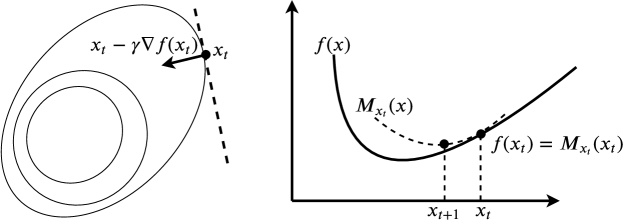
Figure 1.1: (Left) Illustration of gradient and steepest descent direction; (Right) Illustration of model function.

Minimizing a model function

Another perspective from which to view gradient descent is based on the model function. Since the original objective function $f({\bf x})$ is usually very complicated, it is very hard to minimize the objective function directly. A straightforward idea is to construct a model function to locally approximate (at ${\bf x}_{t}$) the original objective in each iteration. The model function needs to be simple and to approximate the original function well enough. Therefore, the most natural idea is to choose a quadratic function (that is usually simple to solve)

$$M_{{\bf x}_{t},\gamma}({\bf x}):=f({\bf x}_{t})+\langle f^{\prime}({\bf x}_{t}),{\bf x}-{\bf x}\rangle+{1\over 2\gamma}\|{\bf x}-{\bf x}_{t}\|^{2}.$$

This model function is a good approximation in the sense that

• $f({\bf x}_{t})=M_{{\bf x}_{t},\gamma}({\bf x}_{t})$

• $f^{\prime}({\bf x}_{t})=M^{\prime}_{{\bf x}_{t},\gamma}({\bf x}_{t})$

• $f(\cdot)\leq M_{{\bf x}_{t},\gamma}(\cdot)$ if the learning rate $\gamma$ is sufficiently small.

For the first two, it is easy to understand why they are important. The last one is important to the convergence, which will be seen soon. Figure 1.1 illustrates the geometry of the model function. One can verify that the GD algorithm is nothing but iteratively update the optimization variable ${\bf x}$ via minimizing the model function at the current point ${\bf x}_{t}$:

$${\bf x}_{t+1}= \operatorname*{argmin}_{{\bf x}}\leavevmode\nobreak\ M_{{\bf x}_{t},\gamma}({\bf x})$$

$$= \operatorname*{argmin}_{{\bf x}}\leavevmode\nobreak\ {1\over 2\gamma}\left\|{\bf x}-\left({\bf x}_{t}-\gamma f^{\prime}({\bf x}_{t})\right)\right\|^{2}+\text{constant}$$

$$= {\bf x}_{t}-\gamma f^{\prime}({\bf x}_{t}).$$

The convergence of GD can also be revealed by this intuition — ${\bf x}_{t+1}$ always improves ${\bf x}_{t}$ unless the gradient is zero

$$f({\bf x}_{t+1})\leq M_{{\bf x}_{t},\gamma}({\bf x}_{t+1})\leq M_{{\bf x}_{t},\gamma}({\bf x}_{t})=f({\bf x}_{t}),$$

where $f({\bf x}_{t=1})=f({\bf x}_{t})$ holds if and only if $f^{\prime}({\bf x}_{t})=0$.

1.1.2 Convergence rate

From the intuition of GD, the convergence of GD is automatically implied. This section provides the convergence rate via rigorous analysis. To show the convergence rate, let us first make some commonly used assumptions in the following.

The smoothness assumption on $F_{m}(\cdot)$’s implies that the overall objective function $f(\cdot)$ is differentiable or smooth too. The assumption (1.4) can be deduced from (1.3), and we refer readers to the textbook by boyd2004convex or their course link. The Lipschitz gradient assumption essentially assumes that the curvature of the objective function is bounded by $L$. We make the assumption of (1.4) just for convenience of use later.

We apply the Lipschitz gradient assumption and immediately obtain the following golden inequality:

$$f({\bf x}_{t+1})-f({\bf x}_{t})\leq \langle f^{\prime}({\bf x}_{t}),{\bf x}_{t+1}-{\bf x}_{t}\rangle+{L\over 2}\|{\bf x}_{t+1}-{\bf x}_{t}\|^{2}$$

$$= -\gamma\|f^{\prime}({\bf x}_{t})\|^{2}+{\gamma^{2}L\over 2}\|f^{\prime}({\bf x}_{t})\|^{2}$$

$$= -\gamma\left(1-{\gamma L\over 2}\right)\|f^{\prime}({\bf x}_{t})\|^{2}$$ (1.5)

We can see that as long as the learning rate $\gamma$ is small enough such that $1-{\gamma L}/2>0$, $f({\bf x}_{t+1})$ can improve $f({\bf x}_{t})$. Therefore, the learning rate cannot be too large to guarantee the progress in each step. However, it is also a bad idea if the learning rate is too small, since the progress is proportional to $\gamma(1-\gamma L/2)$. The optimal learning rate can be obtained by simply maximizing

$$\gamma(1-\gamma L/2)$$

over $\gamma$, which gives the optimal learning rate for the gradient descent method as $\gamma^{\star}=1/L$. Substituting $\gamma=\gamma^{\star}$ into (1.5) yields

$$f({\bf x}_{t+1})-f({\bf x}_{t})\leq-{1\over 2L}\|f^{\prime}({\bf x}_{t})\|^{2}$$

or equivalently

$$f({\bf x}_{t})-f({\bf x}_{t+1})\geq{1\over 2L}\|f^{\prime}({\bf x}_{t})\|^{2}.$$ (1.6)

Summarizing Eq. (1.6) over $t$ from $t=1$ to $t=T$ yields

$${1\over 2L}\sum_{t=1}^{T}\|f^{\prime}({\bf x}_{t})\|^{2}\leq \sum_{t=1}^{T}\left(f({\bf x}_{t})-f({\bf x}_{t+1})\right)$$

$$= f({\bf x}_{1})-f({\bf x}_{t+1})$$

$$\leq f({\bf x}_{1})-f^{\star}.$$

Rearranging the inequality yields the following convergence rate for gradient descent:

This result indicates that the averaged gradient norm converges in the rate of $1/T$. It is worth noting that, unlike the convex case, we are unable to use the commonly used criterion $f({\bf x}_{t})-f^{\star}$ to evaluate the convergence (efficiency). That is to say, the algorithm guarantees the convergence only to a stationary point ($\|f^{\prime}({\bf x}_{t})\|^{2}\rightarrow 0$) because of the nonconvexity. The connection between two criteria $f({\bf x}_{t})-f^{\star}$ and $\|f^{\prime}({\bf x}_{t})\|^{2}$ can be seen from

$${1\over L}\|f^{\prime}({\bf x}_{t})\|^{2}\leq f({\bf x}_{t})-f^{\star}.$$

The proof can be found in the standard textbook or the course link.

There are two major disadvantages for the GD method:

• The computational complexity and system overhead can be too high in each iteration to compute a single gradient;

• For nonconvex objectives, the gradient descent often sticks on a bad (shallow) local optimum.

1.1.3 Iteration / query / computation complexity

The convergence rate is the key to analyzing the overall complexity. People usually consider three types of overall complexity: iteration complexity, query complexity, and computation complexity. To evaluate the overall complexity to solve the optimization problem in (1.1), we need first to specify a precision of our solution, since in practice it is difficult (also not really necessary) to exactly solve the optimization problem. In particular, in our case the overall complexity must take into account how many iterations / queries / computations are required to ensure the average gradient norm ${1\over T}\sum_{t=1}^{T}\|f^{\prime}({\bf x}_{t})\|^{2}\leq\epsilon$.

Iteration complexity.

From Theorem 1.1.1, it is straightforward to verify that the iteration complexity is

$$O\left({L\over\epsilon}\right).$$ (1.8)

Query complexity.

Here “query” refers to the number of queries of the data samples. GD needs to query all $M$ samples in each iteration. Therefore, the query complexity can be computed from the iteration complexity by multiplying the number of queries in each iteration

$$O\left({LM\over\epsilon}\right).$$ (1.9)

Computation complexity.

Similarly, the computation complexity can be computed from the query complexity by multiplying the complexity of computing one sample gradient $F^{\prime}_{m}({\bf x})$. The typical complexity of computing one sample gradient is proportional to the dimension of the variable, which is $d$ in our notation. To see the reason, let us imagine a naive linear regression with $F_{m}:={1\over 2}({\bf a}_{m}^{\top}{\bf x}-b)^{2}$ and a sample gradient of $f^{\prime}_{m}({\bf x}):={\bf a}_{m}({\bf a}_{m}^{\top}{\bf x}-b)$. Therefore, the computation complexity of GD is

$$O\left({LMd\over\epsilon}\right).$$

It is worth pointing out that the computation complexity is usually proportional to the query complexity (no matter for what kinds of objective) if we consider and compare only first-order (or sample-gradient-based) methods. Therefore, in the remainder of this work, we compare only the query complexity and the iteration complexity.

1.2 Stochastic Gradient Descent

One disadvantage of GD is that it requires one to query all samples in an iteration, which could be overly expensive. To overcome this shortcoming, the stochastic gradient method SGD is widely used in machine learning training. Instead of computing a full gradient in each iteration, it is usual to compute only the gradient on a batch (or minibatch) of sampled data. In particular, people randomly sample an $m_{t}\in[M]$ independently each time and update the model by

$$(\texttt{SGD})\quad{\bf x}_{t+1}={\bf x}_{t}-\gamma F^{\prime}_{m_{t}}({\bf x}_{t}),$$ (1.10)

where $m_{t}\in[M]$ denotes the index randomly selected at the $t$th iteration. $F^{\prime}_{m}({\bf x})$ (or $F^{\prime}_{m_{t}}({\bf x}_{t})$) is called the stochastic gradient (at the $t$th iteration). We use ${\bf g}(\cdot):=F^{\prime}_{m}(\cdot)$ (or ${\bf g}_{t}(\cdot):=F^{\prime}_{m_{t}}(\cdot)$) to denote the stochastic gradient (or at the $t$th iteration) for short. An important property for the stochastic gradient is that its expectation is equal to the true gradient, that is,

$$\mathbb{E}[{\bf g}({\bf x})]=\mathbb{E}_{m}[F^{\prime}_{m}({\bf x})]=f^{\prime}({\bf x})\quad\forall{\bf x}.$$

An immediate advantage of SGD is that the computational complexity reduces to $O(d)$ per iteration. It is worth pointing out that the SGD algorithm is NOT a descent algorithm due to the randomness.

1.2.1 Convergence rate

The next questions are whether it converges and, if it does, how quickly. We first make a typical assumption:

We first apply the Lipschitzian gradient property in Assumption 1:

$$f({\bf x}_{t+1})-f({\bf x}_{t})\leq \langle f^{\prime}({\bf x}_{t}),{\bf x}_{t+1}-{\bf x}_{t}\rangle+{L\over 2}\|{\bf x}_{t+1}-{\bf x}_{t}\|^{2}$$

$$= -\gamma\langle f^{\prime}({\bf x}_{t}),{\bf g}_{t}({\bf x}_{t})\rangle+{L\gamma^{2}\over 2}\|{\bf g}_{t}({\bf x}_{t})\|^{2}.$$ (1.11)

Note two important properties:

• $\mathbb{E}[\langle f^{\prime}({\bf x}_{t}),{\bf g}_{t}({\bf x}_{t})\rangle]=\langle f^{\prime}({\bf x}_{t}),\mathbb{E}[{\bf g}_{t}({\bf x}_{t})]\rangle=\|f^{\prime}({\bf x}_{t})\|^{2}$

• $\mathbb{E}[\|{\bf g}_{t}({\bf x}_{t})\|^{2}]=\|f^{\prime}({\bf x}_{t})\|^{2}+\mathbb{E}[\|{\bf g}_{t}({\bf x}_{t})-f^{\prime}({\bf x}_{t})\|^{2}]\leq\|f^{\prime}({\bf x}_{t})\|^{2}+\sigma^{2}$,

where the second property uses the property of variance, that is, any random variable vector $\xi$ satisfies

$$\mathbb{E}[\|\xi\|^{2}]=\|\mathbb{E}[\xi]\|^{2}+\mathbb{E}[\|\xi-\mathbb{E}[\xi]\|]^{2}.$$ (1.12)

Apply these two properties to (1.11) and take expectation on both sides:

$$\mathbb{E}[f({\bf x}_{t+1})]-\mathbb{E}[f({\bf x}_{t})]$$

$$\leq -\gamma\mathbb{E}[\|f^{\prime}({\bf x}_{t})\|^{2}]+{L\gamma^{2}\over 2}\left(\mathbb{E}[\|f^{\prime}({\bf x}_{t})\|^{2}]+\sigma^{2}\right)$$ (1.13)

$$\leq -\gamma\left(1-{\gamma L\over 2}\right)\mathbb{E}[\|f^{\prime}({\bf x}_{t})\|^{2}]+{\gamma^{2}\over 2}L\sigma^{2}.$$ (1.14)

From (1.13), we can see that SGD does not guarantee “descent” in each iteration, unlike GD, but it does guarantee “descent” in the expectation sense in each iteration as long as $\gamma$ is small enough and $\|f^{\prime}({\bf x}_{t})\|^{2}>0$. This is because the first term in (1.13) is in the order of $O(\gamma)$ while the second term is in the order of $O(\gamma^{2})$.

Next we summarize (1.13) from $t=1$ to $t=T$ and obtain

$$\mathbb{E}[f({\bf x}_{T+1})]-f({\bf x}_{1})\leq-\gamma\left(1-{\gamma L\over 2}\right)\sum_{t=1}^{T}\mathbb{E}[\|f^{\prime}({\bf x}_{t})\|^{2}]+{\gamma^{2}\over 2}TL\sigma^{2}.$$ (1.15)

We choose the learning rate $\gamma={1\over L+\sigma\sqrt{TL}}$ which implies that $(1-\gamma L/2)>1/2$. It follows

$${1\over T}\sum_{t=1}^{T}\mathbb{E}[\|f^{\prime}({\bf x}_{t})\|^{2}]$$

$$\lesssim \frac{f({\bf x}_{1})-\mathbb{E}[f({\bf x}_{T+1})]}{T\gamma}+\gamma L\sigma^{2}$$

$$\lesssim \frac{f({\bf x}_{1})-f^{\star}}{T\gamma}+\gamma L\sigma^{2}$$

$$\lesssim {(f({\bf x}_{1})-f^{\star})L\over T}+{(f({\bf x}_{1})-f^{\star})\sqrt{L}\sigma\over\sqrt{T}}.$$

Therefore the convergence rate of SGD can be summarized into the following theorem

We highlight the following observations from Theorem 1.2.1

• (Consistent with GD) If $\sigma=0$, the SGD algorithm reduces to GD and the convergence rate becomes ${L(f({\bf x}_{1})-f^{\star})/L}$, which is consistent with the convergence rate for GD proven in Theorem 1.1.1.

• (Asymptotic convergence rate) The convergence rate of SGD achieves $O(1/\sqrt{T})$.

1.2.2 Iteration / query complexity

Using a similar analysis as Section 1.1.3, we can obtain the iteration complexity of SGD, which is also the query complexity (since there is only one query per one sample gradient)

$$O\left({L\over\epsilon}+{L\sigma^{2}\over\epsilon^{2}}\right).$$

It is worse than GD in terms of the iteration complexity in (1.8), which is not a surprising result. The comparison of query complexity makes more sense since it is more related to the physical running time or the computation complexity. From the detailed comparison in Table 1.2, we can see that

• SGD is superior to GD, if ${\sigma^{2}\over M}\ll\epsilon$;

• SGD is inferior to GD, if ${\sigma^{2}\over M}\gg\epsilon$.

It is worth pointing out that when the number of samples $M$ is huge and a low precision solution is satisfactory, ${\sigma\over M\sqrt{L}}\ll\epsilon$ usually holds. As a result, SGD is favored for solving big data problems.

algorithms	iteration complexity	query complexity
GD	$O\left({L\over\epsilon}\right)$	$O\left({ML\over\epsilon}\right)$
SGD	$O\left({L\over\epsilon}+{L\sigma^{2}\over\epsilon^{2}}\right)$	$O\left({L\over\epsilon}+{L\sigma^{2}\over\epsilon^{2}}\right)$
mb-SGD	$O\left({L\over\epsilon}+{L\sigma^{2}\over B\epsilon^{2}}\right)$	$O\left({LB\over\epsilon}+{L\sigma^{2}\over\epsilon^{2}}\right)$

Table 1.2: Complexity comparison among GD, SGD, and mb-SGD.

1.2.3 Minibatch stochastic gradient descent (mb-SGD)

A straightforward variant of the GD algorithm is to compute the gradient of a minibatch of samples (instead of a single sample) in each iteration, that is,

$${\bf g}^{\mathcal{B}}({\bf x})={1\over B}\sum_{m\in\mathcal{B}}F^{\prime}_{m}({\bf x}),$$ (1.16)

where $B:=|\mathcal{B}|$. The minibatch $\mathcal{B}$ is obtained by using i.i.d samples with (or without) replacement. One can easily verify that

$$\mathbb{E}[{\bf g}^{\mathcal{B}}({\bf x})]= f^{\prime}({\bf x}).$$

Sample “with” replacement.

The stochastic variance (for the “with” replacement case) can be bounded by

$$\mathbb{E}[\left\|{\bf g}^{\mathcal{B}}({\bf x})-f^{\prime}({\bf x})]\right\|^{2}]$$

$$= \mathbb{E}\left[\left\|{1\over B}\sum_{m\in\mathcal{B}}\left(F^{\prime}_{m}({\bf x})-f^{\prime}({\bf x})\right)\right\|^{2}\right]$$ (1.17)

$$= {1\over B}\sum_{m\in\mathcal{B}}\mathbb{E}\left[\left\|F^{\prime}_{m}({\bf x})-f^{\prime}({\bf x})\right\|^{2}\right]$$

$$\leq {\sigma^{2}\over B}\quad\left(\text{from Assumption\leavevmode\nobreak\ \ref{ass:sgd}}\right).$$

Sample “without” replacement

The stochastic variance for the “without” replacement is even smaller, but it involves a bit more complicated derivation. We essentially need the following key lemma

Proof 1.2.3.

First, it is not hard to see that the marginal distributions of $\xi_{m}$’s are identical. For simplicity of notation, we assume that $\mathbb{E}[\xi_{m}]=0$ without the loss of generality. Therefore, we have ${\bf Var}[\xi_{m}]=\mathbb{E}[\xi_{m}^{2}]$ for all $k$.

Next we have the following derivation:

$${\bf Var}[B\bar{\xi}_{[B]}]= \mathbb{E}[(B\bar{\xi}_{[B]})^{2}]\quad\text{(due to $\mathbb{E}[\bar{\xi}_{[B]}]=0$)}$$

$$= \sum_{m=1}^{B}\mathbb{E}[\xi_{m}^{2}]+\sum_{k\neq l}\mathbb{E}[\xi_{m}\xi_{l}]$$

$$= B{\bf Var}[\xi_{1}]+B(B-1)\mathbb{E}[\xi_{1}\xi_{2}],$$ (1.18)

where the last equality uses the fact $\mathbb{E}[\xi_{m}^{2}]={\bf Var}[\xi_{k}]={\bf Var}[\xi_{1}]$ for any $k$ and $E[\xi_{k}\xi_{l}]=E[\xi_{1}\xi_{2}]$ for any $k\neq l$. Note that ${\bf Var}[M\bar{\xi}_{[M]}]=0$, since it has only one possible combination for $\{\xi_{1},\xi_{2},\cdots,\xi_{M}\}$. Then letting $B=M$ obtains the following dependence from (1.18)

$$\mathbb{E}[\xi_{1}\xi_{2}]={-1\over M-1}{\bf Var}[\xi_{1}].$$

Plug this result into (1.18)

$${\bf Var}[B\bar{\xi}_{[B]}]=B\left({M-B\over M-1}\right){\bf Var}[\xi_{1}],$$

which implies the claimed result.

If $a_{m}$’s are vectors and satisfy ${1\over M}\sum_{m=1}^{M}\xi_{m}=0$, from Lemma 1.2.2 one can easily verify

$$\mathbb{E}\left[\|\bar{\xi}\|^{2}\right]=B\left({M-B\over M-1}\right)\mathbb{E}\left[\|\xi_{1}\|^{2}\right].$$ (1.19)

Now we are ready to compute the stochastic variance for the “without” replacement sampling strategy. Let $\mathcal{B}$ be a batch of samples “without” replacement. Then we let $\xi_{m}:=F^{\prime}_{m}({\bf x})-f^{\prime}({\bf x})$ and from (1.19) obtain

$$\mathbb{E}\left[\left\|{\bf g}^{\mathcal{B}}({\bf x})-f^{\prime}({\bf x})]\right\|^{2}\right]= \mathbb{E}\left[\|\bar{\xi}\|^{2}\right]$$

$$= \left({M-B\over M-1}\right){\mathbb{E}[\|\xi_{1}\|^{2}]\over B}$$

$$\leq \left({M-B\over M-1}\right){\sigma^{2}\over B}$$

$$\leq {\sigma^{2}\over B}.$$

To sum up, we have the stochastic variance bounded by ${\sigma^{2}\over B}$ no matter “with” or “without” replacement sampling.

We can observe that the effect of using a minibatch stochastic gradient is nothing but reduced variance. All remaining analysis for the convergence rate remains the same. Therefore, it is quite easy to obtain the convergence rate of mb-SGD

$${1\over T}\sum_{t=1}^{T}\mathbb{E}[\|f^{\prime}({\bf x}_{t})\|^{2}]\lesssim{L\over T}+{\sqrt{L}\sigma\over\sqrt{TB}}.$$ (1.20)

The iteration complexity and the query complexity are reported in Table 1.2.

1.3 A Simplified Distributed Communication Model

When scaling up the stochastic gradient descent (SGD) algorithm to a distributed setting, one often needs to develop system relaxations techniques to achieve better performance and scalability. In this work, we describe multiple popular system relaxation techniques that have been developed in recent years. In this section, we introduce a simple performance model of a distributed system, which will be used in later Sectionsto reason about the performance impact of different relaxation techniques.

From a mathematical optimization perspective, all of the system relaxations that we will describe do not make the convergence (loss vs. # iterations / epochs) faster. Then why do we even want to introduce these relaxations into our system in the first place?

One common theme of the techniques we cover in this work is that their goal is not to improve the convergence rate in terms of # iterations / epochs; rather, their goal is to make each iteration finish faster in terms of wall-clock time. As a result, to reason about each system relaxation technique in this work, we need to first agree on a performance model of the underlying distributed system. In this section, we introduce a very simple performance model — it ignores many (if not most) important system characteristics, but it is just informative enough for readers to understand why each system relaxation technique in this work actually makes a system faster.

1.3.1 Assumptions

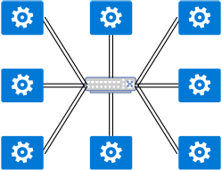
Figure 1.2: An illustration of the distributed communication model we use in this work. We assume that all devices (worker, machine) are connected via a “logical switch” whose property is defined in Section 1.3

.

In practice, it is often the case that the bandwidth or latency of each worker’s network connection is the dominating bottleneck in the communication cost. As a result, in this work we focus on the following simplified communication model.

Figure 1.2 illustrates our communication model. Each worker (blue rectangle) corresponds to one computation device (worker), and all workers are connected via a “logical switch” that has the following property:

1. The switch has infinitely large bandwidth. We make this simplifying assumption to reflect the observation that, in practice, the bottleneck is often the bandwidth or latency of each worker’s network connection.

2. For each message that “passes through” the switch (sent by worker $w_{i}$ and received by worker $w_{j}$), the switch adds a constant delay $t_{\text{latency}}$ independently of the number of concurrent messages that this switch is serving. This delay is the timestamp difference between the sender sending out the first bit and the receiver receiving the first bit.

For each worker, we also assume the following properties:

1. Each worker can only send one message at the same time.

2. Each worker can only receive one message at the same time.

3. Each worker can concurrently receive one message and send one message at the same time.

4. Each worker has a fixed bandwidth, i.e., to send / receive one unit (e.g., MB) amount of data, it requires $t_{\text{transfer1MB}}$ seconds.

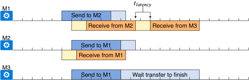
Figure 1.3: Illustration of the communication pattern of Example 1.3.2.

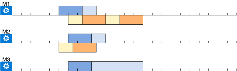
Figure 1.4: Illustration of the communication pattern of Example 1.3.2, with 2x data compression.

Example 1.3.1.

Under the above communication model, consider the following three events:

            time      event
            0:05      M1 send 1MB to M2
            0:06      M2 send 1MB to M1
            0:06      M3 send 1MB to M2

We assume that the latency added by the switch $t_{\text{latency}}$ is 1.5 units of time and it took 5 units of time to transfer 1MB of data. Figure 1.3 illustrates the timeline on three machines under our communication model. The yellow block corresponds to the latency added by the “logical switch”. We also see that the machine M1 can concurrently send (blue block) and receive (orange block) data at the same time; however, when the machine M3 tries to send data to M1, because the machine M2 is already sending data to M1, M3 needs to wait (the shallow blue block of M3).

Example 1.3.2.

Figure 1.4 illustrates a hypothetical scenario in which all data sent in Example 1.3.2 are “magically” compressed by 2$\times$ at the sender. As we will see in later Sections, this is similar to what would happen if one were to compress the gradient by 2$\times$ during training.

We make multiple observations from Figure 1.4.

1. First, compressing data does make the “system” faster. Without compression, all three events finish in 14 units of time (Figure 1.3) whereas it finishes in 9 units of time after compression. This is because the time used to transfer the data is decreased by half in our communication model.

2. Second, even if the data are compressed by 2$\times$, the speedup of the system is smaller than that; in fact, it is only $14/9=1.55\times$. This is because, even though the transfer time is cut by half, the communication latency does not decrease as a result of the data compression.

We now use the above communication model to describe the communication patterns of three popular ways to implement distributed stochastic gradient descent. These implementations will often serve as the baseline from which we apply different system relaxations to remove certain system bottlenecks that arise in different configurations of $(t_{\text{latency}},t_{\text{transfer}})$ together with the relative computational cost on each machine.

Workloads

We focus on one of the core building blocks to implement a distributed SGD system — each worker $M_{i}$ holds a parameter vector $w_{i}$, and they communicate to compute the sum of all parameter vectors: $S=\sum_{i}w_{i}$. At the end of communication, each worker holds one copy of $S$.

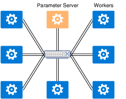
Figure 1.5: Illustration of the parameter server architecture with a single dedicated parameter server.

1.3.2 Synchronous Parameter Server

The parameter server is not only one of the most popular system architectures for distributed stochastic gradient descent; it is also one of the most popular communication models that researchers have in mind when they conduct theoretical analysis. In a parameter server architecture, one or more machines serve as the parameter server(s) and other machines serve as the workers processing data. Periodically, workers send updates to the parameters to the parameter servers and the parameter servers send back the updated parameters. Figure 1.5 illustrates this architecture: the orange machine is the parameter server and the blue machines are the workers.

A real-world implementation of a parameter server architecture usually involves many system optimizations to speed up the communication. In this section, we build our abstraction using the simplest implementation with only a single machine serving as the parameter server. We also scope ourselves and only focus on the synchronous communication case.

When using this simplified parameter server architecture to calculate the sum $S$, each worker $M_{i}$ sends their local parameter vector $w_{i}$ to the parameter server, and the parameter server collects all these local copies, sums them up, and sends back to each worker. In a simple example with three workers and one parameter server, the series of communication events looks like this:

        Time=0      Worker1 send w1 to PS
        Time=0      Worker2 send w2 to PS
        Time=0      Worker3 send w3 to PS
        Time=T      PS send S to Worker1
        Time=T      PS send S to Worker2
        Time=T      PS send S to Worker3

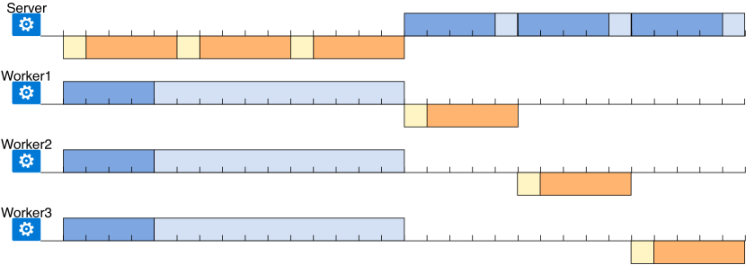
Figure 1.6: Illustration of the communication pattern of the parameter server architecture with a single dedicated parameter server.

Figure 1.6 illustrates the communication timeline of these events. We see that, in the first phase, all workers send their local parameter vectors to the parameter server at the same time. Because, in our communication model, the parameter server can receive data from only one worker at a time, it took $3(t_{\text{latency}}+t_{\text{transfer}})$ for the aggregation phase to finish. In the broadcast phase, because, in our communication model, the parameter server can send data to only one worker at a time, it took $3(t_{\text{latency}}+t_{\text{transfer}})$ for the broadcast phase to finish.

In general, when there are $N$ workers and $1$ parameter server, as under our communication model, a parameter server architecture in which all workers are perfectly synchronized takes

$$2N(t_{\text{latency}}+t_{\text{transfer}})$$

to compute and broadcast the sum $S$ over all local copies $\{w_{i}\}$.

Discussions

As we see, the communication cost of the parameter server architecture grows linearly with respect to the total number of workers we have in the system. As a result, this architecture could be sensitive to both latency and transfer time. This motivates some system relaxations that could alleviate potential system bottlenecks.

1. When the network has small latency $t_{\text{latency}}$ compared with the transfer time $t_{\text{transfer}}$, one could conduct lossy compression (e.g., via quantization, sparsification, or both) to decrease the transfer time. Usually, this approach can lead to a linear speedup with respect to the compression rate, up to a point that $t_{\text{latency}}$ starts to dominate.

2. When the network has large latency $t_{\text{latency}}$, compression on its own won’t be the solution. In this case, one could adopt a decentralized communication pattern, as we will discuss later in this work.

1.3.3 AllReduce

Calculating the sum over distributed workers is a very common operator used in distributed computing and high performance computing systems. In many communication frameworks, it can be achieved using the AllReduce operator. Optimizing and implementing the AllReduce operator has been studied by the HPC community for decades, and the implementation is usually different for different numbers of machines, different sizes of messages, and different physical communication topologies.

In this work, we focus on the simplest case, in which all workers form a logical ring and communicate only to their neighbors (all communications still go through the single switch all workers are connected to). We also assume that the local parameter vector is large enough.

Under these assumptions, we can implement an AllReduce operator in the following way. Each worker $w_{n}$ partitions their local parameter vectors into $N$ partitions ($N$ is the number of workers): $w_{n}^{k}$ is the $k$th partition of the local model $w_{n}$. The communication happens in two phases:

1. Phase 1. At the first iteration of Phase 1, each machine $n$ sends $w_{n}^{n}$ to its “next” worker in the logical ring, i.e., $w_{j}$ where $j=n+1\mod N$. Once machine $j$ receives a partition $k$, it sums up the received partition with its local partition, and sends the aggregated partition to the next worker in the next iteration. After $N-1$ communication iterations, different workers now have the sum of different partitions.

2. Phase 2. Phase 2 is similar to Phase 1, with the difference that when machine $n$ receives a partition $k$, it replaces its local copy with the received partition, and passes it onto the next machine in the next iteration.

At the end of communication, all workers have the sum $S$ of all partitions.

Example 1.3.3.

We walk through an example with four workers $M_{1}$, … $M_{4}$. The communication pattern of the above implementation is as follows. We use w{Mi,j} to denote the $j$th partition on machine Mi.

# For the first partition w{M1 (worker id), 1 (partition id)}
Time= 0   M1 sends w{M1,1}                               to M2
Time= t   M2 sends w{M1,1} + w{M2,1}                     to M3
Time=2t   M3 sends w{M1,1} + w{M2,1} + w{M3,1}           to M4
Time=3t   M4 sends w{M1,1} + w{M2,1} + w{M3,1} + w{M4,1} to M1
Time=4t   M1 sends w{M1,1} + w{M2,1} + w{M3,1} + w{M4,1} to M2
Time=5t   M2 sends w{M1,1} + w{M2,1} + w{M3,1} + w{M4,1} to M3

# For the second partition w{M2 (worker id), 2 (partition id)}
Time= 0   M2 sends w{M2,2}                               to M3
Time= t   M3 sends w{M2,2} + w{M3,2}                     to M4
Time=2t   M4 sends w{M2,2} + w{M3,2} + w{M4,2}           to M1
Time=3t   M1 sends w{M2,2} + w{M3,2} + w{M4,2} + w{M1,2} to M2
Time=4t   M2 sends w{M2,2} + w{M3,2} + w{M4,2} + w{M1,2} to M3
Time=5t   M3 sends w{M2,2} + w{M3,2} + w{M4,2} + w{M1,2} to M4

# For the third partition w{M3 (worker id), 3 (partition id)}
Time= 0   M3 sends w{M3,3}                               to M4
Time= t   M4 sends w{M3,3} + w{M4,3}                     to M1
Time=2t   M1 sends w{M3,3} + w{M4,3} + w{M1,3}           to M2
Time=3t   M2 sends w{M3,3} + w{M4,3} + w{M1,3} + w{M2,3} to M3
Time=4t   M3 sends w{M3,3} + w{M4,3} + w{M1,3} + w{M2,3} to M4
Time=5t   M4 sends w{M3,3} + w{M4,3} + w{M1,3} + w{M2,3} to M1

# For the fourth partition w{M4 (worker id), 4 (partition id)}
Time= 0   M4 sends w{M4,4}                               to M1
Time= t   M1 sends w{M4,4} + w{M1,4}                     to M2
Time=2t   M2 sends w{M4,4} + w{M1,4} + w{M2,4}           to M3
Time=3t   M3 sends w{M4,4} + w{M1,4} + w{M2,4} + w{M3,4} to M4
Time=4t   M4 sends w{M4,4} + w{M1,4} + w{M2,4} + w{M3,4} to M1
Time=5t   M1 sends w{M4,4} + w{M1,4} + w{M2,4} + w{M3,4} to M2

From the above pattern, it is not hard to see why, at the end, each worker has a copy of $S=\sum_{n=1}^{N}w_{n}$.

Figure 1.7: Illustration of the communication pattern of the AllReduce architecture with ring topology.

One interesting property of the above way of implementing the AllReduce operator is that, at any timestep, each machine concurrently sends and receives one partition of the data, which is possible in our communication model. Figure 1.7 illustrates the communication timeline.

We make multiple observations.

1. Compared with a parameter server architecture with a single parameter server (Figure 1.6), the total amount of data that each worker sends and receives is the same in both cases — in both cases, the amount of data sent and received by each machine is equal to the size of the parameter vector.

2. At any given time, each worker sends and receives data concurrently. At any given time, only the left neighbor $w_{n}$ sends data to $w_{n+1\mod N}$ and $w_{n+1\mod N}$ only sends data to $w_{n+2\mod N}$. This allows the system to take advantage of the aggregated bandwidth of $N$ machines (which grows linearly with respect to $N$) instead of being bounded by the bandwidth of a single central parameter server.

In general, when there are $N+1$ workers, as under our communication model and assuming that the computation cost to sum up parameter vectors is negligible, an AllReduce operator in which all workers are perfectly synchronized took

$$2Nt_{\text{latency}}+2t_{\text{transfer}}$$

to compute and broadcast the sum $S$ over all local copies $\{w_{n}\}$.

Discussions

As we see, the latency of an AllReduce operator grows linearly with respect to the total number of workers we have in the system. As a result, this architecture could be sensitive to network latency. This motivates some system relaxations that could alleviate potential system bottlenecks.

1. When the network has large latency $t_{\text{latency}}$, compression on its own won’t be the solution. In this case, one could adopt a decentralized communication pattern, as we will discuss later in this work.

2. When the network has small latency $t_{\text{latency}}$ and the parameter vector is very large, the transfer time $t_{\text{transfer}}$ can still become the bottleneck. In this case, one could conduct lossy compression (e.g., via quantization, sparsification, or both) to decrease the transfer time. Usually, this approach can lead to a linear speedup with respect to the compression rate, up to a point that $t_{\text{latency}}$ starts to dominate.

Caveats

We will discuss the case of asynchronous communication later in this work. Although it is quite natural to come up with an asynchronous parameter server architecture, making the AllReduce operator run in an asynchronous fashion is less natural. As a result, when there are stragglers in the system (e.g., one worker is significantly slower than all other workers), AllReduce can make it more difficult to implement a straggler avoidance strategy if one simply uses the off-the-shelf implementation.

Why Do We Partition the Parameter Vector?

One interesting design choice in implementing the AllReduce operator is setting each local parameter vector to be partitioned into $N$ partitions. This decision is important if you want to fully take advantage of the aggregated bandwidth of all workers. Take the same four-worker example and assume that we do not partition the model. In this case, the series of communication events will look like this:

Time= 0   M1 sends w{M1}                         to M2
Time= t   M2 sends w{M1} + w{M2}                 to M3
Time=2t   M3 sends w{M1} + w{M2} + w{M3}         to M4
Time=3t   M4 sends w{M1} + w{M2} + w{M3} + w{M4} to M1
Time=4t   M1 sends w{M1} + w{M2} + w{M3} + w{M4} to M2
Time=5t   M2 sends w{M1} + w{M2} + w{M3} + w{M4} to M3

In general, with $N+1$ workers, the communication cost without partitioning becomes

$$2N(t_{\text{latency}}+t_{\text{transfer}}).$$

Comparing this with the $2Nt_{\text{latency}}+2t_{\text{transfer}}$ cost of AllReduce with model partition, we see that model partition is the key reason for taking advantage of the full aggregated bandwidth provided by all machines.

1.3.4 Multi-machine Parameter Server

One can extend the single-server parameter server architecture and use multiple machines serving as parameter servers instead. In this work, we focus on the scenario in which each worker also serves as a parameter server.

Under this assumption, we can implement a multi-server parameter server architecture in the following way. Each worker $w_{n}$ partitions their local parameter vectors into $N$ partitions ($N$ is the number of workers): $w_{n}^{k}$. The communication happens in two phases:

1. Phase 1: All workers send their $n^{th}$ partition to worker $w_{n}$. Worker $w_{n}$ aggregates all messages and calculates the $n^{th}$ partition of the sum $S$.

2. Phase 2: Worker $w_{n}$ sends the $n^{th}$ partition of the sum $S$ to all other workers.

With careful arrangement of communication events, we can also take advantage of the full aggregated bandwidth in this architecture, as illustrated in the following example.

Example 1.3.4.

We walk through an example with four workers $M_{1}$, … $M_{4}$. The communication pattern of the above implementation is as follows:

# First partition: w{M1 (worker id), 1 (partition id)}
# First partition of the result: S{1}
Time= 0   M2 sends w{M2,1} to M1
Time= t   M3 sends w{M3,1} to M1
Time=2t   M4 sends w{M4,1} to M1
Time=3t   M1 sends S{1}    to M2
Time=4t   M1 sends S{1}    to M3
Time=5t   M1 sends S{1}    to M4

# Second partition: w{M2 (worker id), 2 (partition id)}
# Second partition of the result: S{2}
Time= 0   M1 sends w{M1,2} to M2
Time= t   M4 sends w{M4,2} to M2
Time=2t   M3 sends w{M3,2} to M2
Time=3t   M2 sends S{2}    to M3
Time=4t   M2 sends S{2}    to M4
Time=5t   M2 sends S{2}    to M1

# Third partition w{M3 (worker id), 3 (partition id)}
# Third partition of the result: S{3}
Time= 0   M4 sends w{M4,3} to M3
Time= t   M1 sends w{M1,3} to M3
Time=2t   M2 sends w{M2,3} to M3
Time=3t   M3 sends S{3}    to M4
Time=4t   M3 sends S{3}    to M1
Time=5t   M3 sends S{3}    to M2

# Fourth partition w{M4 (worker id), 4 (partition id)}
# Fourth partition of the result: S{4}
Time= 0   M3 sends w{M3,4} to M4
Time= t   M2 sends w{M2,4} to M4
Time=2t   M1 sends w{M1,4} to M4
Time=3t   M4 sends S{4}    to M1
Time=4t   M4 sends S{4}    to M2
Time=5t   M4 sends S{4}    to M3

For the above communication events, it is not hard to see that, at the end, each machine has access to the sum $S=\sum_{n=1}^{N}{w_{n}}$. In terms of the communication pattern, under our communication model, the multi-server parameter server architecture has the same pattern as AllReduce, illustrated in Figure 1.7.

In general, when there are $N+1$ workers, as under our communication model and assuming that the computation cost to sum up parameter vectors is negligible, a multi-server parameter server architecture in which all workers are perfectly synchronized took

$$2Nt_{\text{latency}}+2t_{\text{transfer}}$$

to compute and broadcast the sum $S$ over all local copies $\{w_{n}\}$.

Chapter 2 Distributed Stochastic Gradient Descent

The previous Sectionprovides us with the background of stochastic gradient descent and a simple communication model. This allows us to start analyzing the performance of a simple, distributed stochastic gradient descent system, which will serve as the baseline for the remaining part of this work.

2.1 A Simplified Performance Model for Distributed Synchronous Data-Parallel SGD

Recall the optimization problem that we hope to solve:

$$\min_{{\bf x}\in\mathbb{R}^{d}}\quad\left\{f({\bf x}):={1\over M}\sum_{m=1}^{M}F_{m}({\bf x})\right\}$$ (2.1)

The stochastic gradient descent algorithm works by sampling, uniformly randomly with replacement, a term $m_{t}\in[M]$, and updating the current model ${\bf x}_{t}$ with

$${\bf x}_{t+1}={\bf x}_{t}-\gamma F^{\prime}_{m_{t}}({\bf x}_{t})$$

until convergence.

Figure 2.1: Illustration of SGD on a single machine.

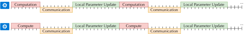
Figure 2.2: Illustration of the distributed synchronous data-parallel SGD.

2.1.1 SGD on a Single Machine

Implementing SGD on a single machine, with a single thread, is easy. The system stores the current model ${\bf x}_{t}$ in memory, and repeats two stages, as illustrated in Figure 2.1:

1. Computation: The system (1) fetches ${\bf x}_{t}$ from the main memory; (2) fetches all information necessary to compute $F_{m_{t}}^{\prime}({\bf x}_{t})$; and (3) computes $F_{m_{t}}^{\prime}({\bf x}_{t})$.

2. Update: The system updates ${\bf x}_{t}$ with $F_{m_{t}}^{\prime}({\bf x}_{t})$.

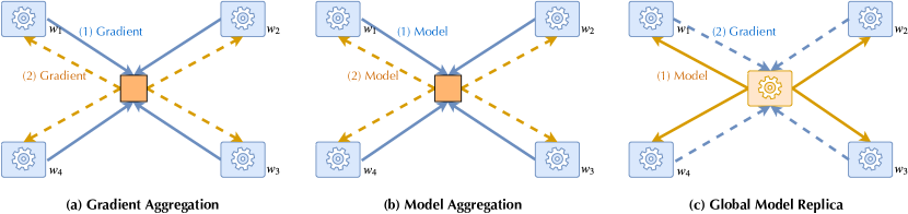
Figure 2.3: Illustration of three possible implementations of data-parallel SGD on multiple devices.

2.1.2 Data-Parallel SGD on Multiple Devices

When distributing the above algorithm on multiple devices, there are multiple ways of distributing the workload for different system bottlenecks. For example, when the model ${\bf x}_{t}$ is too large and does not fit into the fast memory of a single device, it can be partitioned onto different devices for the computation phase. This strategy is called model parallelism. In this work, we focus on what is called data parallelism — each device has access to a partition of the data set (i.e., $[M]$), and repeats a three-stage process as illustrated in Figure 2.2.

1. Computation: Each worker (say worker $n$) samples, from its local partition, an $F_{m_{t}^{(n)}}^{\prime}({\bf x}_{t})$ to compute. $m_{t}^{(n)}$ denotes the index sampled by worker $n$ at iteration $t$.

2. Communication: Workers communicate to compute the sum of all local gradients $\sum_{n}F_{m_{t}^{(n)}}^{\prime}({\bf x}_{t})$.

3. Update: The system updates ${\bf x}_{t}$ with $\sum_{n}F_{m_{t}^{(n)}}^{\prime}({\bf x}_{t})$.

The above algorithm can be implemented in three ways, depending on whether the system aggregates the gradient or the model, and the locality of model. Figure 2.3 illustrates these three implementations.

Gradient Aggregation

One simple strategy to implement the above algorithm is for each worker $w_{n}$ to maintain a local model replica ${\bf x}_{t}^{(n)}$. At the very beginning, the replica on all workers is the same:

$${\bf x}_{0}^{(1)}=\cdots={\bf x}_{0}^{(N)}.$$

In the communication phase, the system aggregates the gradient using any one of the three communication primitives we introduced before (e.g., AllReduce). At the end of communication, each worker sees the same aggregated gradient

$$\sum_{n}F_{m_{t}^{(n)}}^{\prime}({\bf x}_{t}).$$

In the update phase, each worker applies the update locally, independently. Because all workers see the same aggregated gradient, their model replica stays equal after the updates.

Model Aggregation

It is possible to implement the system in a different way. Each worker $w_{n}$ still maintains the local replica ${\bf x}_{t}^{(n)}$ and makes sure they are the same at the very beginning.

However, the system does the local update first by applying the local gradient to each local model:

$${\bf x}_{t+1/2}^{(n)}={\bf x}_{t}^{(n)}-\gamma F_{m_{t}^{(n)}}^{\prime}({\bf x}_{t}^{(n)})$$

In the communication phase, all workers communicate the model, $x_{t+1/2}^{(n)}$ and calculate the sum

$${\bf x}_{t+1}={1\over N}\sum_{n}{\bf x}_{t+1/2}^{(n)}={\bf x}_{t}-\gamma{1\over N}\sum_{n}F_{m_{t}^{(n)}}^{\prime}({\bf x}_{t}^{(n)})$$

The system then uses this sum ${\bf x}_{t+1}$ to update its local model replica.

Global Model Replica

The third way of implementing the system is to maintain a global, instead of local, model replica. This global replica is stored on one, or multiple, parameter servers. At the very beginning, each worker $w_{j}$ fetches the global model replica ${\bf x}_{t}$ from the parameter servers, calculates the local gradient, and sends the local gradient to the parameter servers. The parameter server then calculates the sum of all local gradients, and updates its global replica.

Discussion

It is easy to see that all three implementations logically implement the same algorithm. However, the system tradeoff among these three different implementations can be quite delicate.

1. Size of Model $=$ Size of Gradient. When the size of the model is the same as the size of the gradient, these three implementations can have similar communication cost. When we implement the gradient aggregation and model aggregation approach using AllReduce and the global model replica using a multi-server parameter server, we see that all three implementations have the communication cost

   $$2Nt_{\text{latency}}+2t_{\text{transfer}}$$

   where the transfer time $t_{\text{transfer}}$ depends only on the size of the model and the gradient. In this case, we would expect the end-to-end performance of these three implementations to be similar.

2. Size of Model $\neq$ Size of Gradient. The tradeoff between these three implementations becomes more complex when the size of the model does not equal the size of the gradient. For example, there could be a very dense model but a very sparse gradient, or vice versa. When this happens, these three implementations can have very different performance. Specifically, the communication cost can be summarized as follows:

   1. Gradient Aggregation (AllReduce):

      $$2Nt_{\text{latency}}+2t_{\text{transfer}}^{(\text{grad})};$$

   2. Model Aggregation (AllReduce):

      $$2Nt_{\text{latency}}+2t_{\text{transfer}}^{(\text{model})};$$

   3. Global Model Replica (Multi-server PS):

      $$2Nt_{\text{latency}}+t_{\text{transfer}}^{(\text{model})}+t_{\text{transfer}}^{(\text{grad})}.$$

   Obviously, different applications can have different performance under these three implementations.

In this work, we assume that the size of the model and the size of the gradient are always the same. Readers might wonder why we bother to introduce all three strategies, given that they all have similar performance under this assumption. As we will see later, different types of system relaxations might be more suitable to be applied to different implementations. For example, asynchronous relaxation might be easier to implement when there is a global model replica. Moreover, some system relaxations might require different theoretical analysis under different implementations. For example, the lossy quantization technique applied to gradient aggregation and model aggregation lead to different convergence behavior; decentralized relaxation might not work at all if one uses gradient aggregation.

In this work, when introducing different system relaxations, we assume that we have the luxury of choosing one from these three implementations without worrying about the delicate tradeoff between them. In practice, given a specific type of ML models, choosing the right implementation and system relaxation is often an engaged, task-specific problem.

2.2 Theoretical Analysis

The theoretical analysis is very similar to the mb-SGD we introduced in Section 1.2.3. One can simply imagine that the minibatch stochastic gradient in (1.16) is computed by $N$ workers and that the minibatch size is $N=B$. Then, the convergence rate can be easily obtained from (1.20)

$${1\over T}\sum_{t=1}^{T}\mathbb{E}[\|f^{\prime}({\bf x}_{t})\|^{2}]\lesssim{L\over T}+{\sqrt{L}\sigma\over\sqrt{TN}}.$$ (2.2)

2.3 Caveats

These are multiple aspects of data-parallel SGD implementations that we will not consider in this work. These aspects are often critical in practice to achieving good performance; however, including them into theoretical analysis is either impossible (because of the lack of an analytical understanding) or more engaged (because of the sophisticated performance model introduced by these factors). The goal of this work is not to cover all aspects of distributed learning; instead, providing a minimalist tutorial of the basics. As a result, we briefly discuss these aspects. We refer readers to Section 6 for further reading about these topics.

1. Batch size. One aspect that we do not consider in our analysis is the impact of batch size on model accuracy. The underlying assumption of this work is that using a larger batch size, once converged, will lead to the same model accuracy as a smaller batch size. This assumption allows us to treat the impact of larger batch size as a way to reduce the variance of the stochastic gradient. However, in practice, especially for models such as deep neural networks, the impact of batch size can be quite delicate and could also have an impact on accuracy and generalization.

2. Hardware parallelism. Another assumption that we are making on the system side is that the time that one device needs to compute stochastic gradient over one data point is $K$ times cheaper than computing stochastic gradient over a batch of $K$ data points. This is true in terms of the number of floating point operations that one needs to conduct; however, it might not necessarily be true with real-world hardware in terms of wall-clock time. For hardware, especially those optimizing throughput such as GPUs, batching might have a significant impact on performance. In some cases, calculating a single data point might be as expensive as processing a batch of data points, in terms of wall-clock time. This aspect, together with the impact of batch size on model accuracy, could make it quite complicated to design distributed learning systems.

3. Model structure. In this work, we assume that the model (${\bf x}_{t}$) is a dense vector that does not have much structure. In practice, the model might have more structures. For example, if ${\bf x}_{t}$ corresponds to a deep neural network, it can be decomposed into multiple layers. If one uses the standard back-propagation algorithm, the communication of layer can be overlapped with the computation (e.g., one can calculate the gradient of layer $l$ when communicating for layer $l+1$ in the backward pass). Recent research has tried to take advantage of this structure (See Section 6). As another example, when the data or model has some sparsity structure, one could also take advantage of it during (distributed) training.

4. Communication Model. Last but not least, we assume that communication via the “logical switch” is the only way that different devices can communicate. However, in practice, modern hardware is more complicated than this — different CPU cores might “communicate” via the shared L3 cache; different CPU sockets might “communicate” via QPI; a GPU/CPU hybrid system has even more delicate ways of communicating. Designing a distributed learning system when each of the workers is a multi-socket CPU system together with multiple GPU devices is more complicated than the simple performance model that we cover in this work.

Chapter 3 System Relaxation 1: Lossy Communication Compression

In distributed systems, data movement can often be significantly slower than computation. This is also often true for distributed learning — a forward and backward pass to calculate the gradient on a 152-layer ResNet requires roughly 3 $\times$ 11 GFLOPS and has a 230 MB model. In theory, with 16 GPUs, each of which provides 10 TFLOPS, and a 40 Gbit network, a 256-image batch would require 0.05 seconds for gradient calculation, but would require 0.09 seconds for network transfer time. In practice, both processes are often slower than the theoretical peak; however, their relative order remains similar.

In this Section, we focus on one system relaxation technique to speed up the expensive gradient exchange step in distributed SGD — instead of exchanging the gradient as 32bit floating point numbers, the system first quantizes it into a lower precision representation before communication. The impact of this relaxation is to decrease the time needed to transfer a model — if one quantizes the gradient into 8bit fixed point representation, the transfer time would theoretically decrease by 4$\times$.

3.1 System Implementation

To implement this system relaxation, two aspects of the process need to be addressed.

1. How can a floating point vector ${\bf x}$, representing either the model or the gradient, be compressed, using a function $Q(\cdot)$ such as the result $Q({\color[rgb]{0,0,0}})$, which can be stored more efficiently (either more sparsely than ${\bf x}$ via sparsification, or using fewer bits via quantization)?

2. How can the lossy compression function $Q(-)$ be used to implement distributed SGD? As we will see later, compressing different communication channels for different implementations of distributed SGD (i.e., model aggregation, gradient aggregation, and a global model replica) actually leads to different algorithms and needs different analysis of convergence.

3.1.1 Lossy Communication Compression

There are multiple ways of conducting lossy compression that are popularly used for distributed SGD. In this work, we focus on unbiased lossy compression, which ensures that

$$\mathbb{E}_{\xi}\left[Q({\color[rgb]{0,0,0}};\xi)\right]={\color[rgb]{0,0,0}}.$$

The term $\xi$ denotes the randomness of compression, and the above equation ensures that the compressed vector $Q({\color[rgb]{0,0,0}};\xi)$ is unbiased with respect to the original vector $x$.

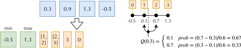
Figure 3.1: Illustration of One Simple Quantization Method.

Unbiased Compression via Quantization

There are multiple ways of conducting unbiased compression, and quantization is arguably the simplest approach. Figure 3.1 illustrates this process.

Given an original input vector ${\bf x}$, stored as floating points (e.g., 32 bits per element), let $\min({\bf x})$ and $\max({\bf x})$ be the smallest and the largest element of ${\bf x}$. A simple way of quantizing the input vector using $b$-bits per element is simply to quantize each element of ${\bf x}$, ${\bf x}_{i}$ independently. With $b$-bits, one can represent $2^{b}$ “knobs” partitioning the range $[\min({\bf x}),\max({\bf x})]$. Assume these knobs are uniformly located as $\{c_{0},...,c_{2^{b}-1}\}$, i.e.,

$$c_{i}=i\times\frac{\max({\bf x})-\min({\bf x})}{2^{b}-1}+\min({\bf x}).$$

Assume that the $i^{th}$ element of ${\bf x}$, ${\bf x}_{i}$ falls between $[c_{i},c_{i+1})$; we can use the following randomized quantization (RQ) function:

$$Q({\bf x}_{i};\xi_{i})=\left\{\begin{array}[]{c}c_{i}\leavevmode\nobreak\ \leavevmode\nobreak\ \leavevmode\nobreak\ \leavevmode\nobreak\ \leavevmode\nobreak\ \leavevmode\nobreak\ \leavevmode\nobreak\ \xi>\frac{{\bf x}_{i}-c_{i}}{c_{i+1}-c{i}}\\ c_{i+1}\leavevmode\nobreak\ \leavevmode\nobreak\ \leavevmode\nobreak\ \leavevmode\nobreak\ \leavevmode\nobreak\ \text{otherwise}\end{array}\right.$$ (3.3)

where $\xi_{i}$ is a uniform random variable on $[0,1]$.

Figure 3.1 illustrates this process for $b=2$ (i.e., 2-bit per element) and $\min({\bf x})=-0.5,\max({\bf x})=1.3$. Take the first element $0.3$, for example: it falls in the internal $[0.1,0.7)$. As a result, with probability $\frac{2}{3}$ the system quantizes the element 0.3 to 0.1 and with probability $\frac{1}{3}$, the system quantizes the element 0.3 to 0.7. If one calculates the expectation, we have

$$\frac{2}{3}\times 0.1+\frac{1}{3}\times 0.7=0.3$$

Because there are only $2^{b}$ knobs that the quantization function $Q(-)$ can take values in, the output can be encoded using $b$ bits per element.

Caveats

The above approach is one of the simplest ways to construct an unbiased compression function. There are multiple ways that it can be improved. We briefly summarize these caveats below and refer readers to Section 6 for further readings.

1. In practice, more sophisticated quantization functions can be constructed. For example, instead of normalizing the vector using $l_{\infty}$ norm (i.e., $\min({\bf x}),\max({\bf x})$), one can normalize it using other norms, say $l_{2}$. One can also partition the vectors into different “buckets” and quantize each bucket independently. Moreover, the “knobs” do not need to be uniformly distributed over $[\min({\bf x}),\max({\bf x})]$, and one can even learn those knobs as part of the learning process. All these approaches have been used for communication quantization and can sometimes outperform the baseline quantization strategy that we just introduced.

2. If the original input vector is stored as 32-bit floating point numbers, quantization can only provide at most 32$\times$ compression, because one cannot compress each element below a single bit. There are other approaches that do not have this limitation. One such approach is called sparsification, which maps the input vector $x$ to another vector $x^{\prime}$ that is more sparse. This mapping can also be made to be unbiased, a strategy that has been popular in practice.

3. In this work, we focus on the scenario in which the lossy compression scheme is unbiased. However, a biased compression scheme can still be used while still achieving convergence of the training process. For example, a vector ${\bf x}$ can be compressed by taking the top-$k$ element. This operation is clearly biased, but there is recent work proving convergence using this type of biased compression scheme.

3.1.2 SGD with Lossy Communication Compression (CSGD)

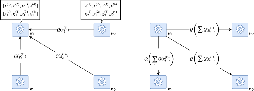
Figure 3.2: Illustration of Multi-server Parameter Servers with Lossy Communication Compression. In this example, there are four workers. Each worker is the parameter server of one partition of the model. This figure illustrates the communication for the first partition of the model $x^{(1)}$ hosted by the first worker $w_{1}$.

It is possible to use a quantization function $Q(-)$ to compress communications for distributed training. In the previous Sections, we described three different ways of implementing distributed SGD and different communication primitives; for each of these implementations and primitives, compressing the communication might actually lead to different algorithms and convergence behaviors.

Multi-server Parameter Server for Gradient Aggregation

The easiest implementation for demonstrating the impact of lossy compression is probably gradient aggregation using a multi-server parameter server. In this strategy, each machine holds a replica of the full model. Given $N$ machines, the gradient vector is partitioned into $N$ chunks — each machine $w_{n}$ is responsible for aggregating the $n^{th}$ partition, as illustrated in Figure 3.2.

Specifically, all machines send their $n^{th}$ partition of the local gradient to the worker $w_{n}$, which aggregates all incoming vectors and broadcasts back the sum. Both the incoming and outcoming messages can be compressed by using the quantization function. Let the local gradient on worker $n$ be $g_{n}$; after aggregation, each worker receives

$$Q\left({1\over N}\sum_{n=1}^{N}Q(g_{n})\right).$$ (3.4)

AllReduce for Gradient Aggregation

Figure 3.3: Illustration of AllReduce with Lossy Communication Compression. In this example, there are four workers. Each worker initiates the communication of one partition of the model. This figure illustrates the communication for the first partition of the model $x^{(1)}$ initiated by the first worker $w_{1}$.

We can also apply lossy compression to AllReduce, which makes the system behavior more complicated to analyze. Figure 3.3 illustrates the communication pattern.

Specifically, given $n$ workers, the system divides the local gradient into $n$ partitions. Each partition “flows through” a ring formed by all the machines, and keeps getting aggregated with the local gradient (Figure 3.3(left)). At the end, one worker has the result of the aggregation. In the second step, the aggregated result “flows through” a ring of all the machines again — whenever a machine receives the aggregated result, it makes a local copy, and sends the aggregated result to the next machine in the ring (Figure 3.3(left)).

One caveat of this strategy is that, in order to make sure all incoming and outcoming messages are compressed, the sum must be compressed $N$ times if there are $N$ machines in the ring. As a result, as illustrated in Figure 3.3, after aggregation, each worker receives

$$Q(\cdots Q(Q(Q(Q(Q(g_{1})+g_{2})+g_{3})+g_{4})\cdots+g_{N}).$$ (3.5)

Compared with the aggregated result in the parameter server case ($Q({1\over N}\sum_{n=1}^{N}Q(g_{n}))$), it is clear that the AllReduce case requires more engaged analysis.

Impact of Lossy Compression

Figure 3.4: Illustration of the Impact of Lossy Compression (Without Compression)

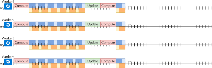
Figure 3.5: Illustration of the Impact of Lossy Compression (With 2$\times$ Compression)

Both implementations have a similar impact on the end-to-end performance. Figure 3.4 and Figure 3.5 illustrate the impact of a 2$\times$ compression.

We see that lossy compression would decrease the transfer time, as the communicated messages are now smaller. It does not have any impact on latency, as the number of communications the system needs to conduct stays the same. In this example, we ignore the computation cost of conducting the compression, which is often small compared with the computation time of the gradient.

Specifically, for AllReduce and a multi-server parameter server whose communication cost is

$$2nt_{\text{latency}}+2t_{\text{transfer}},$$

compressing the communication by $K$ times leads to a communication cost of

$$2nt_{\text{latency}}+\frac{2}{K}t_{\text{transfer}}.$$

When system performance is bounded by the communication cost, and the communication cost is dominated by the transfer time, we observe linear speedup with respect to the compression ratio, in terms of the time needed to finish a single iteration.

3.2 Theoretical Analysis for CSGD

In this section, we analyze CSGD, an SGD  variant in which the stochastic gradient is compressed by some lossy compression scheme. The analysis for the CSGD algorithm is very similar to the analysis for stochastic gradient based methods we have seen in previous Sections. First, we can see that the basic updating rule for CSGD is nothing but

$${\bf x}_{t+1}={\bf x}_{t}-\gamma{\bf g}_{t},$$ (3.6)

where ${\bf g}_{t}$ could take the form of either (3.4) or (3.5). But it needs to admit the following two key assumptions, which essentially serve the same purpose as as Assumption 2:

• (Unbiased gradient) The stochastic gradient is unbiased, that is,

  $$\mathbb{E}[{\bf g}_{t}]=f^{\prime}({\bf x}_{t});$$

• (Bounded stochastic variance) The stochastic gradient has bounded variance, that is, there exists a constant $\sigma_{\text{c}}$ satisfying

  $$\mathbb{E}[\|{\bf g}_{t}-f^{\prime}({\bf x}_{t})\|^{2}]\leq\sigma^{2}_{\text{c}}.$$

Following the same analysis procedure as for SGD in Section 1.2.1, we can obtain the following convergence rate for CSGD:

$${1\over T}\sum_{t=1}^{T}\mathbb{E}[\|f^{\prime}({\bf x}_{t})\|^{2}]\lesssim{L\over T}+{\sqrt{L}\sigma_{\text{c}}\over\sqrt{T}},$$ (3.7)

by choosing the learning rate $\gamma={1\over L+\sigma_{\text{c}}\sqrt{TL}}$. The key difference is that the variance $\sigma_{\text{c}}$ is different from the $\sigma$ in Assumption 2. To take a closer look at $\sigma_{\text{c}}$, let us consider the form for ${\bf g}_{t}$ to be (3.4) and assume that each stochastic gradient $g_{n}$ is unbiased with bounded variance $\mathbb{E}[\|g_{n}-f^{\prime}({\bf x}_{t})\|^{2}]\leq\sigma^{2}\leavevmode\nobreak\ \forall n$ and the compression is unbiased with bounded variance $\sigma^{\prime}$, that is,

Then we can bound the variance for ${\bf g}_{t}$ by

$$\mathbb{E}\left[\left\|{\bf g}_{t}-f^{\prime}({\bf x}_{t})\right\|^{2}\right]$$

$$\leq \mathbb{E}\left[\left\|{1\over N}\sum_{n=1}^{N}Q(g_{n})-f^{\prime}({\bf x}_{t})\right\|^{2}\right]+\sigma^{\prime 2}$$

$$= {1\over N^{2}}\sum_{n=1}^{N}\mathbb{E}\left[\left\|Q(g_{n})-f^{\prime}({\bf x}_{t})\right\|^{2}\right]+\sigma^{\prime 2}$$

$$\leq {1\over N^{2}}\sum_{n=1}^{N}\left(\mathbb{E}\left[\left\|Q(g_{n})-g_{n}\right\|^{2}\right]+\mathbb{E}\left[\left\|g_{n}-f^{\prime}({\bf x}_{t})\right\|^{2}\right]\right)+\sigma^{\prime 2}$$

$$\leq \underbrace{{\sigma^{2}\over N}+\left(1+{1\over N}\right)\sigma^{\prime 2}}_{=:\sigma_{c}^{2}}.$$

Therefore, from (3.7) the convergence rate of CSGD can be summarized into

$${1\over T}\sum_{t=1}^{T}\mathbb{E}[\|f^{\prime}({\bf x}_{t})\|^{2}]\lesssim{L\over T}+{\sqrt{L}\sigma\over\sqrt{NT}}+\underbrace{{\sqrt{L}\sigma^{\prime}\over\sqrt{T}}}_{\text{caused by compression}}.$$ (3.8)

Comparing this approach to the parallel SGD’s convergence rate in (2.2), we can see that the last term is the addition caused by using compression. When the stochastic variance $\sigma^{2}/N$ dominates the compression variance $\sigma^{\prime 2}$, then the compression does not affect the convergence rate significantly.

The key to ensuring convergence is the unbiased assumption. One can verify that the randomized quantization compression strategy in (3.3) satisfies this assumption. Randomized sparisification compression is another method satisfying the unbiased assumption:

• Randomized Sparsification [Wangni2018-ux]: For any real number $z$, with probability $p$, set $z$ to $0$ and $\frac{z}{p}$ with probability $p$. This is also an unbiased compression operator.

• Randomized Quantization: [Alistarh2018-ct, Zhang2017-yx, wang2018atomo] For any real number $z\in[a,b]$ ($a$, $b$ are pre-designed low-bit numbers), with probability $\frac{b-z}{b-a}$, compress $p$ into $a$, and with probability $\frac{z-a}{b-a}$ compress $z$ into $b$. This compression operator is unbiased.

However, some popular compression methods do not really satisfy the requisite unbiased assumption, for example,

• 1-Bit Quantization [Bernstein2018-mv, Wen2017-ik]: Compress a vector ${\bf x}$ into $\|{\bf x}\|\text{sign}({\bf x})$ or $x$, where $\text{sign}({\bf x})$ is a vector whose element takes the sign of the corresponding element in ${\bf x}$. This compression operator is biased.

• Clipping: For any real number $z$, directly set its lower $k$ bits to zero. For example, deterministically compress $1.23456$ into $1.2$ with its lower $4$ bits set to zero. This compression operator is biased.

It is worth pointing that it is usually hard to ensure convergence using biased compression methods in theory, but they can still be used in practice and may yield positive results.

3.3 Error Compensated Stochastic Gradient Descent (EC-SGD) for Arbitrary Compression Strategies

The unbiased compression assumption in Assumption 3 is relatively restrictive. To overcome this limitation, we introduce a very recent algorithm, called error-compensated stochastic gradient descent EC-SGD or DoubleSqueeze [tang2019doublesqueeze], which is compatible to any reasonable (potentially biased) compression methods.

To illustrate this algorithm, let us first formally define the objective:

$$\min_{{\bf x}}:\quad\left\{f({{\bf x}}):={1\over N}\sum_{n=1}^{N}f_{n}({\bf x})\right\},$$ (3.9)

where $f_{n}({{\bf x}}):=\mathbb{E}_{\xi\sim\mathcal{D}_{n}}F_{n}({\bf x};\xi)$ and $\mathcal{D}_{n}$ denotes the distribution of local data at node $n$. We do not assume that all nodes can access the whole dataset. Apparently, this is a more general loss function than (2.1).

Algorithm description

We now consider the parameter server architecture for simplicity. The key idea of EC-SGD is to record the error (or bias) caused by compression and compensate the error in the next round iteratively. More specifically, at the $t$th iteration, all workers (indexed by $n$) compute their local gradients by

$${\bf v}^{(n)}_{t}= F^{\prime}_{n}({\bf x}_{t};\xi_{t}^{(n)})+\bm{\delta}_{t-1}^{(n)}$$ (3.10)

$$\bm{\delta}^{(n)}_{t}= {\bf v}_{t}^{(n)}-Q({\bf v}_{t}^{(n)}),$$ (3.11)

where $F^{\prime}_{n}({\bf x}_{t};\xi_{t}^{(n)})$ is the local stochastic gradient, $\bm{\delta}_{t-1}^{(n)}$ is the compression error left by the previous iteration, ${\bf v}^{(n)}_{t}$ is the error-compensated gradient, and $\bm{\delta}_{t}^{(n)}$ is the new compression error. Note that ${\bf x}_{t}$ is the global model at the $t$th iteration, which is retrieved by each individual worker. To reduce the communication cost, all workers send the compressed error-compensated gradient $Q({\bf v}_{t}^{(n)})$ to the parameter server. At the $t$th iteration, the parameter server aggregates all received gradients plus the error $\bm{\delta}_{t}$ left in last iteration on the parameter server

$${\bf v}_{t}=\frac{1}{N}\sum_{n=1}^{N}Q\left({\bf v}_{t}^{(n)}\right)+\bm{\delta}_{t-1}$$ (3.12)

and then sends the compressed ${\bf v}_{t}$ (that is, $Q({\bf v}_{t})$) to all workers recording the new error on the parameter server

$$\bm{\delta}_{t}={\bf v}_{t}-Q({\bf v}_{t}).$$ (3.13)

Note that the parameter server does not need to maintain a global model ${\bf x}_{t}$. Instead, the (virtual) global model ${\bf x}_{t}$ is retrieved by each worker through the received $Q({\bf v}_{t})$, that is,

$${\bf x}_{t+1}={\bf x}_{t}-\gamma Q({\bf v}_{t}).$$ (3.14)

One can see that all communicated information is compressed.

3.4 Theoretical Analysis for EC-SGD

A big advantage of the EC-SGD algorithm is that it can be compatible with any reasonable compression method and its convergence efficiency is quite robust to the compression. To understand the magic of EC-SGD, we provide the essential mathematical iteration in the following lemma:

From (3.15) it is apparent that the EC-SGD algorithm essentially follows the principle of SGD or GD, except that ${\bf x}_{t}$ gets a little bit of perturbation by $\Omega_{t}$, which aggregates all compression errors at round $t$.

Proof 3.4.2.

This can be proved by straightforward linear algebra computation, by plugging (3.12) into (3.14):

$${1\over\gamma}({\bf x}_{t}-{\bf x}_{t+1})$$

$$= Q\left(\bm{\delta}_{t-1}+\frac{1}{N}\sum_{n=1}^{N}Q\left({\bf v}_{t}^{(n)}\right)\right)$$

$$= \bm{\delta}_{t-1}+\frac{1}{N}\sum_{n=1}^{N}Q\left({\bf v}_{t}^{(n)}\right)-\bm{\delta}_{t}\quad\text{(from \eqref{eq:ecsgd_delta_t})}$$

$$= \frac{1}{N}\sum_{n=1}^{N}\left({\bf v}_{t}^{(n)}-\bm{\delta}_{t}^{(n)}\right)+\bm{\delta}_{t-1}-\bm{\delta}_{t}\quad\text{(from \eqref{eq:ecsgd_worker_delta})}$$

$$= \frac{1}{N}\sum_{n=1}^{N}\left(F^{\prime}({\bf x}_{t};{\xi}_{t}^{(n)})+\bm{\delta}_{t-1}^{(n)}-\bm{\delta}_{t}^{(n)}\right)+\bm{\delta}_{t-1}-\bm{\delta}_{t}\quad\text{(from (\ref{eq:ecsgd_v_t}))}$$

$$= \frac{1}{N}\sum_{n=1}^{N}F^{\prime}({\bf x}_{t};{\xi}_{t}^{(n)})+\Omega_{t-1}-\Omega_{t},$$

This completes the proof.

Due to a similar updating form to CSGD, we can apply a similar proof strategy with particular consideration to the perturbation of ${\bf x}$.

Proof 3.4.4.

Denote by for short

$$\Delta_{t}:=\frac{1}{N}\sum_{n=1}^{N}F^{\prime}_{n}\left({\bf x}_{t};\xi_{t}^{(n)}\right)-f^{\prime}({\bf x}_{t}).$$

To apply the analysis strategy of GD, we first prove some preliminary results to estimate the perturbation. For $\Delta_{t}$ — the difference between the stochastic gradient and the true gradient — we have the following two properties:

$$\mathbb{E}[\Delta_{t}]= \frac{1}{N}\sum_{n=1}^{N}\left(f^{\prime}({\bf x}_{t})-\mathbb{E}\left[F^{\prime}_{n}\left({\bf x}_{t};\xi_{t}^{(n)}\right)\right]\right)=\bm{0},$$ (3.16)

$$\mathbb{E}[\|\Delta_{t}\|^{2}]= \frac{1}{N^{2}}\mathbb{E}\left\|\sum_{n=1}^{N}\left(f^{\prime}({\bf x}_{t})-F^{\prime}_{n}\left({\bf x}_{t};\xi_{t}^{(n)}\right)\right)\right\|^{2}$$

$$= \frac{1}{N^{2}}\sum_{n=1}^{N}\mathbb{E}\left\|f^{\prime}({\bf x}_{t})-F^{\prime}_{n}\left({\bf x}_{t};\xi_{t}^{(n)}\right)\right\|^{2}$$

$$\leq \frac{\sigma^{2}}{N}.\quad\text{(from the bounded SG Assumption)}$$ (3.17)

Then we estimate the upper bound of $\Omega_{t}$, which measures the distance between ${\bf x}_{t}$ and $\tilde{{\bf x}}_{t}$:

$$\mathbb{E}[\|\Omega_{t}\|^{2}]= \mathbb{E}\left\|\bm{\delta}_{t}+\frac{1}{N}\sum_{n=1}^{N}\bm{\delta}_{t}^{(n)}\right\|^{2}$$

$$\leq 2\mathbb{E}\left\|\bm{\delta}_{t}\right\|^{2}+2\mathbb{E}\left\|\frac{1}{N}\sum_{n=1}^{N}\bm{\delta}_{t}^{(n)}\right\|^{2}$$

$$\leq 2\sigma^{\prime 2}+\frac{2}{N}\sum_{n=1}^{N}\mathbb{E}\left\|\bm{\delta}_{t}^{(n)}\right\|^{2}$$

$$\leq 4\sigma^{\prime 2}.$$

From the assumption that $f({\bf x})$ has the L-Lipschitz gradient, we obtain

$$\mathbb{E}\|f^{\prime}(\tilde{{\bf x}}_{t})-f^{\prime}({\bf x}_{t})\|\leq L^{2}\mathbb{E}\|\tilde{{\bf x}}_{t}-{\bf x}_{t}\|^{2}$$

$$= L^{2}\gamma^{2}\mathbb{E}\|\Omega_{t-1}\|^{2}$$

$$\leq 2L^{2}\gamma^{2}\sigma^{\prime 2}.$$ (3.18)

From Lemma (3.4.1), we have the updating rule

$$\tilde{{\bf x}}_{t+1}=\tilde{{\bf x}}_{t}-\gamma(f^{\prime}({\bf x}_{t})+\Delta_{t}).$$

Next we can follow the standard analysis pipeline by considering $\mathbb{E}f(\tilde{{\bf x}}_{t+1})-\mathbb{E}f(\tilde{{\bf x}}_{t})$:

$$\mathbb{E}f(\tilde{{\bf x}}_{t+1})-\mathbb{E}f(\tilde{{\bf x}}_{t})$$

$$\leq \mathbb{E}\left\langle\tilde{{\bf x}}_{t+1}-\tilde{{\bf x}}_{t},f^{\prime}(\tilde{{\bf x}}_{t})\right\rangle+\frac{L}{2}\mathbb{E}\|\tilde{{\bf x}}_{t+1}-\tilde{{\bf x}}_{t}\|^{2}$$

$$= -\gamma\mathbb{E}\left\langle f^{\prime}({\bf x}_{t}),f^{\prime}(\tilde{{\bf x}}_{t})\right\rangle+\gamma\mathbb{E}\left\langle\Delta_{t},f^{\prime}(\tilde{{\bf x}}_{t})\right\rangle+\frac{L\gamma^{2}}{2}\mathbb{E}\|f^{\prime}({\bf x}_{t})-\Delta_{t}\|^{2}$$

$$= -\gamma\mathbb{E}\left\langle f^{\prime}({\bf x}_{t}),f^{\prime}(\tilde{{\bf x}}_{t})\right\rangle+\frac{L\gamma^{2}}{2}\mathbb{E}\|f^{\prime}({\bf x}_{t})\|^{2}+\frac{L\gamma^{2}}{2}\mathbb{E}\|\Delta_{t}\|^{2}$$

(due to $$\mathbb{E}\Delta_{t}=\bm{0}$$ in (3.16))

$$\leq -\gamma\mathbb{E}\left\langle f^{\prime}({\bf x}_{t}),f^{\prime}(\tilde{{\bf x}}_{t})\right\rangle+\frac{L\gamma^{2}}{2}\mathbb{E}\|f^{\prime}({\bf x}_{t})\|^{2}+\frac{L\gamma^{2}\sigma^{2}}{2N}.$$

(due to (3.17))

$$= -\left(\gamma-{L\gamma^{2}\over 2}\right)\mathbb{E}\left\|f^{\prime}({\bf x}_{t})\right\|^{2}-\gamma\mathbb{E}\left\langle f^{\prime}({\bf x}_{t}),f^{\prime}(\tilde{{\bf x}}_{t})-f^{\prime}({\bf x}_{t})\right\rangle$$

$$+\frac{L\gamma^{2}\sigma^{2}}{2N}.$$

Next, using the following relaxation,

$$|\mathbb{E}\left\langle f^{\prime}({\bf x}_{t}),f^{\prime}(\tilde{{\bf x}}_{t})-f^{\prime}({\bf x}_{t})\right\rangle|$$

$$\leq 2\mathbb{E}\left\|f^{\prime}(\tilde{{\bf x}}_{t})-f^{\prime}({\bf x}_{t})\right\|^{2}+\frac{1}{2}\mathbb{E}\|f^{\prime}({\bf x}_{t})\|^{2}$$

$$\leq 2L^{2}\mathbb{E}\left\|\tilde{{\bf x}}_{t}-{\bf x}_{t}\right\|^{2}+\frac{1}{2}\mathbb{E}\|f^{\prime}({\bf x}_{t})\|^{2}$$

$$\leq 2L^{2}\gamma^{2}\mathbb{E}\left\|\Omega_{t}\right\|^{2}+\frac{1}{2}\mathbb{E}\|f^{\prime}({\bf x}_{t})\|^{2}$$

and (3.18) yields

$$\mathbb{E}f(\tilde{{\bf x}}_{t+1})-\mathbb{E}f(\tilde{{\bf x}}_{t})$$

$$\leq \left(-\frac{\gamma}{2}+\frac{L\gamma^{2}}{2}\right)\mathbb{E}\left\|\nabla f({\bf x}_{t})\right\|^{2}+\frac{L\gamma^{2}\sigma^{2}}{2N}+4L^{2}\sigma^{\prime 2}\gamma^{3}.$$

Summing up the inequality above from $t=0$ to $t=T-1$, we get

$$\mathbb{E}f(\tilde{{\bf x}}_{T})-\mathbb{E}f(\tilde{{\bf x}}_{0})$$

$$\leq -\left(\frac{\gamma}{2}-\frac{L\gamma^{2}}{2}\right)\sum_{t=0}^{T-1}\mathbb{E}\left\|f^{\prime}({\bf x}_{t})\right\|^{2}+\frac{L\gamma^{2}\sigma^{2}T}{2N}+4L^{2}\sigma^{\prime 2}\gamma^{3}T,$$

which can be also written as

$$\left(\frac{\gamma}{2}-\frac{L\gamma^{2}}{2}\right)\sum_{t=0}^{T-1}\mathbb{E}\left\|\nabla f({\bf x}_{t})\right\|^{2}$$

$$\leq \mathbb{E}f(\tilde{{\bf x}}_{0})-\mathbb{E}f(\tilde{{\bf x}}_{T})+\frac{L\gamma^{2}\sigma^{2}T}{2N}+4L^{2}\sigma^{\prime 2}\gamma^{3}T$$

$$\leq \mathbb{E}f({\bf x}_{0})-\mathbb{E}f({\bf x}^{*})+\frac{L\gamma^{2}\sigma^{2}T}{2N}+4L^{2}\sigma^{\prime 2}\gamma^{3}T.$$

Since $\gamma\leq{1\over 4L}$, we can rewrite the above inequality as

$${1\over T}\sum_{t=0}^{T-1}\mathbb{E}\left\|\nabla f({\bf x}_{t})\right\|^{2}\lesssim {1\over\gamma T}+\frac{\gamma\sigma^{2}}{N}+\sigma^{\prime 2}\gamma^{2}.$$

Based on the choice of $\gamma$, one can verify that

$${1\over\gamma T}\lesssim {1\over T}+{\sigma\over\sqrt{NT}}+{\sigma^{\prime 2/3}\over T^{2/3}}$$

$${\gamma\sigma^{2}\over N}\lesssim {\sigma\over\sqrt{NT}}$$

$${\sigma^{\prime 2}\gamma^{2}}\lesssim {\sigma^{\prime 2/3}\over T^{2/3}},$$

which implies the claim.

Comparing this approach to (3.8), we can now see one more advantage of EC-SGD over CSGD with respect to the convergence efficiency, in addition to the fact that EC-SGD does not require unbiased compression, as does CSGD.

Remark 3.4.5.

A compression assumption that is probably more realistic than Assumption 4 could be

$$\mathbb{E}\left[\left\|Q({\bf y})-{\bf y}\right\|^{2}\right]\leq\alpha\|{\bf y}\|^{2}\quad\forall{\bf y}.$$

However, this will involve more complicated analysis. Readers can refer to liu2019double. We can still see similar advantages over CSGD, even under this new assumption.

Chapter 4 System Relaxation 2: Asynchronous Training

In implementations that we described in previous Sections, the communications among all workers are perfectly synchronized — all workers conduct computation at the same time, and are all blocked until the communication among all machines is finished. However, when the number of machines in a distributed system grows, such a synchronous strategy might have several limitations. First, as the communication costs increase, the amount of time that each machine can spend on computation decreases, as they cannot conduct any computation during the communication phase. Second, if some machines are slower than other machines (i.e., there are stragglers), all machines need to wait for the slowest machine to finish computation.

In this Section, we describe one system relaxation to accommodate these problems. In this relaxation, we remove the synchronization barriers among all the machines. This decreases the synchronization overhead, with the consequence that each machine now has access to a staled model.

4.1 System Implementation

There can be multiple ways of implementing an asynchronous communication strategy, each of which might have slight differences in their convergence behavior. In this Section, we describe one of the simplest implementations, which is easiest in terms of both theoretical analysis and system implementation.

We focus on a scenario in which the system is implemented using a single-server parameter server.

1. The parameter server holds the global replica of the model.

2. Each worker $w_{i}$ works in four phases. (1) At the beginning of each iteration, $w_{i}$ asks the parameter server for the global replica of the model. (2) Upon receiving this model, the worker $w_{i}$ uses it to compute the local gradient. (3) The worker then sends the local gradient to the parameter server, which then applies it to update the global model replica. In this step, we assume that the update of the global model is atomic — that is, the parameter won’t “mix” the updates from different workers and these updates won’t overwrite each other. (4) Worker $w_{i}$ waits until the transfer is finished, and repeats from step (1) immediately.

In practice, the above process can be implemented in slightly different ways.

1. A worker $w_{i}$ can start processing the next data point without waiting for the transfer to finish.

2. The parameter server does not need to conduct atomic updates on the global model replica.

Some of these implementations can make theoretical analysis more engaged. We choose to focus on the simple asynchronous communication scheme described above, as it is one of the simplest implementations that can demonstrate the advantage of asynchronous communication under our performance model.

Impact of Asynchronous Communication

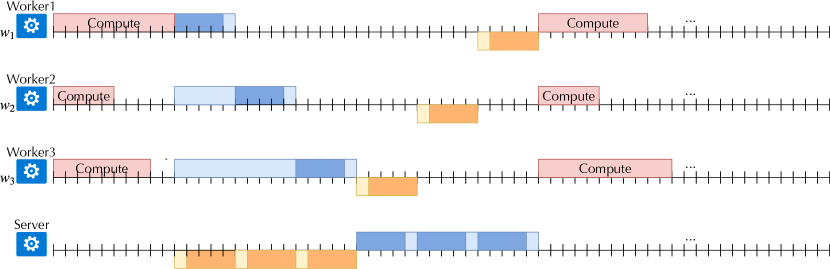
Figure 4.1: Illustration of the Impact of Asynchronous Communication (without asynchrony)

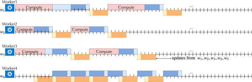
Figure 4.2: Illustration of the Impact of Asynchronous Communication (with asynchrony)

Figure 4.1 and Figure 4.2 illustrate the impact of asynchronous communication, under our simplified performance model for communication. We see that, under our current performance model, asynchronous communication can make each iteration faster — instead of waiting for all workers to finish processing, a worker can start the next iteration of computation immediately after its communication with the parameter server is finished. On the other hand, we also observe that the model used by each machine for computation might be staled. Take, for example, the last model of worker 3 $w_{3}$ in Figure 4.2 — this model misses one update from $w_{1}$ because $w_{3}$ does not wait for $w_{1}$ before it starts the next iteration of computation.

As we can see from Figure 4.2, one potential system bottleneck is the parameter server: when the server is saturated in terms of network bandwidth, adding more workers cannot make processing more data (i.e., calculating more gradients) faster without making the staleness larger. One way to accommodate this is to use multi-server parameter server architecture, in which each parameter server takes charge of one partition of the model. In this case, different partition of the model might have different staleness, which will, not surprisingly, make the theoretical analysis more engaged.

Caveats

In practice, there are other considerations that require careful attention when using asynchronous communication for distributed training. We briefly summarize these caveats and refer readers to Section 6 for further readings.

1. Bounded Staleness. If not careful, the above implementation does not necessarily provide bounded staleness — it is possible that one machine is always waiting for its communication to finish. In this case, some updates on the global replica might be using a gradient that is calculated based on a very old model, which could slow down the convergence. Some research have tried to accommodate this by enforcing bounded staleness in their implementation.

2. Straggler. When there are stragglers in the system (i.e., some machines are significantly slower than other machines), the staleness is systematic — one partition of the data is always more staled than another. In this case, staleness-aware / heterogeneous-aware algorithms could be designed to stabilize the convergence behavior.

One motivation for introducing asynchronous communication is to accommodate stragglers. There are other approaches to achieve the same objective without introducing asynchrony, however. For example, there has been research that attempts to use error correction code to make the synchronous approach more robust to stragglers. In this strategy, each worker conducts a small amount of redundant computation, such that the exact (or approximate) gradient can be recovered without waiting for the slowest $k$ machines.

4.2 Theoretical Analysis

We now analyze ASGD, a SGD variant with asynchronous communications. The updating rule of ASGD can be cast into the following form:

$${\bf x}_{t+1}={\bf x}_{t}-\gamma g_{t}({\bf x}_{\rm D(t)}),$$

where $\rm D(t)\in\{1,2,\cdots,t\}$ and ${\bf x}_{\rm D(t)}$ denote some early iterations of the model ${\bf x}_{t}$.

One important property for $g_{t}({\bf x}_{\rm D(t)})$ is

$$\mathbb{E}[g_{t}({\bf x}_{\rm D(t)})]=f^{\prime}({\bf x}_{\rm D(t)}).$$ (4.1)

To ensure the convergence rate, let us make an additional assumption about staleness:

Intuitively, to ensure convergence, the staleness cannot be overlarge. In an extreme case, if $\rm D(t)=1\;\forall t$, then the model is always updated from the true stochastic gradient in the first step, which has no hope of converging. Therefore, it is necessary to restrict the bound of $t-\rm D(t)$. In practice, the staleness parameter $t-\rm D(t)$ is proportional to the number of workers.

Next we start to show the convergence rate proof of ASGD, step by step.

$$f({\bf x}_{t+1})-f({\bf x}_{t})\leq-\gamma\langle f^{\prime}({\bf x}_{t}),g_{t}({\bf x}_{\rm D(t)})\rangle+{L\gamma^{2}\over 2}\|g_{t}({\bf x}_{\rm D(t)})\|^{2}$$

Take expectation on both sides:

$$\mathbb{E}[f({\bf x}_{t+1})]-\mathbb{E}[f({\bf x}_{t})]\leq -\gamma\mathbb{E}[\langle f^{\prime}({\bf x}_{t}),g_{t}({\bf x}_{\rm D(t)})\rangle+$$

$${L\gamma^{2}\over 2}\mathbb{E}[\|g_{t}({\bf x}_{\rm D(t)})\|^{2}]$$ (4.2)

We consider the items on the right-hand side respectively. For $\mathbb{E}[\|g_{t}({\bf x}_{\rm D(t)})\|^{2}]$, we have

$$\mathbb{E}_{\rm D(t)}[\|g_{t}({\bf x}_{\rm D(t)})\|^{2}]= \mathbb{E}_{\rm D(t)}[\|{\bf g}_{t}({\bf x}_{\rm D(t)})-f^{\prime}({\bf x}_{\rm D(t)})\|^{2}]+\|{\bf f}_{t}({\bf x}_{\rm D(t)})\|^{2}$$

$$\leq \sigma^{2}+\|{\bf f}_{t}({\bf x}_{\rm D(t)})\|^{2},$$ (4.3)

where the first equality is due to the fact (1.12), and the second is due to the bounded variance assumption, that is, Assumption 2.

For $\mathbb{E}[\langle f^{\prime}({\bf x}_{t}),g({\bf x}_{\rm D(t)})\rangle]$, we have

$$\mathbb{E}[\langle f^{\prime}({\bf x}_{t}),g({\bf x}_{\rm D(t)})\rangle]$$

$$= \mathbb{E}[\langle f^{\prime}({\bf x}_{t}),\mathbb{E}_{\rm D(t)}[g({\bf x}_{\rm D(t)})]\rangle]$$

$$= \mathbb{E}[\langle f^{\prime}({\bf x}_{t}),f^{\prime}({\bf x}_{\rm D(t)})\rangle]$$

$$= \mathbb{E}\left[{1\over 2}\|f^{\prime}({\bf x}_{t})-f^{\prime}({\bf x}_{\rm D(t)})\|^{2}-{1\over 2}\|f^{\prime}({\bf x}_{t})\|^{2}-{1\over 2}\|f^{\prime}({\bf x}_{\rm D(t)})\|^{2}\right]$$ (4.4)

The last equality uses an important property,

$$\langle{\bf a},{\bf b}\rangle={1\over 2}\|{\bf a}-{\bf b}\|^{2}-{1\over 2}\|{\bf a}\|^{2}-{1\over 2}\|{\bf b}\|^{2},$$

which can be verified by a straightforward linear algebra computation. Next we take expectation on both sides of (4.2) and plug (4.3) and (4.4) into that:

$$\mathbb{E}[f({\bf x}_{t+1})]-\mathbb{E}[f({\bf x}_{t})]$$

$$\leq -{\gamma\over 2}\mathbb{E}[\|f^{\prime}({\bf x}_{t})\|^{2}]-{\gamma\over 2}\mathbb{E}[\|f^{\prime}({\bf x}_{\rm D(t)})\|^{2}]+{\gamma\over 2}\mathbb{E}[\|f^{\prime}({\bf x}_{t})-f^{\prime}({\bf x}_{\rm D(t)})\|^{2}]$$

$$+{\gamma^{2}L\sigma^{2}\over 2}+{\gamma^{2}L\over 2}\mathbb{E}[\|f^{\prime}({\bf x}_{\rm D(t)})\|^{2}]$$

$$\leq -{\gamma\over 2}\mathbb{E}[\|f^{\prime}({\bf x}_{t})\|^{2}]+{\gamma^{2}L\sigma^{2}\over 2}-{\gamma\over 2}\left(1-{\gamma L}\right)\mathbb{E}[\|f^{\prime}({\bf x}_{\rm D(t)})\|^{2}]$$

$$+{\gamma\over 2}\mathbb{E}[\|f^{\prime}({\bf x}_{t})-f^{\prime}({\bf x}_{\rm D(t)})\|^{2}]$$

$$\leq -{\gamma\over 2}\mathbb{E}[\|f^{\prime}({\bf x}_{t})\|^{2}]+{\gamma^{2}L\sigma^{2}\over 2}+{\gamma\over 2}\mathbb{E}[\|f^{\prime}({\bf x}_{t})-f^{\prime}({\bf x}_{\rm D(t)})\|^{2}],$$ (4.5)

where the last inequality is obtained by choosing a sufficiently small learning rate $\gamma$ satisfying

$$1\geq\gamma L.$$ (4.6)

We have seen the first two terms on the right-hand side of (4.5) (if ignoring the constant parts) in the proof to SGD. We can roughly treat this term as $\mathbb{E}\|f^{\prime}({\bf x}_{t})\|^{2}$ plus some perturbation, depending on the staleness $\tau$. The major term we need to treat very seriously is the last term $\mathbb{E}[\|f^{\prime}({\bf x}_{t})-f^{\prime}({\bf x}_{\rm D(t)})\|^{2}]$, whose upper bound is given by the following lemma. It basically shows that this item is bounded by a higher order of $\gamma$: $O(\gamma^{3})$.

Proof 4.2.2.

We start by bounding the difference between $f^{\prime}({\bf x}_{t})$ and $f^{\prime}({\bf x}_{\rm D(t)})$

$$\mathbb{E}[\|f^{\prime}({\bf x}_{t})-f^{\prime}({\bf x}_{\rm D(t)})\|^{2}]$$

$$\leq L^{2}\mathbb{E}[\|{\bf x}_{t}-{\bf x}_{t_{\tau_{t}}}\|^{2}]\quad(\text{Due to Assumption\leavevmode\nobreak\ \ref{ass:gd}})$$

$$= \gamma^{2}L^{2}\mathbb{E}\left[\left\|\sum_{s=\rm D(t)}^{t-1}g_{s}({\bf x}_{\rm D(s)})\right\|^{2}\right].$$

$$= \gamma^{2}L^{2}\mathbb{E}\left[\left\|\sum_{s=\rm D(t)}^{t-1}g_{s}({\bf x}_{\rm D(s)})-\sum_{s=\rm D(t)}^{t-1}f^{\prime}_{s}({\bf x}_{\rm D(s)})+\sum_{s=\rm D(t)}^{t-1}f^{\prime}_{s}({\bf x}_{\rm D(s)})\right\|^{2}\right]$$

$$\leq 2\gamma^{2}L^{2}\mathbb{E}\left[\left\|\sum_{s=\rm D(t)}^{t-1}\underbrace{\left(g_{s}({\bf x}_{\rm D(s)})-f^{\prime}_{s}({\bf x}_{\rm D(s)})\right)}_{=:\xi_{s-\rm D(t)}}\right\|^{2}\right]$$

$$+2\gamma^{2}L^{2}\mathbb{E}\left[\left\|\sum_{s=\rm D(t)}^{t-1}f^{\prime}_{s}({\bf x}_{\rm D(s)})\right\|^{2}\right],$$ (4.7)

where the last inequality uses a variant of triangle inequality $\|{\bf a}+{\bf b}\|^{2}\leq 2\|{\bf a}\|^{2}+2\|{\bf b}\|^{2}$. Note that the sequence of $\{\xi_{0},\xi_{1},\cdots,\xi_{\tau_{t}-\rm D(t)-1}\}$ is a martingale sequence with

$$\xi_{l}:=g_{s+l}({\bf x}_{\rm D(s+l)})-f^{\prime}_{s+l}({\bf x}_{\rm D(s+l)}).$$

A martingale sequence satisfies that

$$\mathbb{E}(\xi_{l+1}\leavevmode\nobreak\ |\leavevmode\nobreak\ \xi_{0},\xi_{1},\cdots,\xi_{l})=0.$$

Therefore, it is easy to verify that

$$\mathbb{E}\left[\left\|\sum_{l=0}^{t-1-\rm D(t)}\xi_{l}\right\|^{2}\right]= \mathbb{E}\left[\left\|\sum_{l=0}^{t-2-\rm D(t)}\xi_{l}\right\|^{2}\right]+\mathbb{E}\left[\left\|\xi_{t-1}\right\|^{2}\right]$$

$$= \sum_{l=0}^{t-1-\rm D(t)}\mathbb{E}\left[\|\xi_{l}\|^{2}\right].$$

In other words, we have

$$\mathbb{E}\left[\left\|\sum_{s=\rm D(t)}^{t-1}\left(g_{s}({\bf x}_{\rm D(s)})-f^{\prime}_{s}({\bf x}_{\rm D(s)})\right)\right\|^{2}\right]=\sum_{l=0}^{t-1-\rm D(t)}\mathbb{E}\left[\|\xi_{l}\|^{2}\right]\leq\tau\sigma^{2}.$$

Applying this property to (4.7) yields

$$\mathbb{E}[\|f^{\prime}({\bf x}_{t})-f^{\prime}({\bf x}_{\rm D(t)})\|^{2}]$$

$$\leq 2\gamma^{2}L^{2}\tau\sigma^{2}+2\gamma^{2}L^{2}\mathbb{E}\left[\left\|\sum_{s=\rm D(t)}^{t-1}f^{\prime}_{s}({\bf x}_{\rm D(s)})\right\|^{2}\right]$$

$$\leq 2\gamma^{2}L^{2}\tau\sigma^{2}+2\gamma^{2}L^{2}\tau\sum_{s=\rm D(t)}^{t-1}\mathbb{E}\left[\left\|f^{\prime}_{s}({\bf x}_{\rm D(s)})\right\|^{2}\right],$$

where the last inequality uses Assumption 5 the following property: for any vectors ${\bf a}_{1},{\bf a}_{2},\cdots,{\bf a}_{n}$, we have

$$\left\|\sum_{i=1}^{n}{\bf a}_{i}\right\|^{2}\leq n\sum_{i=1}^{n}\|{\bf a}_{i}\|^{2}.$$

This completes the proof.

We choose the learning rate to be sufficiently small. In particular, let

$$\gamma L\tau\leq 1/2.$$ (4.8)

Using the following short notations:

$$a_{t}:= \mathbb{E}[\|f^{\prime}({\bf x}_{t})\|^{2}]$$

$$b_{t}:= \mathbb{E}[f({\bf x}_{t})],$$

and apply Lemma 5.2.7 to (4.5):

$$b_{t+1}-b_{t}\leq -{\gamma\over 2}a_{t}+{\gamma^{2}L\over 2}\left(1+2\gamma L\tau\right)\sigma^{2}+{\gamma^{3}L^{2}\tau}\sum_{s=\rm D(t)}^{t-1}a_{s}$$

$$\leq -{\gamma\over 2}a_{t}+{\gamma^{2}L\over 2}\left(1+2\gamma L\tau\right)\sigma^{2}+{\gamma^{3}L^{2}\tau}\sum_{s=\rm D(t)}^{t-1}a_{s}$$

$$\leq -{\gamma\over 2}a_{t}+{\gamma^{2}L}\sigma^{2}+{\gamma\over 4\tau}\sum_{s=\rm D(t)}^{t-1}a_{s}.$$ (4.9)

Next we take sum of (4.9) over $t$ from $t=1$ to $t=T$

$$b_{T+1}-b_{1}\leq -{\gamma\over 2}\sum_{t=1}^{T}a_{t}+\gamma^{2}LT\sigma^{2}+{\gamma\over 4\tau}\sum_{t=1}^{T}\sum_{s=\rm D(t)}^{t-1}a_{s}$$

$$\leq -{\gamma\over 2}\sum_{t=1}^{T}a_{t}+\gamma^{2}LT\sigma^{2}+{\gamma\over 4}\sum_{t=1}^{T}a_{t}$$

$$= -{\gamma\over 4}\sum_{t=1}^{T}a_{t}+\gamma^{2}LT\sigma^{2}.$$

Therefore, we have the following convergence rate:

$${1\over T}\sum_{t=1}^{T}a_{t}\leq{4(b_{1}-b_{T+1})\over\gamma T}+{4\gamma L\sigma^{2}}.$$

If we treat $f({\bf x}_{1})-f^{\star}$ to be constant, then we have

$${1\over T}\sum_{t=1}^{T}\mathbb{E}\left\|f^{\prime}({\bf x}_{t})\right\|^{2}\lesssim \frac{f({\bf x}_{1})-\mathbb{E}\left[f({\bf x}_{T+1})\right]}{\gamma T}+\gamma L\sigma^{2}$$

$$\lesssim \frac{f({\bf x}_{1})-f^{\star}}{\gamma T}+\gamma L\sigma^{2}$$

$$\lesssim \frac{1}{\gamma T}+\gamma L\sigma^{2}.$$

We choose the learning rate $\gamma$ to be

$$\gamma=\frac{1}{L(\tau+1)+\sqrt{TL}\sigma}$$ (4.10)

to satisfy the requirements of $\gamma$ in (4.6) and (4.8), which leads to

$${1\over\gamma T}\leq {L(\tau+1)\over T}+{\sqrt{L}\sigma\over\sqrt{T}}$$

$$\gamma L\sigma^{2}\leq {\sqrt{L}\sigma\over\sqrt{T}}.$$

Therefore, we can summarize the convergence rate of ASGD in the following theorem.

We highlight the following observations from this convergence analysis:

• (Consistency to SGD) If there is only one worker, then $\tau=0$ and the ASGD algorithm reduces the SGD algorithm. We can see that the convergence rate in Theorem 4.2.3 is consistent with SGD.

• (Linear speedup) The additional term in the rate is the last term, as compared to SGD. It is caused by the asynchronous parallelism. Recall that $\tau$ is proportional to the total number of workers. If $\tau$ satisfies $\tau\leq{\sqrt{T}\sigma\over\sqrt{L}}$, then the convergence efficiency would not be affected by using asynchronous updating. As a result, linear speedup can be achieved. Here, the linear speedup is in the sense that the average computational complexity per worker is asymptotically the computational complexity using one single worker divided by $N$ – the total number of workers.

Chapter 5 System Relaxation 3: Decentralized Communication

Lossy communication compression is designed to alleviate system bottlenecks caused by network bandwidth. Another type of network bottleneck is caused by latency. In that case, when there are $N$ workers, both the AllReduce and the multi-server parameter server have an $O(N)$ dependency on the network latency. The fundamental reason for this is that all these approaches insist that the information on each worker be propagated to all other workers in a single round of communication.

There are multiple standard ways to get rid of the latency bottleneck, e.g., using a textbook reduction tree. In this Section, we describe an alternative approach to improving the latency overhead. We call this method decentralized communication. Specifically, we form a logical ring among $N$ workers (all workers are still connected via the same “logical switch”). At every single iteration, a worker sends one message to the neighbor on its immediate left and one message to the neighbor on its immediate right. With this method, the latency overhead becomes $O(1)$. On the downside, however, the information on a single worker only reaches its two adjacent neighbors in one round of communication.

5.1 System Implementation

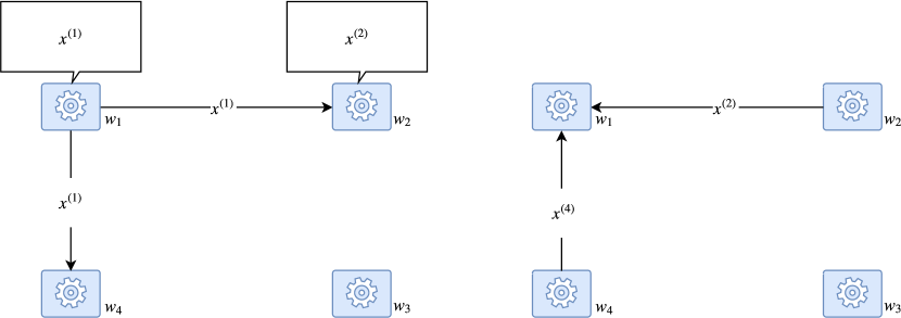
Figure 5.1: Illustration of Decentralized Communication Pattern on the first worker $w_{1}$ (other workers are similar). Each worker holds a local model replica and only sends this model to the neighbors on its immediate right and left.

To implement this system relaxation, we rely on a communication pattern like that of the model aggregation approach for implementing distributed SGD instead of exchanging gradients as we did in the previous Sectionon system exchange models. Specifically,

1. At step $t$, each worker $w_{n}$ holds a model replica ${\bf x}_{t}^{(n)}$. The system first calculates the stochastic gradient using its local replica $f^{\prime}(x^{(n)})$ and then updates its local model using this standard SGD rule:

   $${\bf x}_{t+1/2}^{(n)}={\bf x}_{t}^{(n)}-\gamma f^{\prime}({\bf x}^{(n)}).$$

2. Each worker $w_{n}$ sends its locally updated model $x_{t+1/2}^{(n)}$ to the neighbor on its immediate right, $w_{(n+1)\mod N}$, and to the neighbor on its immediate left, $w_{(n-1)\mod N}$. Symmetrically, the worker will also receive models from the neighbor on its immediate right, $w_{(n+1)\mod N}$, and from the neighbor on its immediate left, $w_{(n-1)\mod N}$. Upon receiving the neighbors’ models, the worker updates its local model as the average between its local model and its neighbors’ models:

   $${\bf x}_{t+1}^{(n)}=\frac{1}{3}\left({\bf x}_{t+1/2}^{(n)}+{\bf x}_{t+1/2}^{((n+1)\mod N)}+{\bf x}_{t+1/2}^{((n-1)\mod N)}\right).$$

Impact of Decentralized Communication

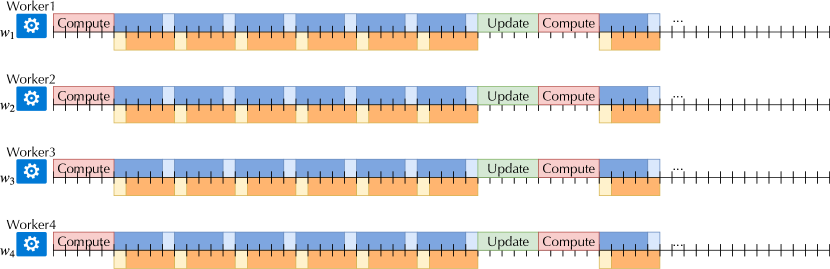
Figure 5.2: Illustration of the Impact of Decentralized Communication (without decentralization)

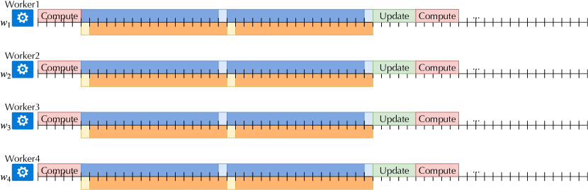
Figure 5.3: Illustration of the Impact of Decentralized Communication (with decentralization)

The communication cost for one round of communication in the decentralized setting is

$$2t_{\text{latency}}+2t_{\text{transfer}}.$$

Recall that the communication cost of the multi-server parameter server or the AllReduce is

$$2(N-1)t_{\text{latency}}+2\frac{N-1}{N}t_{\text{transfer}}.$$

With our method, we see a clear improvement with the decentralized communication in terms of communication latency. When the underlying network has a high latency, the decentralized strategy can be significantly faster.

Figure 5.2 and Figure 5.3 illustrate the communication patterns. Interestingly, in this specific example, the decentralized approach communication might seem to take longer. This happens because, when there are $n$ workers, each worker only needs to send $\frac{N-1}{N}$ of its model in the centralized case instead of the full model. In the decentralized case, workers need to exchange their full models. As a result, the transfer time of the decentralized approach might be slightly higher. However, as illustrated in Figure 5.3, the decentralized approach has an advantage in terms of latency, and this improvement will be more significant when there are more workers and the underlying network has a higher latency.

More generally, one can extend the above example beyond a simple ring topology. We consider this below in the theoretical analysis.

5.2 Theoretical Analysis

We analyze DSGD, a SGD variant with decentralized communication. Let us consider the same objective as (3.9). For convenience of reference, we repeat it again here

$$\min_{{\bf x}}:\quad\left\{f({{\bf x}}):={1\over N}\sum_{n=1}^{N}f_{n}({\bf x})\right\}$$ (5.1)

where $f_{n}({{\bf x}}):=\mathbb{E}_{\xi\sim\mathcal{D}_{n}}F_{n}({\bf x};\xi)$ and $\mathcal{D}_{n}$ denotes the distribution of local data at node $n$. We do not assume that all nodes can access the whole dataset.

Based on the algorithm description in the previous section, the DSGD algorithm’s updating rule can be cast in the following form:

$${\bf X}_{t+1}=\left({\bf X}_{t}-\gamma{\bf G}\left({\bf X}_{t};\{\xi_{t}^{(n)}\}_{n=1}^{N}\right)\right)W.$$ (5.2)

Here we use the following notations:

$${\bf X}_{t}:= \left[{\bf x}^{(1)}_{t},{\bf x}^{(2)}_{t},\cdots,{\bf x}^{(N)}_{t}\right]$$

$${\bf G}\left({\bf X}_{t};\{\xi_{t}^{(n)}\}_{n=1}^{N}\right):= \left[F^{\prime}_{1}\left({\bf x}^{(1)}_{t};\xi_{t}^{(1)}\right),\cdots,F^{\prime}_{N}\left({\bf x}^{(N)}_{t};\xi_{t}^{(N)}\right)\right]$$

where ${\bf x}_{t}^{(n)}$ denotes the local model on node $n$ at time $t$. We also use ${\bf G}_{t}$ to denote ${\bf G}\left({\bf X}_{t};\{\xi_{t}^{(n)}\}_{n=1}^{N}\right)$ for short. $W\in{\bf R}^{N\times N}$ is called the confusion matrix.

5.2.1 Assumptions

To show the convergence rate of DSGD, we need to make a few important assumptions about the objective function:

The first assumption on the smoothness and the Lipschitz gradient is essentially the same as Assumption 1. The second assumption is essentially that all local stochastic gradients are locally unbiased. The bounded inner variance assumption assumes that all local stochastic gradients have a bounded local variance that is similar to Assumption 2. The last assumption is that the total gradient difference among workers is bounded. If all workers access the same dataset, then $\varsigma=0$.

We next make the necessary assumptions for the confusion matrix $W$:

$W^{\top}{\bf 1}=1$ is to ensure that the weighted sum is $1$ when take the average of models, and the symmetry ensures that all eigenvalues of $W$ are real numbers. The spectral gap $1-\rho$ roughly measures how fast the information can be spread over the network. The smaller $\rho$ is, the faster the communication is. Note that since $W$ is doubly stochastic, the largest eigenvalue is always $1$. Let us look at a few examples to get some sense of the value of $\rho$:

$$W_{1}= {{\bf 1}{\bf 1}^{\top}\over N}, \rho=0$$

$$W_{2}= \left[\begin{matrix}{1\over 3}&{1\over 3}&0&\cdots&0&{1\over 3}\\ {1\over 3}&{1\over 3}&{1\over 3}&0&\cdots&0\\ 0&{1\over 3}&{1\over 3}&{1\over 3}&\cdots&0\\ \vdots&\vdots&\vdots&\vdots&\vdots&\vdots\\ 0&\cdots&0&{1\over 3}&{1\over 3}&{1\over 3}\\ {1\over 3}&0&\cdots&0&{1\over 3}&{1\over 3}\end{matrix}\right] \rho\approx 1-{16\pi^{2}\over 3N^{2}}$$

$$W_{3}= \left[\begin{matrix}\text{any doubly stochastic matrix}&{\bf 0}\\ {\bf 0}^{\top}&1\end{matrix}\right] \rho=1.$$

$W_{1}$ (with $\rho=1$) corresponds to the fully connected network, which is the fastest network for spreading information; $W_{2}$ (with a $\rho$ value close to but smaller than $1$) corresponds to the ring network; $W_{3}$ (with $\rho=1$) corresponds to a disconnected network, which does work for DSGD.

The last assumption we make is about the initial local models, which we assume to be identical. This assumption is not necessary (we can obtain a similar result without it) but can simplify notations and derivations in the proof.

5.2.2 Convergence rate

The theoretical analysis for DSGD is relatively complicated. Readers can jump directly to Theorem 5.2.11 if they are not interested in the convergence proof.

To simplify the notations used in our proof, let us define some new notations for convenience. Denote by

$$f^{\prime}\left({\bf X}_{t}\right):= \left[f^{\prime}_{1}\left({\bf x}^{(1)}_{t}\right),f^{\prime}_{2}\left({\bf x}^{(2)}_{t}\right),\cdots,f^{\prime}_{N}\left({\bf x}^{(N)}_{t}\right)\right]$$

$$\bar{f}^{\prime}({\bf X}_{t}):= f^{\prime}({\bf X}_{t}){{\bf 1}\over N},$$

$$\bar{{\bf x}}_{t}:= {\bf X}_{t}{{\bf 1}\over N},$$

$$\bar{{\bf X}}_{t}:= {\bf X}_{t}{{\bf 11}^{\top}\over N},$$

$$\bar{{\bf g}}_{t}:= {\bf G}_{t}{{\bf 1}\over N}.$$

Then it is not hard to see that

$$\mathbb{E}\left[{\bf G}\left({\bf X}_{t};\{\xi_{t}^{(n)}\}_{n=1}^{N}\right)\right]=f^{\prime}\left({\bf X}_{t}\right).$$ (5.3)

We next show some preliminary results that illustrate our final proof:

Proof 5.2.2.

We first bound the difference between $\bar{f}^{\prime}({\bf X}_{t})$ and $f^{\prime}(\bar{{\bf x}}_{t})$:

$$\left\|\bar{f^{\prime}}({\bf X}_{t})-f^{\prime}(\bar{{\bf x}}_{t})\right\|^{2}= \left\|{1\over N}\sum_{n=1}^{N}f^{\prime}_{n}({\bf x}^{(n)}_{t})-{1\over N}\sum_{n=1}^{N}f^{\prime}_{n}\left(\bar{{\bf x}}_{t}\right)\right\|^{2}$$

$$= {1\over N^{2}}\left\|\sum_{n=1}^{N}f^{\prime}_{n}({\bf x}^{(n)}_{t})-\sum_{n=1}^{N}f^{\prime}_{n}\left(\bar{{\bf x}}_{t}\right)\right\|^{2}$$

$$\leq {1\over N}\sum_{n=1}^{N}\left\|f^{\prime}_{n}({\bf x}^{(n)}_{t})-f^{\prime}_{n}\left(\bar{{\bf x}}_{t}\right)\right\|^{2}$$

$$\leq {L^{2}\over N}\sum_{n=1}^{N}\|{\bf x}_{t}^{(n)}-\bar{{\bf x}}_{t}\|^{2}$$

$$= {L^{2}\over N}\|{\bf X}_{t}-\bar{{\bf X}}_{t}\|^{2}_{F}$$

where the first inequality uses the property

$$\left\|\sum_{n=1}^{N}{\bf z}^{(n)}\right\|^{2}\leq N\sum_{n=1}^{N}\left\|{\bf z}^{(n)}\right\|^{2}.$$

Next, we prove the second inequality by using Assumption 6 (smoothness):

$${1\over 2}\left\|f^{\prime}({\bf X}_{t})-f^{\prime}(\bar{{\bf x}}_{t}){\bf 1}^{\top}\right\|^{2}_{F}$$

$$= {1\over 2}\left\|f^{\prime}({\bf X}_{t})-f^{\prime}(\bar{{\bf X}}_{t})+f^{\prime}(\bar{{\bf X}}_{t})-f^{\prime}(\bar{{\bf x}}_{t}){\bf 1}^{\top}\right\|^{2}_{F}$$

$$\leq \left\|f^{\prime}({\bf X}_{t})-f^{\prime}(\bar{{\bf X}}_{t})\right\|^{2}_{F}+\left\|f^{\prime}(\bar{{\bf X}}_{t})-f^{\prime}(\bar{{\bf x}}_{t}){\bf 1}^{\top}\right\|^{2}_{F}$$

$$\leq L^{2}\|{\bf X}_{t}-\bar{{\bf X}}_{t}\|^{2}_{F}+\left\|{f}^{\prime}(\bar{{\bf X}}_{t})-f^{\prime}(\bar{{\bf x}}_{t}){\bf 1}^{\top}\right\|^{2}_{F}$$

$$= L^{2}\|{\bf X}_{t}-\bar{{\bf X}}_{t}\|^{2}_{F}+\sum_{n=1}^{N}\left\|f^{\prime}_{n}(\bar{{\bf x}}_{t})-f^{\prime}(\bar{{\bf x}}_{t})\right\|^{2}$$

$$\leq L^{2}\|{\bf X}_{t}-\bar{{\bf X}}_{t}\|^{2}_{F}+N\varsigma^{2}.$$

Next, we prove the last inequality:

$$\mathbb{E}\left[\left\|{\bf G}_{t}\right\|^{2}\right]= \left\|\mathbb{E}\left[{\bf G}_{t}\right]\right\|^{2}_{F}+\mathbb{E}\left\|{\bf G}_{t}-\mathbb{E}\left[{\bf G}_{t}\right]\right\|^{2}_{F}$$

$$\leq \left\|f^{\prime}({\bf X}_{t})\right\|^{2}_{F}+N\sigma^{2}$$

$$\leq 2\left\|f^{\prime}({\bf X}_{t})-f^{\prime}(\bar{{\bf x}}_{t}){\bf 1}^{\top}\right\|^{2}_{F}+2\left\|f^{\prime}(\bar{{\bf x}}_{t}){\bf 1}^{\top}\right\|^{2}_{F}+N\sigma^{2}$$

$$= 2\left\|f^{\prime}({\bf X}_{t})-f^{\prime}(\bar{{\bf x}}_{t}){\bf 1}^{\top}\right\|^{2}_{F}+2N\left\|f^{\prime}(\bar{{\bf x}}_{t})\right\|^{2}+N\sigma^{2}.$$

Next, we prove a useful inequality:

Proof 5.2.4.

Consider the left-hand side:

$$\sum_{t=1}^{k}a_{t}^{2}= \sum_{t=1}^{k}\sum_{s=1}^{t}\rho^{t-s}b_{s}\sum_{r=1}^{t}\rho^{t-r}b_{r}$$

$$= \sum_{t=1}^{k}\sum_{s=1}^{t}\sum_{r=1}^{t}\rho^{2t-s-r}b_{s}b_{r}$$

$$\leq \sum_{t=1}^{k}\sum_{s=1}^{t}\sum_{r=1}^{t}\rho^{2t-s-r}{b_{s}^{2}+b_{r}^{2}\over 2}$$

$$= \sum_{t=1}^{k}\sum_{s=1}^{t}\sum_{r=1}^{t}\rho^{2t-s-r}b_{s}^{2}$$

$$\leq {1\over 1-\rho}\sum_{t=1}^{k}\sum_{s=1}^{t}\rho^{t-s}b_{s}^{2}$$

$$\leq {1\over(1-\rho)^{2}}\sum_{s=1}^{k}b_{s}^{2}.$$

This completes the proof.

Given these preliminary results, we can show the first inequality for the upper bound of the total model variation, that is, the distance between the local models ${\bf X}_{t}$ and the average model $\bar{{\bf X}}_{t}$. In attempting to understand the decentralized algorithm, the first question people may ask is whether all local models will achieve consensus eventually as the centralized counterpart always satisfies the consensus over all iterations. Lemma 5.2.7 essentially shows that DSGD can ensure that all ${\bf x}_{t}^{(n)}$s converge to $\bar{{\bf x}}_{t}$. This happens because the total variation $\sum_{t=1}^{T}\mathbb{E}\left[\|\bar{{\bf X}}_{t}-{\bf X}_{t}\|^{2}_{F}\right]$ is roughly bounded by $O(\gamma^{2}T)$. Based on our experiences of analyzing stochastic algorithms, we know that the learning rate is usually proportional to $1/\sqrt{T}$. Therefore, the total variation is bounded by a constant, which indicates that all ${\bf x}_{t}^{(n)}$ converges to $\bar{{\bf x}}_{t}$.

Proof 5.2.6.

From the updating rule, we obtain the following closed form for ${\bf X}_{t}$ and $\bar{{\bf X}}_{t}$:

$${\bf X}_{t}= \gamma\sum_{s=1}^{t-1}{\bf G}_{s}W^{t-s}$$

$$\bar{{\bf X}}_{t}= {\bf X}_{t}{{\bf 11}^{\top}\over N}$$

Next, we bound the difference between $\bar{{\bf X}}_{t}$ and ${\bf X}_{t}$ as follows:

$${1\over\gamma}\left\|{\bf X}_{t}-\bar{{\bf X}}_{t}\right\|_{F}$$

$$= {1\over\gamma}\left\|{\bf X}_{t}\left(I-{{\bf 11}^{\top}\over N}\right)\right\|_{F}$$

$$= \left\|\sum_{s=1}^{t-1}{\bf G}_{s}W^{t-s}\left(I-{{\bf 11}^{\top}\over N}\right)\right\|_{F}$$

$$= \left\|\sum_{s=1}^{t-1}{\bf G}_{s}\left(W^{t-s}-{{\bf 11}^{\top}\over N}\right)\right\|_{F}\quad\left(\text{due to}\leavevmode\nobreak\ W{\bf 1}={\bf 1}\right)$$

$$\leq \sum_{s=1}^{t-1}\left\|{\bf G}_{s}\left(W^{t-s}-{{\bf 11}^{\top}\over N}\right)\right\|_{F}\quad\left(\text{due to the triangle inequality}\right)$$

$$\leq \sum_{s=1}^{t-1}\left\|{\bf G}_{s}\right\|_{F}\left\|\left(W^{t-s}-{{\bf 11}^{\top}\over N}\right)\right\|\quad\left(\text{due to $\|AB\|_{F}\leq\|A\|_{F}\|B\|$}\right)$$

$$\leq \sum_{s=1}^{t-1}\rho^{t-s}\left\|{\bf G}_{s}\right\|_{F}.$$

Taking the square and the sum over $t$, the equation above becomes

$$\sum_{t=1}^{T}\frac{1}{\gamma^{2}}\left\|{\bf X}_{t}-\bar{{\bf X}}_{t}\right\|_{F}^{2}$$

$$\leq \sum_{t=1}^{T}\rho^{2}\left(\sum_{s=1}^{t-1}\rho^{t-s-1}\left\|{\bf G}_{s}\right\|_{F}\right)^{2}$$

$$\leq \frac{\rho^{2}}{(1-\rho)^{2}}\sum_{t=1}^{T}\left\|{\bf G}_{t}\right\|_{F}^{2}\quad\text{(due to Lemma\leavevmode\nobreak\ \ref{lem:dsgd:seq})}.$$

This completes the proof.

Proof 5.2.8.

Applying Lemma 5.2.1 to Lemma 5.2.5 gives

$$\frac{(1-\rho)^{2}}{\gamma^{2}\rho^{2}}\mathbb{E}\left[\|\bar{{\bf X}}_{t}-{\bf X}_{t}\|^{2}_{F}\right]\leq 2N\mathbb{E}\left[\|f^{\prime}(\bar{{\bf x}}_{t})\|^{2}\right]+$$

$$4L^{2}\mathbb{E}\left\|\bar{{\bf X}}_{t}-{{\bf X}}_{t}\right\|^{2}_{F}+4N\varsigma^{2}+N\sigma^{2}.$$

Given the restriction on the learning rate $\gamma$, we have $4L^{2}\leq(1-\rho)^{2}/(2\gamma^{2}\rho^{2})$ and thus obtain

$$\frac{(1-\rho)^{2}}{\gamma^{2}\rho^{2}}\mathbb{E}\left[\|\bar{{\bf X}}_{t}-{\bf X}_{t}\|^{2}_{F}\right]\leq 2N\mathbb{E}\left[\|f^{\prime}(\bar{{\bf x}}_{t})\|^{2}\right]+$$

$$+8N(\varsigma^{2}+\sigma^{2}),$$

which completes the proof.

Proof 5.2.10.

Let us start with a basic property:

$$\mathbb{E}[\bar{{\bf g}}_{t}]={1\over N}\sum_{n=1}^{N}f^{\prime}_{n}({\bf x}^{(n)}_{t})=:\bar{f^{\prime}}({\bf X}_{t})$$ (5.8)

We consider the improvement of $\mathbb{E}\left[f(\bar{{\bf x}}_{t+1})\right]$ over $\mathbb{E}\left[f(\bar{{\bf x}}_{t})\right]$ in the following:

$$\mathbb{E}\left[f(\bar{{\bf x}}_{t+1})\right]-\mathbb{E}\left[f(\bar{{\bf x}}_{t})\right]$$

$$\leq \mathbb{E}\langle f^{\prime}(\bar{{\bf x}}_{t}),-\gamma\bar{{\bf g}}_{t}\rangle+{L\gamma^{2}\over 2}\mathbb{E}\left[\|\bar{{\bf g}}_{t}\|^{2}\right]$$

$$= -\gamma\mathbb{E}\langle f^{\prime}(\bar{{\bf x}}_{t}),\bar{f^{\prime}}({\bf X}_{t})\rangle+{L\gamma^{2}\over 2}\mathbb{E}\left[\|\bar{{\bf g}_{t}}\|^{2}\right]$$

$$= -{\gamma\over 2}\mathbb{E}\|f^{\prime}(\bar{{\bf x}}_{t})\|^{2}-{\gamma\over 2}\mathbb{E}\|\bar{f^{\prime}}({{\bf X}}_{t})\|^{2}+{\gamma\over 2}\mathbb{E}\|\bar{f^{\prime}}({\bf X}_{t})-f^{\prime}(\bar{{\bf x}}_{t})\|^{2}+$$

$$+{L\gamma^{2}\over 2}\mathbb{E}\left[\|\bar{{\bf g}}_{t}\|^{2}\right].$$ (5.9)

We look at the last term first in the above inequality:

$$\mathbb{E}\left[\|\bar{{\bf g}}_{t}\|^{2}\right]= \left\|\mathbb{E}\left[\bar{{\bf g}}_{t}\right]\right\|^{2}+\mathbb{E}\left[\left\|\bar{{\bf g}}_{t}-\mathbb{E}\left[\bar{{\bf g}}_{t}\right]\right\|^{2}\right]$$

$$\leq \|\bar{f^{\prime}}({\bf X}_{t})\|^{2}+{\sigma^{2}\over N}$$ (5.10)

where the inequality uses the property of $\bar{{\bf g}}_{t}$ in (5.8) and the property for any i.i.d. random variables $z^{(1)},\cdots,z^{(n)}$

$${\bf Var}\left({1\over N}\sum_{n=1}^{N}z^{(n)}\right)={1\over N}{\bf Var}(z^{(n)}),$$

together with the boundedness in Assumption 6.

Plugging (5.10) and (5.4) into (5.9) yields

$$\mathbb{E}\left[f(\bar{{\bf x}}_{t+1})\right]-\mathbb{E}\left[f(\bar{{\bf x}}_{t})\right]$$

$$\leq -{\gamma\over 2}\mathbb{E}\|f^{\prime}(\bar{{\bf x}}_{t})\|^{2}-\left({\gamma\over 2}-{L\gamma^{2}\over 2}\right)\mathbb{E}\|\bar{f^{\prime}}({{\bf X}}_{t})\|^{2}+$$

$${L^{2}\gamma\over 2N}\mathbb{E}\left\|{{\bf X}}_{t}-\bar{{\bf X}}_{t}\right\|^{2}_{F}+{L\gamma^{2}\sigma^{2}\over 2N}$$

$$\leq -{\gamma\over 2}\mathbb{E}\|f^{\prime}(\bar{{\bf x}}_{t})\|^{2}+{L^{2}\gamma\over 2N}\mathbb{E}\left\|{{\bf X}}_{t}-\bar{{\bf X}}_{t}\right\|^{2}_{F}+{L\gamma^{2}\sigma^{2}\over 2N}.$$

This completes the proof.

Now we are ready to show the main result.

Proof 5.2.12.

Taking the summarization over $t$ from $t=1$ to $t=T$ for Lemma 5.2.9 yields

$${1\over T}\sum_{t=1}^{T}\mathbb{E}\left\|f^{\prime}(\bar{{\bf x}}_{t})\right\|^{2}$$

$$\leq {2\over T\gamma}\left(f(\bar{{\bf x}}_{0})-f^{\star}\right)+\frac{L\sigma^{2}\gamma}{N}+{L^{2}\over NT}\sum_{t=1}^{T}\left\|\bar{{\bf X}}_{t}-{\bf X}_{t}\right\|^{2}_{F}$$

$$\leq {2\over T\gamma}\left(f(\bar{{\bf x}}_{0})-f^{\star}\right)+\frac{L\sigma^{2}\gamma}{N}+$$

$$\frac{8L^{2}\varsigma^{2}\gamma^{2}}{(1-\rho)^{2}}+\frac{8L^{2}\sigma^{2}\gamma^{2}\rho^{2}}{(1-\rho)^{2}}+\frac{2L^{2}\gamma^{2}\rho^{2}}{(1-\rho)^{2}T}\sum_{t=1}^{T}\mathbb{E}\|f^{\prime}(\bar{{\bf x}}_{t})\|^{2}.$$

From the restriction on the learning rate, we have

$$\frac{8L^{2}\sigma^{2}\gamma^{2}\rho^{2}}{(1-\rho)^{2}}\leq\frac{L\sigma^{2}\gamma}{N}$$

and

$${2L^{2}\gamma^{2}\rho^{2}\over(1-\rho)^{2}}\leq{1\over 2}.$$

It follows that

$${1\over 2T}\sum_{t=1}^{T}\mathbb{E}\left\|f^{\prime}(\bar{{\bf x}}_{t})\right\|^{2}$$

$$\leq {2\over T\gamma}\left(f(\bar{{\bf x}}_{0})-f^{\star}\right)+\frac{L\sigma^{2}\gamma}{N}+{L^{2}\over NT}\sum_{t=1}^{T}\left\|\bar{{\bf X}}_{t}-{\bf X}_{t}\right\|^{2}_{F}$$

$$\leq {2\over T\gamma}\left(f(\bar{{\bf x}}_{0})-f^{\star}\right)+\frac{2L\sigma^{2}\gamma}{N}+\frac{8L^{2}\varsigma^{2}\gamma^{2}\rho^{2}}{(1-\rho)^{2}}$$

For simplicity, we treat $f(\bar{{\bf x}}_{0})-f^{\star}$ and $L$ as constants and obtain the following simplified inequality:

$${1\over T}\sum_{t=1}^{T}\mathbb{E}\left\|f^{\prime}(\bar{{\bf x}}_{t})\right\|^{2}\lesssim {1\over T\gamma}+\frac{\sigma^{2}\gamma}{N}+\frac{\varsigma^{2}\gamma^{2}\rho^{2}}{(1-\rho)^{2}}.$$

Due to the form of the learning rate in (5.11), we have

$$\frac{1}{T\gamma}\leq {1\over T}+{\sigma\over\sqrt{NT}}+{\varsigma^{2/3}\over T^{2/3}(1-\rho)^{2/3}}$$

$$\frac{\sigma^{2}\gamma}{N}\leq {\sigma\over\sqrt{NT}}$$

$$\frac{\varsigma^{2}\gamma^{2}\rho^{2}}{1-\rho}\leq {\varsigma^{2/3}\rho^{2/3}\over T^{2/3}(1-\rho)^{2/3}},$$

which completes the proof.

We highlight the following observations from this convergence analysis:

• (Consistency to mb-SGD) If we use the fully connected network, then $\rho=0$ and the DSGD algorithm reduces the (centralized) mb-SGD algorithm. We can see that the convergence rate in Theorem (5.2.11) is consistent with mb-SGD, since the last term becomes zero.

• (Linear speedup) The additional term in the rate is the the last term, comparing to mb-SGD. It is caused by using decentralized updating. As long as $T$ is sufficiently large, then the last term will be dominated by the second term. As a result, the linear speedup can be achieved.

Chapter 6 Further Readings

Developing efficient distributed learning systems is an emerging topic that has received intensive interests in recent years. The goal of this paper is by no means to provide a complete summary of the recent development in this area — instead, our goal is merely to provide an “overly simplified” overview.

In this Section, we assemble a best-effort reading list to provide readers pointers for further reading. This list is incomplete — it is more like a set of “pointers to pointers” whose goal is to provide a bird-eye view on the trend of research and to provide a starting point for readers to start their own navigation. To assemble this list, we went through most papers published in ICML, N(eur)IPS, VLDB, SIGMOD, SysML, SOSP and OSDI since 2015 (up to 2019), and tried our best to summarize relevant papers into multiple categories. This selection method means that this list inevitably misses many early seminal work on this topic. However, we believe that the union of all papers cite by papers in this list should provide a reasonable coverage.

6.1 Communication and Data Compression

Data movement during training can be one of the largest system bottleneck, especially when there are many workers in the system or the computation device is significantly more powerful than the peak throughput of data movements. One collection of work focus on optimizing data movements via compression, and popular compression strategy includes quantization, sparsification, sketching, and other noise-corrupted transformation. Some examples of recent work in this direction include Acharya2019-zk, Zhu2018-xf, Wu2018-xt, Cohen2018-bl, Bernstein2018-mv, Zhang2017-yx, Chen2017-mo, Zhang2016-hi, Gupta2015-og, Zhu2015-ua, Jiang2018-zp, Elgohary2016-gf, Kara2018-oc, Wang2019-lb, Lim2019-hk, Wang2018-aa, Wang2018-sl, Agarwal2018-hg, Alistarh2018-ct, Banner2018-yh, Yu2018-io, Stich2018-sa, Jiang2018-bn, Alistarh2017-yh, Wen2017-ik, De_Sa2015-hu.

6.2 Decentralization and Approximate Averaging

Another line of work focuses on the scenario in which calculating the exact average among all workers is difficult in a single round of communication. One example is in peer-to-peer networks in which each worker can only communicate with its neighbor. One collection of work focus on analyzing the system behavior and designing novel algorithms in such a scenario. Some examples of recent work in this direction include sun2020improving, hsieh2020non, lu2020moniqua, richards2020decentralised, koloskova2020unified, Yu2019-xd, Assran2019-iq, li2019decentralized, li2019linear, Tang2018-fl, li2017decentralized, He2018-fu, Lian2017-ni, li2017primal, simonetto2017decentralized, Colin2016-xj, yuan2016convergence, shi2015extra, shi2015proximal, ling2013decentralized, nedic2009distributed. It is also worth pointing out that the researchers in federated learning also borrow the idea of decentralization for the data privacy purpose [he2019central].

There are also work which try to combine both communication compression and decentralization, for example beznosikov2020biased, taheri2020quantized, tang2019texttt, Koloskova2019-kl, Tang2018-ec.

6.3 Asynchronous Communication

The synchronization barrier among all workers is often a system bottleneck, especially when there are many workers or there are stragglers (i.e., some workers are slower than other workers). One collection of work focus on removing the synchronization barrier by allowing the workers to proceed in an asynchronous fashion. Some examples of recent work in this direction include Zhou2018-fw, Simsekli2018-bb, Nguyen2018-vi, Gu2018-tk, lian2016comprehensive, Zheng2017-au, Peng2017-kv, Aybat2015-gk, Hsieh2015-ny, Jiang2017-uu, Wangni2018-ux, Sun2017-zf, You2016-pj, Chen2016-za, Pan2016-py, Lian2015-vz, Chaturapruek2015-vt, LiuWright14siopt, Liu14icml, Sridhar2013nips, AgarwalD12, Hogwild11nips.

There are also work which try to combine both decentralization and asynchronous communication, for example [Lian2019-ig].

6.4 Optimizing for Communication Rounds

There is a collection of work that tries to optimize for the number of communication rounds during training — instead of communicating every iteration, these methods allow each worker to run longer locally for multiple iterations. Some examples of recent work in this direction include Garber2017-pn, Ma2015-js, Wang2017-ua, Kamp2017-iq, Zhang2015-og.

6.5 System Optimization and Automatic Tradeoff Management

On the system side, one line of work is to further optimize the system communication primitives and communication strategies to take advantage of the property of the underlying ML workload. Some examples of recent work in this direction include [Hashemi2019-hq, Jayarajan2019-tf, Cho2019-ko, Jia2019-hu, Wang2018-nq]. Another line of work tries to automatically optimize in the tradeoff introduced by these system relaxation techniques (e.g., the communication frequency which is often a hyperparameter). Some examples of recent work in this direction include [Kaoudi2017-gf, Xin2018-vl, Mahajan2018-ad, Wang2019-gp, Li2018-gy, Dunner2018-gy].

6.6 Other Topics

One line of work focuses on designing variance reduction techniques for stochastic first-order methods, e.g., Ji2019-ea, Horvath2019-ll, Zou2018-pw, Zhou2018-rl, Zhou2018-sy, Hazan2016-hp, Li2016-ry, Allen-Zhu2016-ss, Allen-Zhu2016-ne, Reddi2016-wp, Jothimurugesan2018-uh, Zhou2018-le, Liu2018-jq, Hanzely2018-ud, Arjevani2017-fw, Bietti2017-ny, Palaniappan2016-wi, Hofmann2015-nb. One interesting way of achieving this is to change the sample distribution during training (i.e., sample more informative data points more frequently than non-informative data points), e.g., Katharopoulos2018-pk, Namkoong2017-ns, Gopal2016-af, Zhao2015-ev, Johnson2018-da, Cutkosky2018-yj, Zhu2016-pg, Qu2015-wp.

Another line of work focuses on designing distributed learning algorithms that is robust to failures, e.g., by making the system Byzantine-resilient or tolerant to stragglers via Gradient coding. Examples of recent work in this direction include Xie2019-wq, Yin2018-qv, Damaskinos2018-ti, Chen2018-lu, Ye2018-mf, Raviv2018-sx, Tandon2017-zt, Alistarh2018-sc, Karakus2017-sw, Blanchard2017-lw.

Many, if not most, theoretical analysis of system relaxations of distributed learning systems assumes that the system samples data points with replacement. However, this is different from how most learning systems are implemented in practice. There have been efforts in trying to close this gap by analyzing different strategies of scan order. Examples of recent work in this direction include [Nagaraj2019-ur, Haochen2019-dg, Shamir2016-fe].

In this work, we mainly focus on techniques for distributed learning that optimize for the communication among workers. However, there are other, orthogonal directions, in optimizing for the performance and scalablity of distributed learning systems. For example, when one focuses on distributed learning on the edge [DBLP:journals/corr/abs-1803-04311] or in geo-distributed setting [201564], additional considerations are often necessary. Another line of work tries to further take advantage of specific structures of the given task, e.g., deep neural networks. One example is a very interesting line of work that uses large batch size for training deep learning models [DBLP:journals/corr/GoyalDGNWKTJH17, ghadimi2013minibatch, DBLP:journals/corr/abs-1904-00962]. For more techniques in this direction, we refer the reader to a comprehensive survey paper [DBLP:journals/corr/abs-1802-09941] on this topic.

Acknowledgment

We thank Hanlin Tang for providing a neater proof for the convergence of DSGD which is used in this book. We also thank Shaoduo Gan, Jiawei Jiang, and Binhang Yuan for adding latest citations (after 2020) in Chapter 6.