Three-dimensional magnetic reconnection in astrophysical plasmas

Abstract

Magnetic reconnection is a fundamental process in a laboratory, magnetospheric, solar and astrophysical plasma, whereby magnetic energy is converted into heat, bulk kinetic energy and fast particle energy. Its nature in two dimensions is much better understood than in three dimensions (3D), where its character is completely different and has many diverse aspects that are currently being explored. Here we focus on the magnetohydrodynamics of 3D reconnection in the plasma environment of the solar system, especially solar flares. The theory of reconnection at null points, separators and quasi-separators is described, together with accounts of numerical simulations and observations of these three types of reconnection. The distinction between separator and quasi-separator reconnection is a theoretical one that is unimportant for the observations of energy release. A new paradigm for solar flares, in which 3D reconnection plays a central role, is proposed.

1 Introduction

Magnetic reconnection is the basic paradigm in astro-physical, space and laboratory plasmas for converting magnetic energy into other forms, namely, heat, bulk kinetic energy and fast particle energy. It enables magnetic field lines globally to re-structure by locally changing their connections with one another. In this review we focus on the magnetohydrodynamics (or MHD) of the process and its application in the solar atmosphere, especially in coronal heating and solar flares [1, 2, 3], and we also describe a little of its action in the Earth’s magnetosphere. Determining the mechanism for heating the Sun’s outer atmosphere or corona to a million degrees K compared with its surface temperature of 6000 K represents a major challenge in astrophysics, and solar flares are the largest and most complex release of magnetic energy in the solar system.

The history of the study of magnetic reconnection can be traced back to the 1950s. Dungey [4] was the first to suggest that magnetic field lines can be disconnected and rejoined in a location where a strong Ohmic current exists. Several years later, the Sweet-Parker model[5, 6] was proposed, in which the magnetic field is dissipated at a large-scale current sheet surrounding an X-type neutral point where the magnetic field vanishes. However, the efficiency of reconnection is limited by the weak diffusion of magnetic field at such a sheet and so the reconnection rate is much too slow for solar flares.

Afterwards, Petschek[7] realized that the current sheet can be very much smaller and that slow-mode magnetic shock waves naturally propagate from its ends and stand in the plasma flow. These shocks help to convert magnetic energy into heat and kinetic energy. The resulting reconnection rate is much higher in the Petschek model than the Sweet-Parker model, and is indeed rapid enough for flare energy release. Petschek’s model is “Almost-Uniform" in the sense that the inflow magnetic field is weakly curved, but, since then, it has been generalised to give other fast, Almost-Uniform, reconnection regimes, which depend on the boundary conditions and initial state [8] and have been well established by numerical simulations (Sec.22.1). Indeed, many other details of two-dimensional (2D) reconnection in a range of plasma environments have been studied [9, 10].

It is clear that magnetic reconnection is intrinsically a three-dimensional (3D) process, and so, for the last twenty years, one of the main foci of researchers has been on the structure and dynamics of 3D reconnection. Although quasi-2D models have been highly successful at reproducing many features of reconnection in the Earth’s magnetosphere and in solar flares, it transpires that fully 3D reconnection operates in other ways that are rich and varied [11, 12, 13].

In 3D, there are three types of location where magnetic reconnection can take place since they are natural locations where large currents tend to form, provided the right flows are present:

(i) 3D null points, where ${\bf B}=0$[14];

(ii) separator field lines, which are the intersections of two separatrix surfaces, across which the magnetic field connectivity changes in a discontinuous way[15].

(iii) quasi-separators [16, 17] or hyperbolic flux tubes [18], which are the intersections of two quasi-separatrix layers (QSLs) at which magnetic connectivity changes are continuous but rapidly varying.

A key new feature of reconnection in 3D, both at nulls, separators and quasi-separators, is the presence of magnetic flipping or counter-rotation, first suggested by Priest & Forbes [19] and observed in solar observations by Mandrini et al.[20]. Another related feature is that the magnetic field lines continually change their connections throughout the diffusion region, instead of the classical cut-and-paste reconnection at a single point that occurs in 2D [13].

Solar flares are, like geomagnetic substorms and dayside reconnection, one of the most direct consequences of magnetic reconnection in our solar system. They emit radiation over the whole range of the electromagnetic spectrum, with the largest radiative increase in the extreme ultraviolet (EUV) and soft X-rays. Magnetic reconnection is now recognized as the process that releases free magnetic energy stored in the sheared or twisted magnetic fields of active regions (ARs) during solar flares[21]. There has been much observational evidence to support this paradigm, including:

(a) reconnection inflows and outflows [22, 23, 24],

(b) supra-arcade downflows [25, 26],

(c) cusp-shaped flare loops [27],

(d) X-ray sources in the current sheet [28, 29], at loop tops and at the footpoints of flaring loops [27, 30].

In order to explain the different observational signatures of solar flares, the standard 2D CSHKP model was developed[31], in which a large-scale magnetic flux rope starts to move upward due to a loss of equilibrium [32] or eruptive instability [33] and stretches the overlying magnetic field. A vertical current sheet is formed under the rising flux rope and magnetic reconnection is driven at it, generating energetic particles and thermal energy, which propagate downwards along the reconnected field lines, and then impact the lower and denser layers of the solar atmosphere. This produces flare loops and ribbons in X-rays, EUV, ultraviolet (UV) and chromospheric wavelengths such as H$\alpha$.

2D (and 2.5D) flare models have been remarkably effective in explaining many basic aspects of solar flares (Sec.22.4). However, in recent years, high-resolution imaging and spectroscopic observations of the Sun (e.g., SDO and IRIS), have revealed more complex details of solar flares that lie outside a 2D or 2.5D picture. Many of these new features are being explained by 3D modelling, such as: the formation of flare ribbons beginning with small kernels; the creation of twist in an erupting flux rope; the spread of a flare and the sympathetic triggering of a sequence of eruptions; the hook-shaped ends of flare ribbons; and the observed motions of structures along arcades and ribbons. Thus, flare models involving 3D magnetic reconnection are being developed and a new flare paradigm has been emerging.

3D reconnection is also important in reconfiguring the Earth’s magnetosphere. Some particle-in-cell simulations and in situ observations from multiple spacecrafts show a role for 3D magnetic reconnection (Sec.3b(3.2.4)). For example, 3D null points can sometimes be related to the formation of flux ropes, as well as energy dissipation and particle acceleration (Sec.3a(3.1.2)). However, in applications to both the solar atmosphere and the Earth’s magnetosphere, 2D simulations and theory remain of value and complement 3D modelling, especially concerning time-dependent and kinetic aspects.

In the following, we review the theory of 3D MHD reconnection (Sec.2), as well as 3D computational models and observations of energy release in solar flares and the Earth’s magnetosphere (Sec.3), and we summarise the new solar flare paradigm (Sec.4).

2 Theory of Magnetic Reconnection

2.1 Introduction

Magnetic reconnection is a fundamental process in plasmas throughout the Universe, by which magnetic field lines change their connections and magnetic energy is converted into heat, kinetic energy and fast particle energy. It lies at the core of solar flares and geomagnetic substorms. Here we focus on its occurrence in a plasma for which MHD is valid and for which the global magnetic Reynolds number is much larger than unity, i.e.,

$$R_{me}=\frac{L_{e}v_{e}}{\eta}\gg 1,$$ (1)

where $L_{e}$ is the global (i.e., external) length-scale, $v_{e}$ is the global plasma speed, $B_{e}$ the global magnetic field, and $\eta$ the magnetic diffusivity. $R_{m}$ is sometimes based on the global Alfvén speed ($v_{Ae}=B_{e}/\sqrt{\mu\rho}$) rather than the flow speed $v_{e}$, when it may also be called the Lundquist number. One of the MHD equations is the induction equation

$$\frac{\partial{\bf B}}{\partial t}={{\bf\nabla}\times}({\bf v}\times{\bf B})+\eta\nabla^{2}{\bf B},$$ (2)

and another is the equation of motion

$$\rho\frac{d\bf v}{dt}=-{\bf\nabla}p+\bf j\times B,$$ (3)

where ${\bm{{\bm{\nabla}}}}\cdot{\bf B}=0$, $\rho$ is the plasma density, ${\bf j}={\bf\nabla}\times{\bf B}/\mu$ the electric current density, $p={\tilde{R}}\rho T$ the plasma pressure, $\tilde{R}$ the gas constant, and the temperature ($T$) is determined by an energy equation.

Condition (1) ensures that the second term on the right-hand side of (2), namely, magnetic diffusion, is negligible in most of the volume, so that the magnetic field is “frozen into the plasma" and none of its energy converts into heat by ohmic dissipation. However, in extremely narrow regions, often sheets, where the electric current is so strong and the length-scale so small that $R_{m}\approx 1$, the magnetic diffusion term is important and the magnetic field can slip through the plasma. In this case, the magnetic field lines change their connections, magnetic reconnection occurs, and magnetic energy is converted into other forms, often accelerating hot fast jets of plasma away from the reconnection site.

The theory in 2D [34] shows how fast reconnection at typically $0.001-0.1v_{Ae}$ occurs in three different situations:

(i) by Almost-Uniform reconnection [8] when the magnetic diffusivity is enhanced in the central current sheet [35]; this is a generalisation of Petschek’s mechanism [7], in which slow-mode shock waves stand in the flow and radiate from a tiny central current sheet;

(ii) by impulsive bursty reconnection when the current sheet is long enough that it goes unstable to secondary tearing [36, 37, 38, 39];

(iii) or by Hall reconnection when the medium is collisionless and the Hall effect is important, with a resistive diffusion region replaced by an ion diffusion region surrounding an electron diffusion region [40].

In 3D we are in a process of discovery about a new territory, since it transpires that 3D reconnection is very different from 2D reconnection in many ways (Sec.22.4). But, before describing them we need to give some background about geometry, topology, flux and field-line conservation (Sec.22.2), and conditions for reconnection (Sec.22.3). Then we shall be ready to describe briefly the different regimes of reconnection, namely, null-point reconnection (Sec.22.5), separator reconnection (Sec.22.6), and quasi-separator reconnection (Sec.22.7).

2.2 Background Concepts: Geometry and Topology

The structures of the magnetic field around null points in 3D include isolated field lines called spines and a surface of field lines called a fan, which originate or end at the null, nomenclature that was coined by Priest and Titov [41]. For a positive null the field lines enter the null along the spine and leave it in the fan, while for a negative null they enter in the fan and leave along the spine (see also Lau and Finn[14], who earlier used a different notation, namely, B-type for positive nulls, A-type for negative nulls, and As-type or Bs-type for spiral nulls). The simplest example of a positive null has magnetic field components

$$(B_{x},B_{y},B_{z})=(x,y,-2z)$$ (4)

that satisfy ${\bm{{\bm{\nabla}}}}\cdot{\bf B}=0$, as shown in Fig.1a. This is a proper radial null, for which the spine is perpendicular to the fan, and the field lines in the fan are straight.

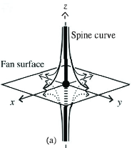
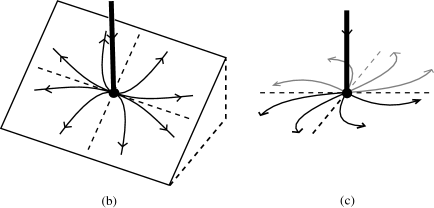
Figure 1: (a) The nature of magnetic field lines near a null point in 3D with a spine and a fan, for (a) a proper radial null, (b) an oblique null, and (c) a spiral null (from Priest[34] with permission).

The most general form of a linear null, for which the field components increase linearly away from the null, may be written [42]

$$\left(\begin{array}[]{c}B_{x}\\ B_{y}\\ B_{z}\end{array}\right)=\left(\begin{array}[]{ccc}1&\frac{1}{2}(b-j_{\parallel})&0\\ \frac{1}{2}(b+j_{\parallel})&a&0\\ 0&j_{\perp}&-a-1\end{array}\right)\left(\begin{array}[]{c}x\\ y\\ z\end{array}\right).$$ (5)

This includes both oblique nulls, in which the spine and fan are no longer perpendicular, and spiral nulls, for which the field lines in the fan spiral inwards or outwards. Null points are common in the corona [43], where they often appear at the summit of a separatrix dome that lies above a region of photospheric parasitic polarity surrounded by a region of the opposite polarity (Fig.2a).

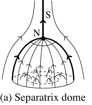
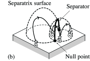
Figure 2: The topology of (a) a separatrix dome with a coronal null point N lying above a region of parasitic polarity and (b) two separatrix domes that intersect in a separator and lie above two sources of positive and two of negative polarity (from Priest[34] with permission).

The skeleton of a magnetic field consists of the separatrix surfaces (or separatrices), across which the mapping of field lines from their footpoints in the solar surface is discontinuous. Such separatrices originate either in so-called bald patches, where the magnetic field touches the boundary [44], or, more usually, at the fans of null points. Separatrices intersect in special field lines called separators that usually link one null point with another. Such separators were first considered by Sweet[15] and later analyzed by many others [14, 41, 45, 46]. An example is shown in Fig.2b, where four flux sources (two positive and two negative) in the solar surface produce two separatrix domes that originate as the fans of two null points, also lying in the solar surface, and the domes intersect in the separator. The skeleton can therefore be mapped out by determining the null points, the fan surfaces and the separators, an efficient method for which has been developed by Haynes et al.[47].

The quasi-skeleton, in contrast, consists of quasi-separatrix layers (QSLs) [48], which are surfaces across which the gradient of the mapping of field lines from one footpoint to another (Eq.6) is not singular but is very large. If a weak uniform field is added to a field with separatrices, the null points become locations where the field is weak but non-vanishing and the remnants of the separatrices become QSLs. The QSLs intersect in quasi-separators and are best diagnosed by mapping out the regions where the so-called squashing degree $Q$ is large, defined as follows [18]. First, split the surface of the volume under consideration into parts $S_{0}$ and $S_{1}$ where the field lines enter the volume at points $(x_{0},y_{0})$ and leave it at $(x_{1},y_{1})$ in cartesian coordinates. Then, the displacement gradient tensor is formed from the gradients of the mapping functions $x_{1}(x_{0},y_{0})$, $y_{1}(x_{0},y_{0})$ as

$${\bf\cal{F}}=\left(\begin{array}[]{ll}\partial x_{1}/\partial x_{0}&\partial x_{1}/\partial y_{0}\\ \partial y_{1}/\partial x_{0}&\partial y_{1}/\partial y_{0}\end{array}\right),$$ (6)

while $Q$ is defined as

$$Q=-\frac{B_{z+}}{B^{*}_{z-}}\left[\left(\frac{\partial x_{1}}{\partial x_{0}}\right)^{2}+\left(\frac{\partial x_{1}}{\partial y_{0}}\right)^{2}+\left(\frac{\partial y_{1}}{\partial x_{0}}\right)^{2}+\left(\frac{\partial y_{1}}{\partial y_{0}}\right)^{2}\right]$$ (7)

where $B_{z+}(>0)$ and $B^{*}_{z-}(<0)$ are the normal components of the field at the two ends of a field line. The region around a quasi-separator where Q is highest is called a hyperbolic flux tube (HFT) [18]. It is bounded by a flux surface $Q=\mbox{const}\gg 1$ with a shape that continuously changes along the HFT from a narrow flattened tube to a cross and then to a another narrow flattened tube at the other end and perpendicular to the first one, as follows [18]:

$$\begin{picture}(125.0,8.0)(0.0,0.0)\put(0.0,0.0){\line(1,1){10.0}}\put(-0.3,0.0){\line(1,1){10.0}}\put(-0.6,0.0){\line(1,1){10.0}}\put(-0.9,0.0){\line(1,1){10.0}}\put(-1.2,0.0){\line(1,1){10.0}}\put(-1.5,0.0){\line(1,1){10.0}} \put(14.0,2.0){$\rightarrow$} \put(28.15,2.0){$\times$}\put(27.87,2.0){$\times$}\put(27.59,2.0){$\times$}\put(27.31,2.0){$\times$}\put(27.03,2.0){$\times$} \put(28.0,0.0){\line(1,1){10.0}}\put(27.7,0.0){\line(1,1){10.0}}\put(27.4,0.0){\line(1,1){10.0}}\put(27.1,0.0){\line(1,1){10.0}}\put(26.8,0.0){\line(1,1){10.0}}\put(26.5,0.0){\line(1,1){10.0}} \put(42.0,2.0){$\rightarrow$} \put(56.0,0.0){\line(1,1){10.0}}\put(55.7,0.0){\line(1,1){10.0}}\put(55.4,0.0){\line(1,1){10.0}}\put(55.1,0.0){\line(1,1){10.0}}\put(54.8,0.0){\line(1,1){10.0}}\put(54.5,0.0){\line(1,1){10.0}} \put(66.0,0.0){\line(-1,1){10.0}}\put(65.7,0.0){\line(-1,1){10.0}}\put(65.4,0.0){\line(-1,1){10.0}}\put(65.1,0.0){\line(-1,1){10.0}}\put(64.8,0.0){\line(-1,1){10.0}}\put(64.5,0.0){\line(-1,1){10.0}} \put(71.0,2.0){$\rightarrow$} \put(95.0,0.0){\line(-1,1){10.0}}\put(94.7,0.0){\line(-1,1){10.0}}\put(94.4,0.0){\line(-1,1){10.0}}\put(94.1,0.0){\line(-1,1){10.0}}\put(93.8,0.0){\line(-1,1){10.0}}\put(93.5,0.0){\line(-1,1){10.0}} \put(85.15,2.0){$\times$}\put(84.87,2.0){$\times$}\put(84.59,2.0){$\times$}\put(84.31,2.0){$\times$}\put(84.03,2.0){$\times$} \put(100.0,2.0){$\rightarrow$} \put(124.0,0.0){\line(-1,1){10.0}}\put(123.7,0.0){\line(-1,1){10.0}}\put(123.4,0.0){\line(-1,1){10.0}}\put(123.1,0.0){\line(-1,1){10.0}}\put(122.8,0.0){\line(-1,1){10.0}}\put(122.5,0.0){\line(-1,1){10.0}} \end{picture}.$$

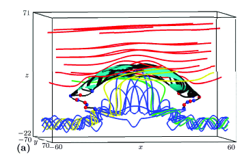
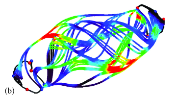
Figure 3: A numerical simulation for the emergence of a flux tube through the solar surface, showing (a) magnetic field lines viewed from the side, with separators (thick black lines) linking nulls, and (b) the separators and nulls viewed from above (from Parnell et al.[49] with permission).

Note that maps of Q will reveal both the skeleton and quasi-skeleton, but do not distinguish between them, and so, in order to isolate the quasi-skeleton, one needs first to determine the skeleton separately. Indeed, there are often more null points and separators in configurations than are intuitively expected. For example, a computational experiment on new magnetic flux emerging through the photosphere possessed 18 nulls and 229 separators [49] (Fig.3).

An important topological quantity in 3D reconnection studies is the magnetic helicity, part of which (the self-helicity) represents the twisting and kinking of flux tubes, while the remainder (the mutual helicity) measures the linkage between flux tubes. Its significance lies in the fact that it is conserved in an ideal medium and decays extremely slowly in a resistive one, so that only a very small change takes place in a reconnection event [50]. Thus, its approximate conservation is a constraint on the evolution of coronal magnetic fields [51].

For a magnetic field ${\bf B}={\bm{{\bm{\nabla}}}}\times{\bf A}$, a gauge-invariant expression for the relative magnetic helicity [52] inside a volume V bounded by a surface S is given by

$$H=\int_{V_{\infty}}({\bf A\cdot B-A}_{0}\cdot{\bf B}_{0})\;dV,$$ (8)

where ${\bf B}_{0}={\bf{\bm{\nabla}}\times A}_{0}$ is current-free inside $V$, with ${\bf B}_{0}={\bf B}$ outside $V$ and ${\bf A\times n=A}_{0}\times{\bf n}$ on $S$. Its rate of change due to motions on a boundary (S) is

$$\frac{dH}{dt}=-2\int_{V}({\bf j\cdot B}/\sigma)\;dV+2\int_{S}[({\bf B\cdot A}_{p})({\bf v\cdot n)-(v\cdot A}_{p})({\bf B\cdot n})]\;dS,$$ (9)

when the gauge (${\bf A}_{p}$) is chosen such that ${\bm{{\bm{\nabla}}}}\cdot{\bf A}_{p}=0$ and ${\bf A}_{p}\cdot{\bf n}=0$ on S. The first term represents helicity dissipation, which is very small, while the others give the transport of helicity through the surface, the first by flux emergence and the second due to footpoint motion.

Later, by extending earlier ideas of Berger[53], Yeates & Hornig[54] proposed a new topological flux function (the field line helicity) for magnetic field lines that connect two boundaries:

$${\cal A}=\int{{\bf A}\cdot}d{\bf s},$$ (10)

with the integral being taken from one end of a field line to the other end. It is an ideal invariant and measures the average poloidal flux around a field line. Its integral over one of the boundaries gives the relative magnetic helicity of the volume. It was applied to the evolution of coronal magnetic fields and shown to be concentrated in flux ropes [55].

2.3 Conditions for Reconnection

In an ideal plasma, when $R_{m}\gg 1$, Ohm’s law and its curl, namely, the induction equation, become

$${\bf E}+{\bf v}\times{\bf B}=\bf 0$$ (11)

and

$$\frac{\partial{\bf B}}{\partial t}={\bm{{\bm{\nabla}}}}\times({\bf v}\times{\bf B}),$$ (12)

which implies that both magnetic flux and magnetic field lines are conserved, i.e., plasma elements that form a flux tube or are joined by a field line will continue to do so.

However, in a non-ideal plasma, although flux conservation implies field-line conservation, the opposite is not true. Suppose in this case Ohm’s Law takes the form

$${\bf E}+{\bf v}\times{\bf B}={\bf N},$$ (13)

with a general nonideal term ${\bf N}$. A variation of a magnetic field then preserves magnetic flux if a magnetic flux velocity (${\bf w}$) exists that satisfies

$$\frac{\partial{\bf B}}{\partial t}={\bm{{\bm{\nabla}}}}\times({\bf w}\times{\bf B}),$$ (14)

for which Faraday’s law ($\partial{\bf B}/\partial t=-{\bm{{\bm{\nabla}}}}\times{\bf E}$) implies that ${\bf N}$ must have the form

$${\bf N}={\bf u}\times{\bf B}+{\bm{\nabla}}\Phi,$$ (15)

where ${\bf u}={\bf v}-{\bf w}$ is the slippage velocity and $\Phi$ is a potential. The presence of $\Phi$ can lead to a component ($E_{\parallel})$ of ${\bf E}$ along the magnetic field which is associated with 3D reconnection.

Comparing Eqns. (13) and (15), we see that

$${\bf E}+{\bf w}\times{\bf B}={\bm{\nabla}}\Phi,$$ (16)

so that, if ${\bf u}\cdot{\bf B}=0$, the flux velocity may be written

$${\bf w}={\bf v}+\frac{({\bf N}-{\bm{\nabla}}\Phi)\times{\bf B}}{B^{2}},$$ (17)

which tends to be singular at null points.

The condition for reconnection depends on the nature of the non-ideal term ${\bf N}$ in Eq.(13), as follows [56]:

(a) if ${\bf N}={\bf u}\times{\bf B}+{\bm{\nabla}}\Phi$, ${{\bf u}}$ is smooth, and there is no reconnection, but the magnetic field slips through the plasma;

(b) if ${\bf N}={\bf u}\times{\bf B}+{\bm{\nabla}}\Phi$ and ${\bf u}$ is singular, then reconnection occurs in 2D;

(c) if ${{\bf N}}\neq{\bf u}\times{\bf B}+{\bm{\nabla}}\Phi$, then reconnection occurs in 2.5D or 3D.

In case (a) there is a unique smooth flux velocity ${\bf w}$ which describes the transport of field lines by a unique smooth flow that preserves the field line topology. However, in 3D reconnection at an isolated diffusion region, there is no unique ${\bf w}$, and so two flux velocities (${\bf w}_{in}$ and ${\bf w}_{out}$) are needed to describe the behaviour of field lines, depending on whether the field lines are regarded as attached to the plasma in the ideal region on the side of the diffusion region where they enter or where they leave. For the Parker braiding problem or for quasi-separator reconnection, the flux velocity is non-unique but smooth, whereas for null-point or separator reconnection it is non-unique and non-smooth.

2.4 Reconnection in 3D versus 2D

The nature of reconnection in 3D is completely different from 2D, since most of the basic properties of 2D reconnection do not carry over into 3D [13]. By “2D reconnection" we mean reconnection in a strictly two-dimensional field ($B_{x}(x,y),B_{y}(x,y)$) that varies in two dimensions, whereas “3D reconnection" refers to reconnection in a fully 3D field ($B_{x}(x,y,z),B_{y}(x,y,z),B_{z}(x,y,z)$). Thus, 2D should not be confused with 2.5D, which we do not treat here and which refers to a field of the form ($B_{x}(x,y),B_{y}(x,y),B_{z}(x,y)$) with a guide field ($B_{z}(x,y)$). A 2D null point is topologically stable in 2D, in the sense that, if a purely 2D perturbation is made, the null point will continue its existence and just move its location slightly in 2D. Similarly, a 3D null point is also topologically stable. However, a 2.5D field, which exists in 3D, can be topologically unstable: for example, when a general 3D perturbation is made to a 2.5D X-line (consisting of a continuum of 2D X-points stacked on top of one another), it does not remain as an X-line but breaks up into a pair of 3D null points. There have been many very useful theories and simulations in 2D and 2.5D, which have helped to clarify our understanding of reconnection, but most examples in nature are three-dimensional and so the 2D and 2.5D understanding is often likely to be only partial.

In 2D, the properties are:

(i) Reconnection takes place only at X-type null points, where the magnetic field vanishes and the nearby field has a hyperbolic structure;

(ii) Magnetic flux moves at the flux velocity (${\bf w}$), which is singular at the X-point;

(iii) The mapping of field lines near an X-point from one footpoint to another is discontinuous as the footpoint crosses a separatrix;

(iv) During their passage through the diffusion region, field lines preserve their connections, except at the X-point, where they break and change their connections;

(v) When part of a flux tube is passing through a diffusion region, its two wings outside the diffusion region move with the plasma (${\bf w}={\bf v}$), while the segment inside the diffusion region slips through the plasma (${\bf w}\neq{\bf v}$).

In contrast, the properties of 3D reconnection are

(i) Reconnection occurs at null points, but also at separators and quasi-separators;

(ii) In general the notion of a flux tube velocity (${\bf w}$) fails;

(iii) At null points, separatrices and separators, the mapping of field lines from one boundary to another is discontinuous, but at quasi-nulls, quasi-separatrices and quasi-separators it is continuous;

(iv) During their passage through a diffusion region, field lines change their connections continually;

(v) When a field line is partly in the diffusion region, with one end moving with the plasma, the other end flips through the plasma with a velocity that is different from the plasma velocity.

In 3D, reconnection is defined as a change in the magnetic connectivity of plasma elements and, in terms of the electric field component ($E_{\parallel}$) parallel to the magnetic field, it may be diagnosed by the condition

$$\int E_{\parallel}\neq 0,$$ (18)

so that the electric field is non-zero along a magnetic field line that is reconnecting [11, 12].

Suppose Ohm’s law holds and the plasma flow vanishes on the boundary. Then the change of magnetic helicity (Eqn.9) becomes

$$\frac{dH}{dt}=-2\int{\bf E}\cdot{\bf B}\ dV,$$

but ${\bf E}\cdot{\bf B}=0$ outside the diffusion region $D_{R}$, and so this reduces to

$$\frac{dH}{dt}=-2\int_{D_{R}}E_{\parallel}B\ dV.$$

Thus, the condition for the magnetic helicity to change in time is identical to the condition that 3D reconnection exists. However, this change in magnetic helicity is extremely tiny compared with the total magnetic helicity present, so that, to a high degree of approximation, the total magnetic helicity remains constant.

The reason that nulls, separators and quasi-separators are associated with reconnection at diffusion regions that surround them is that they are natural locations where strong currents form. The consequences of reconnection are magnetic flipping and counter-rotation of field lines caused by a very small change of magnetic helicity. Other possible physical effects are acceleration of plasma jets by the resulting strong Lorentz forces, heating of plasma by Ohmic heating, and, beyond resistive MHD, acceleration of fast particles by the resulting strong electric fields, turbulence and shock waves.

2.5 Null-Point Reconnection: Theory

Reconnection can occur in three main ways at a null point, depending on the nature of the flows that are present. The most common form of null-point reconnection is spine-fan reconnection [57], produced by shearing motions that produce flows across both the spine and fan of the null. On the other hand, twisting motions can produce either torsional spine reconnection or torsional fan reconnection. These modes of reconnection were discovered on the basis of kinematic models and computational experiments.

Steady-state kinematic models for the ideal region may be set up by solving

$${\bf E}+{\bf v}\times{\bf B}={\bf 0}\ \ \ {\rm and}\ \ \ {\bm{{\bm{\nabla}}}}\times{\bf E}={\bf 0},\ \ \$$ (19)

for the velocity ${\bf v}$ and electric field ${\bf E}={\bm{\nabla}}\Phi$ with a given magnetic field containing a null point [41]. Corresponding models for an isolated diffusion region were set up by Hornig & Priest [58] by solving Ohm’s law

$${\bf E}+{\bf v}\times{\bf B}=\eta\ {\bm{{\bm{\nabla}}}}\times{\bf B}.$$ (20)

The component of Eqn.(20) along the magnetic field gives the potential $\Phi$ everywhere as

$$\Phi=\int\frac{\eta\ {\bf j}\cdot{\bf B}}{B}\ ds+\Phi_{e},$$ (21)

namely, an integral along field lines in terms of the imposed value ($\Phi_{e}$) at one end. The component of Ohm’s law normal to the magnetic field then determines the flow component ${\bf v}_{\perp}$ normal to the magnetic field as

$${\bf v}_{\perp}=\frac{({\bm{\nabla}}\Phi-\eta\ {\bf j})\times{\bf B}}{B^{2}},$$ (22)

while the rate of change of magnetic flux ($F_{m}$) (i.e., the reconnection rate) follows from

$$\frac{dF_{m}}{dt}=\int E_{\parallel}ds.$$ (23)

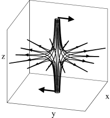
(a) (b)

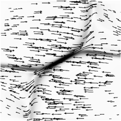
Figure 4: (a) An initial shearing in the $y$-direction of a spine aligned with the $z$-axis. (b) The resulting collapse of spine and fan to form spine-fan reconnection, showing the current-density contours (shaded) and flow velocity arrows in the $x=0$ plane (from Pontin & Galsgaard[59] with permission).

Pontin et al. [60] applied the above approach to a diffusion region in the shape of a disc containing a uniform current along the fan. They found that the plasma flow crosses both the spine and fan. The field lines flip up and down the spine and around the spine in the plane of the fan. A numerical solution of the full resistive MHD equations by Pontin & Galsgaard [59] showed how a shearing of the spine drives such spine-fan reconnection (Fig. 4) with a strong fan current.

The kinematic formalism may also be applied to a spiral null with a cylindrical diffusion region. Rotation of the fan plane then tends to drive current along the spine and create twisting motions around the spine in torsional spine reconnection. Inside the diffusion region, rotational slippage allows the field lines to become disconnected and to rotate around the spine. On the other hand, rotation of the region around the spine in opposite directions above and below the null drives a strong fan current in torsional fan reconnection. In this case, inside the diffusion region the field lines exhibit rotational slippage above and below the fan plane.

2.6 Separator Reconnection: Theory

In complex magnetic fields, null points are common and the particular magnetic field line where the fans of two nulls intersect, called a separator, is a prime location for the build up of currents and therefore for reconnection. For example, the configuration with magnetic field

$$B_{x}=x(z-3),\\ \ B_{y}=y(z+3),\ \ \ B_{z}=1-z^{2}$$

has two nulls. As indicated in Fig. 5, one null at $(0,0,-1)$ has its fan orientated in the $yz$-plane, while the other at $(0,0,1)$ has a fan in the $xz$-plane, so that these two fans intersect in the $z$-axis.

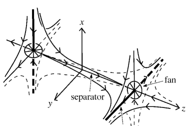
Figure 5: An example of a separator that joins two nulls (from Priest[34] with permission).

In two pioneering papers Sweet [15], Lau and Finn [14] suggested that current sheets can form along separators and lead to reconnection, an idea later developed by others [41, 45, 61]. A series of computational experiments by Parnell, Longcope and their colleagues demonstrated the importance of separator reconnection in coronal heating and in solar flares, as described in Sec.33.2. Furthermore, the relation between separators and quasi-separators was clarified [62], by showing that spines and certain portions of fans are good predictors for QSL footprints and flare ribbons.

For a topologically complex magnetic field, Parnell et al. [63] discovered the importance of analyzing the skeleton of separatrix surfaces that spread out from the fans of the null points. This enabled them to determine how multiple reconnecting separators can be born joining the same two null points, and how in recursive reconnection the same flux can be closed and opened many times. Later, Parnell et al. [46] were surprised to find that the magnetic field in a plane perpendicular to a separator can be either hyperbolic (X-type), as expected, or elliptic (O-type), and that this may vary along the separator, with reconnection occurring at both types of structure.

Longcope [64] also studied how separator current sheets form and dissipate. He demonstrated how the current and energy storage are produced by a change in magnetic flux, and applied the ideas to X-ray bright points [65] and to solar flares [66].

More recently, in order to develop a new model for coronal heating by flux cancellation, Priest & Syntelis [67] developed a method to calculate 2D and axisymmetric 3D separator current sheets and their reconnecting properties without resorting to complex variable theory.

2.7 Quasi-Separator Reconnection: Theory

As described in Sec.22.2, quasi-separators or hyperbolic flux tubes are intersections of quasi-separatrices, which are regions where the mapping gradient (Eq.6) or squashing degree ($Q$, Eq.7) is not infinite but is much larger than unity. Since they may often be regarded as remnants of separators, it is not surprising that current sheets will tend to form at them and so reconnection is likely to take place [48].

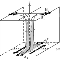
Figure 6: An example of a quasi-separator (from Priest[34] with permission).

Consider, for example, a magnetic field with cartesian components $(x,-y,\epsilon)$, consisting of a uniform $z$-component of magnitude $\epsilon\ll 1$ superposed on an X-point field in $xy$-planes (Fig.6). The field line that maps a point B$(x_{1},y_{1},1)$ on the plane $z=1$ to A$(x_{0},y_{1},0)$ on the plane $z=0$ is given by

$$x_{0}=x_{1}\exp(-1/\epsilon),\ \ \ \ y_{0}=y_{1}\exp(1/\epsilon).$$

Thus, the mapping is continuous, but suppose B moves from B₁ to B₂ across the $x$-axis with $x_{1}$ fixed and positive, while $y$ increases from a small negative value at B₁ to a small positive value at B₂. Then A will move from a large negative value at A₁ to a large positive value at A₂. On the other hand, if $x_{1}$ is fixed and negative, A will move in the opposite direction. In other words, small motions of the footpoints on the top boundary across the QSL (the $xz$-plane) produce extremely rapid flipping of the feet on the bottom boundary. When magnetic reconnection occurs within QSLs in 3D, field lines exchange their connectivity with those of their neighbours in the reconnection layer, and the magnetic field lines flip (or slip or slip-run) past each other at super-Alfvénic speeds [19, 16, 68]. Physically, therefore, the behaviour of quasi-separator reconnection and separator reconnection is very similar on MHD time scales.

Indeed, Démoulin et al. [17] showed that, if a quasi-separator is present in the corona, the effect of any smooth motion of the photospheric footpoints will be to create a current sheet there. Also, Titov et al. [69] demonstrated that a stagnation-point flow near a QSL generates strong currents near it, while Aulanier et al. [70] and others confirmed the effect with resistive numerical experiments (see Sec.33.3).

3 Modelling and Observations of 3D Magnetic Reconnection

3.1 Null-Point Reconnection: Modelling and Observations

3D null points as described in Sec.22.2 are preferential sites for current accumulation and energy dissipation. They have been observed directly in the Earth’s magnetosphere in the magnetotail[71, 72] and the polar cusp region[73] (Sec.3a3.1.2). They are also abundant in the solar atmosphere and a common feature of solar flares[74], CMEs[75], solar jets[76, 77] and flux emergence[78] (Sec.3a3.1.1). In particular, they arise commonly when parasitic polarity surrounded by opposite polarity of greater flux forms a coronal null [79], whose fan takes the shape of a separatrix dome (Fig.2a).

Spine-fan reconnection (Sec.22.5) has been studied in MHD simulations by Pontin et al.[80], who demonstrated that magnetic collapse near a null forms a current sheet localized around it. Flipping (or slipping or slip-running) of field lines then occurs during the spine-fan reconnection, with the magnetic connectivity of field lines continually changing [68] and flux being transferred between topologically different domains (Fig.7). The flipping velocity becomes infinite on field lines that pass through the null itself.

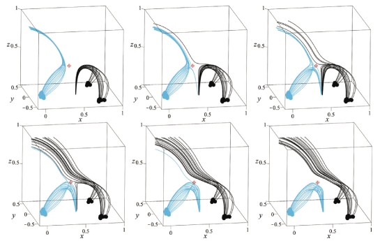
Figure 7: Flux transfer for spine-fan reconnection at a null point (the red diamond), with blue and black lines traced from fixed footpoints. Blue field lines initially outside the separatrix surface are transferred to inside the separatrix, while black field lines inside the separatrix are moved to outside the separatrix (from Pontin et al.[80] with permission).

3.1.1 Null Points and Solar Flares

Null-point reconnection is thought to play a key role in many solar flares, especially circular-ribbon flares [81, 82]. Recent observations and 3D simulations show that when a magnetic bipole emerges into a unipolar region, reconnection between the two fields forms a coronal null configuration (with a 3D fan-spine structure) in the corona[79, 83]. Null-point reconnection then generates heat and fast particles, which travel along the fan separatrix and light up the fan footpoints to form circular ribbons [84] (Fig.8). In addition, a central ribbon and a remote ribbon are observed at the footpoints of the spines that are located below and above the dome, respectively.

Magnetic extrapolations of the photospheric field confirm that twisted flux ropes are often present under the fan surface [85]. When the flux rope loses equilibrium (due to nonequilibrium or kink or torus instabilities[86, 33]), the flux rope rises and triggers more violent null-point reconnection[87, 88]. Such flux rope eruption can generate a blowout jet[89], collimated from low down in the atmosphere [76].

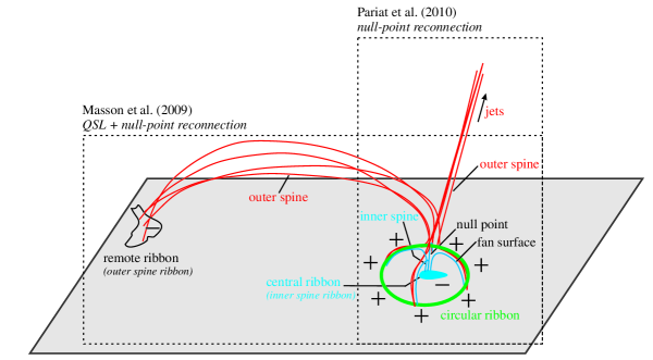
Figure 8: Schematic of the relationship between circular flare ribbons, jets, and remote brightenings in a 3D fan-spine magnetic topology (from Wang & Liu[84] with permission).

Circular flare ribbons often brighten sequentially in a clockwise or anti-clockwise direction [81, 90, 91]. For example, Li et al.[91] found circular ribbon elongation at a high speed of 220 km s^-1. It is a natural consequence of the flipping or slipping of magnetic field lines that occurs in null-point reconnection, as demonstrated by Pontin et al [80].

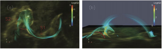
Figure 9: A good agreement between the location of flare ribbons in 1600 Å and values of Q for a potential field extrapolation. Red lines denote the skeleton structure of the null point. S1 and S2 represent the western and eastern structures surrounding the spine and fan field lines where Q is large (from Yang et al.[90] with permission).

Several authors have calculated the distribution of the squashing degree Q in configurations with coronal nulls or separators [81, 90] (Fig.9). Of course, Q is infinite at the separatrices, although methods to determine Q will just show it to be high rather than infinite, due to the finite resolution of the methods. Nevertheless, when nulls or separators are present, they give rise to null-point or separator reconnection rather than quasi-separator reconnection. Pontin et al.[92] clarified this point by showing that an extended high Q-halo around the spine or fan is a generic feature of null-point or separator reconnection. Thus, we stress that it is important to determine carefully whether there are any nulls or separators present before calculating Q, since by itself neither Q nor the presence of flipping will distinguish between the different types of reconnection. In addition, maps of Q will also show up structures away from the separatrices where the mapping gradient is large but where current sheets do not form.

Null-point or separator reconnection is also involved in the breakout mechanism proposed by Antiochos et al.[93] as a possible explanation for the initiation of some CMEs and eruptive solar flares in a quadrupolar configuration. In the breakout model, reconnection between a low-lying sheared core flux and a large-scale overlying flux system enables the core flux to "break out". Later, the model was extended to a fully 3D system, with two polarity inversion lines, a separatrix dome and a 3D null point at the intersection of the separatrix surface and the spine field lines[75]. The mechanism has also been used to explain small-scale solar jets [76, 94].

3.1.2 Null Points in Earth’s Magnetosphere

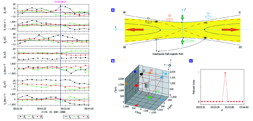
Figure 10: In situ observations of a magnetic null point by four Cluster spacecraft in a magnetotail reconnection region. (left) The magnetic field and plasma flow. (right) The Poincaré index is non-zero when the four spacecraft surround a null point. (From Xiao et al. [95] with permission.)

In situ measurements of 3D magnetic null points have been made in reconnection regions of the Earth’s magnetosphere (Fig. 10) [95], using observations from the four Cluster spacecraft. They are identified from the Poincaré index calculated from the observed magnetic vectors at four non-coplanar points that surround the null point. The eigenvalues and eigenvectors of the matrix $\delta B_{ij}=\nabla_{j}B_{i}$ are calculated assuming a linear interpolation and supposing there is only one null point in the tetrahedron obtained from the four spacecraft positions. He et al. [96] extended the method to include an arbitrary number of null points (Fig. 11). As a result, 3D null points have been identified in the Earth’s magnetotail [97, 98, 95], magnetopause [99], turbulent magnetosheath [100], and bow shock [101]. The spatial scale for variations of the magnetic field near the observed magnetic null is on the order of an ion inertial length [102], implying that the Hall effect is important.

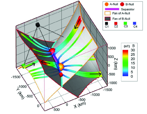
Figure 11: A separator reconnection configuration with a magnetic null pair reconstructed from Cluster measurements at 09:48:25.637 UT on Oct 1st, 2001, consistent with the analysis of Xiao et al. [98]. (From He et al. [102] with permission.)

Both spacecraft data and simulation results show that spiral null points tend to occur more often than radial null points [103, 104], regardless of the regions in the magnetosphere and the magnetosheath. The observations at ion scales show that spiral nulls are naturally related to twisted magnetic flux ropes [105, 106, 107], which may play an important role in plasma acceleration during 3D reconnection [108]. Indeed, energy dissipation is strong in outflow helical field lines [109] and in clusters of nulls [110]. The close relation between spiral nulls and flux ropes may well hold also at other scales.

Cluster spacecraft data allow one to measure the plasma velocity, plasma number density, electric field, and current flow near a null point, as well as its motion. Perpendicular plasma flows around a spiral null found by Wendel & Adrian [100] often rotate in the fan plane, especially when the fan or spine are approached. The current is mainly along the spine but also has a component perpendicular to the spine. The flows indicate a combination of torsional spine and fan reconnection, which was also observed in the magnetotail [105].

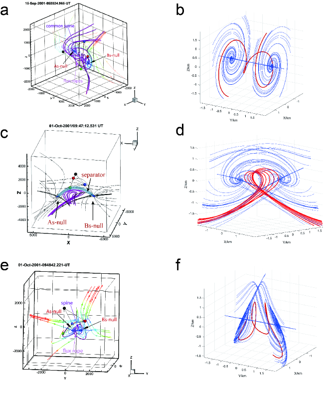
Figure 12: (left) Reconstruction of three types of spiral null pair observed by Cluster. (right) The configuration of the spiral null pairs based on the analytical model with (b) $\varepsilon=0$, $\alpha=0$, and $j=6$; (d) $\varepsilon=2$, $\alpha=3$, and $j=6$; (f) $\varepsilon=0$, $\alpha=3$, and $j=6$. (From Guo et al. [105] [106] with permission.)

Nulls may be generated in pairs [111] when a separator is born (see Secs.22.6,33.2). Spiral null pairs are sometimes related to the formation of flux ropes, when they are chained by helical field lines along their spines. This structure has been observed in the magnetotail by Cluster [105] and in solar emerging flux simulations [49]. Fig. 12 gives the reconstructed magnetic structure for three different spiral null pairs. In each case an As-type null is joined to a Bs-type null (Sec.22.2). In Fig. 12a the nulls are linked by their spine lines, which could be a common spine or more likely two helically wrapped spine lines, since the former is topologically unstable. Field lines around the spines and between the two spiral nulls are twisted to form flux ropes. Such structures are also found in simulation results [104], which show that the spiral nulls are formed by the wrapping and kinking of a current sheet.

In Figs. 12c and 12e the nulls are connected by a separator and by both spine and separator [106], respectively. These two structures, which were observed in the magnetotail, as well as the As-spine-Bs-like case can be represented by the following magnetic field [106]:

$$(B_{x},B_{y},B_{z}\ )=[xy-\textstyle{\frac{1}{2}}\ jz+\varepsilon y,1-y^{2}+\alpha x,\ zy+\textstyle{\frac{1}{2}}\ jx].$$

In this analytical model, the two spiral nulls are located along the $y$-axis and $j$ is the current density along the $y$-axis. The terms $\varepsilon y$ and $\alpha x$ represent magnetic perturbations parallel and perpendicular to the line joining the nulls. The plots in the right column of Fig. 12 give three types of null pairs by choosing different values for $\varepsilon$ and $\alpha$. In each structure, the flux ropes are formed between two spiral nulls and surround the spine lines. These different linkages between spiral null points could be generated by different bifurcation processes produced by different magnetic perturbations in time and space [112].

The formation, disappearance and bifurcation of null points frequently takes place during 3D reconnection. As observed in the magnetotail, the number of null points in the region enclosed by four Cluster spacecraft can vary rapidly, presenting a turbulent-like reconnection region [110]. In a turbulent plasma, the dissipation is largely produced by reconnection at clusters of null points and short-lived radial null pairs and at the separators joining the nulls [49].

3.2 Separator Reconnection: Modelling and Observations

Separator reconnection is widely thought to be important in coronal heating, solar flares, and the Earth’s magnetosphere, as described below (Secs. 3b3.2.2,3b3.2.3,3b3.2.4). But first we give examples of local and global skeletons of coronal magnetic fields constructed from photospheric magnetograms (Sec.3b3.2.1).

After the crucial importance of analysing the skeleton of separatrix surfaces was realised [113], Parnell and Longcope [63, 49, 47, 114, 66] developed the necessary techniques and applied them to numerical experiments and observed magnetic fields. The importance of the skeleton and its evolution is that it reveals the different topological regions and how they evolve by separator reconnection, as well as how the separators are born, evolve, and disappear. Later, Titov [115, 116] generalised this concept to that of a structural skeleton, which is the sum of the skeleton and quasi-skeleton of quasi-separatrices (Sec.33.3).

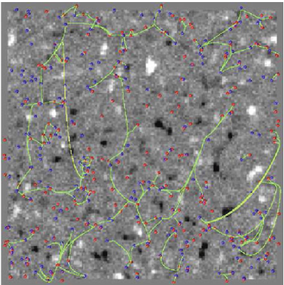
Figure 13: Local skeleton from a potential field extrapolation above a photospheric magnetogram of a small part of the solar surface from SOHO/MDI, together with the positive nulls (red dots) and negative (blue dots) nulls and separators (green curves). The observed photospheric magnetic field is of mixed polarity and highly fragmented and is known as the Magnetic Carpet. (From Parnell et al.[117] with permission.)

3.2.1 Skeletons from Photospheric Magnetograms

The results from an early potential field extrapolation of a local photospheric magnetogram from SOHO/MDI are shown in Fig. 13, revealing the presence of many null points produced by the highly localised and mixed-polarity nature of the magnetic flux protruding through the solar surface, known as the magnetic carpet [118].

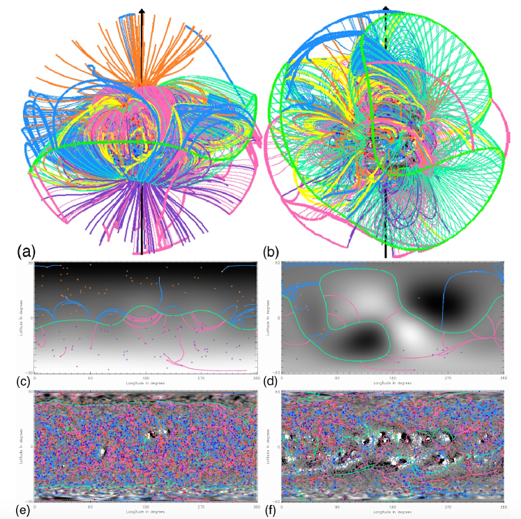
Figure 14: Global skeleton from a potential field extrapolation above a synoptic photospheric magnetogram of the whole of the solar surface at (a) solar minimum and (b) solar maximum. The topological features are the positive nulls (red dots) with spines (purple) and separatrices (thin pink lines), negative nulls (blue dots) with spines (orange) and separatrices (thin blue lines), spines, and separators (green curves). Thick pink and blue lines denote where the separatrices meet the source surface ($r=2.5R_{\odot}$), whereas thick green lines mark the base of the heliospheric current sheet and thin green lines extending down from them map out the heliospheric current sheet curtains dividing open and closed fields. (c) and (d) show cuts at a radius $r=2.5R_{\odot}$, while (e) and (f) show cuts at $r=1.005R_{\odot}$ as well as all the null points. (From Parnell et al.[119] with permission.)

Later, the global coronal topology at solar minimum and solar maximum was calculated (Fig. 14) using SOLIS synoptic magnetograms and a global potential field model with a maximum harmonic number of $l=301$ to extrapolate the magnetograms. The global study by Platten et al. [120] revealed 1964 nulls and 1946 separators at solar minimum, but 1131 nulls and 808 separators at solar maximum. During solar minimum there are large areas of the photosphere with small-scale mixed polarity that create a highly complex network of nulls and separatrices (Fig. 14e).

Note that, for both local and global skeletons, much greater complexity with many more nulls and separators would be produced if much higher-resolution extrapolations from more recent magnetograms from SDO and the SUNRISE balloon were undertaken.

3.2.2 Separators and Coronal Heating

Coronal heating due to several effects has been proposed. The idea that the corona is filled with myriads of current sheets that are continually forming and reconnecting to give nanoflares was proposed by Parker [121] and has traditionally been modelled in terms of braiding an initially uniform magnetic field by footpoint motions [122, 123].

However, the flux tube tectonics model [124] suggested that the magnetic carpet is crucial, since it highlights the fact that the photospheric sources of coronal magnetic field are not smoothly varying large-scale structures, but are instead highly concentrated and localised magnetic fragments and intense flux tubes (Figs.13,14). The fact the magnetic flux protrudes through the solar surface into the corona at many small highly concentrated locations makes the chromospheric and coronal magnetic field highly complex with myriads of null points (or quasi-nulls) and separators (or quasi-separators) at which current sheets can form and reconnection takes place [125, 126].

Thus, flux tube tectonics may be regarded as a modern development of Parker’s nanoflare heating ideas which leads to much more efficient heating, since it considers the action not of complex photospheric motions on a uniform field but of simple motions on a magnetic field that observations imply is highly complex.

A key way in which coronal tectonics heats the corona has been modelled in a pioneering numerical experiment by Parnell, Galsgaard and Haynes [122, 61, 127, 47, 46]. They consider an elementary interaction between two photospheric magnetic sources, in which one flux source moves past another flux source of opposite polarity in the presence of an overlying horizontal magnetic field that is so-called flyby. They found that, if the separation of the sources is small enough, reconnection is driven at a series of separators.

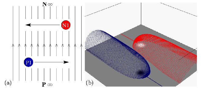
Figure 15: Initial setup for a numerical flyby experiment showing (a) the view from above and (b) the magnetic skeleton. (From Parnell & Haynes[128] with permission.)

Fig. 15a shows the initial set up for Parnell’s numerical experiment, with two photospheric flux sources of opposite polarity ($P1$ moving to the right and $N1$ moving to the left) in an overlying uniform field that is perpendicular to the motion of the sources. Figure 15b gives the initial magnetic skeleton, in which the two sources are not joined. There are two null points in the photosphere, with fans that form two open separatrix surfaces extending along the direction of the overlying field. Below the blue separatrix all the flux from the positive source extends out through one side boundary, while below the red surface the flux from the negative source extends out through the opposite boundary. These fluxes are designated by the adjective open, whereas the flux that later links one source to the other is called closed.

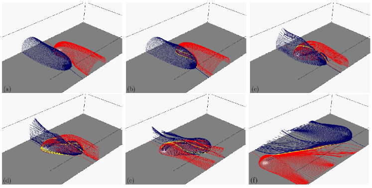
Figure 16: The evolution of the skeleton for the flyby experiment, namely, the interaction of the two separatrix surfaces (red and blue) with separator field lines shown in yellow. (From Parnell & Haynes[128] with permission.)

Then Fig. 16 shows the subsequent evolution of the skeleton, in which the two separatrices intersect in a number of reconnecting separators that vary as the simulation proceeds.

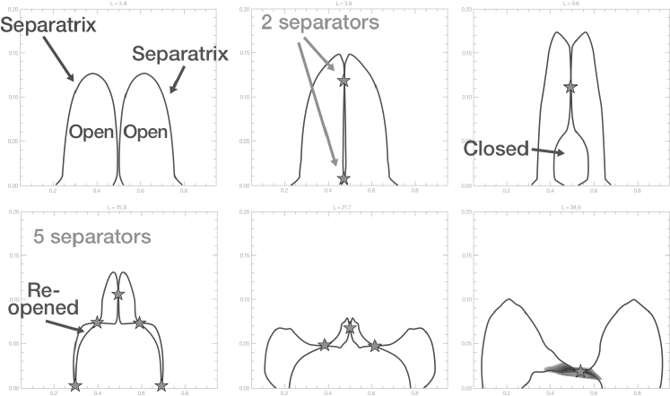
Figure 17: The evolution of the intersections with a vertical cross-section at the mid-plane $y=0.5$ for the flyby simulation of Fig.16. “Open" refers to flux that links one of the sources with a side boundary of the numerical box, while “Closed" denotes flux that joins the two sources. (From Priest [34] with permission.)

It is. however, by taking a vertical section through the skeleton that what is happening becomes clear (Fig. 17). Initially, the two separatrices are completely separate, and then they touch and intersect in two separators. One of these descends through the lower boundary to leave one separator, where reconnection builds up the closed flux linking the two sources. Next, the separatrix surface that bounds the closed region touches the side separatrices and intersects them to give four more separators, two on each side. Two of these descend through the lower boundary to leave the central separator and two side separators whose reconnection reopens part of the flux.

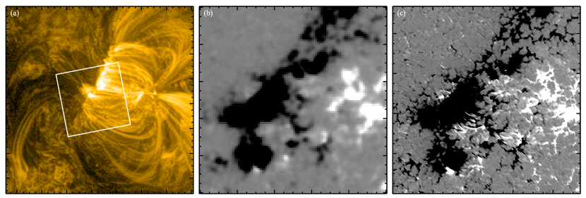
Figure 18: Coronal image of an active region on 2013 June 12 at 23:45 UT, and the underlying magnetic field. (a) An image from the SDO/Atmospheric Imaging Assembly (AIA) 171 Å filter in a 150x150 arcsec field of view. The white box covers an area of 51x51 arcsec and encloses footpoint regions of several coronal loops. (b) SDO/HMI magnetogram showing the distribution of the photospheric line of sight magnetic field for the white box region of panel (a). (c) Same as (b) but for the SUNRISE/IMaX observations. (From Priest et al. [129] with permission.)

Recent observations from the SUNRISE balloon mission [130] have revealed that the photospheric magnetic field is very much more complex than realised before and that magnetic flux in the Quiet Sun is emerging and cancelling at a rate of 1100 Mx cm^-2 day^-1 [131], which is an order of magnitude higher than thought before. Figs. 18a and b show an image of the corona and the underlying magnetogram from SDO/HMI, which implies that the feet of the coronal loops are unipolar. However, Fig. 18c gives the equivalent much higher-resolution magnetogram from SUNRISE, which reveals that the feet instead consist of many tiny regions of mixed magnetic polarity which are cancelling.

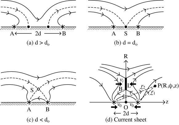
Figure 19: The flux cancellation model for coronal heating. (a) Two photospheric magnetic sources of flux $\pm F$, situated on the z-axis a distance $2d$ apart in an overlying uniform horizontal field $B_{0}$ approaching one another at speed $v_{0}$. (b) When $d=d_{0}$, a separator S is formed. (c) Reconnection is driven at the separator $S$ which rises in the atmosphere. (d) Energy is converted at a current sheet of length $L$, where plasma flows in at speed $v_{i}$ carrying magnetic field $B_{i}$. (From Priest & Syntelis [67]. Reproduced with permission from Astronomy & Astrophysics.)

This led Priest et al. [129] to propose a flux cancellation model for chromospheric and coronal heating by nanoflares that are created not by braiding reconnection in the corona but by reconnection driven by photospheric flux cancellation (Fig. 19). As a simple model of this process, they start with two opposite-polarity magnetic fragments of flux $\pm F$ in an overlying horizontal field $B_{0}$ and consider what happens as the half-distance $d$ between them decreases and eventually the fragments cancel (Fig. 19). Initially, $d$ is large and there is no flux joining one fragment to the other, but, when $d$ becomes smaller than the interaction distance [65]

$$d_{0}=\left(\frac{F}{\pi B_{0}}\right)^{1/2},$$ (24)

their fields start to reconnect at a separator. The length $L$ of the three-dimensional current sheet, as well as the inflow speed $v_{i}$ and magnetic field $B_{i}$, were calculated in terms of the speed ($v_{0}$) of approach of the fragments, their fluxes ($F$) and the overlying field strength ($B_{0}$).

The energy release occurs in two phases: in the first phase, as the fragments approach, the separator rises to a maximum height that depends on $d_{0}$ and then falls to the photosphere; in the second phase the fragments cancel. The maximum height of energy release can be located in the chromosphere, transition region or corona, depending on the parameter values, and in both cases energy is released as heat and as the energy of a hot fast jet, as well as fast particles. For observed parameter values, the energy release is sufficient to heat the chromosphere and corona and can account for a range of observed dynamic effects. More recently, the model has been supported and extended by an analysis of reconnection at a 3D separator current sheet [67], as well as by numerical simulations [132] and observations of heating in the core of active regions in bright loops with flux cancellation at their footpoints [133].

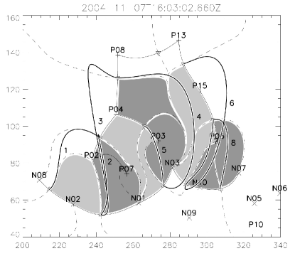
Figure 20: The footprint of the skeleton of an active region, indicating: sources that are positive (+) or negative ($\times$); null points that are positive (${\bm{\nabla}}$) or negative ($\bm{\Delta}$); spines (solid); footprints of fans (dashed); separators (thick curves); and domains that gain flux (dark) or lose flux (light). (From Longcope et al. [134] with permission.)

3.2.3 Separators and Solar Flares

Separator reconnection is also a prime explanation for many solar flares [135]. Longcope et al. [66, 136] have shown how in many flares the stored energy can be released by separator reconnection as it spreads through many domains of an active region, as described below.

Longcope et al. [134] predicted the flare energy release for several active regions and compared it favourably with observations. The coronal magnetic field is likely to evolve through a series of nonlinear force-free equilibria with current sheets along separators, but these are difficult to calculate, and so Longcope [64] developed a simpler Minimum Current Corona (MCC) model. In this model, the photospheric magnetic field is split into a series of positive (P_i) and negative (N_j) unipolar flux patches, and the flux in the domain joining P_i to N_j is calculated. The domains are bounded by separatrices, which intersect in separators and make up the configuration’s skeleton [137]. In practice, reconnection between domains would conserve the total magnetic helicity and so the field in each domain would be force-free, but, the MCC model assumes instead that the field evolves through a series of flux-constrained equilibria with the minimum energy that preserves the domain fluxes and with current sheets located along the separators. The free energy is then released by separator reconnection as flux is transferred between domains and the field is reduced to a potential one.

Longcope et al. [134] partitioned a particular active region up into 28 regions, whose initial skeleton is shown in Fig.20a. It has 29 nulls and 32 separators. They then calculated the changes in domain flux by a sequence of separator reconnections and so showed how reconnection spreads through the region. Flux changes are used to calculate the currents acting along each separator and also the energy released, which in this case amounts to $8\times 10^{31}$ erg, or 6$\%$ of the active-region energy. The flare ribbons are found to lie along a series of spines that join a set of nulls. Titov et al. [138] applied the same idea to the triggering of a sequence of flares and CMEs.

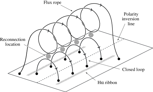
Figure 21: A 3D flare cartoon for the creation of an arcade of flare loops and a twisted flux rope by reconnection at many sites above a polarity inversion line. (From Longcope et al. [134] with permission.)

During a solar flare, 2D models suppose reconnection creates a closed field line or magnetic island, but 3D models instead imply that reconnection at a series of locations produces a twisted flux rope, as shown in Fig.21, together with coronal arcade of flare loops.

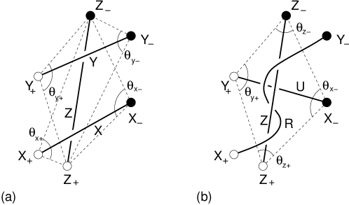
Figure 22: The creation of twist by the zippette process, namely, reconnection of two coronal loops ($X_{+}X_{-}$,$Y_{+}Y_{-}$) overlying a prominence flux tube ($Z_{+}Z_{-}$) to create a twisted flux rope $X_{+}Y_{-}$ whose core is $Z_{+}Z_{-}$. (From Priest & Longcope [139] with permission.)

A model for zipper reconnection by Priest & Longcope [139] has addressed two important questions about the three-dimensional aspects of a flare, namely: during the rise phase, how do two bright flare knots grow into ribbons while a single loop joining them develops into a flare arcade? and what is the nature and magnitude of the resulting twist in the erupting flux rope? Fig. 22a shows the zippette process in which two untwisted flux tubes (X₊X_- and Y₊Y_-) overlie an initial flux rope (Z₊Z_-), which reconnect below Z₊Z_- to create an underlying flux tube U from Y₊ to X_- together with a twisted flux rope R from X₊ to Y_- that wraps around Z₊Z_-.

Figure 23: A zipper model for the creation of flare ribbons and the build-up of twist in an erupting flux rope. (From Priest & Longcope [139] with permission.)

The idea in zipper reconnection (Fig.23) is then that, before the flare the magnetic configuration in an active region consists of an arcade of coronal loops (A₊A_-, B₊B_-, C₊C_-, D₊D_-) overlying a filament or prominence Z₊Z_-, whose magnetic field is a flux tube that may be untwisted or only weakly twisted (Fig.23a). Then the flare is initiated when reconnection starts at one point in the arcade, such as, e.g., at the lower end in Fig.23a. Then, during the rise phase, zippette reconnection first takes place between A₊A_- and B₊B_- to produce a flux rope A₊B_-, a flare loop B₊A_- and brightening at the feet A₊B₊ and A_-B_- as the start of the flare ribbons (Fig.23b). Next the reconnection spreads along the polarity inversion line, gradually filling up the flare arcade and the flare ribbons. First of all, A₊B_- reconnects with C₊C_- to create the twisted rope A₊C_- (Fig.23c), and later A₊C_- reconnects with D₊D_- to create A₊D_-. At the end of this process (Fig.23d), the ribbons and arcade of hot loops have been created, together with a highly twisted flux rope, whose core is the initial prominence field Z₊Z_- and whose main part is A₊D_-. Once the flare ribbons have formed during the rise phase by zipper reconnection, the ribbons move apart during the main phase as reconnection moves to higher locations in the usual way.

Later, Priest & Longcope [140] considered in detail the way twist is acquired by the 3D reconnection of two flux tubes and its distribution within the flux tubes. One constraint on this process is that the total magnetic helicity is conserved as mutual helicity is converted to self-helicity and so creates twist. However, both a local and a global aspect to the process are also present: the local effect is to produce equipartition of the amount of self-helicity and therefore twist that is added to the tubes; but the additional global effect implies that the location and orientation of the flux tube feet generally add extra different self-helicities to the two tubes.

Two extra effects that are present in separator reconnection, but which have been highlighted in quasi-separator studies are the presence of hooks at the ends of the flare ribbons and the occurrence of flipping or slipping of magnetic field lines. For more details, see Sec.33.3.

3.2.4 Separators in the Earth’s Magnetosphere

Separator reconnection is also critical in the interaction between the solar wind and the Earth’s magnetosphere. This is a huge field and so we are reviewing only a small portion of the literature here. Xiao et al. [98] showed for the first time through in situ observations how the separator of a null pair can serve as the location for reconnection. Also, the magnetic configuration was determined and a Hall electric field measured at the separator [102].

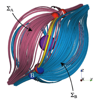
Figure 24: Magnetic skeleton computed from the OpenGGCM simulation. Type A (i.e., negative) nulls are shown as red spheres, while Type B (i.e., positive) nulls are indicated by blue ones. The thick yellow line lies approximately at the intersection of the two separatrix surfaces ($\Sigma_{A}$ and $\Sigma_{B}$). (From Dorelli et al. [141] with permission.)

A long-lasting debate about magnetopause reconnection concerns the location of the line where reconnection takes place. In 2.5D reconnection theory, two possibilities are antiparallel reconnection with no guide-field and component reconnection with a guide-field out of the 2D plane, but 2.5D is topologically unstable and so mention of antiparallel or component reconnection refers only to local behaviour without refence to the global 3D topology. A 3D MHD simulation performed by Dorelli et al. [141] with zero magnetic dipole tilt and an IMF (interplanetary magnetic field) clock angle of 45^∘ showed that null clusters form in two cusp regions connected by a separator that runs through the dayside magnetopause (Fig. 24), although such a separator is difficult to identify in in situ observations. The simulation possesses two types of reconnection. The first is null-point reconnection in the cusp null clusters and in the high-latitude cusp region (which a local 2.5D viewpoint would name antiparallel reconnection). The second type is separator reconnection at the subsolar separator line (which a local 2.5D view would call component reconnection).

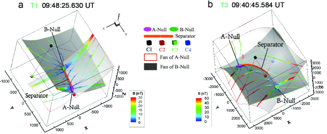
Figure 25: (a) Reconstruction of (a) an antiparallel reconnection region and (b) a component reconnection region. (From Guo et al. [142] with permission.)

Observations in the magnetotail also show that separator reconnection can demonstrate features of both antiparallel and component reconnection. Fig. 25 shows the reconstructed magnetic structures for both cases [142]. Radial null pairs and the separator lines are present. For component reconnection, the separator is long, and the four Cluster spacecraft cross the central part of the separator line, where the magnetic strength is more than 10 nT by comparison with the ambient field strength of 20 – 30 nT. The large magnetic strength implies a large guide field. For antiparallel reconnection, the two nulls are close to the spacecraft tetrahedron and the maximum field strength along the separator is only several nTs, which gives a small guide field.

3.3 Quasi-Separator Reconnection: Modelling and Observations

Because of the strong distortion of the magnetic field line mapping at QSLs, strong currents tend to build up at quasi-separators, which, when no nulls or separators are present, are therefore preferential locations for reconnection in general 3D systems[16, 17]. Thus, in order to study quasi-separator reconnection, it is important first to carefully ensure that no nulls or separators are present. QSL locations are found by measuring the squashing degree Q [18], which does not distinguish between separators and quasi-separators. The role of quasi-separator reconnection in eruptive and confined flares has been widely investigated in numerical simulations and observations. In the analytical work of Démoulin et al.[143], QSLs tend to wrap around flux ropes and delineate the frontier between different classes of field line (Fig.26). The intersection of QSLs with the lower boundary gives a shape that is typical of observed flare ribbons[144].

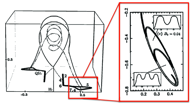
Figure 26: QSL footprints associated with a flux rope and a zoom of the hook-shaped part. Dash-dotted field lines denote the central part of the twisted flux rope and solid curves the field lines at the periphery of the flux rope. Dotted curves show the small arcade lying underneath the flux rope. The QSL footprints form two elongated strips on both sides of the inversion line. The footpoints of the twisted flux rope are located inside the hook-shaped part of QSL footprints. (From Démoulin et al.[143] with permission.)

After the notion of QSLs was proposed by Priest and Démoulin [16], comparison of QSL locations in flaring ARs with flare brightenings was carried out by Démoulin and colleagues and others, using a linear force-free extrapolation [145, 146] or a nonlinear one [147, 148]. The photospheric traces of QSLs often match well the locations of H$\alpha$ flare ribbons (often double J-shaped), while the 3D structure of QSLs and current concentrations resemble an S-shaped sigmoid and outline a flux rope.

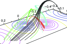
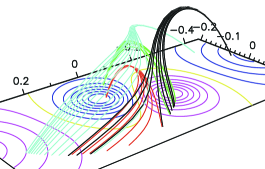
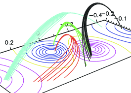
Figure 27: Evolution of flipping or slipping field lines in a numerical simulation. Pink (blue) contours stand for positive (negative) polarity magnetic fields. Four sets of magnetic field lines (red, black, cyan and green lines) are integrated from fixed footpoints and their conjugate footpoints gradually flip or slip along arc-shaped trajectories. (From Aulanier et al.[68] with permission.)

Flipping or slipping of field lines takes place in all 3D reconnection models. It has been demonstrated clearly in 3D resistive simulations on quasi-separator reconnection by Aulanier et al.[68] in Fig.27. Reconnection naturally occurs along arc-shaped QSLs and causes red field lines to reconnect with black ones through field line slippage. Ultimately, the initial red field lines connecting the inner bipole and black field lines connecting the outer bipole evolve into new lateral red and black field lines. A similar process occurs between cyan and green field lines.

Figure 28: Panel (a) shows a A cartoon for a 3D standard model of eruptive flares. The grey area indicates the QSL volume and a current layer wrapping around a torus-unstable flux rope. The blue and yellow loops form the outer envelope of the flux rope, and the green and orange lines indicate the newly formed flare loops due to the occurrence of reconnection. (From Janvier et al.[149] with permission.) Panel (b) displays the isosurface of vertical current sheet that is formed underlying the erupting flux rope. (From Kliem et al.[150] with permission.) Panel (c) shows a 2D vertical cut of the electric current under the rising flux rope, presenting a cusp shape. (From Janvier et al.[151]. Reproduced with permission from Astronomy & Astrophysics.)

Janvier et al.[151] have simulated an eruptive flare caused by a torus-unstable flux rope. They found a linear correlation between the slippage speed and strength of the QSL. Based on 3D MHD simulations and observations, Aulanier, Kliem and colleagues [152, 149] proposed 3D extensions to the standard 2D CSHKP flare model (Fig.28a). As the flux rope expands, regions of high current density are formed along separatrices or QSLs (the grey areas in Fig.28a), and the footprints of the current layers give double J-shaped flare ribbons. Reconnection within the current layers causes apparent slippage of flare ribbons, together with a cusp-shaped region of high current density (Fig.28c), reminiscent of an HFT (Sec.22.2) [147, 148].

In the past 10 years, rich observations of flare loops and footpoints have become available with high time and spatial resolution. Aulanier et al.[153] reported fast bidirectional slippage of coronal loops. SDO flare observations have revealed many features of both 3D separator and quasi-separator reconnection. Dudík et al.[154] reported slipping motions of both the flare and erupting loops along developing flare ribbons at speeds of tens of km s^-1.

Combining imaging and spectroscopic observations from SDO and IRIS, Li & Zhang[155] found quasi-periodic patterns with a period of 3-6 minutes in small-scale bright knots that moved along flare ribbons, while the flare loops exhibited quasi-periodic slippage along the flare ribbon at a speed of 20-110 km s^-1 (Fig.29).

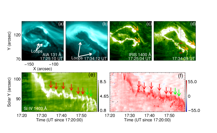
Figure 29: Panels (a)-(d) show slipping hot flare loops and flare ribbons as seen in SDO/AIA 131 Å and IRIS 1400 Å. The arrows in panels (c)-(d) denote the slipping direction of flare ribbons. Panels (e)-(f) display the temporal evolution of peak intensity and Doppler shift in the spatial range indicated by the two red horizontal bars in panel (d). These parameters are obtained by applying single-Gaussian fits to the Si IV 1402.77 Å line. The arrows in panels (e)-(f) point to the peaks of wave-like evolution and correspond to the times when the slipping knots pass by the location of the IRIS slit. (From Li & Zhang[155] with permission.)

Both separator and quasi-separator flare models suggest bi-directional slippage along flare ribbons, with one direction toward the ribbon hook building up the erupting flux rope and the opposite direction producing slippage of flare loops. Dudík et al.[156] observed flare loops slipping in opposite directions at speeds of 20-40 km s^-1, but occasionally even faster velocities of 400-450 km s^-1 have been found [157]. Also, Jing et al.[158] observed a long-duration flare ribbon slippage at a QSL footprint across a long distance ($\sim$60 Mm).

During eruptive flares, 3D reconnection geometries are more complex than in 2D. The photospheric footpoints, for example, are observed to brighten sequentially along the polarity inversion line during the rise phase [159, 160, 161], as modelled by Priest and Longcope [139] in terms of zipper reconnection (Sec.33.2). Also, Li et al.[159] finds one end of an eruptive flux rope is fixed and the other end exhibits apparent slippage along a hook-shaped flare ribbon. Aulanier & Dudík[161] have proposed that a series of reconnections between the flux-rope field lines and its surrounding arcade within QSLs can produce a gradual drifting of flux rope footpoints.

Moreover, both separator and quasi-separator reconnection have been shown to play a role in confined solar flares[162, 163]. Li et al.[162] found bi-directional slippage of ribbon substructures along a ribbon in a confined flare. In fact, some confined flares are characterized by slippage and a stable filament, whereas others possess a failed eruption of a filament or flux rope[163]. Just as for separators, quasi-separators may also play an important role in coronal heating[164, 165]. A study by Schrijver et al.[165] compared bright loops fanning out from ARs with topological features of QSLs, suggesting magnetic energy release at separator or quasi-separator current sheets. Mandrini et al.[166] found that persistent plasma upflows at the edge of ARs are often located near QSLs, and suggested that reconnection causes plasma to flow from the high-pressure AR loops to neighboring large-scale low-pressure loops in the quiet Sun.

4 Conclusion

Null points have been shown to be present in abundance in the solar corona due to the complexity of magnetic flux concentrated by photospheric convective motions and projecting through the solar surface into the atmosphere. The same is highly likely to be true in other astrophysical environments such as the coronae of other stars and of accretion disks, and nulls are also present in planetary magnetospheres.

The fans of null points form a rich skeleton of separatrix surfaces threading the corona, which intersect in separator field lines. The dominant forms of magnetic reconnection, driven by photospheric motions (in solar coronal heating) or magnetohydrodynamic instability or nonequilibrium (in solar flares), are therefore likely to be null reconnection or separator reconnection (and their “quasi" equivalents).

During null or separator reconnection, the magnetic field lines rapidly flip or slip through the plasma, while, at a null point or separatrix, there is a discontinuity in the mapping of magnetic field lines. Moreover, the behaviour is very similar at surfaces called QSLs, where the mapping gradient of field lines is very large but not singular, or in a region that one may call a quasi-null, where the magnetic field becomes small but non-zero. Such QSLs intersect in quasi-separators or HFTs.

Nulls, separatrices and separators are purely topological features, but, when the appropriate plasma flows are present, they are prime locations for the build-up of electric currents and therefore of magnetic reconnection in diffusion regions. Although quasi-nulls, QSLs and quasi-separators are not topological features, since there is no change of topology at them, they are important geometrical features of a complex magnetic configuration. They often represent the remnants of nulls, separatrices and separators when a weak magnetic field is superposed to smooth away the null points.

However, just like their topological cousins, provided appropriate plasma flows are present, currents will also build up near quasi-nulls and quasi-separators, and so reconnection will take place at them. Indeed, quasi-separator reconnection is also thought to be important in solar coronal heating and solar flares, but physically there is very little difference between it and separator reconnection. The reason for the close similarity is simply that, whereas reconnection takes place in strict 2D precisely at a null point within a diffusion region, in 3D QSL reconnection or in 3D null-point or separator reconnection the field lines continuously change their connections everywhere throughout the diffusion region that surrounds the null or separator.

Three-dimensional reconnection is a complex nonlinear process. However, its basic theory (Sec.2) has now been complemented by sophisticated numerical experiments that can go beyond the simplifying assumptions of theory and produce more realistic modelling of the process (Sec.3). In addition, over recent years a new generation of solar telescopes has produced remarkable observations that have validated the basic theory and revealed a wealth of detail on null, separator and quasi-separator reconnection in action. These include the location of current concentrations and the sites of energy release, the presence of flipping or slipping of field lines, and the creation of jets, both in coronal heating events and in solar flares.

For solar atmospheric heating, reconnection is likely to provide a major contribution, especially low down in the atmosphere and in active regions. In particular, the flux tube tectonics model is a modern updating of the traditional nanoflare model, and a promising new development inspired by ultra-high resolution magnetograms is the flux cancellation model for both chromospheric and coronal heating.

For solar flares, we would like to propose the following new 3D paradigm, which brings together a wide range of properties that have been studied separately. The first two are taken over from the standard 2D paradigm, while properties (iv,v,vii) arise from studies of separator reconnection [66, 136, 138, 139, 140] and properties (viii,ix) from quasi-separator reconnection [159, 149, 20], but they apply equally to both separator and quasi-separator reconnection.

(i) A magnetic flux rope erupts due to magnetic nonequilibrium or instability and forms a vertical current sheet below the rope;

(ii) Reconnection in the current sheet creates a rising arcade of flare loops with separating chromospheric ribbons at their feet as the height of the reconnection location increases;

(iii) At low spatial and temporal resolution, reconnection may appear to be quasi-steady and laminar, especially during the late stages of a flare, but, at high resolution, especially during the impulsive phase, it is often impulsive and bursty in time and fragmented in space, as revealed even during the main phase by observed supra-arcade downflows [167, 168];

(iv) Reconnection starts at one location in the current sheet and creates two kernels of chromospheric emission; then, during the rise phase, it spreads along the sheet above the polarity inversion line, gradually energizing the whole coronal arcade and forming the flare ribbons by zipper reconnection [139]; the ribbons then move apart during the main phase;

(v) Some of the twist in an erupting flux rope was present before the eruption, but most of it is created during the process of reconnection by the conversion of mutual magnetic helicity into self-helicity [140];

(vi) The two main types of reconnection occurring in flares are null-point reconnection, which forms flare ribbons that are roughly circular, and separator (or quasi-separator) reconnection, whose ribbons are often straight or S-shaped;

(vii) The topology (or quasi-topology) of an active region can be highly complex and partitioned into many domains bounded by separatrix (or quasi-separatrix) surfaces. Reconnection between different domains occurs at separators (or quasi-separators) and allows the energy release to spread from one domain to another, with the flare ribbons following a sequence of spines (or quasi-spines) [66]; in the same way, a series of coronal eruptions may be explained as a series of separator (or quasi-separator) reconnections between one region and another [138];

(viii) Flare ribbons often have hook-like ends [159], which are the ends of flux ropes bounded by quasi-separatrix (or separatrix) surfaces [149];

(ix) Flipping or slipping of magnetic fields, which was predicted to be a property of all 3D reconnection models, is observed in the behaviour of flare loops and their footpoints [20].

In the Earth’s magnetosphere, observations with four spacecrafts can better identify the presence of null points and separators and can directly obtain magnetic and plasma properties around them. Spiral null points occur more frequently than radial null points. The former can serve as the skeleton of magnetic flux ropes and play an important role in magnetic energy release and plasma acceleration in the 3D reconnection region. At the reconnection site, separator reconnection can demonstrate features of both antiparallel reconnection and component reconnection. Additionally, the formation and evolution of clusters of null points are related to magnetic turbulence and significant energy dissipation.

It is clear that in future, developments in the basic theory, numerical simulations and high-resolution observations will continue to complement one another and to spur each other on to a fuller understanding. It is also clear that the main distinction in types of reconnection is between null-point reconnection and separator reconnection, and that the distinction between separator and quasi-separator reconnection is a largely theoretical distinction that is unimportant for the physical consequences and observations of energy release. Furthermore, likely future developments concern unsteady patchy reconnection and better links between a macroscopic MHD understanding and a microscopic collisionless understanding.

There are no ethics issues. This article has no additional data.

All the authors have contributed equally to all sections.

There are no competing interests.

This research is supported by the Strategic Priority Research Program of Chinese Academy of Sciences (XDB41000000), the National Natural Science Foundations of China (11773039, 11903050, 11790304, 11790300 and 41704169), the National Key R&D Program of China (2019YFA0405000), Key Programs of the Chinese Academy of Sciences (QYZDJ-SSW-SLH050), the Youth Innovation Promotion Association of CAS (2017078) and NAOC Nebula Talents Program. R.L.G. is supported by the Incoming Post-Docs in Sciences, Technology, Engineering, Materials and Agrobiotechnology (IPD-STEMA) project from Université de Liège.

E.P. is grateful to Guillaume Aulanier, Pascal Démoulin, Terry Forbes, Gunnar Hornig, Dana Longcope, Clare Parnell, David Pontin and Slava Titov for teaching him so much about the intriguing nature of reconnection.

The ideas presented here represent our own ideas together with our understanding of those of other researchers.

References

- [1] Pontin DI. 2012 Theory of magnetic reconnection in solar and astrophysical plasmas. Philosophical Transactions of the Royal Society of London Series A 370, 3169–3192.
- [2] Longcope DW, Tarr LA. 2015 Relating magnetic reconnection to coronal heating. Phil. Trans. Roy. Soc. Lond. Series A 373, 40263.
- [3] Janvier M. 2017 Three-dimensional magnetic reconnection and its application to solar flares. Journal of Plasma Physics 83, 535830101.
- [4] Dungey JW. 1953 The motion of magnetic fields. Mon. Not. R. Astron. Soc. 113, 679.
- [5] Parker EN. 1957 Sweet’s Mechanism for Merging Magnetic Fields in Conducting Fluids. J. Geophys. Res. 62, 509–520.
- [6] Sweet PA. 1958 The Neutral Point Theory of Solar Flares. In Lehnert B, editor, Electromagnetic Phenomena in Cosmical Physics vol. 6IAU Symposium p. 123.
- [7] Petschek H. 1964 Magnetic field annihilation. In The Physics of Solar Flares pp. 425–439. Washington: NASA Spec. Publ. SP-50.
- [8] Priest E, Forbes T. 1986 New models for fast, steady-state reconnection. J. Geophys. Res. 91, 5579–5588.
- [9] Priest E, Forbes T. 2000 Magnetic Reconnection: MHD Theory and Applications. Cambridge, UK: Cambridge University Press.
- [10] Ni L, Ji H, Murphy NA, Jara-Almonte J. 2020 Magnetic reconnection in partially ionized plasmas. Proceedings of the Royal Society of London Series A 476, 90867.
- [11] Schindler K, Hesse M, Birn J. 1988 General magnetic reconnection, parallel electric fields, and helicity. Journal of Geophysical Research 93, 5547–5557.
- [12] Hesse M, Schindler K. 1988 A theoretical foundation of general magnetic reconnection. Journal of Geophysical Research 93, 5559–5567.
- [13] Priest ER, Hornig G, Pontin DI. 2003 On the nature of three-dimensional magnetic reconnection. Journal of Geophysical Research (Space Physics) 108, 1285.
- [14] Lau YT, Finn JM. 1990 Three-dimensional Kinematic Reconnection in the Presence of Field Nulls and Closed Field Lines. Astrophysical Journal 350, 672.
- [15] Sweet P. 1958 The production of high energy particles in solar flares. Nuovo Cimento Suppl. 8, 188–196.
- [16] Priest ER, Démoulin P. 1995 Three-dimensional magnetic reconnection without null points. 1. Basic theory of magnetic flipping. Journal of Geophysical Research 100, 23443–23464.
- [17] Demoulin P, Henoux JC, Priest ER, Mandrini CH. 1996 Quasi-Separatrix layers in solar flares. I. Method.. Astronomy and Astrophysics 308, 643–655.
- [18] Titov VS, Hornig G, Démoulin P. 2002 Theory of magnetic connectivity in the solar corona. Journal of Geophysical Research (Space Physics) 107, 1164.
- [19] Priest ER, Forbes TG. 1992 Magnetic Flipping: Reconnection in Three Dimensions Without Null Points. Journal of Geophysical Research 97, 1521–1531.
- [20] Mandrini CH, Demoulin P, Henoux JC, Machado ME. 1991 Evidence for the interaction of large scale magnetic structures in solar flares.. Astronomy and Astrophysics 250, 541–547.
- [21] Shibata K, Magara T. 2011 Solar Flares: Magnetohydrodynamic Processes. Living Reviews in Solar Physics 8, 6.
- [22] Yokoyama T, Akita K, Morimoto T, Inoue K, Newmark J. 2001 Clear Evidence of Reconnection Inflow of a Solar Flare. Astrophysical Journal Letters 546, L69–L72.
- [23] Savage SL, McKenzie DE, Reeves KK, Forbes TG, Longcope DW. 2010 Reconnection Outflows and Current Sheet Observed with Hinode/XRT in the 2008 April 9 “Cartwheel CME” Flare. Astrophysical Journal 722, 329–342.
- [24] Sun JQ, Cheng X, Ding MD, Guo Y, Priest ER, Parnell CE, Edwards SJ, Zhang J, Chen PF, Fang C. 2015 Extreme ultraviolet imaging of three-dimensional magnetic reconnection in a solar eruption. Nature Communications 6, 7598.
- [25] McKenzie DE, Hudson HS. 1999 X-Ray Observations of Motions and Structure above a Solar Flare Arcade. Astrophysical Journal Letters 519, L93–L96.
- [26] Li LP, Zhang J, Su JT, Liu Y. 2016 Oscillation of Current Sheets in the Wake of a Flux Rope Eruption Observed by the Solar Dynamics Observatory. The Astrophysical Journal Letters 829, L33.
- [27] Masuda S, Kosugi T, Hara H, Tsuneta S, Ogawara Y. 1994 A loop-top hard X-ray source in a compact solar flare as evidence for magnetic reconnection. Nature 371, 495–497.
- [28] Lin J, Ko YK, Sui L, Raymond JC, Stenborg GA, Jiang Y, Zhao S, Mancuso S. 2005 Direct Observations of the Magnetic Reconnection Site of an Eruption on 2003 November 18. Astrophysical Journal 622, 1251–1264.
- [29] Xue Z, Yan X, Yang L, Wang J, Feng S, Li Q, Ji K, Zhao L. 2018 Spectral and Imaging Observations of a Current Sheet Region in a Small-scale Magnetic Reconnection Event. Astrophysical Journal Letters 858, L4.
- [30] Su Y, Veronig AM, Holman GD, Dennis BR, Wang T, Temmer M, Gan W. 2013 Imaging coronal magnetic-field reconnection in a solar flare. Nature Physics 9, 489–493.
- [31] Kopp RA, Pneuman GW. 1976 Magnetic reconnection in the corona and the loop prominence phenomenon.. Solar Physics 50, 85–98.
- [32] Priest ER, Forbes TG. 1990 Magnetic field evolution during prominence eruptions and two-ribbon flares. Solar Phys. 126, 319–350.
- [33] Kliem B, Török T. 2006 Torus Instability. Physical Review Letters 96, 255002.
- [34] Priest ER. 2014 Magnetohydrodynamics of the Sun. Cambridge, UK: Cambridge University Press.
- [35] Baty H, Forbes TG, Priest ER. 2014 The formation and stability of Petschek reconnection. Physics of Plasmas 21, 112111.
- [36] Priest E. 1986 Magnetic reconnection on the Sun. Mit. Astron. Ges. 65, 41–51.
- [37] Forbes T, Priest E. 1987 A comparison of analytical and numerical models for steadily-driven magnetic reconnection. Rev. Geophys. 25, 1583–1607.
- [38] Loureiro NF, Schekochihin AA, Cowley SC. 2007 Instability of current sheets and formation of plasmoid chains. Phys. Plasmas 14, 100703.
- [39] Bhattacharjee A, Huang YM, Yang H, Rogers B. 2009 Fast reconnection in high-Lundquist-number plasmas due to the plasmoid instability. Phys. Plasmas 16, 112102.
- [40] Shay MA, Drake JF, Denton RE, Biskamp D. 1998 Structure of the dissipation region during collisionless magnetic reconnection. J. Geophys. Res. 103, 9165–9176.
- [41] Priest ER, Titov VS. 1996 Magnetic Reconnection at Three-Dimensional Null Points. Proceedings of the Royal Society of London Series A 354, 2951–2992.
- [42] Parnell CE, Smith JM, Neukirch T, Priest ER. 1996 The structure of three-dimensional magnetic neutral points. Physics of Plasmas 3, 759–770.
- [43] Edwards SJ, Parnell CE. 2015 Null Point Distribution in Global Coronal Potential Field Extrapolations. Solar Phys. 290, 2055–2076.
- [44] Titov VS, Priest ER, Démoulin P. 1993 Conditions for the appearance of bald patches at the solar surface. Astron. Astrophys. 276, 564–570.
- [45] Longcope DW, Cowley SC. 1996 Current sheet formation along three-dimensional magnetic separators. Physics of Plasmas 3, 2885–2897.
- [46] Parnell CE, Haynes AL, Galsgaard K. 2010a Structure of magnetic separators and separator reconnection. J. Geophys. Res. 115, 2102.
- [47] Haynes A, Parnell C, Galsgaard K, Priest E. 2007 Magnetohydrodynamic evolution of magnetic skeletons. Proc. Roy. Soc. Lond. 463, 1097–1115.
- [48] Priest E, Démoulin P. 1995 3D reconnection without null points. J. Geophys. Res. 100, 23443–23463.
- [49] Parnell CE, Maclean RC, Haynes AL. 2010b The Detection of Numerous Magnetic Separators in a Three-Dimensional Magnetohydrodynamic Model of Solar Emerging Flux. Astrophys. J. Letts. 725, L214–L218.
- [50] Woltjer L. 1958 A theorem on force-free fields. Proc. Nat. AcaD.S.i. USA 44, 489.
- [51] Heyvaerts J, Priest E. 1984 Coronal heating by reconnection in DC current systems - A theory based on Taylor’s hypothesis. Astron. Astrophys. 137, 63–78.
- [52] Berger M, Field G. 1984 The topological properties of magnetic helicity. J. Fluid Mech. 147, 133–148.
- [53] Berger MA. 1988 An energy formula for nonlinear force-free magnetic fields. Astron. Astrophys. 201, 355–361.
- [54] Yeates AR, Hornig G. 2013 Unique topological characterization of braided magnetic fields. Phys. Plasmas 20, 012102.
- [55] Yeates AR, Hornig G. 2016 The global distribution of magnetic helicity in the solar corona. Astronomy & Astrophysics 594, A98.
- [56] Hornig G, Schindler K. 1996 Magnetic topology and the problem of its invariant definition. Phys. Plasmas 3, 781–791.
- [57] Priest ER, Pontin DI. 2009 Three-dimensional null point reconnection regimes. Physics of Plasmas 16, 122101–122101.
- [58] Hornig G, Priest ER. 2003 Evolution of magnetic flux in an isolated reconnection process. Phys. Plasmas 10, 2712–2721.
- [59] Pontin DI, Galsgaard K. 2007 Current amplification and magnetic reconnection at a three-dimensional null point: physical characteristics. J. Geophys. Res. 112, A03103.
- [60] Pontin DI, Hornig G, Priest ER. 2005 Kinematic reconnection at a magnetic null point: fan-aligned current. Geophysical and Astrophysical Fluid Dynamics 99, 77–93.
- [61] Galsgaard K, Priest ER, Nordlund Å. 2000 Three-dimensional Separator Reconnection - How Does It Occur?. Solar Phys. 193, 1–16.
- [62] Restante AL, Aulanier G, Parnell CE. 2009 How skeletons turn into quasi-separatrix layers in source models. Astron. Astrophys. 508, 433–443.
- [63] Parnell CE, Haynes AL, Galsgaard K. 2008 Recursive reconnection and magnetic skeletons. Astrophys. J. 675, 1656–1667.
- [64] Longcope DW. 2001 Separator current sheets: generic features in minimum-energy magnetic fields subject to flux constraints. Phys. Plasmas 8, 5277–5289.
- [65] Longcope DW. 1998 A model for current sheets and reconnection in X-ray bright points. Astrophys. J. 507, 433–442.
- [66] Longcope DW, Beveridge C. 2007 A Quantitative, Topological Model of Reconnection and Flux Rope Formation in a Two-Ribbon Flare. Astrophys. J. 669, 621–635.
- [67] Priest ER, Syntelis P. 2021 Chromospheric and coronal heating and jet acceleration due to reconnection driven by flux cancellation. I. At a three-dimensional current sheet. Astron. and Astrophys. 647, A31.
- [68] Aulanier G, Pariat E, Démoulin P, DeVore CR. 2006 Slip-Running Reconnection in Quasi-Separatrix Layers. Solar Physics 238, 347–376.
- [69] Titov VS, Galsgaard K, Neukirch T. 2003 Magnetic pinching of hyperbolic flux tubes. I. Basic estimations. Astrophys. J. 582, 1172–1189.
- [70] Aulanier G, Pariat E, Démoulin P. 2005 Current-sheet formation in quasi-separatrix layers and hyperbolic flux tubes. Astron. & Astrophys. 444, 961–976.
- [71] Xiao CJ, Wang XG, Pu ZY, Zhao H, Wang JX, Ma ZW, Fu SY, Kivelson MG, Liu ZX, Zong QG, Glassmeier KH, Balogh A, Korth A, Reme H, Escoubet CP. 2006 In situ evidence for the structure of the magnetic null in a 3D reconnection event in the Earth’s magnetotail. Nature Physics 2, 478–483.
- [72] Guo R, Pu Z, Xiao C, Wang X, Fu S, Xie L, Zong Q, He J, Yao Z, Zhong J, Li J. 2013 Separator reconnection with antiparallel/component features observed in magnetotail plasmas. Journal of Geophysical Research (Space Physics) 118, 6116–6126.
- [73] Dorelli JC, Bhattacharjee A, Raeder J. 2007 Separator reconnection at Earth’s dayside magnetopause under generic northward interplanetary magnetic field conditions. Journal of Geophysical Research (Space Physics) 112, A02202.
- [74] Longcope DW. 1996 Topology and Current Ribbons: A Model for Current, Reconnection and Flaring in a Complex, Evolving Corona. Solar Physics 169, 91–121.
- [75] Lynch BJ, Antiochos SK, DeVore CR, Luhmann JG, Zurbuchen TH. 2008 Topological Evolution of a Fast Magnetic Breakout CME in Three Dimensions. Astrophysical Journal 683, 1192–1206.
- [76] Raouafi NE, Patsourakos S, Pariat E, Young PR, Sterling AC, Savcheva A, Shimojo M, Moreno-Insertis F, DeVore CR, Archontis V, Török T, Mason H, Curdt W, Meyer K, Dalmasse K, Matsui Y. 2016 Solar Coronal Jets: Observations, Theory, and Modeling. Space Science Reviews 201, 1–53.
- [77] Shen Y. 2021 Observation and modelling of solar jets. Proceedings of the Royal Society of London Series A 477, 217.
- [78] Török T, Aulanier G, Schmieder B, Reeves KK, Golub L. 2009 Fan-Spine Topology Formation Through Two-Step Reconnection Driven by Twisted Flux Emergence. Astrophysical Journal 704, 485–495.
- [79] Liu W, Berger TE, Title AM, Tarbell TD, Low BC. 2011 Chromospheric Jet and Growing “Loop” Observed by Hinode: New Evidence of Fan-spine Magnetic Topology Resulting from Flux Emergence. Astrophysical Journal 728, 103.
- [80] Pontin DI, Priest ER, Galsgaard K. 2013 On the Nature of Reconnection at a Solar Coronal Null Point above a Separatrix Dome. Astrophysical Journal 774, 154.
- [81] Masson S, Pariat E, Aulanier G, Schrijver CJ. 2009 The Nature of Flare Ribbons in Coronal Null-Point Topology. Astrophysical Journal 700, 559–578.
- [82] Yang S, Zhang Q, Xu Z, Zhang J, Zhong Z, Guo Y. 2020 Imaging and Spectral Study on the Null Point of a Fan-spine Structure During a Solar Flare. Astrophysical Journal 898, 101.
- [83] Hou Y, Li T, Yang S, Zhang J. 2019 A Secondary Fan-spine Magnetic Structure in Active Region 11897. Astrophysical Journal 871, 4.
- [84] Wang H, Liu C. 2012 Circular Ribbon Flares and Homologous Jets. Astrophysical Journal 760, 101.
- [85] Song YL, Guo Y, Tian H, Zhu XS, Zhang M, Zhu YJ. 2018 Observations of a White-light Flare Associated with a Filament Eruption. Astrophysical Journal 854, 64.
- [86] Hood AW, Priest ER. 1981 Critical conditions for magnetic instabilities in force-free coronal loops. Geophysical and Astrophysical Fluid Dynamics 17, 297–318.
- [87] Sun X, Hoeksema JT, Liu Y, Aulanier G, Su Y, Hannah IG, Hock RA. 2013 Hot Spine Loops and the Nature of a Late-phase Solar Flare. Astrophysical Journal 778, 139.
- [88] Zhang QM, Li D, Ning ZJ, Su YN, Ji HS, Guo Y. 2016 Explosive Chromospheric Evaporation in a Circular-ribbon Flare. Astrophysical Journal 827, 27.
- [89] Moore RL, Cirtain JW, Sterling AC, Falconer DA. 2010 Dichotomy of Solar Coronal Jets: Standard Jets and Blowout Jets. Astrophysical Journal 720, 757–770.
- [90] Yang K, Guo Y, Ding MD. 2015 On the 2012 October 23 Circular Ribbon Flare: Emission Features and Magnetic Topology. Astrophysical Journal 806, 171.
- [91] Li T, Yang S, Zhang Q, Hou Y, Zhang J. 2018 Two Episodes of Magnetic Reconnections during a Confined Circular-ribbon Flare. Astrophysical Journal 859, 122.
- [92] Pontin D, Galsgaard K, Démoulin P. 2016 Why Are Flare Ribbons Associated with the Spines of Magnetic Null Points Generically Elongated?. Solar Physics 291, 1739–1759.
- [93] Antiochos SK, DeVore CR, Klimchuk JA. 1999 A Model for Solar Coronal Mass Ejections. Astrophysical Journal 510, 485–493.
- [94] Wyper PF, Antiochos SK, DeVore CR. 2017 A universal model for solar eruptions. Nature 544, 452–455.
- [95] Xiao CJ, Wang XG, Pu ZY, Zhao H, Wang JX, Ma ZW, Fu SY, Kivelson MG, Liu ZX, Zong QG, Glassmeier KH, Balogh A, Korth A, Reme H, Escoubet CP. 2006 In situ evidence for the structure of the magnetic null in a 3D reconnection event in the Earth’s magnetotail. Nature Physics 2, 478–483.
- [96] He JS, Tu CY, Tian H, Xiao CJ, Wang XG, Pu ZY, Ma ZW, Dunlop MW, Zhao H, Zhou GP, Wang JX, Fu SY, Liu ZX, Zong QG, Glassmeier KH, Reme H, Dandouras I, Escoubet CP. 2008 A magnetic null geometry reconstructed from Cluster spacecraft observations. Journal of Geophysical Research (Space Physics) 113, A05205.
- [97] Deng XH, Zhou M, Li SY, Baumjohann W, Andre M, Cornilleau N, Santolík O, Pontin DI, Reme H, Lucek E, Fazakerley AN, Decreau P, Daly P, Nakamura R, Tang RX, Hu YH, Pang Y, Büchner J, Zhao H, Vaivads A, Pickett JS, Ng CS, Lin X, Fu S, Yuan ZG, Su ZW, Wang JF. 2009 Dynamics and waves near multiple magnetic null points in reconnection diffusion region. Journal of Geophysical Research: Space Physics 114.
- [98] Xiao CJ, Wang XG, Pu ZY, Ma ZW, Zhao H, Zhou GP, Wang JX, Kivelson MG, Fu SY, Liu ZX, Zong QG, Dunlop MW, Glassmeier KH, Lucek E, Reme H, Dandouras I, Escoubet CP. 2007 Satellite observations of separator-line geometry of three-dimensional magnetic reconnection. Nature Physics 3, 609–613.
- [99] Dunlop MW, Zhang QH, Xiao CJ, He JS, Pu Z, Fear RC, Shen C, Escoubet CP. 2009 Reconnection at high latitudes: antiparallel merging. Phys Rev Lett 102, 075005.
- [100] Wendel DE, Adrian ML. 2013 Current structure and nonideal behavior at magnetic null points in the turbulent magnetosheath. Journal of Geophysical Research: Space Physics 118, 1571–1588.
- [101] Chen ZZ, Fu HS, Wang Z, Liu CM, Xu Y. 2019 Evidence of Magnetic Nulls in the Reconnection at Bow Shock. Geophysical Research Letters 46, 10209–10218.
- [102] He JS, Zong QG, Deng XH, Tu CY, Xiao CJ, Wang XG, Ma ZW, Pu ZY, Lucek E, Pedersen A, Fazakerley A, Cornilleau-Wehrlin N, Dunlop MW, Tian H, Yao S, Tan B, Fu SY, Glassmeier KH, Reme H, Dandouras I, Escoubet CP. 2008 Electron trapping around a magnetic null. Geophysical Research Letters 35, L14104.
- [103] Eriksson E, Vaivads A, Khotyaintsev YV, Khotyayintsev VM, André M. 2015 Statistics and accuracy of magnetic null identification in multispacecraft data. Geophysical Research Letters 42, 6883–6889.
- [104] Olshevsky V, Deca J, Divin A, Peng IB, Markidis S, Innocenti ME, Cazzola E, Lapenta G. 2016 Magnetic Null Points in Kinetic Simulations of Space Plasmas. Astrophysical Journal 819, 52.
- [105] Guo R, Pu Z, Chen LJ, Fu S, Xie L, Wang X, Dunlop M, Bogdanova YV, Yao Z, Xiao C, He J, Fazakerley AN. 2016 In-situ observations of flux ropes formed in association with a pair of spiral nulls in magnetotail plasmas. Physics of Plasmas 23, 052901.
- [106] Guo R, Pu Z, Yao Z, Dunlop M, Bogdanova YV, Wei Y, Wang X, Xiao C, He J, Fu S, Xie L, Fazakerley AN, Wan W. 2019 A three-dimensional model of spiral null pair to form ion-scale flux ropes in magnetic reconnection region observed by Cluster. Physics of Plasmas 26, 112901.
- [107] Zhao H, Wang JX, Zhang J, Xiao CJ, Wang HM. 2008 Determination of the topology skeleton of magnetic fields in a solar active region. Chinese Journal of Astronomy and Astrophysics 8, 133–145.
- [108] Chen LJ, Bhattacharjee A, Puhl-Quinn PA, Yang H, Bessho N, Imada S, Mühlbachler S, Daly PW, Lefebvre B, Khotyaintsev Y, Vaivads A, Fazakerley A, Georgescu E. 2007 Observation of energetic electrons within magnetic islands. Nature Physics 4, 19–23.
- [109] Fu HS, Vaivads A, Khotyaintsev YV, André M, Cao JB, Olshevsky V, Eastwood JP, Retinò A. 2017 Intermittent energy dissipation by turbulent reconnection. Geophysical Research Letters 44, 37–43.
- [110] Guo R, Pu Z, Fu S, Xie L, Dunlop M, Bogdanova YV, He J, Wang X, Yao Z. 2016 Evolution of clustered magnetic nulls in a turbulent-like reconnection region in the magnetotail. Science Bulletin 61, 1145–1150.
- [111] Greene JM. 1988 Geometrical properties of three-dimensional reconnecting magnetic fields with nulls. Journal of Geophysical Research 93, 8583–8590.
- [112] Murphy NA, Parnell CE, Haynes AL. 2015 The appearance, motion, and disappearance of three-dimensional magnetic null points. Physics of Plasmas 22, 102117.
- [113] Priest E, Lonie D, Titov V. 1996 Bifurcations of magnetic topology by the creation or annihilation of null points. J. Plasma Phys. 56, 507–530.
- [114] Longcope DW. 2005 Topological methods for the analysis of solar magnetic fields. Liv. Rev. in Solar Phys. 2, 1–72.
- [115] Titov VS. 2007 Generalized Squashing Factors for Covariant Description of Magnetic Connectivity in the Solar Corona. Astrophysical Journal 660, 863–873.
- [116] Titov V, Forbes T, Priest E, Mikić Z, Linker J. 2009 Slip-squashing factors as a measure of three-dimensional magnetic reconnection. Astrophys. J. 693, 1029–1044.
- [117] Parnell CE, Haynes AL, Maclean RC. 2011 Three Dimensional Magnetic Reconnection at Null Points and Separators. In Miralles MP, Sánchez Almeida J, editors, The Sun, the Solar Wind, and the Heliosphere vol. 4 p. 147.
- [118] Schrijver CJ, Title AM, Harvey, K. L. anD.S.eeley NR, Wang YM, van den Oord GHJ, Shine RA, Tarbell TD, Hurlburt NE. 1998 Large-scale coronal heating by the small-scale magnetic field of the Sun. Nature 394, 152–154.
- [119] Parnell CE, Stevenson JEH, Threlfall J, Edwards SJ. 2015 Is magnetic topology important for heating the solar atmosphere?. Philosophical Transactions of the Royal Society of London Series A 373, 20140264–20140264.
- [120] Platten SJ, Parnell CE, Haynes AL, Priest ER, Mackay DH. 2014 The solar cycle variation of topological structures in the global solar corona. Astron. Astrophys. 565, A44.
- [121] Parker E. 1972 Topological dissipation and the small-scale fields in turbulent gases. Astrophys. J. 174, 499–510.
- [122] Galsgaard K, Nordlund Å. 1996 The heating and activity of the solar corona: I Boundary shearing of an initially homogeneous magnetic field. J. Geophys. Res. 101, 13445–13460.
- [123] Pontin DI, Wilmot-Smith AL, Hornig G, Galsgaard K. 2011 Dynamics of braided coronal loops. II. Cascade to multiple small-scale reconnection events. Astron. Astrophys. 525, A57.
- [124] Priest E, Heyvaerts J, Title A. 2002 A Flux Tube Tectonics model for solar coronal heating driven by the magnetic carpet. Astrophys. J. 576, 533–551.
- [125] Priest E, Longcope D, Heyvaerts J. 2005 Coronal heating at separators and separatrices. Astrophys. J. 624, 1057–1071.
- [126] De Moortel I, Galsgaard K. 2006 Numerical modelling of 3D reconnection. II. Comparison between rotational and spinning footpoint motions. Astron. Astrophys. 459, 627–639.
- [127] Parnell CE, Galsgaard K. 2004 Elementary Heating Events – Interaction between Two Flux Sources. II. Rates of Flux Reconnection. Astron. & Astrophys. 428, 595–612.
- [128] Parnell C, Haynes A. 2009 Three-dimensional magnetic reconnection. In Magnetic Coupling Between the Interior and Atmosphere of the Sun pp. 261–276. Heidelberg: Springer-Verlag.
- [129] Priest ER, Chitta LP, Syntelis P. 2018 A Cancellation Nanoflare Model for Solar Chromospheric and Coronal Heating. Astrophys. J. 862, L24.
- [130] Solanki SK, Barthol P, Danilovic S, Feller A, Gandorfer A, Hirzberger J, Riethmüller TL, Schüssler M, Bonet JA, Martínez Pillet V, del Toro Iniesta JC, Domingo V, Palacios J, Knölker M, Bello González N, Berkefeld T, Franz M, Schmidt W, Title AM. 2010 SUNRISE: Instrument, Mission, Data, and First Results. Astrophys. J. Letts. 723, L127–L133.
- [131] Smitha HN, Anusha LS, Solanki SK, Riethmüller TL. 2017 Estimation of the Magnetic Flux Emergence Rate in the Quiet Sun from Sunrise Data. Astrophys. J. Suppl. 229, 17.
- [132] Syntelis P, Priest ER. 2020 A Cancellation Nanoflare Model for Solar Chromospheric and Coronal Heating. III. 3D Simulations and Atmospheric Response. Astrophys. J. 891, 52.
- [133] Chitta LP, Peter H, Priest ER, Solanki SK. 2020 Impulsive coronal heating during the interaction of surface magnetic fields in the lower solar atmosphere. Astronomy & Astrophysics 644, A130.
- [134] Longcope D, Beveridge C, Qiu J, Ravindra B, Barnes G, Dasso S. 2007 Modeling and Measuring the Flux Reconnected and Ejected by the Two-Ribbon Flare/CME Event on 7 November 2004. Solar Phys. 244, 45–73.
- [135] Longcope DW, Silva AVR. 1998 A current ribbon model for energy storage and release with application to the flare 1992 Jan. 7. Solar Phys. 179, 349–377.
- [136] Kazachenko MD, Canfield RC, Longcope DW, Qiu J. 2012 Predictions of Energy and Helicity in Four Major Eruptive Solar Flares. Solar Phys. 277, 165–183.
- [137] Priest E, Bungey T, Titov V. 1997 The 3D topology and interaction of complex magnetic flux systems. Geophys. Astrophys. Fluid Dyn. 84, 127–163.
- [138] Titov VS, Mikic Z, Török T, Linker JA, Panasenco O. 2012 2010 August 1–2 Sympathetic Eruptions. I. Magnetic Topology of the Source-surface Background Field. Astrophys. J. 759, 70.
- [139] Priest ER, Longcope DW. 2017 Flux-Rope Twist in Eruptive Flares and CMEs: Due to Zipper and Main-Phase Reconnection. Solar Phys. 292, 25.
- [140] Priest ER, Longcope DW. 2020 The Creation of Twist by Reconnection of Flux Tubes. Solar Phys. 295, 48.
- [141] Dorelli JC, Bhattacharjee A, Raeder J. 2007 Separator reconnection at Earth’s dayside magnetopause under generic northward interplanetary magnetic field conditions. Journal of Geophysical Research: Space Physics 112, A02202.
- [142] Guo RL, Pu ZY, Xiao CJ, Wang XG, Fu SY, Xie L, Zong QG, He JS, Yao ZH, Zhong J, Li JX. 2013 Separator reconnection with antiparallel/component features observed in magnetotail plasmas. Journal of Geophysical Research-Space Physics 118, 6116–6126.
- [143] Démoulin P, Priest ER, Lonie DP. 1996 Three-dimensional magnetic reconnection without null points 2. Application to twisted flux tubes. Journal of Geophysical Research 101, 7631–7646.
- [144] Chandra R, Schmieder B, Aulanier G, Malherbe JM. 2009 Evidence of Magnetic Helicity in Emerging Flux and Associated Flare. Solar Physics 258, 53–67.
- [145] Démoulin P, Bagala LG, Mandrini CH, Henoux JC, Rovira MG. 1997 Quasi-separatrix layers in solar flares. II. Observed magnetic configurations.. Astronomy and Astrophysics 325, 305–317.
- [146] Mandrini CH, Demoulin P, Schmieder B, Deluca EE, Pariat E, Uddin W. 2006 Companion Event and Precursor of the X17 Flare on 28 October 2003. Solar Physics 238, 293–312.
- [147] Savcheva A, Pariat E, van Ballegooijen A, Aulanier G, DeLuca E. 2012 Sigmoidal Active Region on the Sun: Comparison of a Magnetohydrodynamical Simulation and a Nonlinear Force-free Field Model. Astrophysical Journal 750, 15.
- [148] Zhao J, Gilchrist SA, Aulanier G, Schmieder B, Pariat E, Li H. 2016 Hooked Flare Ribbons and Flux-rope-related QSL Footprints. Astrophysical Journal 823, 62.
- [149] Janvier M, Aulanier G, Bommier V, Schmieder B, Démoulin P, Pariat E. 2014 Electric Currents in Flare Ribbons: Observations and Three-dimensional Standard Model. Astrophysical Journal 788, 60.
- [150] Kliem B, Su YN, van Ballegooijen AA, DeLuca EE. 2013 Magnetohydrodynamic Modeling of the Solar Eruption on 2010 April 8. Astrophysical Journal 779, 129.
- [151] Janvier M, Aulanier G, Pariat E, Démoulin P. 2013 The standard flare model in three dimensions. III. Slip-running reconnection properties. Astronomy and Astrophysics 555, A77.
- [152] Aulanier G, Janvier M, Schmieder B. 2012 The standard flare model in three dimensions. I. Strong-to-weak shear transition in post-flare loops. Astronomy and Astrophysics 543, A110.
- [153] Aulanier G, Golub L, DeLuca EE, Cirtain JW, Kano R, Lundquist LL, Narukage N, Sakao T, Weber MA. 2007 Slipping Magnetic Reconnection in Coronal Loops. Science 318, 1588.
- [154] Dudík J, Janvier M, Aulanier G, Del Zanna G, Karlický M, Mason HE, Schmieder B. 2014 Slipping Magnetic Reconnection during an X-class Solar Flare Observed by SDO/AIA. Astrophysical Journal 784, 144.
- [155] Li T, Zhang J. 2015 Quasi-periodic Slipping Magnetic Reconnection During an X-class Solar Flare Observed by the Solar Dynamics Observatory and Interface Region Imaging Spectrograph. Astrophysical Journal Letters 804, L8.
- [156] Dudík J, Polito V, Janvier M, Mulay SM, Karlický M, Aulanier G, Del Zanna G, Dzifčáková E, Mason HE, Schmieder B. 2016 Slipping Magnetic Reconnection, Chromospheric Evaporation, Implosion, and Precursors in the 2014 September 10 X1.6-Class Solar Flare. Astrophysical Journal 823, 41.
- [157] Zheng R, Chen Y, Wang B. 2016 Slipping Magnetic Reconnections with Multiple Flare Ribbons during an X-class Solar Flare. Astrophysical Journal 823, 136.
- [158] Jing J, Liu R, Cheung MCM, Lee J, Xu Y, Liu C, Zhu C, Wang H. 2017 Witnessing a Large-scale Slipping Magnetic Reconnection along a Dimming Channel during a Solar Flare. Astrophysical Journal Letters 842, L18.
- [159] Li T, Zhang J. 2014 Slipping Magnetic Reconnection Triggering a Solar Eruption of a Triangle-shaped Flag Flux Rope. Astrophysical Journal Letters 791, L13.
- [160] Chen H, Yang J, Ji K, Duan Y. 2019 Observational Analysis on the Early Evolution of a CME Flux Rope: Preflare Reconnection and Flux Rope’s Footpoint Drift. Astrophysical Journal 887, 118.
- [161] Aulanier G, Dudík J. 2019 Drifting of the line-tied footpoints of CME flux-ropes. Astronomy and Astrophysics 621, A72.
- [162] Li T, Hou Y, Yang S, Zhang J. 2018 Three-dimensional Magnetic Reconnection Triggering an X-class Confined Flare in Active Region 12192. Astrophysical Journal 869, 172.
- [163] Li T, Hou Y, Yang S, Zhang J, Liu L, Veronig AM. 2020 Magnetic Flux of Active Regions Determining the Eruptive Character of Large Solar Flares. Astrophysical Journal 900, 128.
- [164] Fletcher L, López Fuentes MC, Mand rini CH, Schmieder B, Démoulin P, Mason HE, Young PR, Nitta N. 2001 A Relationship Between Transition Region Brightenings, Abundances, and Magnetic Topology. Solar Physics 203, 255–287.
- [165] Schrijver CJ, DeRosa ML, Title AM. 2010 Magnetic Field Topology and the Thermal Structure of the Corona over Solar Active Regions. Astrophysical Journal 719, 1083–1096.
- [166] Mandrini CH, Baker D, Démoulin P, Cristiani GD, van Driel-Gesztelyi L, Vargas Domínguez S, Nuevo FA, Vásquez AM, Pick M. 2015 Parallel Evolution of Quasi-separatrix Layers and Active Region Upflows. Astrophysical Journal 809, 73.
- [167] McKenzie DE, Savage SL. 2009 Quantitative Examination of Supra-arcade Downflows in Eruptive Solar Flares. Astrophys. J. 697, 1569–1577.
- [168] Longcope D, Unverferth J, Klein C, McCarthy M, Priest E. 2018 Evidence for Downflows in the Narrow Plasma Sheet of 2017 September 10 and Their Significance for Flare Reconnection. Astrophysical Journal 868, 148.