Figure 1: Visual results of localization error on the 2D point cloud datasets. Each image shows a unique environment where the black pixels are the occupied by obstacles. For a clear visualization, we show the localization errors computed from a discrete grid (gray dots). The arrows indicate the displacements vector between the predicted positions and the ground truth, where the magnitude of the vector (error values) are color-coded. Best viewed in color.

TABLE I: ATE for 2D Lidar point cloud.

ATE	DeepGPS			PCA+KNN
	RMSE	Median	Max	RMSE	Median	Max
Env. 1	0.162	0.008	2.449	0.142	0.013	1.980
Env. 2	0.177	0.006	2.146	0.151	0.014	1.981
Env. 3	0.178	0.008	2.545	0.177	0.015	2.346
Env. 4	0.164	0.008	2.510	0.150	0.014	2.398

I More results for photo-realistic environment experiment

TABLE II: ATE for experiment in Habitat-Sim.

ATE (m)	Aloha1	Arona	Arona1	Avonia0	Avonia1	Barranquitas0	Barranquitas1	Barranquitas2	Cokeville1	Eagerville
PoseNet [Kendall:PoseNet:ICCV2015]	0.119	0.063	0.052	0.071	0.128	0.114	0.101	0.047	0.049	0.060
	0.049	0.037	0.042	0.043	0.045	0.088	0.081	0.034	0.031	0.042
	1.514	1.054	0.448	0.881	1.428	0.945	0.554	0.408	0.401	0.680
DeepGPS	0.103	0.031	0.079	0.187	0.095	0.165	0.062	0.051	0.034	0.069
	0.027	0.019	0.034	0.073	0.030	0.103	0.032	0.026	0.019	0.031
	1.741	0.409	0.850	1.055	1.350	0.695	0.524	0.334	0.294	0.997
ATE (m)	Hercules	Kemblesville	Montreal1	Pasatiempo0	Pasatiempo1	Rancocas0	Rancocas1	Roxboro0	Sawpit0	Sodaville0
PoseNet [Kendall:PoseNet:ICCV2015]	0.083	0.090	0.118	0.048	0.036	0.050	0.049	0.077	0.061	0.115
	0.031	0.039	0.054	0.037	0.030	0.041	0.039	0.049	0.045	0.069
	1.140	1.122	1.356	0.260	0.222	0.319	0.291	0.686	0.332	1.277
DeepGPS	0.066	0.088	0.439	0.048	0.068	0.034	0.045	0.045	0.052	0.272
	0.024	0.030	0.217	0.026	0.024	0.030	0.029	0.034	0.033	0.071
	1.052	0.867	1.984	0.365	1.230	0.259	0.359	0.376	0.330	2.002
ATE (m)	Wells
PoseNet [Kendall:PoseNet:ICCV2015]	0.115
	0.040
	1.085
DeepGPS	0.088
	0.033
	0.843

• For each method, the top row shows the RMSE the middle row shows the median error and the bottom row shows the max error.

II Experiment with a simulated 2D environment using Lidar

Experimental settings. We use the simulator in [Ding:DeepMapping:CVPR19] to create four 2D environments and a virtual 2D Lidar scanner scans point clouds in these environments. Each local scan has 256 points which are arranged in order. We choose to use an MLP as $f_{\theta}(\cdot)$. The number of neurons in each layer of $f_{\theta}(\cdot)$ is 512, 512, 512, 1024, 512, 512, 256, 256, 128, 2 respectively. The input layer is the flattened 2D coordinates of the point clouds. $N$ is set to 10,000, and $R$ is set to 100. In each training iteration, at each position, 5 observations are randomly selected from the 100 different orientations. The testing set used for quantitative evaluation has 2,000 samples.

Results. On the 2D Lidar point cloud dataset. Our method and PCA+KNN have almost the same performance. This is because the positions in our training set have very large density. However, memory efficiency is very low for PCA+KNN. Our method only takes about 2 million float number of memory during operation while PCA+KNN takes about 66 million, which is 33 times of our method. Bedsides, the memory usage grows with the increasing size of training set. Again, our method does not need ground truth positions. Figure 1 illustrates the spatial distribution of the error. We found that the area that are surrounded by obstacles has the largest error. This is because that our method relies on the distances between locations. The obstacles surrounding an area limit the measurement of distance from many directions. Therefore, the constraints on the estimated positions in such an area are not strong enough, which makes estimation degenerated. One way to improve this is to apply techniques that can measure distance through obstacles, for instance, Wi-Fi. In this case, we can have many robots in the same environment. The distances between robots can be measured through obstacles, which provide more constraints on the position estimation in addition to the distances measured by wheel encoder. More discussion on this can be seen in our supplementary material.

III Example images collected in Habitat-sim [habitat19iccv]

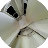
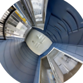
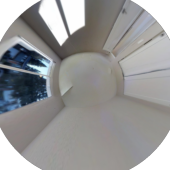
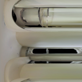
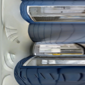
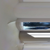
Figure 2: Example images collected via Habitat-Sim [habitat19iccv]. Top row: original images; Bottom row: images after linear-polar warping. From left to right: Delton, Montreal0, Pasatiempo0