The Hi-GAL compact source catalogue - II. The 360^∘ catalogue of clump physical properties

Abstract

We present the $360^{\circ}$ catalogue of physical properties of Hi-GAL compact sources, detected between 70 and 500 $\mu$m. This release not only completes the analogous catalogue previously produced by the Hi-GAL collaboration for $-71^{\circ}\lesssim\ell\lesssim 67^{\circ}$, but also meaningfully improves it thanks to a new set of heliocentric distances, 120808 in total. About a third of the 150223 entries are located in the newly added portion of the Galactic plane. A first classification based on detection at 70 $\mu$m as a signature of ongoing star-forming activity distinguishes between protostellar sources (23 per cent of the total) and starless sources, with the latter further classified as gravitationally bound (pre-stellar) or unbound. The integral of the spectral energy distribution, including ancillary photometry from $\lambda=21$ to 1100 $\mu$m, gives the source luminosity and other bolometric quantities, while a modified black body fitted to data for $\lambda\geq 160~{}\mu$m yields mass and temperature. All tabulated clump properties are then derived using photometry and heliocentric distance, where possible. Statistics of these quantities are discussed with respect to both source Galactic location and evolutionary stage. No strong differences in the distributions of evolutionary indicators are found between the inner and outer Galaxy. However, masses and densities in the inner Galaxy are on average significantly larger, resulting in a higher number of clumps that are candidates to host massive star formation. Median behaviour of distance-independent parameters tracing source evolutionary status is examined as a function of the Galactocentric radius, showing no clear evidence of correlation with spiral arm positions.

1 Introduction

The observational study of star formation makes use of both analysis of single objects and small regions and analysis of large surveys. These two approaches are complementary, because surveys provide observers with numerous targets to be inspected in more detail, e.g., by means of interferometric techniques. At the same time, large surveys produce a Galactic-scale view of star formation, which in turn represents a fundamental bridge between our knowledge of this phenomenon in the Milky Way and in external galaxies. Moreover, almost every recent article presenting studies of early phases of star formation based on infrared/sub-mm surveys begins with highlighting the importance of a statistical approach to address the formation of massive stars, which is still quite elusive because of intrinsically low incidence and relatively fast time scales. Notwithstanding, massive stars have significant feedback on the surrounding environment and hence the great interest. Among these surveys, Hi-GAL (Herschel InfraRed Galactic Plane Survey, Molinari et al., 2010) has a unique combination of characteristics favourable for systematically observing the early stages of star formation throughout the Milky Way. Hi-GAL was an Open Time Key Project that was granted about 1000 hours of observing time with the Herschel Space Observatory (Pilbratt et al., 2010), drawn from all three Herschel Announcements of Opportunity (KPAO, AO1, AO2) supplemented by Director’s Discretionary Time (DDT). Hi-GAL data were taken in parallel mode, using the two cameras on board Herschel: PACS (70 and 160 $\mu$m bands, Poglitsch et al., 2010) and SPIRE (250, 350 and 500 $\mu$m bands, Griffin et al., 2010). The uniqueness of Hi-GAL with respect to other Galaxy plane surveys in the continuum is threefold: ($i$) the wavelength range covered was crucial for studying the spectral energy distribution (SED) of cold dust, whose peak is expected to fall at $\lambda>100~{}\mu$m; ($ii$) the unprecedented sensitivity and dynamical range of the satellite-borne Herschel observations enabled the detection of both diffuse emission and faint compact sources; and ($iii$) the unbiased observation of the entire Galactic plane probed a statistically significant variety of environmental conditions across the Milky Way.

The first Hi-GAL instalment of observing time (AO) spanned the Galactic coordinate range $-71.0^{\circ}\lesssim\ell\lesssim 67.0^{\circ}$, $|b|<1.0^{\circ}$. For this area towards the inner Galaxy (somewhat inappropriately dubbed “inner Galaxy”, see Section 2.2), single-band photometric catalogues of compact sources (namely objects unresolved or poorly resolved in the maps) were delivered by Molinari et al. (2016a). Using this photometry, Elia et al. (2017, hereafter Paper I) compiled a catalogue of physical properties of sources with a reliable spectral energy distribution (SED).

In the present context of completion of the $360^{\circ}$ coverage of Hi-GAL, the work of Molinari et al. (in preparation) will represent the completion of the photometric catalogues of Molinari et al. (2016a), while this paper represents the completion of the physical source catalogue of Paper I, giving a global view of early phases of star formation across the whole Milky Way. Quantitatively, with this work we extend the longitude coverage of Paper I by a factor $\sim 2.6$ and increase the number of catalogued reliable compact sources from 100922 to 150223.

The main improvements and advances are as follows:

• For longitudes outside the range already published in Paper I, we present for the first time the catalogue of compact source physical properties and discuss their statistics, similarly to Paper I.

• For the longitude range already published in Paper I, we use a new set of source kinematic distances delivered by Mège et al. (2021), accordingly rescaling all of the distance-dependent parameters (such as sizes, masses, luminosities).

• It is now possible to discuss the distribution of such physical properties as a function of position in the Galaxy. In particular, we focus on comparison of overall statistics for the inner Galaxy and outer Galaxy, defined here by the radial zones in the latitude range covered that are inside and outside the Solar circle, respectively.

In Section 2 the procedures followed to build the catalogue are described briefly, referring the reader to Paper I for further details. Sections 3 and 4 focus on the statistics of distance-dependent and distance-independent parameters, respectively. In Section 5, global trends for such quantities as a function of the Galactocentric distance are discussed. Section 6 summarises our conclusions. Finally, Appendix A gives a detailed description of each catalogue column and Appendix  B contains a brief analysis of flux distributions for mid-infrared (MIR) counterparts of our Hi-GAL sources.

2 Building the catalogue

2.1 SED selection, classification, and fitting

The Hi-GAL SEDs were assembled, starting from the single-band photometry lists of Molinari et al. (in preparation) and adopting the same procedure used for Paper I. Here we briefly summarise the main steps and subsequent filtering, referring the reader to Paper I for further details.

• Only sources detected in the common area surveyed by both PACS and SPIRE cameras are considered for subsequent steps. For the observations already considered in Paper I, the boundaries of this area have been refined, being slightly but systematically enlarged. At the end of the selection process described below, this results in the inclusion of more than 1000 new sources at longitudes already covered in Paper I. This, and especially the adoption of a new set of heliocentric distances, lead us to discuss a new the statistics of source properties in this longitude range, an important part of the full catalogue.

• Sources detected at different Herschel bands are associated as counterparts of the same object simply based on position matching (see also Elia et al., 2013). Possible cases of multiplicity are resolved simply by keeping the closest counterpart. Only for the 70 $\mu$m and MIR ancillary bands (see below) is the total flux of all possible counterparts also computed, for use in calculating bolometric parameters.

• To filter SEDs as being suitable for fitting with a modified black body (hereafter MBB), SEDs are accepted as reliable by having at least three adjacent fluxes in the spectral range $160~{}\mu\mathrm{m}\leq\lambda\leq 500~{}\mu\mathrm{m}$, a concave-down shape, and $F_{350}-F_{500}>0$. This selects SEDs of 150223 sources.

  

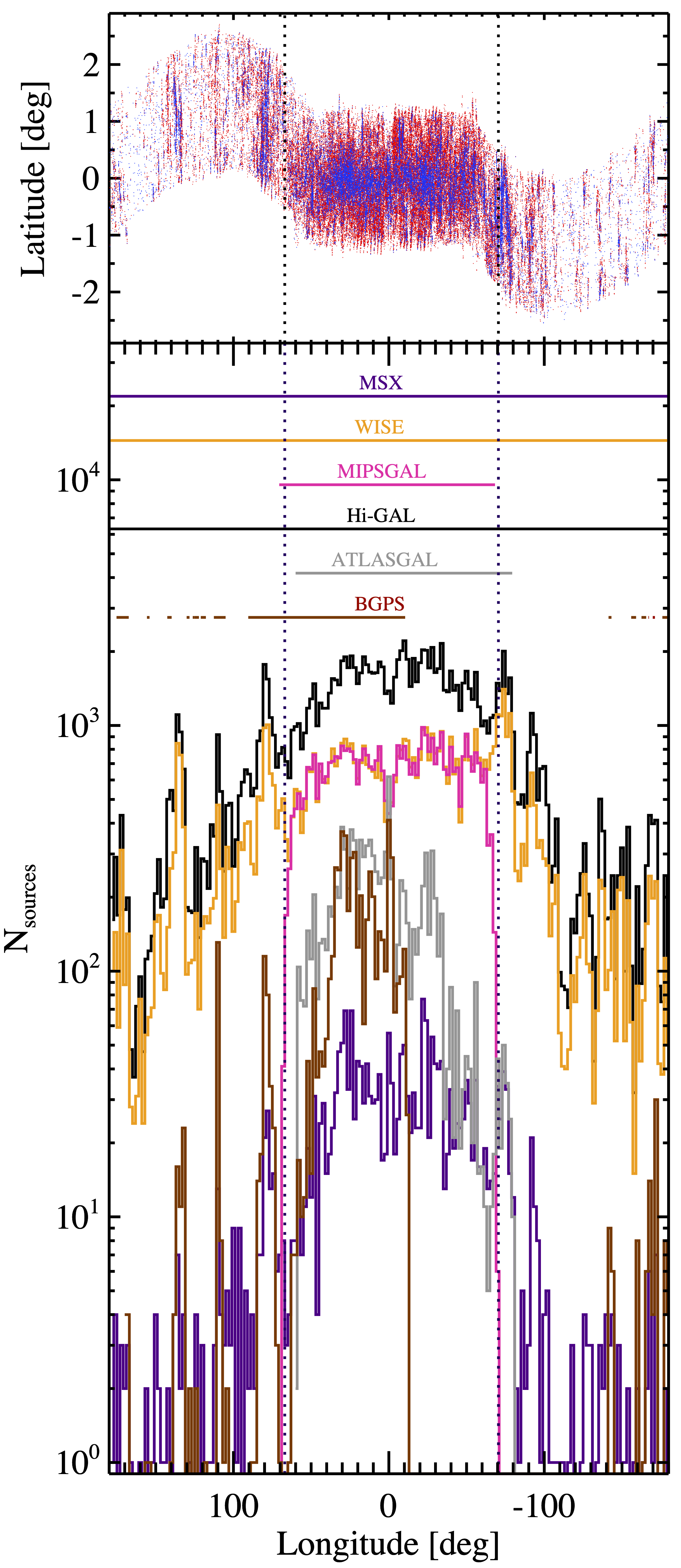
  Figure 1: Top panel: Positions ($\ell,b$) of Hi-GAL sources. To reduce crowding in the plot, only protostellar (blue) and pre-stellar (red) sources in the “high-reliability” catalogue are displayed. Bottom panel: histogram of Hi-GAL sources (black) in $2^{\circ}$-bins of Galactic longitude, together with histograms of counterparts found in the MSX (purple), WISE (orange), MIPSGAL (magenta), ATLASGAL (grey), and BGPS (brown) surveys, respectively. Local peaks (in logarithmic scale) in the outer Galaxy at about $-168^{\circ}$, $-154^{\circ}$, $-136^{\circ}$, $-92^{\circ}$, $-74^{\circ}$, $+80^{\circ}$, and $+136^{\circ}$, can be attributed to Gem OB1, Rosette, CMA OB1, Vela C, Cygnus-X, and W3/W4/W5 regions, respectively. In the upper part of the panel, the longitude coverage for each survey is also shown. Dotted vertical lines crossing both panels delimit the longitude range already presented in Paper I.

• With the same procedure used in Paper I, counterparts to the Hi-GAL sources at 21, 22, 24, 870 and 1100 $\mu$m have been found in the MSX (Egan et al., 2003), WISE (Wright et al., 2010), MIPSGAL (Gutermuth & Heyer, 2015), ATLASGAL (Schuller et al., 2009; Csengeri et al., 2014), and BGPS (Rosolowsky et al., 2010; Ginsburg et al., 2013) catalogues, respectively. The coverage of the outer Galaxy is full for MSX and WISE, and poor or even missing for the other surveys (Fig. 1). While we used photometry from sub-millimetre surveys to better constrain the MBB fit (see below), MIR fluxes, where available, were used instead to quantify the excess of emission with respect to such a fit, which can significantly increase the estimates of bolometric quantities (see below). In this respect, MSX and WISE compensate for the unavailability of MIPSGAL in the outer Galaxy, ensuring a uniformity between the inner and outer Galaxy, at least for sources brighter than 0.1 Jy (see Appendix B, Fig. 29). The same applies for areas severely saturated in MIPSGAL (see, e.g., the dip around $\ell=0^{\circ}$ in the distribution of MIPSGAL sources in Fig. 1, bottom).

  

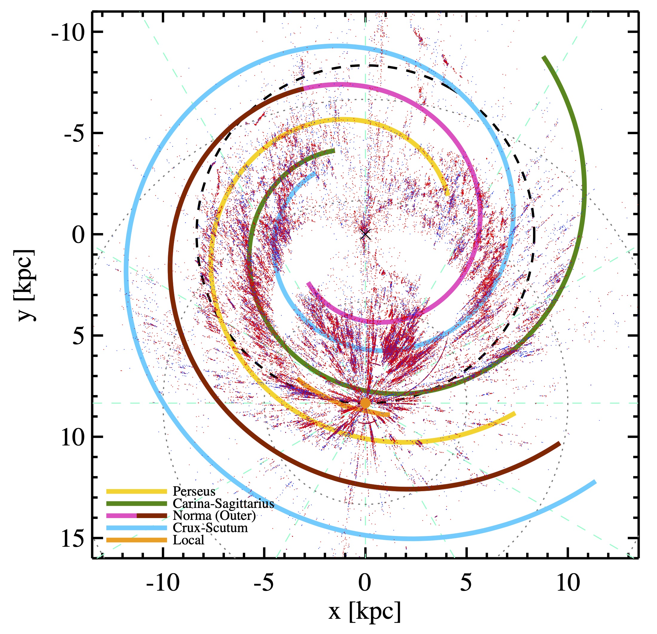
  Figure 2: Positions projected in the Galactic plane for the pre-stellar (red dots) and protostellar (blue dots) Hi-GAL objects with a known distance (unbound objects not shown to reduce crowding). The Galactic centre at coordinates $[x,y]=[0,0]$ is indicated with a $\times$, and the Sun at [0,8.34] kpc with an orange dot. Some unnatural delineation of an imaginary circle passing through the Sun and Galactic centre arises from sources placed arbitrarily at the tangent point in the heliocentric distance estimates by Mège et al. (2021), see the text. Cyan dashed lines indicate Galactic longitude in steps of $30^{\circ}$. The Solar circle, separating the “inner” from “outer” Galaxy, is represented with a black dashed circle. Grey dotted circles represent heliocentric distances of 5, 10, and 15 kpc. Spiral arms from the four-arm Milky Way prescription of Hou et al. (2009) are plotted, except for the Local arm taken from Xu et al. (2016), with the arm-colour correspondence at the bottom left.The Norma arm is represented using two colours: magenta for the inner part; and brown for the outer part, which is generally designated as the Outer arm, whose starting point is established in agreement with Momany et al. (2006). The uniform line thickness is not representative of the actual arm widths.

• Source heliocentric distances were determined by Mège et al. (2021), who developed a new code for assigning a $V_{\mathrm{LSR}}$ to each Hi-GAL source, using all the available spectroscopic data complemented by a morphological analysis to choose the best velocity in presence of multiple spectral components along the line of sight. This analysis is based on considerations on the spatial distribution of molecular emission, rather than simply on its brightness. Once the velocity is determined, if no stellar or maser parallax distance is known, the kinematic distance is calculated and the near/far distance ambiguity inside the Solar circle is solved with the H i self-absorption method or from distance–extinction data. This procedure is similar to that of Russeil et al. (2011) which provided us with distances for Paper I, but with substantial improvements in the $V_{\mathrm{LSR}}$ assignment criteria. Furthermore, the spectroscopic data base was considerably updated, and a new rotation curve adopted (Russeil et al., 2017). In particular, we adopted their distance list based on line detection in molecular spectra at a $3-\sigma$ level (where $\sigma$ represents the noise level of each spectrum). From this set of distances, we rejected ($i$) those corresponding to a Galactocentric distance $R_{\mathrm{GC}}>20$ kpc, and ($ii$) those placed at the distance of the tangent point because of a kinematically forbidden $V_{\mathrm{LSR}}$, but having a velocity differing by more than 10 km s^-1 from that of the tangent point. After this selection, valid distances were assigned to 120808 sources, whose positions are shown in Fig. 2. Statistics are reported in Tables 1 and 2. A more detailed discussion about distances is postponed to Section 3.1.

• A MBB with constant emissivity index $\beta=2$ was fitted to SED data at $\lambda\geq 160~{}\mu$m to estimate the total mass and average temperature of the clump. Two different expressions for the MBB were used: one explicitly containing the optical depth $\tau_{\lambda}$ (e.g., Elia & Pezzuto, 2016, their Equation 3) and one assuming optically thin emission at all wavelengths (their Equation 8). The former is preferred if the free parameter, wavelength $\lambda_{0}$ for which $\tau_{\lambda_{0}}=1$ is less than than 50.6 $\mu$m, based on considerations described in Paper I. Otherwise, the physical parameters are derived with the latter. Subsequently, for calculating bolometric temperature and luminosity, integrals based on the analytical best-fitting MBB are considered for pre-stellar sources. However, for a protostellar source the integral of the MBB for only $\lambda\geq 160~{}\mu$m is combined with fluxes observed at shorter wavelengths (PACS at 70 $\mu$m and, if available, MSX, WISE, and MIPSGAL). For sources without a distance estimate, the fit was still performed in order to compute the distance-independent parameters. Distance-dependent parameters were calculated for a hypothetical distance of 1 kpc and appropriately flagged in the catalogue (see Appendix A).

• The properties calculated through the fit of SEDs with fluxes in at least four Herschel bands are generally considered “highly reliable”. The corresponding sources are included in the main catalogue, with the exception of cases in which the results of the best-$\chi^{2}$ fit corresponded to the extreme values explored for the temperature, namely 5 and 40 K, which might be the result of a failed fit. These exceptions are relegated to the “low-reliability” source catalogue. Sources with only three fluxes (which are necessarily starless, by construction) have properties derived from a poorly constrained fit and are also reported in the “low-reliability” source catalogue. These catalogues contain 94604 and 55619 sources, respectively. Subsequent discussion in this paper is based entirely on the “high-reliability” catalogue, except in cases where it is stated explicitly that both catalogues are used.

• An overall classification distinguishing clumps containing star formation activity (protostellar) versus quiescent clumps (starless) is based on the presence or not, respectively, of a detection at $70~{}\mu$m. This classification makes use of only Herschel photometry and, as widely discussed in Paper I and Baldeschi et al. (2017a), can be affected by confusion and/or lack of sensitivity at $70~{}\mu$m (for $F_{70}\lesssim 0.2$ Jy). The first effect is due to lack of spatial resolution at increasing distance, so that the $70~{}\mu$m-emission produced by a limited fraction within a given clump is assigned to the entire object, to which a protostellar classification is then given. The second effect goes opposite to the previous one, because it leads to misclassify sources with a true star formation content as starless. In particular, low-mass Class 0 objects are known to have low luminosities (Dunham et al., 2013), so their possible contribution to the clump emission at 70 $\mu$m may remain undetected. In fact, spectroscopic signatures of ongoing star formation have been found in small samples of $70~{}\mu$m-quiet Herschel clumps, both infall (e.g., Traficante et al., 2017) and outflow (e.g., Duarte-Cabral et al., 2013). In this respect, starless sources should be more rigorously named candidate starless clumps. We refer the reader to Appendix C of Paper I and to Section 3.1 of this paper for a further discussion of the combined effect of these two biases.

• Finally, starless clumps are further classified as gravitationally bound (hereafter pre-stellar) or unbound, using the so-called “Larson’s third law”, $M(r)=460~{}M_{\odot}~{}(r/\mathrm{pc})^{1.9}$ (Larson, 1981), as a threshold to divide the $M$-$r$ plane, where $M$ and $r$ are the source mass and physical radius, respectively. It is necessary to point out that this classification is based only on considerations about gravitational stability. However, gravitationally unbound sources can be confined by external pressure (e.g., Kainulainen et al., 2011). A complete virial analysis for clumps (see, e.g., Pattle, 2016) would require information about external pressure, together with magnetic field and total internal kinetic energy (including turbulence), and is beyond the scope of this paper, which is essentially based on photometric observations only.

The coordinates of protostellar and pre-stellar clumps contained in the “high-reliability catalogue” are shown in the top panel of Fig. 1, from which it is evident how the Hi-GAL coverage followed the Galactic warp in the outer Galaxy. Furthermore, in Fig. 3 the distribution of the Hi-GAL sources in the Galactic plane (already shown in Fig. 2) is rendered through source density contours for the different classes. No particular behaviour is seen for different source populations with respect to spiral arm locations.

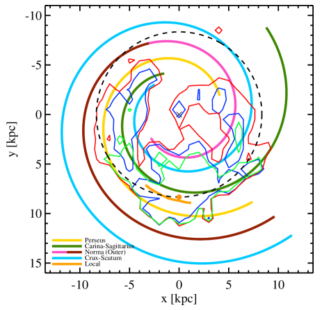
Figure 3: The same as Figure 2, but with source density contours displayed instead of source positions. Sources are counted in boxes of 1 kpc². To avoid figure crowding, only one contour, corresponding to a level of 100 sources kpc^-2 is plotted for each source class: green for starless unbound sources (not shown in Figure 2), red for pre-stellar, and blue for protostellar, respectively.

2.2 “Inner” vs “outer” Galaxy

In this paper, a systematic comparison between properties of Hi-GAL sources in the “inner Galaxy” and “outer Galaxy” is carried out. In previous Hi-GAL literature “inner Galaxy” has generally been used to indicate the first tranche of the survey corresponding to the Herschel KPAO cycle, and published in Paper I. These observations, initially intended to span the $|\ell|<60^{\circ}$ longitude range, were actually extended to the $-71.0^{\circ}\lesssim\ell\lesssim 67.0^{\circ}$ range, corresponding to Hi-GAL tiles from $\ell$290 to $\ell$066 (according to the Hi-GAL nomenclature). Keeping this definition of “inner Galaxy” would allow a direct and easy comparison with Paper I.

However, this longitude range also contains sources located outside the Solar circle. Therefore, to avoid a quite arbitrary and counter-intuitive inner/outer division here we prefer to adopt a different more natural definition, “inner Galaxy” and “outer Galax” being the regions respectively inside or outside the Solar circle, 8.34 kpc as adopted by Mège et al. (2021). This definition, which applies to sources with a distance (and then Galactocentric radius) determination, gives 88131 and 32677 sources in the inner and in the outer Galaxy, respectively.

A classification for sources without a distance estimate can be attempted as follows. First, sources in the second and third Galactic quadrants are definitely located outside the Solar circle. However, sources in the first and fourth quadrants can belong to either the inner or outer Galaxy.

Histograms of the number of sources in $1^{\circ}$-bins of longitude (see Fig. 4, in which for the sake of clarity $2^{\circ}$-bins are shown), for sources with distances inside or outside the Solar circle, and for sources with no distance estimate, can be used to establish a rough criterion for assigning the latter sources in the first and fourth quadrants to either the inner or outer Galaxy for further analyses. In longitude bins in which the inner Galaxy sources outnumber the outer Galaxy sources “inner” is assigned, otherwise “outer” (which as might be expected occurs only near $\ell\pm 90^{\circ}$).

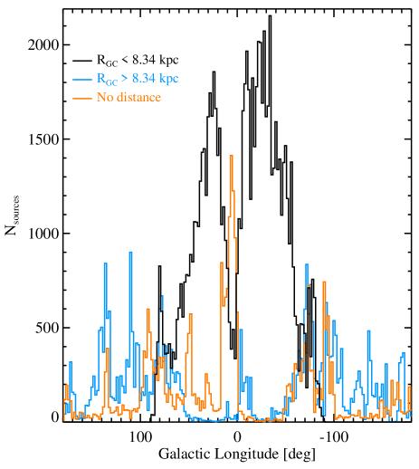
Figure 4: Histograms in $2^{\circ}$-bins of Galactic longitude of Hi-GAL sources located inside the Solar circle (black), outside (light blue), and lacking a distance/Galactocentric radius estimate (orange), respectively.

Table 1: Number of sources in the 360^∘ catalogue with high-reliability parameters, subdivided by evolutionary class and inner/outer Galaxy location.

	Inner Galaxy		Outer Galaxy		Total
	w/ distance	w/o distance	w/ distance	w/o distance
Protostellar	22132	5476	7572	6	35186
Pre-stellar	32013	8589	8683	4	49289
Unbound	3476	3033	3613	7	10129
Total	57621	17098	19868	17	94604

Table 2: Number of sources in the 360^∘ catalogue with low-reliability parameters, subdivided by evolutionary class and inner/outer Galaxy location.

	Inner Galaxy		Outer Galaxy		Total
	w/ distance	w/o distance	w/ distance	w/o distance
Protostellar	166	27	33	0	226
Pre-stellar	20705	5250	5308	2	31265
Unbound	9639	7007	7468	14	24128
Total	30510	12284	12809	16	55619

The total numbers of sources, separated by different evolutionary classes and by inner/outer Galaxy location, are reported in Table 1 for the “high-reliability” catalogue, and in Table 2 for the “low-reliability” catalogue, respectively.

3 Distance-dependent parameters

3.1 Heliocentric distance and Galactocentric radius

The heliocentric distance is a crucial parameter for characterizing the detected compact sources, not only to compute quantities depending directly on distance, such as physical size, mass and luminosity (see a dedicated discussion in Baldeschi et al., 2017a; Baldeschi et al., 2017b), but also to understand what meaning we can ascribe to other quantities that are formally distance-independent, especially when distant sources are actually the combination/blending of unresolved structures.

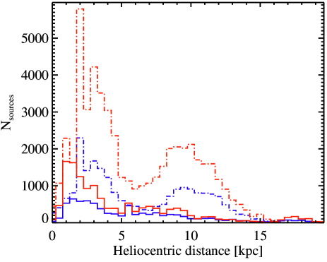
Figure 5: Top panel: number counts vs heliocentric distance for Hi-GAL pre-stellar (red) and protostellar (blue) clumps taken from both catalogues. Dot-dashed lines are used for distributions corresponding to the inner Galaxy, and solid lines for the outer one. Bottom panel: number ratio of pre-stellar to protostellar sources in the distance bins defined in the top panel, for the inner (dot-dashed) and the outer Galaxy (solid). To ensure statistical reliability, only bins in which both numerator and denominator are larger than 50 are reported, resulting in a foreshortened $x$-axis.

Adoption of the new distance set of Mège et al. (2021) significantly increases the number of catalogue sources with a known distance, in both absolute and relative terms: now 120808 out of 150223 (80 per cent) compared with Paper I, 57065 out of 100922 ($57$ per cent).

Figure 5, top, shows number counts vs heliocentric distance for our sample of objects (top panel), divided according to pre-stellar vs protostellar and inner vs outer Galaxy. Sources are included from both catalogues, i.e., regardless of the reliability of their SEDs, because distance determination is independent of the SED fit. The histograms for the inner Galaxy look bimodal (cf. Urquhart et al., 2013a), mostly due to near/far distance ambiguity present at those longitudes; this is not seen in the outer Galaxy, where most sources are found to be located within 10 kpc.

Figure 5, bottom, shows that pre-stellar sources are generally more abundant than protostellar sources at most distances in both the inner and outer Galaxy. However, the pre-stellar/protostellar number ratio seems to decrease at increasing distance, albeit with considerable scatter. Two competing effects can affect this ratio at large distances: on the one hand, insufficient PACS sensitivity at 70 $\mu$m may lead to misclassifying protostellar sources as pre-stellar; on the other hand, source confusion with possible blending of pre-stellar and protostellar sources may result in a single object classified as protostellar (see Paper I, Appendix C1). The trend seen is consistent with the latter effect being predominant. Considering all sources in the outer Galaxy, the percentage classified as protostellar is 47 per cent; this is slightly higher than the corresponding number in the inner Galaxy, 40 per cent.

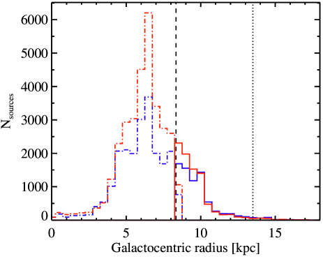
Figure 6: Same as Fig. 5, top panel, but for Galactocentric radius. The vertical dashed and dotted lines delimit the outer Galaxy and the so-called far outer Galaxy ($R_{\mathrm{GC}}>13.5$ kpc), respectively.

Figure 6 presents number counts vs Galactocentric radius $R_{\mathrm{GC}}$, which is not affected by the near/far distance ambiguity. The peak at about 6 kpc in the inner Galaxy, seen also by Ragan et al. (2016) based on the previous set of Hi-GAL distances and by Wienen et al. (2015) for ATLASGAL sources, is compatible with the position of the so-called “molecular ring” (e.g., Dobbs & Burkert, 2012; Miville-Deschênes et al., 2017). Other local peaks are present at about 8.5 kpc and 10-11 kpc in the outer Galaxy. In Schlingman et al. (2011) these three features, observed over a sample of a few hundred BGPS sources, are associated with the Sagittarius, Local, and Perseus arms, respectively. However, a feature around 4.5 kpc attributed by Schlingman et al. (2011) and Wienen et al. (2015) to the closer tip of the Galactic bar is not prominent in our data, which in general appears smoother due to the large number of inter-arm sources in our catalogue (Fig. 2).

Figure 7: Number counts in $2^{\circ}$-bins of Galactic longitude of Hi-GAL sources located in the FOG ($R_{\mathrm{GC}}>13.5$ kpc). Both pre-stellar and protostellar sources are counted, from both catalogues. The $x$-axis range is set from $-90^{\circ}$ to $270^{\circ}$ in order to place the local peaks around $0^{\circ}$ and $180^{\circ}$ well inside the plot area.

Finally, we discuss the ability of the PACS and SPIRE cameras (but also of line surveys used to determine distances) to detect sources in the far outer Galaxy (hereafter FOG). Various boundaries for the FOG, in terms on $R_{\textrm{GC}}$, are found in the literature, such as 13.5 (Heyer et al., 1998), 15 (Honma et al., 2011), and 16 kpc (Urquhart et al., 2013a), all of which are well outside the ranges of $R_{\textrm{GC}}$ probed by the aforementioned ATLASGAL and BGPS surveys. But for Hi-GAL, Fig. 6 suggests that a small but meaningful number of clumps, essentially contained in the range 13.5 kpc $<R_{\textrm{GC}}<$ 15 kpc, deserves attention. Considering sources at $R_{\textrm{GC}}\geq 13.5$ kpc, and including both catalogues, we find that 967 sources lie in the FOG. However, it is evident from Fig. 7 that many of these large $R_{\textrm{GC}}$ values come from lines of sight close to the Galactic centre and anti-centre, areas suffering from large uncertainties in kinematic distances. Neglecting sources with $|\ell|<10^{\circ}$ or $|\ell-180^{\circ}|<10^{\circ}$, 677 sources remain. The prominent peak around $\ell\sim 212^{\circ}$ is from sources found by Mège et al. (2021) to be associated with the Sh2-284 H ii region; the adopted heliocentric distance 6.6 kpc yields $R_{\textrm{GC}}=14.4$ kpc. Most of the remaining sources are concentrated in the second quadrant. A brief analysis of the physical properties for sources in the FOG is given in Section 5.

3.2 Physical size

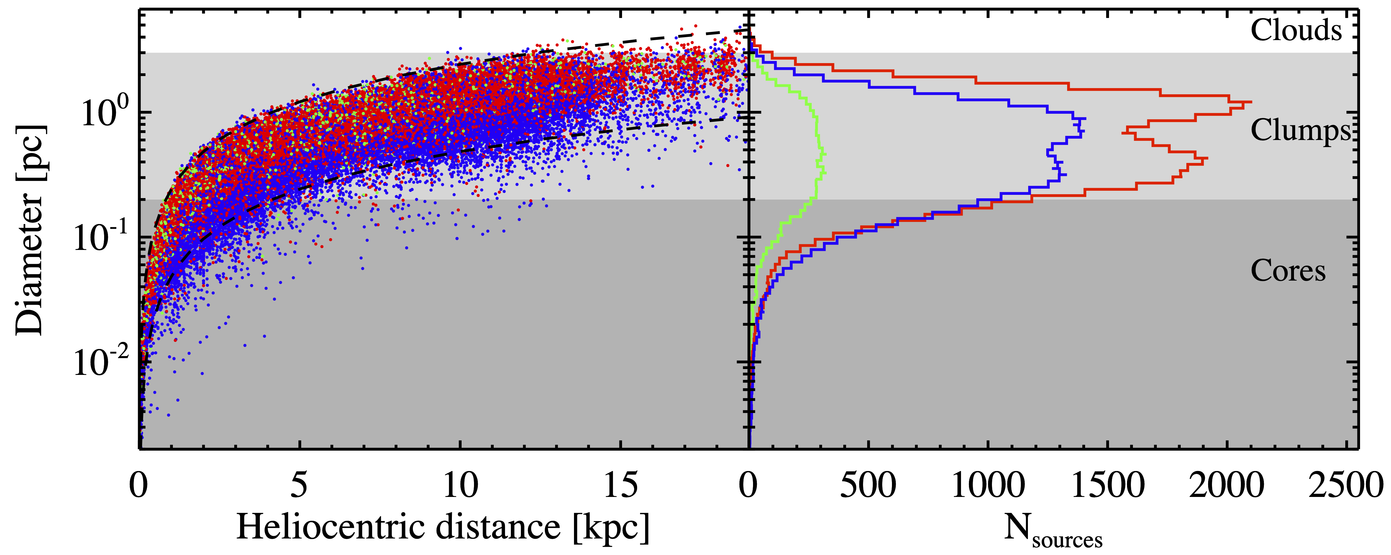
Figure 8: Left-hand panel: Hi-GAL clump linear diameters, obtained by combining distance and angular size estimated at 250 $\mu$m as explained in Appendix A, versus distances (blue: protostellar; red: pre-stellar; green: starless unbound). Different background tones of grey indicate ranges of diameter corresponding to different object classifications labelled at the right (see Section 3.2). Upper and lower dashed lines correspond to an angular size of 50 and 10 arcsec, respectively. Right-hand panel: distribution of source diameters for protostellar, pre-stellar, and starless unbound sources, rotated to share the $y$-axis and background colours with the left-hand panel. Line colours also the same encoding of source classification.

Estimating the physical size of compact sources is of great importance to understanding the nature of objects investigated. Paper I showed that most Hi-GAL sources fulfil the definition of clumps ($0.2~{}\mathrm{pc}<D<3~{}\mathrm{pc}$, based on Bergin & Tafalla, 2007, where $D$ is the diameter of the structure), while a smaller fraction of nearby sources can be classified as cores, i.e., condensations supposed to host (or be progenitors of) formation of a single star or small stellar system.

Figure 8 reports the same information as in Paper I, updated with new distances and extended to the entire $360^{\circ}$ survey coverage. Trends seen in Paper I are basically confirmed. On average, protostellar sources are more compact than pre-stellar sources (left-hand panel). Most sources (80.1 per cent) can be classified as clumps, so that hereafter we often refer to all sources as “clumps”. Only 19.7 per cent and 0.3 per cent of sources fulfill the Bergin & Tafalla (2007) definition of cores and clouds, respectively (right-hand panel). The bi-modality that appears in the distributions of both pre-stellar and protostellar sources is a direct consequence of the bi-modality in distances seen in the upper panel of Fig. 5.

3.3 Mass vs radius

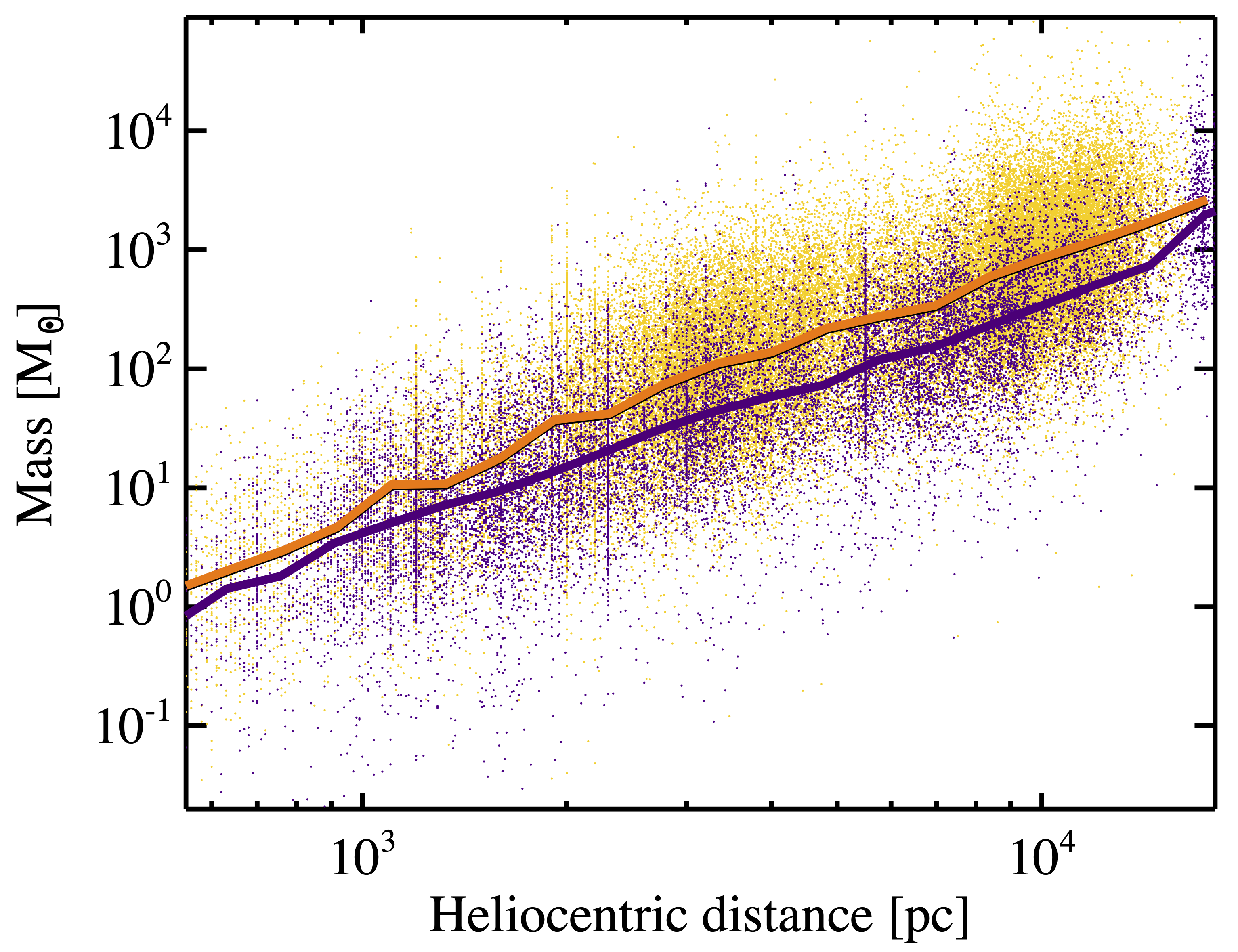
Figure 9: Clump mass vs heliocentric distance for sources in the inner (orange dots) and in the outer Galaxy (purple dots). Orange and purple thick lines represent the median mass in logarithmic bins of distance for these two populations, respectively.

The clump mass depends on the square of the estimated heliocentric distance. Moreover, the selection effect, known as Malmquist bias (see, e.g., Zetterlund et al., 2018), favours detection of larger and larger masses and luminosities at increasing distance. Such bias affects not only the completeness of the observed sample, but also the nature of the objects included: for a very distant source whose internal structure cannot be resolved with Herschel, the total derived mass (even $M>10^{5}M_{\odot}$) does not describe an entity forming a single star, but rather a large and complex structure hosting several compact sources (see, e.g., Baldeschi et al., 2017a). For this reason, here we avoid considering an overall mass function for Galactic clumps regardless to their distance (it is more reasonable to consider it within bins of distance as in Paper I, ) or drawing up any ranking of the most massive clumps in the Galaxy.

Distance bias has to be taken into account in a global comparison of the masses encountered in the inner and outer Galaxy, given the different ranges of distances found in Section 3.1 for inner versus outer. However, the deficiency of large masses in the outer Galaxy compared to the inner Galaxy appears to be intrinsic: considering common bins of heliocentric distance, Fig. 9 shows that the median mass of sources in the outer Galaxy is always smaller (by a factor ranging from 1.1 to 4.3) than the corresponding median for the inner Galaxy. The largest distance bin, $d\gtrsim 16$ kpc, could be misleading: sources far behind the Galactic centre, thus entirely in the outer Galaxy, also have high mass estimates due to their relatively large distances, and so any highly uncertain distance assignments could lead to the upturn in the purple curve.

This general trend of larger clump masses in the inner Galaxy compared with the outer Galaxy was already suggested by Zahorecz et al. (2016) (but based on a much smaller statistical sample), and can be understood as being the result of the essentially different regime of surface density found in Section 4.5. This point will be addressed in Section 5.

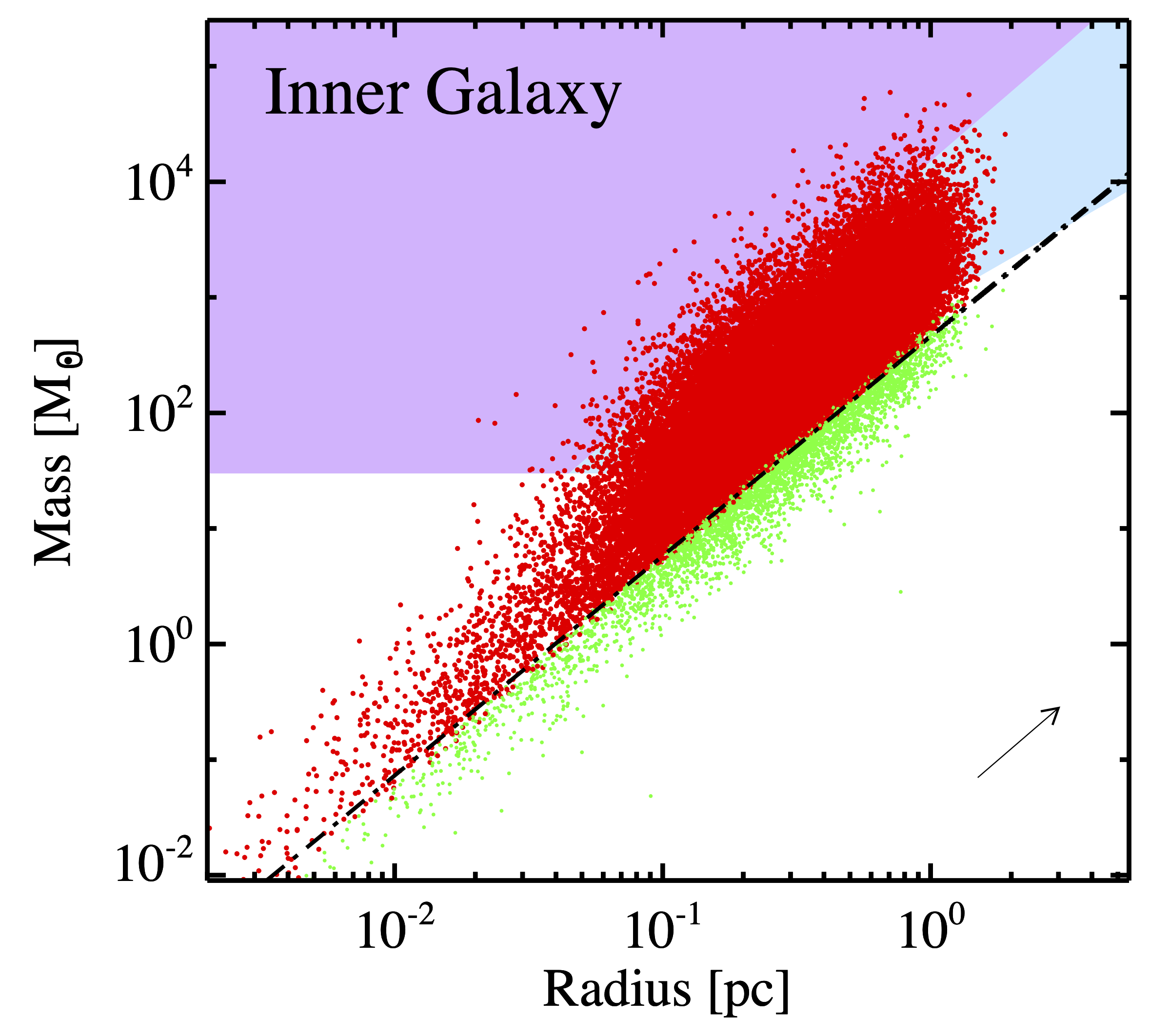
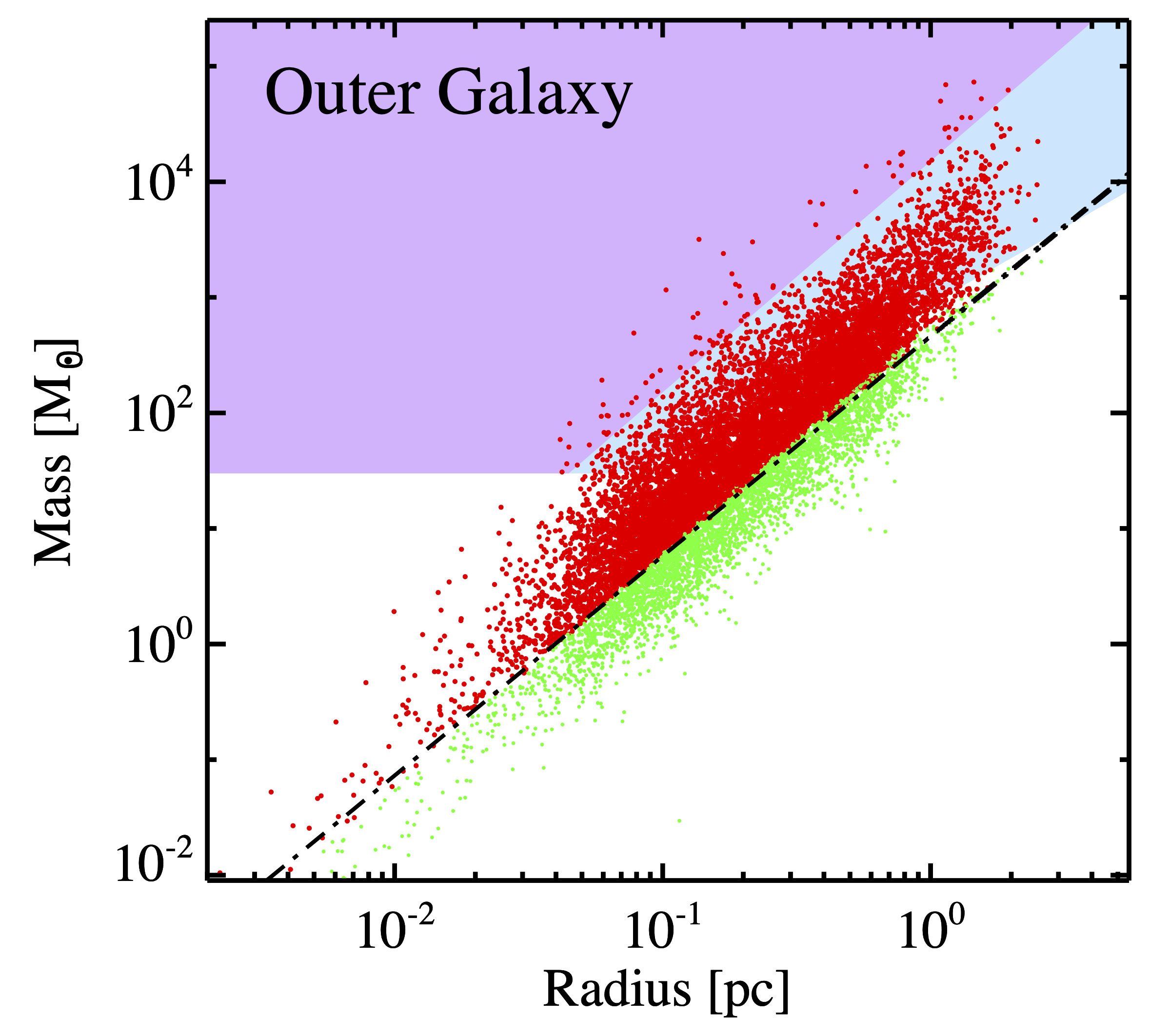
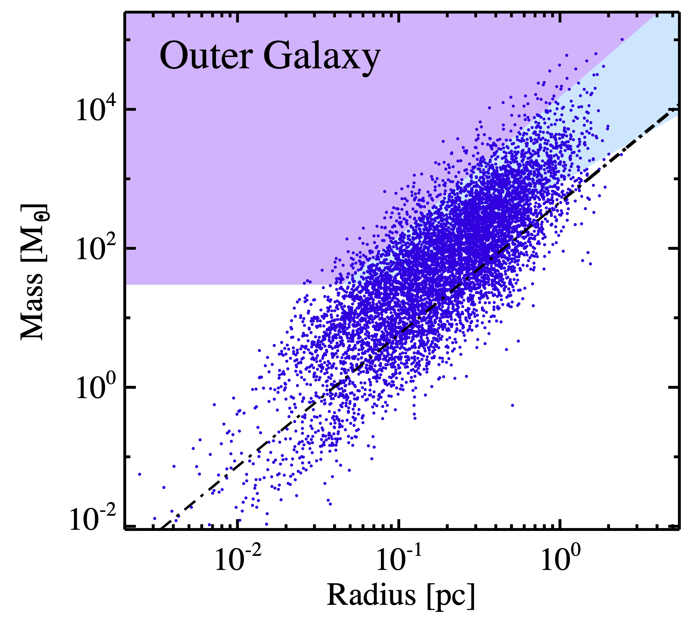
Figure 10: Mass vs radius plot for starless sources in the inner (top left-hand panel) and outer Galaxy (bottom left), and for protostellar sources in the inner (top right) and outer Galaxy (bottom right). Uncertainty in distance is the main source of error on both displayed quantities and the shift corresponding to a hypothetical distance increase of a factor 2 is shown as an arrow at the bottom right corner of the top left panel. In the left two panels containing starless sources, the dot-dashed black line $M(r)=460~{}M_{\odot}~{}(r/\mathrm{pc})^{1.9}$ (Larson, 1981, see Section 2.1) separates pre-stellar (red) and unbound (green) sources. The area in each diagram fulfilling the Krumholz & McKee (2008) threshold for compatibility with high-mass star formation is shaded purple, and the less demanding Kauffmann & Pillai (2010) threshold contains this and extends it as indicated in light blue. Adopting $10~{}M_{\odot}$ as a lower limit for a massive star, and a star formation efficiency factor of $1/3$ for the core-to-star mass transfer as in Elia et al. (2013), these shaded areas cannot extend below $30~{}M_{\odot}$.

Studying the gravitational stability of sources or their ability to form high-mass stars requires a combination of information about mass and size, as we will discuss with Fig. 10. Note that the relation between these two estimated quantities is still distance-dependent, because they scale with distance quadratically and linearly, respectively. Moreover, in most cases the catalogued radius and mass represent overall summary observables for clumps hosting an unresolved complex morphology, so that any inference about gravitational stability should be taken as a large-scale description of a clump, while also keeping in mind that large fluctuations in density are possible inside the object.

By plotting mass versus radius in Fig. 10 separately for inner and outer Galaxy sources we can appreciate that larger values of mass are achieved in the inner Galaxy, as already seen in Fig. 9. In the two panels on the left for starless sources it is possible to visualise how the “Larson’s third law” is used to separate gravitationally bound (pre-stellar) from unbound sources (see Section 2.1), determining the statistics reported in Tables 1 and 2. We point out that, strictly speaking, this kind of analysis should apply only to the pre-stellar sources, whose properties correspond to conditions prior to the onset of star formation. Protostellar sources, on the other hand, have already experienced a mass transfer on to the forming star(s) and partial envelope dissipation, whose extent depends in principle on their individual evolutionary stage. Their masses therefore represent lower limits for the original ones.

Table 3: Number of Hi-GAL sources in the inner or outer Galaxy having a mass-radius combination that is compatible with massive star formation according to five different increasingly-demanding thresholds (see the text).

	Ur14		KP10		Ba17		KM08		Br12
	inner	outer	inner	outer	inner	outer	inner	outer	inner	outer
Protostellar	16596	4013	13728	2827	12369	2330	3027	298	27	9
Pre-stellar	25503	5101	18207	2756	14758	1974	1156	88	12	9
Total	42099	9114	31935	5583	27127	4304	4183	386	39	18

As in Paper I, we discuss the regions of the mass versus radius plot corresponding to conditions that from time to time have been considered necessary but not sufficient to have high-mass star formation inside the clumps. In particular, in Fig. 10 we show the area defined by the theoretical threshold of Krumholz & McKee (2008), corresponding to a clump surface density $\Sigma=1$ g cm^-2, and how this area is extended using the empirical and less demanding threshold by Kauffmann & Pillai (2010). In Table 3, we report statistics of pre-stellar and protostellar sources, in the inner and in the outer Galaxy, fulfilling these two thresholds (indicated with “KM08” and “KP10”, respectively). Notice that the total number of sources above the KM08 threshold represents the 4 per cent of the entire catalogue, which is comparable with the 6 per cent level found by Merello et al. (2015) on a sample of 286 sources observed with SHARC-II (Dowell et al., 2003).

Subsequently, KM08 has been demonstrated to be too conservative when compared with observations: López-Sepulcre et al. (2010), Butler & Tan (2012), Peretto et al. (2013), Tan et al. (2013), Urquhart et al. (2014), and Traficante et al. (2018) report high-mass star formation even for surface densities in the range $0.05\leq\Sigma\leq 0.5$ g cm^-2. In particular, the numbers of sources fulfilling the less demanding value, 0.05 g cm^-2 by Urquhart et al. (2014) are reported in Table 3, column “Ur14”.

It is to notice that this proliferation of thresholds reflects a variety of observational conditions, and of adopted criteria. Instead of making a comparison with them, it may be possible, in turn, to extrapolate a threshold directly from our data, by comparison with a sample of well-known high-mass star forming objects. However, this is beyond the scope of this paper. Anyway, a specific analysis for the case of Hi-GAL observations was carried out by Baldeschi et al. (2017a), who evaluated the bias introduced by distance in classifying Herschel sources as potentially able to form high-mass stars. They suggested another power-law threshold with slope 1.42, i.e., between 2 (KM08) and 1.33 (KP10) but much closer to the latter. Source numbers corresponding to this threshold are also reported in Table 3, column “Ba17”.

For all four thresholds there are impressively high numbers of sources, both pre-stellar and protostellar, that can be considered as candidates for high-mass star formation. In the inner Galaxy the numbers of candidates for the KP10, Ba17, and KM08 thresholds have all increased systematically compared with Paper I, despite a slightly smaller total number of sources because of the different definition of inner Galaxy adopted in this paper (Section 2.2). These increased numbers are due mostly to the increase of the number of sources having a distance estimate in this work, rather than an increasing fraction of sources being candidates. For example, for sources having a distance estimate in Paper I the fraction of sources fulfilling the KP10 threshold was 71 per cent and 65 per cent of the total protostellar and pre-stellar sources, respectively. The new numbers reported in Table 3 correspond to 62 per cent and 56 per cent, respectively, of the larger totals having distances, i.e., lower percentages than in Paper I.

While this direct comparison with Paper I is perfectly feasible and consistent since the same dust opacity has been used, further comparisons with similar mass-radius plots (e.g., that of Svoboda et al., 2016) are more complicated because they would imply to re-scale our masses taking into account different opacities adopted. Svoboda et al. (2016) clearly showed that numbers of sources compatible with massive star formation according to a given threshold should be computed as a function of the adopted opacity. Furthermore, Paper I highlighted that the range of typically used reference opacities would correspond to a scaling factor from 0.6 to 6 for masses. Therefore if, for example, we simply change the value of the reference opacity (which is 0.1 cm² g^-1 at 300 $\mu$m, see Paper I, ) to that predicted at the same wavelength by the OH5 model of Ossenkopf & Henning (1994) adopted by Svoboda et al. (2016), a factor 0.77 should be applied to our masses. The consequent fraction of sources fulfilling the KP10 threshold would drop from 62 to 55 per cent for the protostellar class, and from 56 to 47 per cent for the pre-stellar class, respectively.

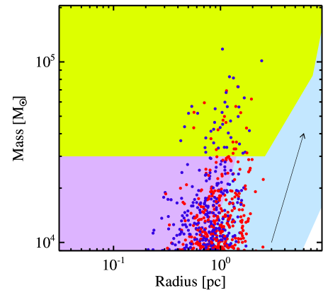
Figure 11: Mass vs radius for pre-stellar (red) and protostellar (blue) sources in the high-mass regime. As in Fig. 10, the shift corresponding to a hypothetical distance increase of a factor 2 is shown as an arrow. Purple and light blue areas are as introduced in Fig. 10. The overlying yellow sub-area towards high mass corresponds to the Bressert et al. (2012) threshold for identifying candidate massive proto-clusters.

Finally, we investigated the threshold proposed by Bressert et al. (2012) for identifying massive proto-cluster candidates, such that the content in stars would amount to $>10^{4}~{}M_{\odot}$ (Portegies Zwart et al., 2010). For $r<2.6$ pc, they establish a minimum mass of $3\times 10^{4}~{}M_{\odot}$ (corresponding to star formation efficiency 1/3), which is shown in Fig. 11. Clumps in our sample have $r<2.6$ pc, similar to the Galactic sources of Bressert et al. (2012), because surveys like Hi-GAL or ATLASGAL, resolve regions with a size of a several pc into smaller structures. As recorded in Table 3, last column “Br12”, we found 57 sources fulfilling this criterion, 18 of which are located in the outer Galaxy. Note that uncertainties in the source distances can have a strong influence on this classification. For example, in Fig. 11 a decrease of a factor 2 in the distances of all sources would empty the Bressert et al. (2012) area almost completely (see magnitude of arrow), while the opposite would populate it with hundreds more sources. A specific analysis of the 57 candidate proto-clusters is reserved for future work, being beyond the scope of this paper

3.4 Luminosity vs mass

In this section we expand on the discussion of the bolometric luminosity versus envelope mass ($L_{\mathrm{bol}}$ vs $M$) diagram given in Paper I, to which the reader is referred for further details and previous literature. This diagram is useful as an evolutionary diagnostic tool, when theoretical evolutionary tracks, taking into account an accretion phase and a clean-up phase (Molinari et al., 2008; Smith, 2014), are over-plotted for comparison to the data.

The $L_{\mathrm{bol}}$ vs $M$ plot for sources in the inner Galaxy is presented again here (Fig. 12, top), because of changes in distances and the different operational definition of inner Galaxy adopted here. Postponing quantitative considerations to Section 4.1, in which the ratio of $L_{\mathrm{bol}}$ to $M$ is used to summarise the relation between these two quantities for different populations, here we simply note that Fig. 12 is qualitatively very similar to the corresponding plot in Paper I. Again, a high degree of segregation is found between pre-stellar sources, that populate the bottom part of the diagram corresponding to the beginning of evolutionary tracks of Molinari et al. (2008), and protostellar sources, that are located in a higher area of the diagram corresponding to more evolved stages and bordering the area occupied by H ii regions (see Section 4.1).

Residual confusion between the two classes arises from the observed scatter in luminosity of pre-stellar clumps. This scatter corresponds to the relatively wide range of temperatures found (Section 4.2), which depends, in turn, on different levels of external irradiation (Section 4.6) combined with the absence of a central energy source. For example, recently Zhang et al. (2020), focusing on massive starless clumps, showed that those associated with an H ii region generally exhibit larger $L_{\mathrm{bol}}/M$ values, more typical of protostellar sources.

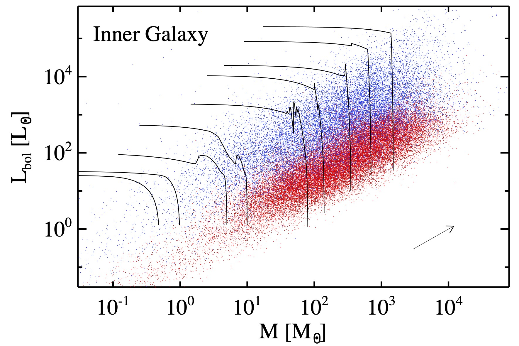
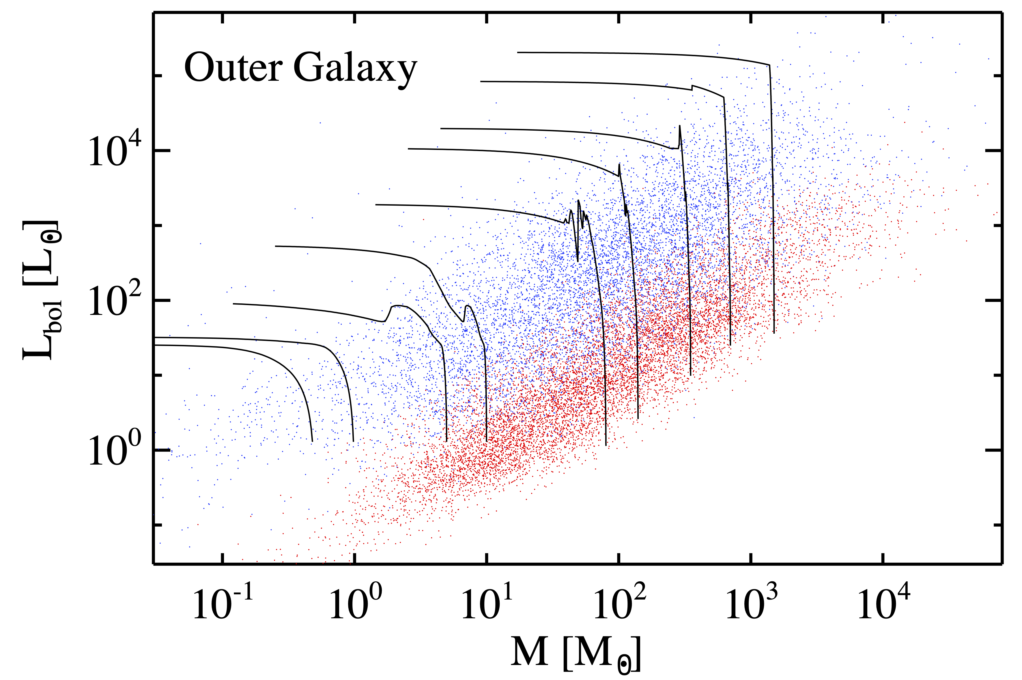
Figure 12: Top panel: bolometric luminosity vs envelope mass for pre-stellar (red) and protostellar (blue) sources in the inner Galaxy. The black lines represent evolution, upwards and then to the left, on tracks from Molinari et al. (2008). As in Fig. 10, since the distance estimate is the main source of uncertainty for both $M$ and $L_{\mathrm{bol}}$, a hypothetical distance increase of a factor 2 is represented as an arrow at the bottom right corner. Bottom panel: same as top panel, but for the outer Galaxy.

The $L_{\mathrm{bol}}$ vs $M$ diagram for the outer Galaxy sources (Fig. 12, bottom) exhibits qualitatively similar behaviour, but spans different ranges in mass and luminosity, most of which remain below $10^{3}~{}M_{\odot}$ and $10^{3}~{}L_{\odot}$, respectively. A different range for masses in the outer Galaxy, which can be explained only partially by different distances involved, has been discussed in Section 3.3. Similarly, here we use median luminosities calculated in bins of distance (Fig. 13) to show that like for masses, on average luminosities are also intrinsically lower in the outer Galaxy than in the inner Galaxy.

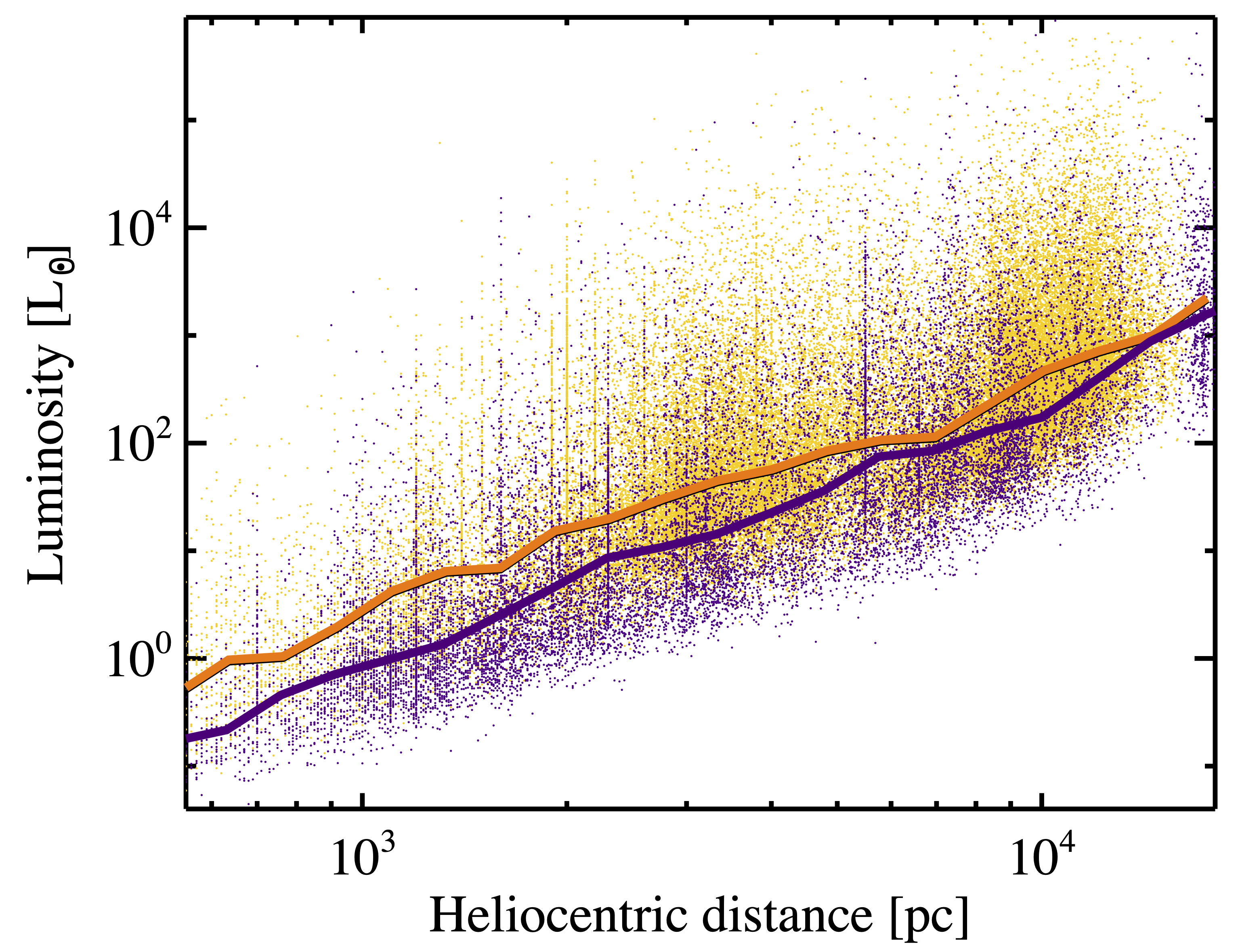
Figure 13: Same as Fig. 9, but for bolometric luminosity.

3.5 Clump lifetimes

Information about the bolometric luminosity might be used, in principle, to infer clump lifetimes similarly to Urquhart et al. (2018). They establish a relation between the H ii region lifetime $t_{\textrm{HII}}$ and the luminosity of their sources through the function $\log(t_{\textrm{HII}}/\textrm{yr})=(-0.13\pm 0.16)\times\log(L/L_{\odot})+(6.1\pm 0.8)$ of Mottram et al. (2011). A further link with the source mass is established, based on a mild $L_{\mathrm{bol}}$-$M$ power-law relation they recognise in their data. Finally, lifetimes of different evolutionary classes (quiescent, protostellar, young stellar objects, and massive star-forming regions, according to the classification of König et al., 2017) are derived as a function of mass bin by subdividing the total $t_{\textrm{HII}}(M)$ in proportion to the relative populations of these classes in each bin. In other words, the H ii region lifetimes are required to convert relative lifetimes, typically obtained from population ratios (cf., e.g., Battersby et al., 2017), to absolute ones.

Our approach contains some slight differences. First, we prefer not to identify a trend in the $L_{\mathrm{bol}}$-$M$ relation, given the high degree of degeneracy seen in Fig. 12. In Paper I a conservative threshold of $22.4~{}L_{\odot}/M_{\odot}$ was established to identify, in the absence of radio observations, a robust sub-sample of protostellar sources that are candidates to host an H ii region. This threshold was based on the $L_{\mathrm{bol}}/M$ distribution of Hi-GAL counterparts of CORNISH (Hoare et al., 2012; Purcell et al., 2013) radio sources obtained by Cesaroni et al. (2015). We prefer to insert that single-valued threshold in the aforementioned function of Mottram et al. (2011) to establish the relation between mass and the corresponding $t_{\textrm{HII}}$. The estimated lifetimes for the H ii regions are quite uncertain due to the error bars in the function of Mottram et al. (2011) and our choice of a constant value, $22.4~{}L_{\odot}/M_{\odot}$, as representative of this evolutionary stage. Second, we want to take into account differences among sources in terms of size (see discussion in Section 3.2) and thus underlying unresolved structure, which depends in turn on the heliocentric distance. Note also that in this analysis we do not include unbound clumps in general or all starless clumps in the low-reliability catalogue.

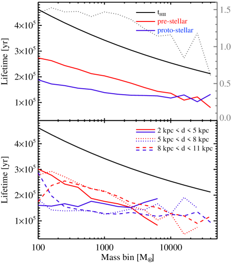
Figure 14: Lifetimes vs mass. The black line in each panel represents the mass dependence of the lifetime $t_{\textrm{HII}}$ for a clump hosting an H ii region according to $\log(t_{\textrm{HII}}/\textrm{yr})=-0.13\times\log(L/L_{\odot})+6.1$ (Mottram et al., 2011) and assuming $L_{\mathrm{bol}}/M=22.4~{}L_{\odot}/M_{\odot}$. By definition $t_{\textrm{HII}}$ is the sum of the lifetimes of the pre-stellar and protostellar phases, and so these lifetimes can be derived from the relative populations of these phases in each bin of mass (see the text). The numeric ratio of pre-stellar to protostellar clumps is also plotted as a dotted grey line, referring to the grey $y$-axis on the right. Top: lifetimes of pre-stellar (red line) and protostellar (blue line) clumps for the entire sample. Bottom: same as the top, but dividing the clumps into three different ranges of heliocentric distance: 2-5 kpc (solid lines), 5-8 kpc (dotted lines), and 8-11 kpc (dashed lines).

In Fig. 14 the results of this analysis are shown for the whole sample (upper panel) and for three different ranges of distances, 2-5, 5-8, and 8-11 kpc (lower panel). Unlike Urquhart et al. (2018), in our case quiescent pre-stellar sources represent the majority of the sample and this translates into a longer lifetime compared to that of protostellar clumps, for masses up to $\gtrsim 10^{4}~{}M_{\odot}$. The lower panel of the figure, however, shows how quantitatively different the relative behaviour of these two lifetimes becomes if a smaller range of distances, and hence masses, is considered. At closer distances, i.e., in the case less biased by distance, the behaviour is not unlike that seen overall, but the two curves cross at $M\sim 2\times 10^{3}~{}M_{\odot}$. The next case, from 5 to 8 kpc, is also similar to the overall curves, but there is a relative deficit of pre-stellar sources at low masses ($M\sim 100~{}M{\odot}$) and exaggerated change at the highest $M$. For the most distant case, 8-11 kpc, the deficit at low $M$ is much more pronounced so that the curves cross at $M\sim 140~{}M_{\odot}$. These differences serve as a caution that objects with the same mass but having a large range of distances might correspond to different kinds of structures, requiring separate analysis and conclusions.

Two further comments to this analysis are required. First, the constant $L_{\mathrm{bol}}/M$ ratio assumed for calculating H ii region lifetimes was determined in origin as a very conservative threshold. Adopting a reasonably lower value for it (for example, by a factor $\sim 2$, cf. Cesaroni et al., 2015) would imply, for a fixed mass bin, to linearly decrease also the luminosity appearing in the reported relation by Mottram et al. (2011) and, consequently, to estimate a systematically longer lifetime.

Second, it is to notice that the analysis above would remain qualitatively identical, in terms of relative proportions of pre-stellar and protostellar sources in single mass bins, if another set of total lifetimes was adopted to absolutely scale the clump lifetimes. For example, while here we used H ii region lifetimes similarly to Urquhart et al. (2018), Svoboda et al. (2016) used lifetimes of CH₃OH masers, and Battersby et al. (2017) used both. Considering only the behaviour of the class mutual proportions, we see that in our case the pre-stellar to protostellar ratio decreases at increasing mass bin (Fig. 14, top) as in Svoboda et al. (2016), but with a shallower slope, essentially in the range between $10^{2}$ and $10^{3}~{}M_{\odot}$. This is due to a relevant amount of pre-stellar clumps also at relatively large masses for which, in turn, two explanations can be given: $i$) the larger fraction of pre-stellar sources in the Hi-GAL catalogue compared to the BGPS case, and $ii$) the lower temperatures obtained for many Hi-GAL pre-stellar clumps from MBB fit, compared with the kinetic ones adopted by Svoboda et al. (2016), which typically imply higher masses. Interestingly, the pre-stellar to protostellar number ratio of $\sim 1.5$ observed in Fig. 14 for masses up to $\sim 10^{3}~{}M_{\odot}$ corresponds to a relative time of 60 per cent spent in the pre-stellar phase and 40 per cent in the protostellar, which is consistent with an analogous estimate of Battersby et al. (2017). For the population ratio of $\sim 1.2$ achieved at $10^{4}~{}M_{\odot}$ (over this value the curve starts to show significant scatter), the above time fractions change to 55 per cent and 45 per cent, respectively. Notice that, for consistency with Svoboda et al. (2016) and Battersby et al. (2017) papers, the above comparisons have been made by considering our entire sample, with no division in distance bins as done for Fig. 14, bottom.

4 Distance-independent parameters

Given the large uncertainties existing on heliocentric distance estimates (Mège et al., accepted), the analysis of distance-independent source parameters is surely more robust, being formally unbiased. Actually, distance affects the meaning that we can assign to such observables, because they are single global/average numbers describing entire complex but unresolved structures. For example, a fundamental difference exists between assigning an average temperature to a protostellar core and to a much larger clump, in which a wider variety of physical conditions can coexist, from active star-forming sites to quiescent regions. Notwithstanding, the analyses by Baldeschi et al. (2017a); Baldeschi et al. (2017b) on how the distance bias affects temperature and the luminosity/mass ratio, respectively, suggest that, in general, global estimates of these parameters for distant clumps mirror the average behaviour for the same parameters in the underlying population of cores. This encourages us to discuss distance-independent parameters and to propose evolutionary classification metrics based on them (Section 4.6).

4.1 Luminosity-mass ratio

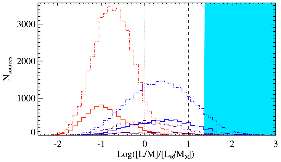
Figure 15: Distributions of the ratio of bolometric luminosity to envelope mass for pre-stellar (red histograms), protostellar (blue histograms) and MIR-dark protostellar (dark purple histograms, arbitrarily enhanced by a factor of 2 to improve the readability) Hi-GAL sources considered for science analysis in this paper. Dot-dashed histograms are for the inner Galaxy and solid for the outer. The dotted and the dashed vertical lines represent the thresholds identified by Molinari et al. (2016b) for expecting star formation to be traced by line emission of methyl-acetylene CH₃C₂H(12-11) or by the presence of a zero age main sequence (ZAMS) star inside the clump, respectively. The light blue-shaded area contains clumps that are candidates to host H ii regions (see the text).

We discuss first the ratio of bolometric luminosity to envelope mass, $L_{\mathrm{bol}}/M$. As we will see below, a threshold on this parameter allows us to identify a sub-class of particularly evolved protostellar sources, to be analysed subsequently in light of the additional distance-independent quantities.

Figure 15 shows the distribution of this ratio for both the pre-stellar and protostellar sources, in both the inner and outer Galaxy. A good degree of segregation is seen between the two classes of objects, especially in the outer Galaxy. We evaluate its extent by quantifying the fraction of the histogram area of a source class overlapping the histogram of the other class, and vice versa, as follows: given two generic histograms $H_{1}$ and $H_{2}$ defined over the same $N_{\mathrm{bin}}$ bins, the area of their overlap region is $\sum_{i=1}^{N_{\mathrm{bin}}}\min(H_{1}(i),H_{2}(i))$. The overlap fractions for the two histograms are this number divided by the integral of $H_{1}$ and $H_{2}$, respectively. For the adopted histogram bin size of Fig. 15 (0.1 for $\log_{10}([L_{\mathrm{bol}}/M]/[L_{\odot}/M_{\odot}])$), for the inner Galaxy the overlap fractions are 27 per cent for pre-stellar sources and 39 per cent for protostellar sources. For the outer Galaxy they drop to 25 per cent and 29 per cent, respectively, i.e., more segregation.

Correspondingly, a larger gap between median values is observed in the outer Galaxy: medians of $L_{\mathrm{bol}}/M$ for pre-stellar and protostellar sources are 0.2 $L_{\odot}/M_{\odot}$ and 2.6 $L_{\odot}/M_{\odot}$, respectively, in the inner Galaxy, and 0.1 $L_{\odot}/M_{\odot}$ and 3.1 $L_{\odot}/M_{\odot}$, respectively, in the outer Galaxy.

All four values are lower than $10~{}L_{\odot}/M_{\odot}$, around which the ATLASGAL sources of Urquhart et al. (2018) appear to have a concentration. But these are among the brightest far-infrared sources in the Galaxy and Hi-GAL, which is remarkably more sensitive, is able to detect significantly fainter sources. Table 4 records these medians along with medians of all distance-independent parameters, separately for different evolutionary classes and inner/outer Galaxy location.

Table 4: Median values for distance-independent physical parameters, subdivided by evolutionary class and sub-class and inner/outer Galaxy location.

	Inner Galaxy					Outer Galaxy
	Pre-stellar	Protostellar				Pre-stellar	Protostellar
		All	MIR-dark	Hii candidates			All	MIR-dark	Hii candidates
$L_{\mathrm{bol}}/M\,[L_{\odot}/M_{\odot}]$	0.2	2.6	1.2	40.4		0.1	3.1	1.7	39.7
$T$  [K]	11.4	15.2	14.6	24.6		10.5	15.3	15.3	23.9
$L_{\mathrm{bol}}/L_{\mathrm{smm}}$	5.7	30.4	15.6	191.9		4.4	36.9	30.9	199.6
$T_{\mathrm{bol}}$  [K]	17.6	39.5	23.7	50.5		16.2	43.4	25.6	51.5
$\Sigma$  [g cm-2]	0.14	0.21	0.24	0.07		0.10	0.12	0.15	0.05

The uncertainty of each median can be estimated as $(Q_{3}-Q_{1})/(2\sqrt{N_{\mathrm{tot}}})$, i.e., as the half distance between the third and the first quartile of the distribution (also a surrogate for the standard deviation in the case of strongly asymmetrical distributions), divided by the square root of the total number of counted objects, which can be quite different for different populations (Table 1). Consequently, the uncertainty of the median of $L_{\mathrm{bol}}/M$ ranges from $0.001~{}L_{\odot}/M_{\odot}$ for pre-stellar sources in the inner Galaxy to $0.6~{}L_{\odot}/M_{\odot}$ for Hii region candidates in the outer Galaxy. Similarly, uncertainties of the median range from 0.007 to 0.1 K for $T$, from 0.01 to 2 for $L_{\mathrm{bol}}/L_{\mathrm{smm}}$, from 0.01 to 0.02 K for $T_{\mathrm{bol}}$, and from 0.0005 to 0.001 g cm^-2 for $\Sigma$.

Detection of CH₃C₂H(12-11) line emission is considered a signature of ongoing star formation. By cross-correlation, Molinari et al. (2016b) proposed a threshold of 1 $L_{\odot}/M_{\odot}$ for detection. Fig. 15 shows that in the inner Galaxy this threshold falls well inside the region of the pre-stellar/protostellar overlap, whereas in the outer Galaxy only a small fraction of pre-stellar clumps is found above this threshold. As seen by Zhang et al. (2020), quiescent massive clumps associated with H ii regions can reach $L_{\mathrm{bol}}/M>10~{}L_{\odot}/M_{\odot}$ because of significant external heating, suggesting a more advanced evolutionary state than is the case. The higher density of H ii regions in the inner Galaxy compared to the outer Galaxy (Anderson et al., 2014) and, in general, the stronger interstellar radiation field (e.g., Mathis et al., 1983) can create the higher degree of overlap in the inner Galaxy. Thus, this effect is probably the major cause of the overlap of the pre-stellar distribution into the protostellar distribution, for this parameter and also the others discussed in the following sections. A further check to address this is described in Section 4.6.

Additional contamination between the two classes can arise from source misclassification due to the aforementioned distance bias, as examined in Paper I. This is expected to be more of an issue in the inner Galaxy because of the larger heliocentric distances ($d>12$ kpc) there.

Molinari et al. (2016b) further proposed a threshold of 10 $L_{\odot}/M_{\odot}$ at which the temperature derived from CH₃C₂H(12-11) starts to increase monotonically for increasing $L_{\mathrm{bol}}/M$, and interpreted this as the appearance of one or more ZAMS stars in the clump. In our data for both the inner and the outer Galaxy a significant fraction of protostellar sources is found beyond this value (21 per cent and 24 per cent, respectively), whereas the presence there of pre-stellar sources is negligible.

The light blue shaded area in Fig. 15 corresponds to the $22.4~{}L_{\odot}/M_{\odot}$ threshold for identifying candidate H ii regions, as introduced in textbfSection 3.5 (see also Elia, 2020). We find 2806 candidates in the inner Galaxy and 869 in the outer Galaxy. These are expected to be the most evolved sources in our catalogue. Their corresponding median values are reported in Table 4. Checking for further evidence of the H ii region nature of these objects is not among the aims of this paper. Nevertheless, we cross-matched the positions of these sources with the WISE catalogue of H ii regions by Anderson et al. (2014) and found 2560 matches, 2192 of which are associated with regions showing radio emission.

On the opposite side of the distribution for the protostellar class we expect to find the MIR-dark sources (cf. Paper I, ), i.e., those having a detection at $70~{}\mu$m but no detection at shorter wavelengths (MSX/WISE/MIPSGAL). However, as already shown in Paper I, although evolutionary parameters of these sources do indicate, on average, an earlier stage with respect to the global population of protostellar sources, they do not actually produce a clear “left tail” of the protostellar distribution. This is confirmed by the distributions plotted for this sub-class in Fig. 15, which extend over a wide range of $L_{\mathrm{bol}}/M$ values both in the inner and in the outer Galaxy. Their corresponding median values are reported in Table 4.

4.2 MBB temperature

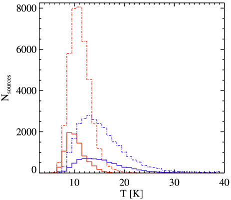
Figure 16: Distributions of MBB temperature for pre-stellar (red histograms) and protostellar (blue histograms) sources. Dot-dashed histograms are for the inner Galaxy and solid for the outer.

In Paper I it has been demonstrated that the dust temperature $T$ estimated by the MBB fit of SEDs at $\lambda\geq 160~{}\mu$m shows quite different distributions for pre-stellar and protostellar sources. Moreover, temperature itself is a reliable evolutionary parameter for protostellar sources. It is reasonably well correlated with other evolutionary indicators, first of all $L_{\mathrm{bol}}/M$, although it produces a lower degree of segregation.

These conclusions are corroborated by the extension of our analysis to the outer Galaxy. In Fig. 16 the new temperature distributions for both pre-stellar and protostellar sources in the outer Galaxy are shown, together with those in the inner Galaxy for comparison. It is confirmed that also in the outer Galaxy the temperature of protostellar sources is higher, on average, than that of pre-stellar sources, as it was already found for the inner Galaxy in Paper I and also in Svoboda et al. (2016) and Merello et al. (2019), based on independent ammonia observations. Similarly to the behaviour seen for $L_{\mathrm{bol}}/M$ in Section 4.1, a higher degree of segregation between the two distributions is found in the outer Galaxy, probably due to a lower impact of the environment on the temperature of pre-stellar clumps (see Section 4.6). Using the same method to determine the overlap of the two pre-stellar and protostellar histograms, we find that in the outer Galaxy the overlap fraction corresponds to 39 per cent and 44 per cent, respectively, compared with 39 per cent and 57 per cent, respectively, in the inner Galaxy. Correspondingly, the median values of $T$ are also found to be more distant from each other in the outer Galaxy (10.5 K and 15.3 K for pre-stellar and protostellar population, respectively), than in the inner Galaxy (11.4 K and 15.2 K, respectively). See again Table 4. Notice that, despite the degree of overlap between pre-stellar and protostellar distributions, the gap between their medians is meaningful, being even broader than similar estimates: Liu et al. (2018) found 13.5 K and 15.5 K, respectively, in a sample of MALT90 (Jackson et al., 2013) clumps with Hi-GAL counterparts.

Here we briefly discuss whether and how the observed segregation among source classes (and sub-classes) in Fig. 16 can be affected by our choice of using a single and common opacity law for the MBB fit of all SEDs in the catalogue. Indeed, variations of the $\beta$ exponent are observed in the ISM (e.g., Sadavoy et al., 2016), and generally interpreted as a consequence of dust grain evolution. Neglecting for a moment other dust parameters, it can be roughly said that grain growth produces a decrease of $\beta$ (e.g., Beckwith & Sargent, 1991; Guzmán et al., 2015; Merello et al., 2015; Li et al., 2017). In our case, to possibly consider a smaller value of $\beta$ for protostellar sources with respect to pre-stellar sources would imply an increase of the temperature estimated through the MBB fit (Désert et al., 2008; Martin et al., 2012), and consequently a higher level of separation in Figure 16 between the distributions of these two classes. However grain growth is observed to occur mostly in the vicinity of forming stars, then its most relevant effects can be observed mainly in resolved cores located in nearby regions as those studied by Sadavoy et al. (2016). This discourages us to consider a differentiation of $\beta$, rather than a common value, for Hi-GAL clump SEDs, which are dominated by the emission of the large-scale envelope.

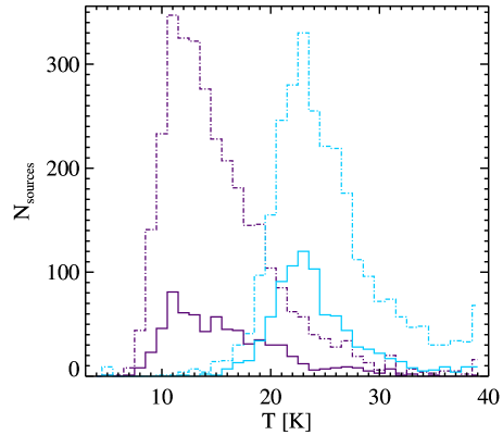
Figure 17: Same as Fig. 16, but for two particular sub-classes of the protostellar sample: MIR-dark sources (dark purple histograms) and H ii region candidates (light blue histograms).

To explore in more detail the temperatures of sub-classes of the protostellar sample, namely MIR-dark and candidate H ii regions, we plot separately their temperature histograms in Fig. 17. As expected, candidate H ii regions are found at relatively high temperatures.

The median temperatures of candidate H ii regions in the inner and outer Galaxy are 24.6 K and 23.9 K, respectively, but both distributions are right-skewed and the 10th percentiles are at 20.4 K and 20.3 K, respectively. Liu et al. (2018), Guzmán et al. (2015), and Urquhart et al. (2013b) estimated a typical temperature of 22.5 K, 23.7 K and 25.0 K, respectively, for clumps hosting an ultra-compact H ii region, which is in good agreement with our statistics. Based on Hi-GAL data for twelve known H ii regions, Paradis et al. (2014) found temperatures in the range 22-45 K. However, they included the $70~{}\mu$m data in their fits, both a simple MBB and a more refined model for dust grain emissivity, then accounted for measurements from a warmer dust component. Similarly, but considering only $\lambda>70~{}\mu$m, Paladini et al. (2012) found temperatures in the range 20-30 K for Hi-GAL counterparts of a sample of 16 evolved H ii regions. Finally, although again with a small sample of eight resolved H ii regions observed in HOBYS survey (Motte et al., 2010), Anderson et al. (2012) highlighted that a fit to their entire SED yields, on average, a temperature of about $25$ K, but that considering their internal components individually average temperatures range from about $15$ K for infrared dark clouds to $26$ K for photodissociation regions. The compatibility of these previous values with median temperatures obtained for our H ii region candidates supports the reliability of the identification criterion established in Section 4.1.

The MIR-dark sub-class is expected to be less evolved among the protostellar sources and indeed the median values of $T$ are relatively low (14.6 K in the inner Galaxy and 15.3 K in the outer). However, the distributions in Fig. 17 show a significant range and are skewed towards higher temperatures, even overlapping the distributions for the H ii region candidates. This behaviour, already highlighted in Paper I, is found also for the outer Galaxy.

4.3 Ratio of bolometric to submillimetre luminosity

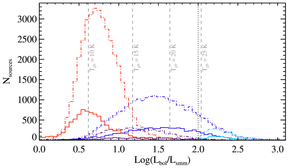
Figure 18: Distributions of the ratio of the bolometric luminosity to the portion in the sub-millimetre ($\lambda\geq 350~{}\mu$m) for the pre-stellar (red histograms), protostellar (blue histograms), MIR-dark protostellar (dark purple histograms, arbitrarily enhanced by a factor of 2 to improve the readability), and H ii-region candidate (light blue histograms) Hi-GAL sources, respectively. Dot-dashed histograms are for the inner Galaxy and solid for the outer. For a MBB with $\beta=2$, the dashed grey vertical lines mark ratios corresponding to the different MBB temperatures indicated. The dotted black line at $L_{\mathrm{bol}}/L_{\mathrm{smm}}=100$ marks the ratio separating Class 0 from Class I low-mass YSOs as proposed by Maury et al. (2011).

We also use the ratio of the bolometric luminosity $L_{\mathrm{bol}}$ to the portion $L_{\mathrm{smm}}$ in the sub-millimetre ($\lambda\geq 350~{}\mu$m) as an evolutionary indicator. This was introduced by André et al. (2000) for discriminating between Class 0 and Class I young stellar objects (YSOs) in the low-mass star formation regime (with a separation threshold fixed at $L_{\mathrm{bol}}/L_{\mathrm{smm}}=100$, Maury et al., 2011), but here it cannot be used for such a classification because the sources being discussed are clumps containing entire star-forming regions, possibly including high-mass star formation. Nevertheless, as seen in Paper I, this parameter remains interesting because it also ensures a good segregation among the evolutionary classes proposed for our sources.

The distributions of $L_{\mathrm{bol}}/L_{\mathrm{smm}}$ for the inner and the outer Galaxy can be compared in Fig. 18. Similar to parameters analysed in previous sections, we note a stronger segregation between pre-stellar and protostellar populations in the outer Galaxy, than in the inner Galaxy. This is quantified by the lower overlap fractions (21 per cent for pre-stellar sources and 24 per cent for protostellar sources in the outer Galaxy, against 22 per cent and 32 per cent, respectively, in the inner Galaxy), and by a larger gap between median values of the two populations (4.4 and 36.9 in the outer Galaxy, respectively, against 5.7 and 30.4 in the inner Galaxy). See again Table 4.

The values expected for a MBB (cf. Elia & Pezzuto, 2016) with $\beta=2$ are shown for four temperatures $T=10,~{}15,~{}20,~{}25$ K in Fig. 18, along with the aforementioned $L_{\mathrm{bol}}/L_{\mathrm{smm}}=100$ (close to the one for $T=25$ K). We notice that almost all the H ii region candidates lie above 100, suggesting this threshold as a necessary condition in searching for H ii region candidates among protostellar clumps.

4.4 Bolometric temperature

The bolometric temperature $T_{\mathrm{bol}}$ has been found by Paper I to be the parameter for which the segregation between pre-stellar and protostellar sources is highest. It is defined as the average frequency of the SED, weighted with fluxes, and translated in terms of temperature of an equivalent blackbody (Myers & Ladd, 1993). For an analytic MBB, the relation between $T_{\mathrm{bol}}$ and the MBB temperature is linear (e.g. Elia & Pezzuto, 2016). However, here the MBB temperature is determined for data at $\lambda\geq 160~{}\mu$m and so for sources with data at $\lambda<100~{}\mu$m in excess of the fitted MBB, $T_{\mathrm{bol}}$ is necessarily higher than in the linear relation, being particularly sensitive to MIR fluxes where detected (the impact of failure to detect a faint MIR counterpart near the survey sensitivity limit on the estimate of $T_{\mathrm{bol}}$ is discussed in Appendix B).

As for other evolutionary indicators, the distributions of $T_{\mathrm{bol}}$ for pre-stellar and protostellar sources in the outer Galaxy appear better separated than in the inner Galaxy (Fig. 19). In the outer Galaxy, overlap fractions for the two histograms are 5 per cent and 5 per cent for pre-stellar and protostellar clumps, respectively, and median values are 16.2 K and 43.4 K, respectively, whereas in the inner Galaxy these quantities are 9 per cent and 14 per cent, and 17.6 K and 39.5 K.

Figure 19: Distributions of bolometric temperature for pre-stellar (red) and protostellar (blue) sources. Dot-dashed histograms are for the inner Galaxy and solid for the outer.

We can extend to the outer Galaxy two general considerations expressed in Paper I concerning the inner Galaxy. First, almost all sources have $T_{\mathrm{bol}}<70$ K, which was recognised as the threshold between Class 0 and Class I objects by Chen et al. (1995) in the low-mass star formation regime. Second, values we find are smaller than those of Mueller et al. (2002) and Ma et al. (2013), who considered SEDs more dominated by MIR fluxes.

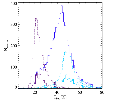
Figure 20: Same as Fig. 19, but for MIR-dark sources (dark purple) and H ii region candidates (light blue). In addition, the distribution for all protostellar sources in the outer Galaxy (solid blue, also shown in Fig. 19) is given for comparison.

The distributions of $T_{\mathrm{bol}}$ for both MIR-dark and H ii region candidates are reported separately in Fig. 20. Unlike in the case of the MBB temperature (Fig. 17), here the two sub-classes appear well segregated. As already found in Paper I for inner Galaxy sources, the MIR-dark sources in the outer Galaxy also produce the left tail of the entire protostellar distribution, as expected from the definition of $T_{\mathrm{bol}}$. For H ii region candidates the distributions are shifted towards high $T_{\mathrm{bol}}$ (with median values 51.5 K and 50.5 K in the outer and in the inner Galaxy, respectively); however, they make up only a subset of the right tail of the entire protostellar distribution.

4.5 Surface density

The surface density parameter $\Sigma$ summarises the mass-radius relation studied in Section 3.3. Distributions of $\Sigma$ are shown in Fig. 21. Unlike for the other parameters, the segregation of pre-stellar and protostellar sources is not obvious.

In Paper I we highlighted an increase of median surface density from pre-stellar to protostellar sources (see also Battersby et al., 2014). Furthermore, the median surface density of MIR-dark sub-sample was even higher, suggesting that the highest density is achieved around this stage, before the source starts to emit in the MIR. At later times, stellar feedback can start to be relevant in producing envelope dissipation and so a possible decrease of median surface density. The effect of this evolution should be most evident on the opposite side of protostellar class, i.e., for H ii region candidates (cf. Guzmán et al., 2015), though this is complicated by the very large spread in that distribution around the median (cf. also Fehér et al., 2017).

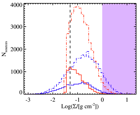
Figure 21: Distributions of surface density for pre-stellar (red histograms) and protostellar (blue histograms) in the inner Galaxy (dot-dashed histograms) and the outer (solid histograms). The zone surpassing the Krumholz & McKee (2008) threshold of 1 g cm^-2 is shaded purple, as in Fig. 10. The lowest surface density at which massive star formation is found by Urquhart et al. (2014), namely $\Sigma=0.05$ g cm^-2, is also reported as a dotted vertical line. Other thresholds for compatibility with massive star formation, discussed in Section 3.3, cannot be represented in this plot because they do not correspond to a constant value of $\Sigma$.

This trend of median surface densities in the inner Galaxy is confirmed in this work, with values 0.14, 0.24, 0.21, and 0.07 g cm^-2 for pre-stellar, MIR-dark, protostellar, and H ii region candidates, respectively (Table 4). In the outer Galaxy the sequence is 0.10, 0.15, 0.12, and 0.05 g cm^-2. Although the trend is the same, the median surface densities are systematically lower for all classes, as can be appreciated also in Figs. 21 and 22 (cf. also Zahorecz et al., 2016). This is connected directly to the different regimes of masses observed in the inner and outer Galaxy (Fig. 9).

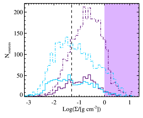
Figure 22: Same as Fig. 21, but for two sub-classes of the protostellar sample: MIR-dark sources (dark purple histograms) and H ii region candidates (light blue histograms).

To connect this information in a more systematic way, the surface density is discussed again in Section 5 as a function of the Galactocentric radius.

4.6 Overall classification

Figure 23: Radar plot for the median values of five distance-independent physical parameters (see text) for pre-stellar clumps, for the inner Galaxy (dot-dashed line) and the outer (solid line). Scales on each axis are linear, ranging from 0 to the value specified at the end.

To give a synoptic view of median values of the distance-independent observables discussed in previous sections, we adopt the radar chart visualisation of $L_{\mathrm{bol}}/M$, $T$, $\Sigma$, $T_{\mathrm{bol}}$, and $L_{\mathrm{bol}}/L_{\mathrm{smm}}$ as introduced in Paper I. Five axes represent these parameters on the linear scales indicated. The median values are plotted on each axis and connected by lines between adjacent axes to form a polygon. Medians taken for different source sub-samples, whether selected by classification and/or distances, are displayed in the same plot for the purpose of comparison.

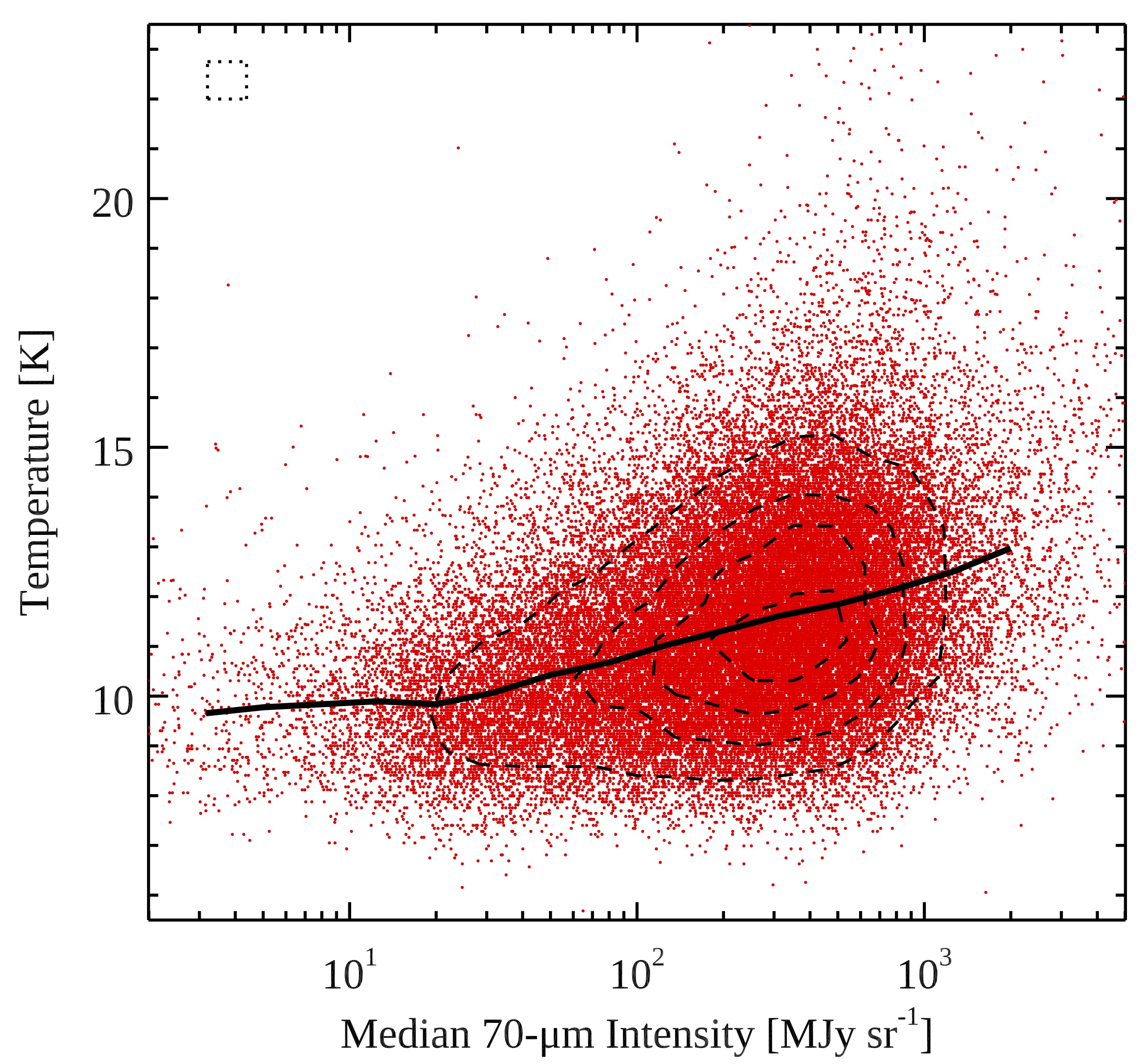
Figure 24: Temperature $T$ of pre-stellar sources vs median intensity $\bar{I}_{70}$ evaluated in $61\times 61$ pixel boxes centered on clump centroids in PACS 70 $\mu$m maps. For clarity, the density of points in the plot, evaluated on a grid whose element has the size of the dotted box placed at the top left corner of the plot, is represented with dashed contours starting from 200 and in steps of 200.

Medians of $T$ in bins of $\log\bar{I}_{70}$ (bin width = 0.2) are connected by the solid line.

The first such plot is Fig. 23 representing median values for pre-stellar sources, for inner and outer Galaxy separately. All medians, and in particular the four evolutionary indicators $L_{\mathrm{bol}}/M$, $T$, $T_{\mathrm{bol}}$, and $L_{\mathrm{bol}}/L_{\mathrm{smm}}$, are larger in the inner Galaxy, as already seen in Sections 4.1-4.5. A hasty interpretation might be that pre-stellar clumps in the inner Galaxy are “more evolved” on average. However, it is more plausible to ascribe this to different environmental conditions in the inner and outer Galaxy, because external irradiation (Mezger, 1990, and references therein) is the main source of heating for pre-stellar clumps (e.g., Evans et al., 2001; Lippok et al., 2016; Yuan et al., 2017; Merello et al., 2019).

To assess the effects of external heating, it is sufficient to analyse the pre-stellar clump temperature as a function of the Galactic position, because for a MBB (as pre-stellar SEDs are expected to follow) the $L_{\mathrm{bol}}/M$, $L_{\mathrm{bol}}/L_{\mathrm{smm}}$, and $T_{\mathrm{bol}}$ quantities are expected to increase monotonically with increasing temperature, following precise analytic relations (Elia & Pezzuto, 2016). As a proxy for the interstellar radiation field (Compiègne et al., 2010; Bernard et al., 2010), we used the intensity of $70~{}\mu$m emission in the neighbourhoods of clumps: for each clump we found the average, $\bar{I}_{70}$, of the PACS $70~{}\mu$m intensity over a $61\times 61$ pixel ($\sim 3.25\times 3.25$ arcmin²) sub-frame centered on the source centroid (or smaller, if limited by proximity to tile border). We first explored the relationship of $\bar{I}_{70}$ to source temperature (Fig. 24). Due to the relatively narrow temperature distribution of pre-stellar clumps seen in Fig. 16, we do not expect large variations of the temperature as a function of $\bar{I}_{70}$. Furthermore, we also do not expect a straightforward relation between these two observables in all cases, because environmental conditions can change locally. However, considering the entire sample in Fig. 24 the median temperature in bins of $\bar{I}_{70}$ is seen to increase at increasing $\bar{I}_{70}$.

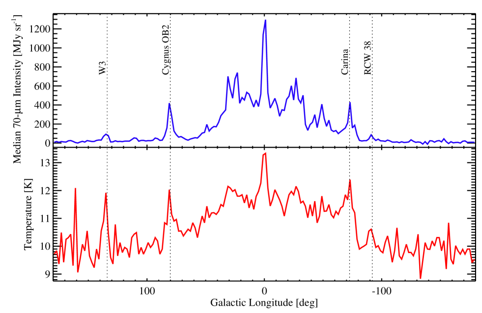
Figure 25: Medians, in $2^{\circ}$-bins of Galactic longitude, of two quantities characterizing pre-stellar sources. Upper panel: median intensity $\bar{I}_{70}$ of the $70~{}\mu$m map intensity around pre-stellar sources (see Fig. 24). Lower panel: source temperature. Dashed vertical lines indicating the average longitudes of the labelled star-forming clouds in the outer Galaxy are coincident with local peaks in the curves in both panels.

Fig. 25 shows the behaviour of $T$ and $\bar{I}_{70}$ individually as a function of Galactic longitude. In the central quadrants $\bar{I}_{70}$ is far more intense and the median $T$ of pre-stellar sources increases correspondingly. Furthermore, main local peaks of the two quantities spatially coincide (cases of average longitudes of Cygnus OB2, W3, RCW 38, and Carina star-forming clouds). These correlations can not be simply casual, even if the variability range of median $T$ in the bottom panel of Fig. 25 might appear relatively narrow. It should be considered, indeed, that the response of dust temperature to the ultraviolet field is expected by Bernard et al. (2010) to follow a power law with an exponent as shallow as $1/(4+\beta)$.

Because a fraction of outer Galaxy sources can be found at relatively low $|\ell|$, the observed decrease of pre-stellar source temperature has to be confirmed, more rigorously, as a function of Galactocentric distance. This will be shown in Section 5. We can conclude that the general increase of temperature and other evolutionary parameters for pre-stellar clumps in the inner Galaxy is related mostly to the amount of irradiation to which they are exposed.

Figure 26: Same as Fig. 23, but for protostellar sources.

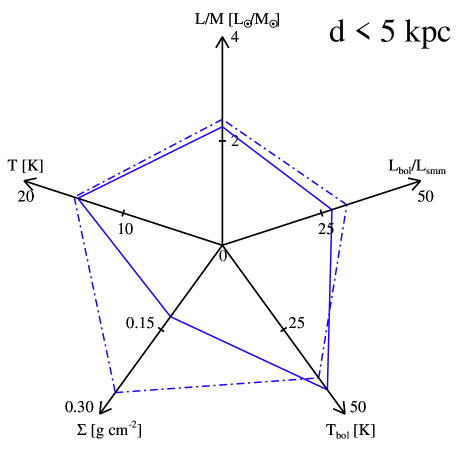
Figure 27: Same as Fig. 26, but for the sub-set of protostellar sources within heliocentric distance $d<5$ kpc.

An opposite trend is shown by statistics of protostellar sources in Fig. 26: the medians of $T$ have become about equal and the medians of the other three evolutionary indicators are now higher in the outer Galaxy. For this class, because the main source of clump heating is internal, the influence of the environment is less relevant, and one could attribute a genuine evolutionary meaning to this behaviour. However, it is necessary to take into account possible basic systematic differences between the samples of protostellar clumps from the inner and outer Galaxy. The biggest factor is probably represented by the different distribution of heliocentric distances, highlighted by Fig. 5, because it produces a globally different distribution of physical sizes. The inner Galaxy contains a large number of sources located at $d>5$ kpc, which are unresolved structures of increasing complexity containing protostellar cores but also quiescent cores and inter-core medium (see Paper I, their Appendix C). This can affect some evolutionary indicators. To check this, in Fig. 27 we show a radar plot similar to that of Fig. 26, but limited to distances $d<5$ kpc. The largest effect is reductions of the medians of $L_{\mathrm{bol}}/M$ and $L_{\mathrm{bol}}/L_{\mathrm{smm}}$, making them along with the two median temperatures indistinguishable in the inner and outer Galaxy. We therefore conclude that the distance bias can significantly affect some source evolutionary indicators and consequently the classification too.

Like for the pre-stellar sources, the median $\Sigma$ for protostellar sources is higher in inner Galaxy. Limiting to the $d<5$ kpc sub-samples, the medians increases in both the inner and outer Galaxy, but more so for the inner so that their discrepancy increases. This can be explained with the intrinsically different regimes of density in the two zones, as already highlighted in Section 4.5 and further discussed, in terms of Galactocentric distance in Section 5.

5 Trends with the Galactocentric radius

In this section we move on from the inner-outer Galaxy dichotomy introduced in Section 2.2 to discuss all distance-independent parameters as a function of $R_{\mathrm{GC}}$, similarly to Paper I (their Section 8.2), but over a wider range of $R_{\mathrm{GC}}$ and also including pre-stellar clumps. Contrary to Section 4, the analysis presented here is based only on the statistics of sources with a known distance, as required to compute $R_{\mathrm{GC}}$. Fig. 28 shows the average behaviour of various parameters for different evolutionary classes.

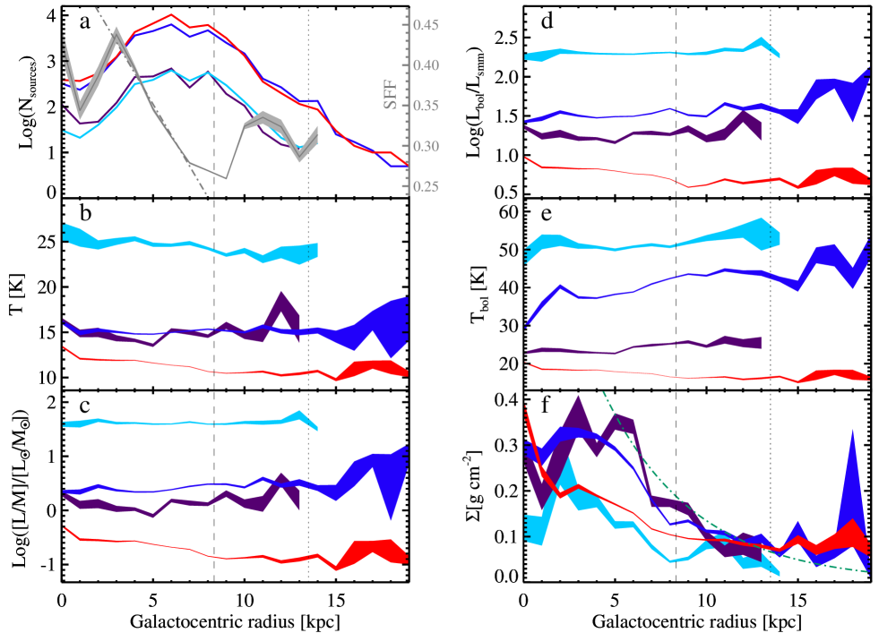
Figure 28: Characterization of sources vs Galactocentric radius in bins of 1 kpc for various populations: pre-stellar sources (red), all protostellar sources (blue), H ii-region candidates (light blue), and MIR-dark protostellar clumps (dark purple). The vertical dashed and dotted lines mark the values adopted for the Solar circle and inner radius of the far outer Galaxy, respectively. Panel $a$: number of sources. The star-forming fraction (SFF, see the text) is also plotted in grey, referring to the grey $y$-axis on the right. The grey dot-dashed line represents a fit to the SFF data in the range $3~{}\mathrm{kpc}\leq R_{\mathrm{GC}}\leq 7~{}\mathrm{kpc}$. The remaining panels $b$ through $f$ are for $T$, $L_{\mathrm{bol}}/M$, $L_{\mathrm{bol}}/L_{\mathrm{smm}}$, $T_{\textrm{bol}}$, and $\Sigma$, as labelled. In each bin the median and its uncertainty, calculated from interquartile ranges as explained in Table 4, are calculated and then the uncertainty intervals are displayed as shaded areas. Values are shown only for bins with at least 10 sources. In panel $f$, the green dot-dashed curve represents the radial dependence of the inverse of the gas-to-dust ratio predicted by Giannetti et al. (2017); the vertical scaling of the curve is arbitrary.

5.1 Number counts and star formation fraction

The source number in bins of Galactocentric radius is shown in panel $a$ to give an idea of the statistical relevance of curves shown in the subsequent panels. Unlike the bottom panel of Fig. 5, this does not separate between inner and outer Galaxy populations.

It also reports the curves corresponding to the two sub-classes of MIR-dark and candidate H ii regions, for which here we make some further considerations in addition to those in Section 3.1. The fraction of these two sub-classes with respect to the whole protostellar population is quite constant. The only exception is an excess of MIR-dark sources in the $R_{\mathrm{GC}}=0$ kpc bin, a bias produced by severe saturation affecting both the MIPSGAL and WISE-W4 band observations towards the Galactic centre. No MIR-dark sources are found at $R_{\mathrm{GC}}>14$ kpc and there are few of either major class in the far outer Galaxy (FOG). A local peak for H ii region candidates is found around 6 kpc, corresponding approximately to the enhancement of H ii regions found by Anderson & Bania (2009); however, this peak also coincides with local peaks of our pre-stellar and overall protostellar populations, with no particular excess there compared with other $R_{\mathrm{GC}}$. Therefore the local peak of H ii region candidates seems to be related to a global increased availability of molecular material near 6 kpc (Dobbs & Burkert, 2012) rather than to other specific conditions of the ISM.

Given the separate distributions of pre-stellar and protostellar sources with $R_{\mathrm{GC}}$, it is straightforward to investigate their fraction of the total. In particular, Ragan et al. (2016) discussed the “star-forming fraction” (hereafter SFF), namely the fraction of sources in the Hi-GAL catalogue of Paper I with a detection at 70 $\mu$m (i.e., the definition of protostellar source adopted here). Ragan et al. (2016) found a slightly decreasing behaviour of SFF over $3.1~{}\mathrm{kpc}<R_{\mathrm{GC}}<8.6~{}\mathrm{kpc}$, with a linear fit slope of $(-0.026\pm 0.002)$ kpc^-1. That analysis was carried out including all Hi-GAL sources with a known distance (including starless unbound). To enable comparison with Ragan et al. (2016), we have to consider sources in both of our catalogues, including unbound clumps.

The SFF curve obtained from our data, considering only 1-kpc bins containing at least 100 sources in total, is shown in panel $a$ of Fig. 28, referring to the $y$-axis on the right side. The behaviour of SFF is quite scattered, though confined to a relatively narrow range from 0.26 to 0.42. A decreasing trend is confirmed in the range $3~{}\mathrm{kpc}\leq R_{\mathrm{GC}}\leq 7~{}\mathrm{kpc}$, over which we derive a linear fit slope of $(-0.040\pm 0.003)~{}\mathrm{kpc}^{-1}$, similar to that of Ragan et al. (2016). However, embedded in a larger range of $R_{\mathrm{GC}}$, here such behaviour does not seem global anymore. Indeed, isolated increases of the fraction of protostellar sources are seen, due to local conditions, e.g., the Galactic centre position, around $R_{\mathrm{GC}}=3$ kpc (cf. Luna et al., 2006) and, in the outer Galaxy, 12 and 14 kpc, neither related to spiral arms (see Section 3.1) and possibly affected by relatively poor statistics. These fluctuations constitute a departure from a simple scenario in which the SFF, in turn related to star formation efficiency, decreases systematically from the centre to the periphery of Milky Way, which was considered already by Ragan et al. (2016) to be not easily explicable.

5.2 Evolutionary indicators

Looking at the behaviour of the evolutionary indicators $T$, $L_{\mathrm{bol}}/M$, $L_{\mathrm{bol}}/L_{\mathrm{smm}}$, and $T_{\mathrm{bol}}$ in panels $b$ to $e$, respectively, first of all we notice that for each parameter the degree of segregation among classes/sub-classes and their ranking is preserved across the range of $R_{\mathrm{GC}}$ explored. For example, as seen in Section 4, the average temperatures of MIR-dark sources are not distinguishable from those of the global protostellar population, while other indicators, especially $L_{\mathrm{bol}}/L_{\mathrm{smm}}$ and $T_{\mathrm{bol}}$, show a better separation. Moreover, for all these parameters, we notice common global trends for the different source classes.

The parameters for pre-stellar sources show a shallow decrease with $R_{\mathrm{GC}}$, as expected from the discussion in Section 4.6 about the relationship with the interstellar radiation field, which drops at increasing $R_{\mathrm{GC}}$ (Mathis et al., 1983). A less clear trend is seen beyond the boundary we assume for the FOG. Around $R_{\mathrm{GC}}=14$ kpc, a local growth is seen in all parameters, corresponding to a local increase of the source number (panel $a$). At these Galactocentric radii, the source statistics become relatively poor, and contributions from single regions can dominate the estimate of median indicators. In this case, the main contributions to higher median temperature come from two groups of a few tens of sources: one located in the innermost part of the plane ($\ell\sim 357^{\circ}$) and with large heliocentric distances ($d>15-20$ kpc) probably affected by large uncertainties, and another one corresponding to the neighbourhood of the Sh2-284 H ii nebula, namely $\ell\sim 212^{\circ}$, $V_{\mathrm{LSR}}\sim 45$ km s^-1 (cf. Blitz et al., 1982), $d\sim 6.6$ kpc (cf. Moffat et al., 1979). Finally, another smoother peak is found at $R_{\mathrm{GC}}>15$ kpc, essentially due to sources located around the Galactic anticentre, again a region characterized by high uncertainties on distance estimates.

For protostellar sources, an almost constant $T$ is seen, compatible with the trend found by Rigby et al. (2019) for the excitation temperature of clumps from the CHIMPS survey (Rigby et al., 2016) in the Galactic longitude range $27$ .${}^{\circ}8\lesssim\ell\lesssim 46$ .${}^{\circ}2$. The sub-sample of MIR-dark sources follows approximately the same behaviour, but with more scatter due to the lower number of sources. Actually, one can glimpse a decreasing trend for MIR-dark sources in the range $R_{\mathrm{GC}}\leq 5$ kpc, which is supported in the two subsequent panels. The sub-class of H ii region candidates seems to show a slight decreasing trend overall.

Urquhart et al. (2018) found a slightly increasing trend of the temperature of their $\sim 8000$ ATLASGAL clumps at increasing $R_{\mathrm{GC}}$, up to 10 kpc (bins at larger radii are not statistically meaningful). The majority of their sources are located between 3 and 7 kpc, where the average temperature is quite constant ($\sim 20$ K). About 88 per cent are associated with star formation activity, and so a comparison with our protostellar class should be made. However, a direct comparison with our data in absolute terms is difficult to perform: following König et al. (2017), in Urquhart et al. (2018) temperatures are estimated including the Hi-GAL flux at $70~{}\mu$m, which leads to higher temperatures, on average, compared to ours.

The $L_{\mathrm{bol}}/M$, $L_{\mathrm{bol}}/L_{\mathrm{smm}}$, and $T_{\mathrm{bol}}$ parameters for pre-stellar sources show a globally decreasing trend with $R_{\mathrm{GC}}$, as discussed for $T$. This is to be expected because for these sources the SEDs are modeled as simple MBBs, for which all of these quantities are correlated analytically (Elia & Pezzuto, 2016) and show the same kind of monotonic behaviour.

The median behaviour of $L_{\mathrm{bol}}/M$ for protostellar sources seems, instead, globally constant, at least with respect to the expanded $y$-axis range chosen to accommodate the curves of all evolutionary classes. In Paper I the curve appeared to be increasing in $6~{}\mathrm{kpc}\leq R_{\mathrm{GC}}\leq 9~{}\mathrm{kpc}$, going from $\log[(L_{\mathrm{bol}}/M)/(L_{\odot}/M_{\odot})]=0.2$ to 0.6, which is confirmed here. However, now such an increase can be considered a weak fluctuation around the practically constant value exhibited over a significantly larger range of $R_{\mathrm{GC}}$. Between 2 and 9 kpc Urquhart et al. (2018) found a fairly constant value $10~{}L_{\odot}/M_{\odot}$, which is higher than our average value (see Section 4.1) and understood for the same systematic reasons discussed for $T$. Because this observable is considered a reliable proxy for star formation efficiency (e.g., Eden et al., 2015), this suggests that the SFE, at least as traced through Hi-GAL and averaged in rings of $R_{\mathrm{GC}}$, appears not to show radial substantial variations across the Milky Way up to at least $R_{\mathrm{GC}}=15$ kpc.

For H ii region candidates, $L_{\mathrm{bol}}/M$ is also almost constant. Interestingly, Djordjevic et al. (2019), considering 445 ATLASGAL clumps hosting bona-fide compact and ultra-compact H ii regions, highlight a drop of $L_{\mathrm{bol}}/M$ from $R_{\mathrm{GC}}\simeq 2$ kpc to $\simeq 14$ kpc. However, these authors warn that the masses could turn out to be systematically overestimated at large $R_{\mathrm{GC}}$ as a result of their choice of adopting a constant temperature of 27 K instead of the MBB fit-derived temperatures of Urquhart et al. (2018).

Medians of the remaining evolutionary indicators, namely $L_{\mathrm{bol}}/L_{\mathrm{smm}}$ and $T_{\mathrm{bol}}$ (panels $d$ and $e$, respectively), show a slight trend with $R_{\mathrm{GC}}$ that is decreasing for pre-stellar sources and increasing for protostellar sources. The trend for protostellar sources confirms that highlighted in Paper I in the range 4 kpc $<R_{\mathrm{GC}}<10$ kpc. This is not found for the sub-class of H ii region candidates, for which these indicators are substantially flat. Finally, for the sub-class of MIR-dark sources, $L_{\mathrm{bol}}/L_{\mathrm{smm}}$ behaves qualitatively like $L_{\mathrm{bol}}/M$, while for $T_{\mathrm{bol}}$ the trend is roughly constant up to $R_{\mathrm{GC}}=13$ kpc.

To summarise the Galactocentric behaviour of median evolutionary indicators plotted in panels $b$ to $e$ of Fig. 28, we note by class: ($i$) for pre-stellar sources, a systematic decrease, as a possible consequence of lower intensity in the interstellar radiation field; ($ii$) for all protostellar sources, a flat behaviour for temperature and a slightly increasing one for remaining indicators; ($iii$) for MIR-dark protostellar sources, a mildly decreasing behaviour up to 5 kpc (with the exception of $T_{\mathrm{bol}}$, which is substantially flat), followed by an increasing one at larger radii, but more scattered; and $(iv)$ for H ii region candidates, a flat behaviour for all indicators but $T$, which is slightly decreasing. Based on these considerations, we cannot affirm that there are clear evolutionary trends from the centre to the periphery of Milky Way, or evident signatures relating to spiral arms. This confirms the result of Urquhart et al. (2018), which was based on a smaller coverage of the Galaxy, and of Paper I, based on a specific source-to-arm association.

We conclude this analysis of evolutionary indicators with a note about the region of the panels from $b$ to $e$ of Fig. 28 corresponding to the FOG. Although statistics become less certain at these values of $R_{\mathrm{GC}}$, we notice some increase: indicators of pre-stellar sources stop decreasing in the FOG, and the flat or slightly increasing behaviour seen for protostellar sources gets steeper. It would be suggestive to link these increases to the higher star formation efficiency suggested by Brand et al. (2001) as a result of the predominance of gravity over turbulence in this area of the Galaxy. Verifying this hypothesis would require detailed study of single sources or regions, which lies outside the aims of this work and will be addressed in a future paper.

5.3 Surface density

Median surface density in panel $f$ of Fig. 28 has a a completely different behaviour with respect to the clump properties in previous panels, for all source classes and sub-classes. This confirms that surface density cannot be used straightforwardly as an evolutionary indicator for clumps. As already suggested in Sections 4.5 and 4.6 in the inner vs outer Galaxy comparison (following the longitude-based definition for the two zones), a strong difference between median densities within and outside the Solar circle is found, for all classes. The curve corresponding to pre-stellar sources appears to be the most regular, with a peak at the centre of the Galaxy and a monotonic decrease with three different overall slopes, changing at $R_{\mathrm{GC}}\simeq 2$ kpc and $\simeq 7$ kpc. The protostellar source class and its two sub-classes share a qualitatively similar behaviour among them (although over different ranges of density): a bump between $R_{\mathrm{GC}}\simeq 1$ kpc and about $5-7$ kpc (roughly corresponding to the “molecular ring”) and a shallower decrease at larger radii, with a degree of scatter higher than for the pre-stellar class.

A decrease of clump surface density with Galactocentric radius was highlighted already by Zetterlund et al. (2018), but based on a smaller source numbers on a restricted range of longitudes ($10^{\circ}<\ell<56^{\circ}$) and radii ($3.5~{}\mathrm{kpc}<R_{\mathrm{GC}}<7$ kpc), and with no distinction between the starless or protostellar nature of the clumps. The decreasing trend can be understood in terms of the local availability of matter in hosting molecular clouds, which generally decreases towards the periphery of the Galaxy. Roman-Duval et al. (2010) show a peak of molecular cloud surface density at $R_{\mathrm{GC}}\simeq 3$ kpc, followed by a drop that they trace out to $R_{\mathrm{GC}}\simeq 8$ kpc. The curves of H₂ volume density by Bronfman et al. (1988) and Nakanishi & Sofue (2006), collected and shown together by Heyer & Dame (2015), have a similar behaviour, with a peak at $R_{\mathrm{GC}}\simeq 4.5$ kpc and 5 kpc, respectively. Interestingly, some features present in the curves of panel $f$ can be recognised qualitatively in the theoretical curve of H₂ volume density produced by Sofue & Nakanishi (2016), their Fig. 6, namely a peak close to the Galactic centre, a bump with secondary peaks for $3~{}\mathrm{kpc}\lesssim R_{\mathrm{GC}}\lesssim 8$ kpc, and another smaller bump around $R_{\mathrm{GC}}\simeq 11$ kpc.

Another effect, which can overlap with the previous ones, may be related to the variation of the local value of the gas-to-dust ratio. This ratio is observed to increase at increasing Galactocentric radius (Giannetti et al., 2017), while in this analysis it has been kept at a constant value of 100. Ignoring such a change might lead to a systematic overestimation of densities and masses at small $R_{\mathrm{GC}}$, and underestimation in the outer Galaxy. The radial dependence of such a change is shown in Fig. 28, panel $f$, proportional to the inverse of the gas-to-dust ratio as a function of $R_{\mathrm{GC}}$ as predicted from Giannetti et al. (2017, their Eq. 2). Compared with the behaviour of the median $\Sigma$ of both pre-stellar and protostellar clumps, the prediction appears generally steeper. In more quantitative terms, for pre-stellar sources the median of $\Sigma$ between 3 and 10 kpc is observed to decrease by a factor 2.9, against a predicted factor of $4.1\pm 0.5$. For protostellar sources, there is a decrease by a factor 3.7 between 4 and 12 kpc, to be compared to a predicted factor of $5.0\pm 0.7$. Nevertheless, the decrease in both trends at increasing $R_{\mathrm{GC}}$ is interestingly of the same order of magnitude, even if not identical. This suggests that variation of the gas-to-dust ratio is probably playing a role in what is being observed and interpreted, although weaker than expected. A full accounting would also require understanding the variation of dust opacity with position in the Galaxy, which is beyond the scope of this work.

6 Summary

In this paper we presented the 360^∘-catalogue of physical properties of more than $1.5\times 10^{5}$ Hi-GAL compact sources. We divided the sources into “inner” and “outer” Galaxy sets, according to source position inside or outside the Solar circle, respectively. As in Paper I, we emphasized which information can be obtained by using photometric data alone (from both Hi-GAL and ancillary surveys), reserving spectroscopic data exclusively to derive heliocentric distances. In this respect, we achieved three main goals:

• To deliver, for the first time, an unbiased catalogue of clumps in the outer Galaxy, at the quality level enabled by Herschel, in terms of both resolution and sensitivity, completing a homogeneous catalogue of the entire Galactic plane.

• To refine the description and analysis of the inner Galaxy clump population provided in Paper I, by applying a new set of heliocentric distances.

• To combine all of this information to discuss similarities and differences between inner and outer Galaxy populations, and also to show possible trends of median clump properties as a function of distance from the Galactic centre.

The availability of this large and rich database on clumps in the Galactic disc, hosting star formation or possible progenitors of it, allowed us to carry out a systematic statistical analysis from which we can draw several main conclusions:

1. The majority (80.1 per cent) of sources with a known distance estimate correspond to the definition of clump, and a significant fraction of them fulfils different thresholds for compatibility with massive star formation based on the mass-radius relation, including in the outer Galaxy.

2. The mass versus bolometric luminosity diagram confirms segregation between pre-stellar and protostellar clumps. For both these quantities, intrinsically lower values are encountered, on average, in the outer Galaxy compared to the inner. Correspondingly, the clump surface density drops considerably from the inner to outer Galaxy, which can be understood in terms of a greater availability of matter in molecular clouds in the inner Galaxy, and/or a systematic bias introduced by adopting a gas-to-dust ratio that is constant instead of increasing with Galactocentric radius.

3. For distance-independent quantities – such as the MBB temperature, the ratio of luminosity to mass, the ratio of luminosity to sub-millimetre luminosity, and the bolometric temperature – the distributions for pre-stellar and protostellar populations appear different, confirming the utility of these quantities in delineating an evolutionary picture for the sources.

4. In particular, the aforementioned distributions appear better separated in the outer Galaxy than in the inner Galaxy, with lower average values for pre-stellar clumps and higher for protostellar clumps. The effect seen for pre-stellar sources can be explained by the stronger interstellar radiation field in the inner Galaxy, whereas the effect seen for protostellar sources can be reconciled in terms of resolution/distance bias effects (blending of distant protostellar sources with starless sources and quiescent inter-clump emission).

5. As in Paper I we identified and discussed two sub-classes of protostellar sources. The sources lacking a detection at MIR wavelengths do not appear as a well-confined group with respect to evolutionary parameters, except for bolometric temperature. On the other hand, sources with a high ratio of luminosity to mass that are identified as H ii-region candidates generally show high values in all evolutionary indicators, both in the inner and outer Galaxy.

6. Our statistics of source properties as a function of the Galactocentric radius are meaningful within at least the first 15 kpc. We notice a clearly decreasing trend in source number outside the Solar circle. On the other hand, the star formation fraction, defined as the ratio of the number of protostellar clumps to the total number of clumps, does not decrease monotonically with increasing $R_{\mathrm{GC}}$ as suggested by previous literature, but instead shows a dip around $R_{\mathrm{GC}}=7$ kpc and a subsequent increase beyond the Solar circle.

7. Looking at the Galactocentric distributions of the four evolutionary indicators $L_{\mathrm{bol}}/M$, $T$, $\Sigma$, and $T_{\mathrm{bol}}$, we find that the degree of segregation among different classes remains roughly constant across the Galaxy, regardless of possible spiral arm positions. In all cases indicators for pre-stellar sources show a decrease at increasing $R_{\mathrm{GC}}$, explained again with a lower interstellar radiation field, while the indicators for protostellar sources remain flat or slightly increasing. Indicators for MIR-dark sources show a behaviour similar to that of the overall protostellar class, while those for H ii region candidates remain substantially flat, except for the temperature, which decreases slightly at increasing $R_{\mathrm{GC}}$. In summary, we do not find striking differences in median evolutionary stage across different Galactocentric radii, and/or in correspondence with spiral arms, whose role seems not to be crucial for triggering star formation, but rather for gathering matter.

8. A few hundred sources have been identified in the far outer Galaxy ($R_{\mathrm{GC}}>13$ kpc), providing a solid base for future studies of star formation in the outskirts of the Galactic disc. From these sources we notice a slight rise of median values for evolutionary indicators at $R_{\mathrm{GC}}=12-13$ kpc, which might point to local conditions that enhance the star formation efficiency in the far outer Galaxy.

Data Availability

The data underlying this article are available in VIALACTEA project, at http://vialactea.iaps.inaf.it/vialactea/public/HiGAL_360_clump_catalogue.tar.gz. The catalogue of Hi-GAL clump physical properties is also hosted in the VIALACTEA knowledge base (VLKB, Molinaro et al., 2016).

Appendix A Description of physical catalogue

The Hi-GAL physical catalogue for the inner Galaxy is arranged in two tables (high- and low-reliability SEDs), each containing the same columns. Most columns in the new full catalogue coincide with those of the Paper I catalogue and so for these we give a concise description, recommending that the reader consult Appendix A of Paper I for further details. However, for the columns specifically introduced in this paper we give a detailed description here.

• Column [1], ID: running number of the entry.

• Column [2], DESIGNATION: string containing the Galactic coordinates of the source.

• Columns [3], GLON, and [4], GLAT: source Galactic longitude and latitude, respectively.

• Columns [5], RA, and [6], DEC: same as columns [3] and [4], respectively, but for Equatorial coordinates.

• Column [7], DESIGNATION_70: designation of the PACS $70~{}\mu$m counterpart (if available), as introduced in the catalogue of Molinari et al. (2016a).

• Column [8], F70: flux density (hereafter flux) of the PACS $70~{}\mu$m counterpart (if available), in Jy, as quoted by Molinari et al. (2016a). The null value is 0.

• Column [9], DF70: uncertainty of the flux in column [8].

• Column [10], F70_TOT: sum of fluxes of all PACS $70~{}\mu$m counterparts (if available) lying inside the half-maximum ellipse of the source detected by CuTEx (Molinari et al., 2011) in the SPIRE $250~{}\mu$m maps. This is the flux at $70~{}\mu$m actually used to estimate the source bolometric luminosity and temperature.

• Column [11], DF70_TOT: uncertainty of the total flux in column [10].

• Column [12], F70_ADD_TOT: sum of fluxes of all PACS $70~{}\mu$m counterparts (if available) found through targeted source extraction using a detection threshold lower than in Molinari et al. (2016a), and lying inside the ellipse at $250~{}\mu$m. This is the flux at $70~{}\mu$m (if any) actually used to estimate the source bolometric luminosity and temperature where $F_{\mathrm{70,tot}}=0$.

• Column [13], DF70_ADD_TOT: uncertainty of the flux in column [12].

• Column [14], ULIM_70: 5-$\sigma$ upper limit in the PACS $70~{}\mu$m band, estimated if both $F_{\mathrm{70,tot}}=0$ and $F_{\mathrm{70,add,tot}}=0$.

• Columns [15], DESIGNATION_160, [16], F160, and [17], DF160: the same as columns [7], [8], and [9], respectively, but for the PACS $160~{}\mu$m band.

• Column [18] F160_ADD: flux of the closest PACS $160~{}\mu$m counterpart (if available) found, in the $F_{\mathrm{160}}=0$ case, through targeted source extraction using a detection threshold lower than in Molinari et al. (2016a) .

• Column [19], DF160_ADD: uncertainty of the flux in column [18].

• Column [20], ULIM_160: 5-$\sigma$ upper limit in the PACS $160~{}\mu$m band, estimated where both $F_{\mathrm{160}}=0$ and $F_{\mathrm{160,add}}=0$.

• Columns [21], DESIGNATION_250, [22], F250, and [23], DF250: the same as columns [7], [8], and [9], respectively, but for the SPIRE $250~{}\mu$m band.

• Columns [24], DESIGNATION_350, [25], F350, and [26], DF350 : the same as columns [7], [8], and [9], respectively, but for the SPIRE $350~{}\mu$m band.

• Column [27], FSC350: SPIRE $350~{}\mu$m flux “scaled” as described in Paper I. Further details of the method are provided, e.g., in Giannini et al. (2012).

• Column [28], DFSC350: uncertainty of the flux in column [27].

• Columns [29], DESIGNATION_500, [30], F500, [31], DF500, [32], FSC500, and [33], DFSC500: the same as columns [24], [25], [26], [27], and [28], respectively, but for the SPIRE $500~{}\mu$m band.

• Column [34], DESIGNATION_21: designation of the MSX $21~{}\mu$m counterpart (if available), as defined in the MSX point source catalogue.

• Column [35], F21: flux of the closest MXS $21~{}\mu$m counterpart.

• Column [36], DF21: uncertainty of the flux in column [35].

• Column [37], F21_TOT: sum of fluxes of all MXS $21~{}\mu$m counterparts (if available) lying inside the ellipse at $250~{}\mu$m.

• Column [38], DF21_TOT: uncertainty of the flux in column [37], computed as for column [11].

• Columns [39], DESIGNATION_22, [40], F22, [41], DF22, [42], F22_TOT, and [43], DF22_TOT: the same as columns [34], [35], [36], [37], and [38], but for the WISE $22~{}\mu$m band.

• Column [44], DESIGNATION_24: designation of the MSX $24~{}\mu$m counterpart. A string beginning with “MG” indicates a source taken from the catalog of (Gutermuth & Heyer, 2015), while a string beginning with “D” identifies a source specifically detected to complement this catalogue work (see Paper I, ). In addition, lack of a counterpart due to saturation is identified with the “satutared” string.

• Columns [45], F24, [46], DF24, [47], F24_TOT, and [48], DF24_TOT: the same as columns [35], [36], [37], and [38], respectively, but for the MIPSGAL $24~{}\mu$m band.

• Column [49], DESIGNATION_870: designation of the ATLASGAL $870~{}\mu$m counterpart. A string beginning with “G” indicates a source taken from the catalog of Csengeri et al. (2014) while the string "CuTEx" identifies a source specifically detected for this work (see Paper I, ).

• Columns [50], F870, and [51], DF870: the same as columns [35] and [36], respectively, but for the ATLASGAL $870~{}\mu$m band.

• Column [52], DESIGNATION_1100: designation of the BGPS $1100~{}\mu$m counterpart (if available), as defined in the BGPS catalogue (Ginsburg et al., 2013).

• Columns [53], F1100, and [54], DF1100: the same as columns [35] and [36], respectively, but for the BOLOCAM $1100~{}\mu$m band.

• Column [55], DFWHM250: circularized and beam-deconvolved size (if the circularised size exceeds the instrumental beam size), of the source as estimated by CuTEx in the $250~{}\mu$m band, in arcseconds.

• Columns [56], DIST: heliocentric distance of the source, in kpc, from Mège et al. (2021). The null value, absent a distance estimate, is -999.

• Column [57], VLSR: $V_{\mathrm{LSR}}$, in km s^-1, assigned to the source by Mège et al. (2021). It is important to note that the distance in column [56] is not necessarily consistent with this velocity, depending on the distance assignment decided by the algorithm of Mège et al. (2021). See flag in column [58].

• Column [58], DFLAG: flag indicating whether the distance in column [56] is derived directly from the $V_{\mathrm{LSR}}$ through the Galactic rotation curve (value “1”), or either assigned based on other criteria by the decision tree of Mège et al. (2021) or not available at all (value “0”).

• Column [59], R_GAL: Galactocentric radius of the source, in kpc. The null value, absent a distance estimate, is -999.

• Column [60], DIAM: source linear diameter, in pc, obtained combining columns [55] and [56].

• Column [61], M_LARS: Larson’s mass, in Solar masses, evaluated as described in Section 2.1. The null value, absent a distance, is -999.

• Column [62], FIT_TYPE: flag indicating whether the expression of the MBB fitted to the source SED is given by Equation 3 (optically “thick” case, “tk” flag) or Equation 8 (“thin” case, “tn” flag) of Elia & Pezzuto (2016), respectively.

• Column [63], EVOL_FLAG: flag indicating the evolutionary classification of the source (0: starless unbound; 1: pre-stellar; 2: protostellar).

• Column [64], MASS: clump total mass, in units of Solar masses. Absent a distance, the fit is evaluated for a hypothetical distance of 1 kpc and the corresponding mass is quoted as a negative value.

• Column [65], DMASS: uncertainty of the mass in column [64].

• Column [66], TEMP: dust temperature of the clump, in K, derived from the MBB fit.

• Column [67], DTEMP: uncertainty of the temperature in column [66].

• Column [68], LAM_0_TK: value of $\lambda_{0}$ (see Equation 3 of Elia & Pezzuto, 2016), in $\mu$m, derived from the MBB fit. The null value, in correspondence with the value “tn” for the flag FIT_TYPE in column [62], is 0.

• Column [69], L_BOL: bolometric luminosity, in units of Solar luminosity, estimated as described in Paper I. Absent a distance estimate, it is calculated for a hypothetical distance of 1 kpc and quoted as a negative value.

• Column [70], LRATIO: ratio of the bolometric luminosity in column [69] to the luminosity computed in the sub-millimetre ($\lambda\geq 350\mu$m). Being distance-independent, it is evaluated also for sources without a distance estimate.

• Column [71], T_BOL: bolometric temperature, in K.

• Column [72], SURF_DENS: surface density, in g cm^-2, calculated by dividing the mass in column [64] by the area of a circle having the diameter in column [60]. Being distance-independent, it is evaluated also for sources without a distance estimate.

Appendix B Statistics of MIR ancillary photometry

In Section 2 the Galactic plane surveys used for ancillary photometry near 20 $\mu$m were presented. MIPSGAL certainly offers a better sensitivity compared to WISE (W4 band) and MSX, but suffers from a lower saturation limit and, moreover, covers only the central third of the Galactic plane. For Paper I the saturation issue made it necessary to complement MIPSGAL data with WISE and MSX data, while additionally for this paper the issue of coverage has to be taken into account. For example, this implies that our ability to complement the SEDs of Hi-GAL sources in the outer Galaxy is limited by the WISE sensitivity.

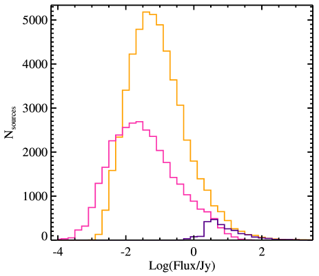
Figure 29: Distributions of fluxes of counterparts of the Hi-GAL sources in the catalogue, at 24 $\mu$m (MIPSGAL, magenta), 22 $\mu$m (WISE, orange), and 21 $\mu$m (MSX, purple).

To quantify this bias between inner and outer Galaxy SEDs, Fig. 29 shows the distributions of MIPSGAL, WISE, and MSX fluxes associated with the Hi-GAL sources in the catalogue. In our sample, MIPSGAL seems to be around 3 times (0.5 in logarithm) more sensitive than WISE. From the standpoint of completeness, in the inner Galaxy sources with $F_{24}>0.03$ Jy have a good chance of being detected in MIPSGAL, whereas in the outer Galaxy sources need to have $F_{22}>0.1$ Jy. Thus in the outer Galaxy many more potential source counterparts will remain undetected in the MIR. Finally, it can be seen that MSX fluxes are all above 1 Jy.

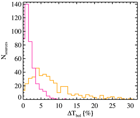
Figure 30: Distributions of the percentage increase of $T_{\textrm{bol}}$ for relatively faint ($F_{70}<2$ Jy) and MIR-dark Hi-GAL sources produced by extending their SED with a MIR flux at the corresponding survey completeness limit (cf. Fig. 29): MIPSGAL, $F_{24}=0.03$ Jy at 24 $\mu$m (magenta) and WISE, $F_{22}=0.1$ Jy at 22 $\mu$m (orange).

Consequently, it is important to quantify how the bolometric temperature (Section 4.4) is underestimated by the failure to detect a faint MIR counterpart. A simple way to evaluate this for a Hi-GAL SED without a MIR flux is to artificially add a flux close to the apparent completeness limit of WISE or MIPSGAL at 22 or 24 $\mu$m, respectively. To consider only realistic cases, we chose relatively faint MIR-dark protostellar sources by imposing $F_{70}<2$ Jy (419 sources). We recalculated the bolometric temperature after adding a hypothetical detection of $F_{22}=0.1$ Jy at 22 $\mu$m, or $F_{24}=0.03$ Jy at 24 $\mu$m, respectively, to their SED. The percentage increases in $T_{\textrm{bol}}$ are given in Fig. 30.

The case of WISE is relevant to the entire sky area covered by Hi-GAL and as expected shows a larger effect than for MIPSGAL. Although the increase can reach 30 per cent, the 90th percentile is 16.3 per cent, and the median 6.7 per cent. The latter is equivalent to the statement that failure to detect the MIR source in WISE near the sensitivity limit leads typically to an underestimate of $T_{\textrm{bol}}$ by about 7 per cent. For sources with Herschel fluxes larger than those used in this test, this effect would be even lower because an even greater portion of the integral of the SED is produced at lower frequencies.

Sources at longitudes $-68^{\circ}<\ell<69^{\circ}$ (cf. Fig. 1) can benefit from the better sensitivity achieved by MIPSGAL at 24 $\mu$m. In this case, our test predicts a median underestimate of $T_{\textrm{bol}}$ by just 1.8 per cent. Starting from the definition of $T_{\textrm{bol}}$ (Myers & Ladd, 1993), it is possible to show that the variations produced by introducing a flux at relatively similar frequencies (as is the case for WISE and MIPSGAL) are in a nearly constant ratio, dependent on the fluxes set for the test. The ratio is about 3.67 in this specific case, in agreement with the median values found for the two cases.

Author afilliations
¹INAF-IAPS, via del Fosso del Cavaliere 100, I-00133 Roma, Italy
²Departamento de Astronomía, Universidad de Chile, Casilla 36-D, Santiago, Chile
³Aix Marseille Univ., CNRS, LAM, Laboratoire d’Astrophysique de Marseille, Marseille, France
⁴Institut Universitaire de France, Paris, France
⁵Canadian Institute for Theoretical Astrophysics, University of Toronto, McLennan Physical Laboratories, 60 St. George Street, Toronto, Ontario, Canada
⁶INAF, Osservatorio Astrofisico di Arcetri, Largo E. Fermi 5, I-50125, Firenze, Italy
⁷Department of Physics & Astronomy, University of Calgary, AB, T2N 1N4, Canada
⁸School of Physics and Astronomy, Cardiff University, Cardiff CF24 3AA, Wales, UK
⁹Astrophysics Research Institute, Liverpool John Moores University, Liverpool Science Park Ic2, 146 Brownlow Hill, Liverpool, L3 5RF, UK
¹⁰Space Telescope Science Institute, 3700 San Martin Dr., Baltimore, MD, 21218, USA
¹¹Infrared Processing Analysis Center, California Institute of Technology, Pasadena, CA 91125, USA
¹²Instituto de Astrofísica e Ciências do Espaço, Universidade do Porto, CAUP, Rua das Estrelas, PT4150-762 Porto, Portugal
¹³European Space Agency (ESA), European Space Research and Technology Centre (ESTEC), Keplerlaan 1, 2201 AZ Noordwijk, The Netherlands
¹⁴Italian ALMA Regional Centre, INAF-IRA, Via P. Gobetti 101, I-40129, Bologna, Italy
¹⁵I. Physikalisches Institut, Universität zu Köln, Zülpicher Str. 77, D-50937 Köln, Germany
¹⁶Dipartimento di Matematica e Fisica, Università del Salento, I-73100, Lecce, Italy
¹⁷INAF - Sezione di Lecce, via Arnesano km 5, 73100, Lecce, Italy
¹⁸Dept. of Space, Earth & Environment, Chalmers University of Technology, Gothenburg, Sweden
¹⁹Dept. of Astronomy, University of Virginia, Charlottesville, Virginia 22904, USA
²⁰Center for Interdisciplinary Exploration and Research in Astrophysics and Department of Physics and Astronomy, Northwestern University,
2145 Sheridan Road, Evanston, IL 60208-3112, USA
²¹Center for Astrophysics and Space Astronomy, University of Colorado, Boulder, CO, 80309, USA
²²Konkoly Observatory, Research Centre for Astronomy and Earth Sciences, Konkoly-Thege Miklós út 15-17, 1121 Budapest, Hungary
²³INAF - Osservatorio Astronomico di Roma, via di Frascati 33, I-00078, Monte Porzio Catone, Italy
²⁴Dipartimento di Fisica, Università di Roma “Tor Vergata”, Via della Ricerca Scientifica 1, I-00133, Roma, Italy
²⁵DIET, Università di Roma “La Sapienza”, I-00185 Roma, Italy

References

- Anderson & Bania (2009) Anderson L. D., Bania T. M., 2009, ApJ, 690, 706
- Anderson et al. (2012) Anderson L. D., et al., 2012, A&A, 542, A10
- Anderson et al. (2014) Anderson L. D., Bania T. M., Balser D. S., Cunningham V., Wenger T. V., Johnstone B. M., Armentrout W. P., 2014, ApJS, 212, 1
- André et al. (2000) André P., Ward-Thompson D., Barsony M., 2000, Protostars and Planets IV, p. 59
- Baldeschi et al. (2017a) Baldeschi A., et al., 2017a, MNRAS, 466, 3682
- Baldeschi et al. (2017b) Baldeschi A., Molinari S., Elia D., Pezzuto S., Schisano E., 2017b, MNRAS, 472, 1778
- Battersby et al. (2014) Battersby C., Ginsburg A., Bally J., Longmore S., Dunham M., Darling J., 2014, ApJ, 787, 113
- Battersby et al. (2017) Battersby C., Bally J., Svoboda B., 2017, ApJ, 835, 263
- Beckwith & Sargent (1991) Beckwith S. V. W., Sargent A. I., 1991, ApJ, 381, 250
- Bergin & Tafalla (2007) Bergin E. A., Tafalla M., 2007, ARA&A, 45, 339
- Bernard et al. (2010) Bernard J.-P., et al., 2010, A&A, 518, L88
- Blitz et al. (1982) Blitz L., Fich M., Stark A. A., 1982, ApJS, 49, 183
- Brand et al. (2001) Brand J., Wouterloot J. G. A., Rudolph A. L., de Geus E. J., 2001, A&A, 377, 644
- Bressert et al. (2012) Bressert E., Ginsburg A., Bally J., Battersby C., Longmore S., Testi L., 2012, ApJ, 758, L28
- Bronfman et al. (1988) Bronfman L., Cohen R. S., Alvarez H., May J., Thaddeus P., 1988, ApJ, 324, 248
- Butler & Tan (2012) Butler M. J., Tan J. C., 2012, ApJ, 754, 5
- Cesaroni et al. (2015) Cesaroni R., et al., 2015, A&A, 579, A71
- Chen et al. (1995) Chen H., Myers P. C., Ladd E. F., Wood D. O. S., 1995, ApJ, 445, 377
- Compiègne et al. (2010) Compiègne M., Flagey N., Noriega-Crespo A., Martin P. G., Bernard J. P., Paladini R., Molinari S., 2010, ApJ, 724, L44
- Csengeri et al. (2014) Csengeri T., et al., 2014, A&A, 565, A75
- Désert et al. (2008) Désert F. X., et al., 2008, A&A, 481, 411
- Djordjevic et al. (2019) Djordjevic J. O., Thompson M. A., Urquhart J. S., Forbrich J., 2019, MNRAS, 487, 1057
- Dobbs & Burkert (2012) Dobbs C. L., Burkert A., 2012, MNRAS, 421, 2940
- Dowell et al. (2003) Dowell C. D., et al., 2003, in Phillips T. G., Zmuidzinas J., eds, Society of Photo-Optical Instrumentation Engineers (SPIE) Conference Series Vol. 4855, Millimeter and Submillimeter Detectors for Astronomy. pp 73–87, doi:10.1117/12.459360
- Duarte-Cabral et al. (2013) Duarte-Cabral A., Bontemps S., Motte F., Hennemann M., Schneider N., André P., 2013, A&A, 558, A125
- Dunham et al. (2013) Dunham M. M., et al., 2013, AJ, 145, 94
- Eden et al. (2015) Eden D. J., Moore T. J. T., Urquhart J. S., Elia D., Plume R., Rigby A. J., Thompson M. A., 2015, MNRAS, 452, 289
- Egan et al. (2003) Egan M. P., et al., 2003, VizieR Online Data Catalog, 5114, 0
- Elia (2020) Elia D., 2020, Communications of the Byurakan Astrophysical Observatory, 67, 241
- Elia & Pezzuto (2016) Elia D., Pezzuto S., 2016, MNRAS, 461, 1328
- Elia et al. (2013) Elia D., et al., 2013, ApJ, 772, 45
- Elia et al. (2017) Elia D., et al., 2017, MNRAS, 471, 100
- Evans et al. (2001) Evans Neal J. I., Rawlings J. M. C., Shirley Y. L., Mundy L. G., 2001, ApJ, 557, 193
- Fehér et al. (2017) Fehér O., Juvela M., Lunttila T., Montillaud J., Ristorcelli I., Zahorecz S., Tóth L. V., 2017, A&A, 606, A102
- Giannetti et al. (2017) Giannetti A., et al., 2017, A&A, 606, L12
- Giannini et al. (2012) Giannini T., et al., 2012, A&A, 539, A156
- Ginsburg et al. (2013) Ginsburg A., et al., 2013, ApJS, 208, 14
- Griffin et al. (2010) Griffin M. J., et al., 2010, A&A, 518, L3
- Gutermuth & Heyer (2015) Gutermuth R. A., Heyer M., 2015, AJ, 149, 64
- Guzmán et al. (2015) Guzmán A. E., Sanhueza P., Contreras Y., Smith H. A., Jackson J. M., Hoq S., Rathborne J. M., 2015, ApJ, 815, 130
- Heyer & Dame (2015) Heyer M., Dame T. M., 2015, ARA&A, 53, 583
- Heyer et al. (1998) Heyer M. H., Brunt C., Snell R. L., Howe J. E., Schloerb F. P., Carpenter J. M., 1998, ApJS, 115, 241
- Hoare et al. (2012) Hoare M. G., et al., 2012, PASP, 124, 939
- Honma et al. (2011) Honma M., Hirota T., Kan-Ya Y., Kawaguchi N., Kobayashi H., Kurayama T., Sato K., 2011, PASJ, 63, 17
- Hou et al. (2009) Hou L. G., Han J. L., Shi W. B., 2009, A&A, 499, 473
- Jackson et al. (2013) Jackson J. M., et al., 2013, Publ. Astron. Soc. Australia, 30, e057
- Kainulainen et al. (2011) Kainulainen J., Beuther H., Banerjee R., Federrath C., Henning T., 2011, A&A, 530, A64
- Kauffmann & Pillai (2010) Kauffmann J., Pillai T., 2010, ApJ, 723, L7
- König et al. (2017) König C., et al., 2017, A&A, 599, A139
- Krumholz & McKee (2008) Krumholz M. R., McKee C. F., 2008, Nature, 451, 1082
- Larson (1981) Larson R. B., 1981, MNRAS, 194, 809
- Li et al. (2017) Li J. I.-H., Liu H. B., Hasegawa Y., Hirano N., 2017, ApJ, 840, 72
- Lippok et al. (2016) Lippok N., et al., 2016, A&A, 592, A61
- Liu et al. (2018) Liu X.-L., Xu J.-L., Ning C.-C., Zhang C.-P., Liu X.-T., 2018, Research in Astronomy and Astrophysics, 18, 004
- López-Sepulcre et al. (2010) López-Sepulcre A., Cesaroni R., Walmsley C. M., 2010, A&A, 517, A66
- Luna et al. (2006) Luna A., Bronfman L., Carrasco L., May J., 2006, ApJ, 641, 938
- Ma et al. (2013) Ma B., Tan J. C., Barnes P. J., 2013, ApJ, 779, 79
- Martin et al. (2012) Martin P. G., et al., 2012, ApJ, 751, 28
- Mathis et al. (1983) Mathis J. S., Mezger P. G., Panagia N., 1983, A&A, 500, 259
- Maury et al. (2011) Maury A. J., André P., Men’shchikov A., Könyves V., Bontemps S., 2011, A&A, 535, A77
- Mège et al. (2021) Mège P., et al., 2021, A&A, 646, A74
- Merello et al. (2015) Merello M., Evans II N. J., Shirley Y. L., Rosolowsky E., Ginsburg A., Bally J., Battersby C., Dunham M. M., 2015, ApJS, 218, 1
- Merello et al. (2019) Merello M., et al., 2019, MNRAS, 483, 5355
- Mezger (1990) Mezger P. G., 1990, in Bowyer S., Leinert C., eds, IAU Symposium Vol. 139, The Galactic and Extragalactic Background Radiation. p. 63
- Miville-Deschênes et al. (2017) Miville-Deschênes M.-A., Murray N., Lee E. J., 2017, ApJ, 834, 57
- Moffat et al. (1979) Moffat A. F. J., Fitzgerald M. P., Jackson P. D., 1979, A&AS, 38, 197
- Molinari et al. (2008) Molinari S., Pezzuto S., Cesaroni R., Brand J., Faustini F., Testi L., 2008, A&A, 481, 345
- Molinari et al. (2010) Molinari S., et al., 2010, PASP, 122, 314
- Molinari et al. (2011) Molinari S., Schisano E., Faustini F., Pestalozzi M., di Giorgio A. M., Liu S., 2011, A&A, 530, A133
- Molinari et al. (2016a) Molinari S., et al., 2016a, A&A, 591, A149
- Molinari et al. (2016b) Molinari S., Merello M., Elia D., Cesaroni R., Testi L., Robitaille T., 2016b, ApJ, 826, L8
- Molinaro et al. (2016) Molinaro M., et al., 2016, in Chiozzi G., Guzman J. C., eds, Society of Photo-Optical Instrumentation Engineers (SPIE) Conference Series Vol. 9913, Software and Cyberinfrastructure for Astronomy IV. p. 99130H (arXiv:1608.04526), doi:10.1117/12.2231674
- Momany et al. (2006) Momany Y., Zaggia S., Gilmore G., Piotto G., Carraro G., Bedin L. R., de Angeli F., 2006, A&A, 451, 515
- Motte et al. (2010) Motte F., et al., 2010, A&A, 518, L77
- Mottram et al. (2011) Mottram J. C., et al., 2011, ApJ, 730, L33
- Mueller et al. (2002) Mueller K. E., Shirley Y. L., Evans II N. J., Jacobson H. R., 2002, ApJS, 143, 469
- Myers & Ladd (1993) Myers P. C., Ladd E. F., 1993, ApJ, 413, L47
- Nakanishi & Sofue (2006) Nakanishi H., Sofue Y., 2006, PASJ, 58, 847
- Ossenkopf & Henning (1994) Ossenkopf V., Henning T., 1994, A&A, 291, 943
- Paladini et al. (2012) Paladini R., et al., 2012, ApJ, 760, 149
- Paradis et al. (2014) Paradis D., et al., 2014, A&A, 572, A37
- Pattle (2016) Pattle K., 2016, MNRAS, 459, 2651
- Peretto et al. (2013) Peretto N., et al., 2013, A&A, 555, A112
- Pilbratt et al. (2010) Pilbratt G. L., et al., 2010, A&A, 518, L1
- Poglitsch et al. (2010) Poglitsch A., et al., 2010, A&A, 518, L2
- Portegies Zwart et al. (2010) Portegies Zwart S. F., McMillan S. L. W., Gieles M., 2010, ARA&A, 48, 431
- Purcell et al. (2013) Purcell C. R., et al., 2013, ApJS, 205, 1
- Ragan et al. (2016) Ragan S. E., Moore T. J. T., Eden D. J., Hoare M. G., Elia D., Molinari S., 2016, MNRAS, 462, 3123
- Rigby et al. (2016) Rigby A. J., et al., 2016, MNRAS, 456, 2885
- Rigby et al. (2019) Rigby A. J., et al., 2019, A&A, 632, A58
- Roman-Duval et al. (2010) Roman-Duval J., Jackson J. M., Heyer M., Rathborne J., Simon R., 2010, ApJ, 723, 492
- Rosolowsky et al. (2010) Rosolowsky E., et al., 2010, ApJS, 188, 123
- Russeil et al. (2011) Russeil D., et al., 2011, A&A, 526, A151
- Russeil et al. (2017) Russeil D., Zavagno A., Mège P., Poulin Y., Molinari S., Cambresy L., 2017, A&A, 601, L5
- Sadavoy et al. (2016) Sadavoy S. I., Stutz A. M., Schnee S., Mason B. S., Di Francesco J., Friesen R. K., 2016, A&A, 588, A30
- Schlingman et al. (2011) Schlingman W. M., et al., 2011, ApJS, 195, 14
- Schuller et al. (2009) Schuller F., et al., 2009, A&A, 504, 415
- Smith (2014) Smith M. D., 2014, MNRAS, 438, 1051
- Sofue & Nakanishi (2016) Sofue Y., Nakanishi H., 2016, PASJ, 68, 63
- Svoboda et al. (2016) Svoboda B. E., et al., 2016, ApJ, 822, 59
- Tan et al. (2013) Tan J. C., Kong S., Butler M. J., Caselli P., Fontani F., 2013, ApJ, 779, 96
- Traficante et al. (2017) Traficante A., Fuller G. A., Billot N., Duarte-Cabral A., Merello M., Molinari S., Peretto N., Schisano E., 2017, MNRAS, 470, 3882
- Traficante et al. (2018) Traficante A., et al., 2018, MNRAS, 477, 2220
- Urquhart et al. (2013a) Urquhart J. S., et al., 2013a, MNRAS, 431, 1752
- Urquhart et al. (2013b) Urquhart J. S., et al., 2013b, MNRAS, 435, 400
- Urquhart et al. (2014) Urquhart J. S., et al., 2014, MNRAS, 443, 1555
- Urquhart et al. (2018) Urquhart J. S., et al., 2018, MNRAS, 473, 1059
- Wienen et al. (2015) Wienen M., et al., 2015, A&A, 579, A91
- Wright et al. (2010) Wright E. L., et al., 2010, AJ, 140, 1868
- Xu et al. (2016) Xu Y., et al., 2016, Science Advances, 2, e1600878
- Yuan et al. (2017) Yuan J., et al., 2017, ApJS, 231, 11
- Zahorecz et al. (2016) Zahorecz S., Jimenez-Serra I., Wang K., Testi L., Tóth L. V., Molinari S., 2016, A&A, 591, A105
- Zetterlund et al. (2018) Zetterlund E., Glenn J., Rosolowsky E., 2018, MNRAS, 480, 893
- Zhang et al. (2020) Zhang S., et al., 2020, A&A, 637, A40