Exploring the Early Universe with Gaia and THEIA

Abstract

It has recently been pointed out that Gaia is capable of detecting a stochastic gravitational wave background in the sensitivity band between the frequency of pulsar timing arrays and LISA. We argue that Gaia and THEIA has great potential for early universe cosmology, since such a frequency range is ideal for probing phase transitions in asymmetric dark matter, SIMP and the cosmological QCD transition. Furthermore, there is the potential for detecting primordial black holes in the solar mass range produced during such an early universe transition and distinguish them from those expected from the QCD epoch. Finally, we discuss the potential for Gaia and THEIA to probe topological defects and the ability of Gaia to potentially shed light on the recent NANOGrav results.

1 Introduction

It has recently been shown that large surveys of stars such as Gaia Brown:2018dum and the proposed upgrade, THEIA (Telescope for Habitable Exoplanets and Interstellar/Intergalactic Astronomy) 10.3389/fspas.2018.00011 , can be powerful probes of gravitational waves (GW) Moore:2017ity . GWs affect the apparent position of a star, and the multiple subsequent measurements of the same star can be used to turn Gaia into a GW observatory Moore:2017ity ; Mihaylov:2018uqm ; Mihaylov:2019lft . The dimensionless strain sensitivity of Gaia is expected to be a constant Moore:2017ity and scale inversely with the lifetime of the experiment Book:2010pf . This is in contrast to pulsar timing arrays, whose strain sensitivity scales as the inverse square root of the observation time. The scaling with the mission lifetime comes from the fact that Gaia monitors the position of $N$ sources in the sky with angular resolution $\Delta\theta$ over a time $T$. For a single source, one could detect an angular velocity (proper motion) of order $\Delta\theta/T$, and for $N$ sources, a correlated angular velocity of order $\Delta\theta/(T\sqrt{N})$ should be detectable. It follows Book:2010pf that one should obtain an upper limit

$$\Omega_{\rm gw}(f\sim 1/T)\lower 3.01385pt\hbox{$\;\stackrel{{\scriptstyle\textstyle<}}{{\sim}}\;$}\frac{\Delta\theta^{2}}{NT^{2}H_{0}^{2}}$$ (1)

on the GW energy density from a SGWB. Moreover, the analysis of Ref. Moore:2017ity seems to indicate that the cadence of the astrometric survey does not change the strain sensitivity appreciably, at least not more than an order of magnitude.

The constant strain sensitivity makes astrometry a powerful tool for filling the sensitivity gap between nanohertz frequencies probed at pulsar timing arrays Lentati:2015qwp ; Arzoumanian:2020vkk , and millihertz frequencies probed by the LISA mission Bartolo:2016ami . Furthermore, the efficient scaling with the mission time makes upgrades to Gaia competitive with even the square kilometer array at probing the nanohertz range. In this paper we discuss the cosmological opportunities of using Gaia and THEIA as GW observatories. In particular, various dark matter models based on the Strongly-Interacting Massive Particles (SIMP) paradigm are expected to feature a confining transition that could leave a observable background gravitational wave spectrum that typically peaks between the sensitivity ranges of LISA and pulsar timing arrays, precisely the frequency range where astrometry can contribute. Asymmetric dark matter is also expected to include physics at a similar scale. Further we explore the potential of primordial black hole detection with an emphasis of primordial black hole production during such a confining transition. We also discuss the potential to observe gravitational wave backgrounds generated from topological defects such as domain walls and strings. Finally, motivated by the recent hint of a possible SGWB signal at NANOGrav Arzoumanian:2020vkk , we discuss the timescale for Gaia to give complementary information on the tentative signal.

The structure of this paper is as follows. Section 2 we give the sensitivity curves for Gaia and its upgrades, we then discuss the potential to observe cosmological phase transitions indirectly with astrometry in Section 3. Note that in that section we discuss specific models that can be detected, focusing on dark sectors. Next, in section 4, we discuss cosmological defects and the potential reach of astrometry as well as a discussion of the recent NANOGrav results. In section 5 we discuss the effect that phase transitions have on the Primordial Black Hole (PBH) mass spectrum as a complementary cosmological probe before concluding in section 6. We describe in the Appendices the low-energy effective models associated with confinement transitions.

2 Sensitivity curves for Gaia and THEIA

Experimental designs typically specify a strain sensitivity, whereas cosmologists are typically interested in the gravitational wave abundance. The strain sensitivity, $h_{\rm gw}$ can be conveniently converted to the abundance, $\Omega_{\rm GW}$ via the relation

$$\Omega_{\rm gw}(f)\,h^{2}=\frac{2\pi^{2}}{3H_{0}^{2}}f^{2}h_{\rm gw}^{2}(f)h^{2}$$ (2)

where $h=0.67$, i.e. $H_{0}=67$ (km/s)/Mpc, is the value of Hubble observed today and $f$ is the frequency. For Gaia we can take the constant sensitivity derived in ref. Moore:2017ity

$$h_{\rm GW}=10^{-14}\left(\frac{5\ {\rm years}}{T_{M}}\right),\ \forall\ f>1/T_{M}$$ (3)

where $T_{M}$ is the mission lifetime, which we will generously take to be $~{}20$ years. For THEIA, we estimate that one will observe a hundred times as many stars with an angular velocity resolution that is superior by a factor of 60. This results in a strain sensitivity of

$$h_{\rm GW}=1.6\times 10^{-16}\left(\frac{5\ {\rm years}}{T_{M}}\right),\ \forall\ f>1/T_{M}\ .$$ (4)

When searching for a specific signal, the sensitivity of Gaia can be dramatically improved by comparing the signal for multiple frequencies. We present the peak integrated sensitivity curve Schmitz:2020syl relevant for phase transitions and the power law sensitivity curve Thrane:2013oya relevant for strings in Fig. 1. In both cases the integrated sensitiviity curve can be obtained by

$${\cal N}(f) = \left(3H_{0}^{2}\int_{f_{\rm min}=1/T}^{f_{\rm max}}\left(\frac{f^{\prime}}{f}\right)^{3}\left(\frac{7}{4+3\left(4+3\left(\frac{f^{\prime}}{f}\right)^{2}\right)}\right)^{7/2}\frac{df^{\prime}}{2\pi^{2}(f^{\prime})^{3}h_{\rm GW}^{2}h^{2}}\right)^{-1}$$ (5)

$${\cal N}(f) = {\rm Max}(n)\left[\left(\frac{f}{f_{\rm min}}\right)^{n}\left(3H_{0}^{2}\int_{f_{\rm min}=1/T}^{f_{\rm max}}\frac{(f^{\prime}/f_{\rm min})^{n}}{2\pi^{2}(f^{\prime})^{3}h_{\rm GW}^{2}h^{2}}df^{\prime}\right)^{-1}\right]\,,$$ (6)

for a broken and an envelope of power laws respectively. The sensitivity we show in Fig. 1 alongside pulsar timing arrays as well as other proposed experiments including Lisa and aLIGO. THEIA is almost unmatched in its potential sensitivity and both astrometry experiments have reach in between that seen by pulsar timing arrays and LISA.

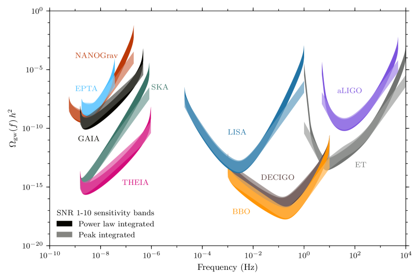
Figure 1: Power law and peak integrated sensitivity curves for pulsar timing arrays vanHaasteren:2011ni ; Janssen:2014dka ; Lazio:2018ukb against astrometry methods such as Gaia and THEIA. The bands correspond to a signal to noise ratio between 1 and 10, the lighter bands are power law integrated sensitivity curves while the darker bands correspond to the peak integrated sensitivity bands. Also included are space based missions, Lisa Caprini:2019egz , BBO Yagi:2011wg and Decigo Kawamura:2006up ; Kawamura:2020pcg where for the latter we have used the ultimate specifications. Additionally, we included high frequency detectors in aLIGO TheLIGOScientific:2014jea and the Einstein telecope Punturo:2010zz . Note that THEIA has sensitivity in the range beween pulsar timing arrays and LISA. By extending the cadence of THEIA down to days one could fill the gap between PTA and LISA frequencies.

3 Phase transitions

For any given phase transition, the dominant source is widely believed to be the acoustic source Hindmarsh:2013xza ; Hindmarsh:2015qta ; Hindmarsh:2017gnf . The spectral form is model independent with the peak amplitude and frequency depending just on four thermal parameters - the bubble wall velocity, $v_{w}$, the inverse timescale of the transition, $\beta$, the change in the trace anomaly normalized by the radiation density, $\alpha$, and the temperature at which percolation occurs, $T_{p}$. The peak amplitude depends on the thermal parameters as follows Hindmarsh:2013xza ; Hindmarsh:2015qta ; Hindmarsh:2017gnf ; Guo:2020grp

$$h^{2}\Omega_{\text{GW}}=8.5\times 10^{-6}\left(\frac{100}{g_{s}(T_{e})}\right)^{1/3}\Gamma^{2}\bar{U}_{f}^{4}\left[\frac{H_{s}}{\beta(v_{w})}\right]v_{w}\times\Upsilon,$$ (7)

where $\Gamma\sim 4/3$ is the adiabatic index and ${\Upsilon}$ is the suppression factor arising from the finite lifetime, $\tau_{\text{sh}}$, of the sound waves, given by

$$\Upsilon=1-\frac{1}{\sqrt{1+2\tau_{\text{sh}H_{s}}}}.$$ (8)

3.1 Motivating first order transitions detectable with astrometry

The range of frequencies that Gaia is sensitive to is ideal for a phase transition occurring between an MeV and a GeV. This is precisely the scale we would expect a confinement transition to occur in either QCD, a hidden sector involving a strongly interacting massive particle (SIMP), or asymmetric dark matter model. In fact, the preferred confinement scale for strongly interacting massive particle (SIMP) dark matter is precisely in this range Hochberg:2014dra . We will focus mostly on hidden sector models here, but let us begin with the QCD transition, which can also in principle be a strong first order transition and can give us insight to what sort of phase transitions can lead to a gravitational wave signature.

In the standard model, the cosmological QCD transition is unfortunately not expected to be strongly first order Bazavov:2011nk ; Gupta:2011wh . However, in principle, extensions to the standard model or unusual conditions in the early Universe could modify this. Confinement transitions are not as easy to model as transitions involving fundamental scalars, where effective potential methods provide a powerful and intuitive guide and are known to describe low scale QCD reasonably well GellMann:1960np ; Nambu:1961tp ; Nambu:1961fr ; Fukushima:2003fw . In the absence of lattice calculations, it is a natural to consider an effective scalar theory and model confinement transitions in an analogous manner. From such an effective theory, one can make a qualitative check of that nature of the transition by searching for stable infrared fixed points Pisarski:1983ms . Between lattice calculations and effective methods of the condensate one can derive three scenarios that can make a cosmological confinement transition first order

• Having at least three quarks that are effectively massless compared to the confinement scale. In QCD, this can occur if $u$, $d$, $s$ quarks are made lighter in the early Universe Davoudiasl:2019ugw .

• Having a pure Yang–Mills transition where quarks are either absent or heavy.

• The baryon chemical potential is large in the early Universe. This can be achieved through a large lepton asymmetry Schwarz:2009ii which can be made compatible with BBN bounds Barenboim:2016shh . In principle a confinement transition in a SIMP model can be similarly influenced by a large asymmetry in the early Universe.

Although the calculations we present here will suffer from theoretical uncertainty, results do seem to agree with the intuition that the larger the change in relativistic degrees of freedom, the stronger the transition. For example, in the case where glueballs dominate the confining transition, the strength of the transition grows with the number of colors. Similarly, in the case where quark condensates dominate the free energy, prior work has shown some evidence that strength of the transition grows with the number of flavours Croon:2019iuh . We will also consider the implications of a transition of a fundamental scalar in an asymmetric dark matter model introduced in ref. Croon:2019rqu .

3.1.1 Gravitational waves from chiral symmetry breaking

To estimate the gravitational wave signal in a chiral symmetry breaking transition, we follow the strategy of recent work that relies on low energy effective theories such as the linear sigma model (LSM) and the (p)NJL model Helmboldt:2019pan . The NJL has the advantage of being sensitive to the number of colours in the theory whereas the LSM is sensitive only to the number of quark flavours. The pNJL model improves on the NJL model yet again by including a potential for Wilson loops whose coefficients can be derived from lattice Roessner:2006xn . There is to date no lattice calculation to compare the predictions for the gravitational wave signal produced in either model, we therefore simply calculate benchmarks in each model with the expectation that there can be future improvement in the predictions of gravitational waves produced in SIMP models.

For the linear sigma model, a large gravitational wave signal is predicted in the case where there is a large hierarchy between the axion and pion mass Croon:2019iuh . In the case of the (p)NJL model, there is a critical point in the parameter space where it no longer is energetically favourable for chiral symmetry breaking to occur. Near this critical point are the strongest transitions and we choose benchmarks in this region of parameter space. To ascertain the lowest temperature a confinement transition can occur we need to enforce a number of conditions

• To drain the entropy in the hidden sector we require kinetic equilibrium to be maintained until the freeze out temperature - typically one twentieth the pion mass Hochberg:2014dra ; Hochberg:2015vrg .

• We enforce the chiral limit, this means the pion mass is much lower than the critical temperature. We do not have a precise criteria, but for our present purposes require that the critical temperature to be ten times the pion mass.

• Freezeout needs to occur well before BBN. To ensure safety we enforce a conservative bound that $T_{\rm FO}>2$ MeV.

Let us begin with the first criteria. We must ensure that kinetic equilibrium is maintained at the freeze-out temperature to ensure the entropy is drained . We consider dark photon mediation between mesons and SM fermions as the channel to maintain equilibrium Hochberg:2015vrg ; Kuflik:2015isi . This is achieved when,

$$\frac{5\zeta(5)}{4}m_{\pi}\Gamma_{\rm scatt}\lesssim\frac{H(T_{f})m_{\pi}^{2}}{T_{f}}$$ (9)

where

$$\Gamma_{\rm scatt}=\sum_{f}\frac{\sigma_{f}v_{\rm rel}}{E_{f}^{2}}\frac{12\zeta(5)}{\pi^{2}}\frac{15}{16}T_{f}^{5}$$ (10)

and

$$\sigma_{f}v_{\rm rel} = 8\pi\alpha_{D}\alpha\sum\frac{Q_{\pi}^{2}}{N_{\pi}}\frac{1}{c_{\chi}^{2}}\left[-\left(\frac{c_{\zeta}^{2}}{m_{V}^{2}}+\frac{s_{\zeta}^{2}}{m_{Z}^{2}}\right)c_{W}t_{\chi}Q_{f}\right.$$ (11)

$$\left.+\left(\frac{c_{\zeta}(s_{\zeta}+s_{W}t_{\chi}c_{\zeta})}{m_{V}^{2}}-\frac{s_{\zeta}(c_{\zeta}-s_{W}t_{\chi}s_{\xi})}{m_{Z}^{2}}\right)\frac{1}{s_{W}c_{W}}(I_{3}^{f}-Q_{f}s_{W}^{2})\right]E_{f}^{2}\ .$$

In the above we follow the notational conventions of ref. Hochberg:2015vrg . Specifically, $(s_{x},t_{x},c_{x})$ denote trigonometric functions where the subscript denotes the argument. The angle, $\chi$ is the mixing

$$L\supset-\frac{\sin\chi}{2}B^{\mu\nu}A^{\mu\nu}\ ,$$ (12)

and

$$\tan 2\zeta=\frac{m_{Z}^{2}s_{W}\sin 2\chi}{m_{V}^{2}-m_{Z}^{2}(c_{\chi}^{2}-s_{W}^{2}s_{\chi}^{2})}\ .$$ (13)

Furthermore, $\pi$ denotes the dark pion, $\alpha_{D}$ denotes the dark sector coupling strength and all Standard Model notation is conventional. It is straightforward to achieve kinetic equilibrium and avoid all possible dark photon constraints Fradette:2014sza for a remarkably low freezeout temperatures when the mixing is of the order $\chi\sim 10^{-4}$.

The second and third constraints are arguably the most restricting. If the freezeout temperature is at least 2 MeV, this implies a pion mass of at least 40 MeV which in turn implies a critical temperature of 400 MeV. This of course does not necessarily exclude interesting gravitational wave signatures from a SIMP with light quarks involving a much lower critical temperature. The weakness of the limit arising from kinetic equilibrium at freeze-out is very promising. However, the methods for calculating such a gravitational wave signal is even more uncertain than what we present as the chiral limit becomes invalid. With these restrictions in mind, we therefore present the conservative benchmarks presented in Table 1 with the GW signal plotted in Figs. 2 and 3. Note that even THEIA requires a reasonably strong phase transition, so in general the percolation temperature can be well below the transition temperature. We take the chiral limit as being valid when the critical temperature is $400$ MeV and the transition occurs when kinetic equilibrium is still possible. This can mean in some benchmarks that the mass of the quarks are not too light compared to the transition temperature. There is a theoretical uncertainty that arises from this that needs to be settled either by lattice modelling or substantial theoretical progress.

Model	$N_{C}$	$N_{F}$	$\Lambda$	parameters
LSM	N/A	4	-	$m_{A}/m_{\phi}=51.66$
NJL ($B_{2}$)	3	3	$1.24$ GeV	$G^{-1}=0.48$ GeV2, $G_{D}^{-1}=-0.042$ GeV5
NJL ($B_{3}$)	5	3	$4$ GeV	$G^{-1}=9.79$ GeV2, $G_{D}^{-1}=-14.72$ GeV5
pNJL ($B_{4}$)	3	3	$6.2$ GeV	$G^{-1}=11.97$ GeV2, $G_{D}^{-1}=-131.69$ GeV5

Table 1: Benchmarks for SIMP models with light quarks. In each case the critical temperature is set to the conservative limit of 400 MeV (see text for explanation). The number of flavours is denoted by $N_{F}$ and the number of colours by $N_{C}$. The parameters are found by tuning the critical temperature to 400 MeV and notational conventions are taken from ref. Hochberg:2015vrg .

3.2 Asymmetric dark matter and solitosynthesis

If a phase transition has tunneling rate that never becomes large enough compared to the Hubble time to percolate, the phase transition can still complete through a process known as solitosynthesis so long as there is a conserved charge to stabilize sub-critical bubbles Kusenko:1997hj . If there is a conserved charge, the free energy of a sub-critical bubble is stabilized by a term proportional to the charge density inside the bubble - such a term diverges for vanishing radius. Such a stable field configuration is known as a Q-ball Coleman:1985ki . As the Universe cools, some sub-critical bubbles become critical and explode, completing the phase transition. The phase transition is typically strong and long lasting Croon:2019rqu .

If dark matter is asymmetric, matching the dark matter to its observed value fixes a relationship between the asymmetry and the mass of the dark matter,

$$Y_{\rm DM}m_{\rm DM}\sim 5\times 10^{-10}\ {\rm GeV}\ .$$ (14)

The transition temperature is generally within an order of magnitude of the dark matter. This makes pulsar timing arrays ideal for probing such a phase transition that has an asymmetry $Y_{\rm DM}\sim O(10^{-7})$. Gaia is ideal for probing such asymmetric dark matter scenarios when $Y_{\rm DM}\sim O(10^{-7}-10^{-8})$. Solitosynthesis occurs in a context where the conventional tunneling rate is too slow compared to Hubble. This typically occurs when there is a tree level barrier between a true and false vacuum. The simplest possibility is a dark sector Higgs augmented by a dimension six operator

$$V(h_{D},\phi)=\kappa\phi^{2}h_{D}^{2}+\Lambda^{4}\left[(2-3\alpha)\left(\frac{h_{D}}{v_{D}}\right)^{2}-\left(\frac{h_{D}}{v_{D}}\right)^{4}+\alpha\left(\frac{h_{D}}{v_{D}}\right)^{6}\right]\ .$$ (15)

We present the benchmarks that use the same model as Ref. Croon:2019rqu with two benchmarks presented in Table 2 where the parameter $\alpha$ is varied between $\alpha\in(0.5,2/3)$. The sensitivity of Gaia and THEIA to these benchmarks are given in 2 and Fig. 3.

v	$\Lambda$	$g$	$\eta$
0.06 GeV	0.02 GeV	0.1	$10^{-7}$
0.7 GeV	0.2 GeV	0.1	$10^{-8}$

Table 2: Benchmark parameters used for solitosynthesis following the notational conventions in ref. Croon:2019rqu .

3.2.1 Glueballs

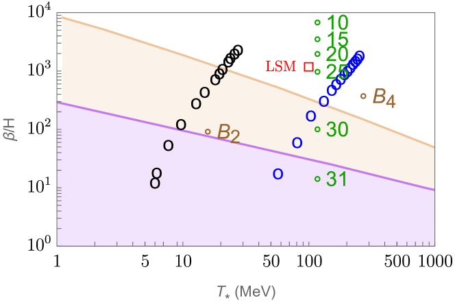
Figure 2: Sensitivity to thermal parameters with $\alpha=1$ and benchmarks for a phase transition from solitosynthesis with asymmetry of $10^{-7}/10^{-8}$ (black/blue circles) glueballs for SU(N) (Olive numbers) and confinement in the LSM model (red squares) and the (p)NJL model. Benchmarks for the (p)NJL model are given in Table 1 are denoted by $B_{x}$. All benchmarks are not excluded from current PTAs. More details on the models producing these transitions are given in the text.

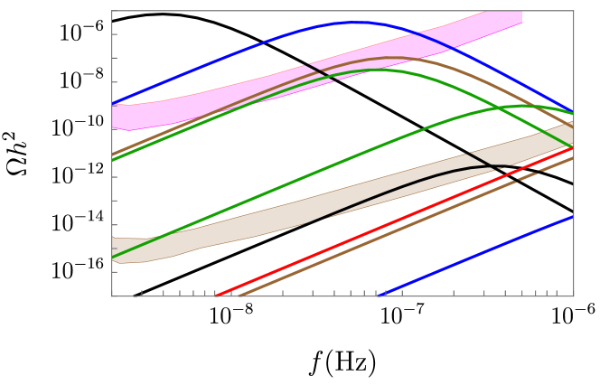
Figure 3: Same models with the same color coding as Fig. 2 against Gaia and THEIA sensitivity curves. In the case of Glueballs we take $N_{C}=30$ and $N_{C}=31$. For solitosynthesis we take the strongest and fifth strongest phase transitions for both values of the dark asymmetry.

Hidden sectors frequently include dark gauge symmetries which can confine. If there are no light fermions in the theory, the properties of the transition can be studied on the lattice without the ambiguities that arise from trying to model fermions. Gravitational waves arising from a pure Yang-Mills confinement transition are particularly attractive as the number of parameters in the theory, specifically the rank of the group and the confinement scale, matches the number of observables in the peak amplitude and frequency of a gravitational wave spectrum. The surface tension and the latent heat of pure Yang Mills confinement transition for a SU($N_{C}$) has been calculated on the lattice for $N_{C}\lesssim 8$ Lucini:2005vg ; Datta:2010sq

$$\sigma=(0.013N_{C}^{3}-0.104)T_{C}^{3}\ ,\quad L=\left(0.549+\frac{0.458}{N_{C}^{2}}\right)T_{C}^{4}\ .$$ (16)

Furthermore, the pressure in each phase is known and the ratio of the pressure to the Stephann-Boltzmann pressure is approximately constant as a function of $N_{C}$ Panero:2009tv . We use lattice results for the pressure of an SU(3) confinement transition from ref. Agasian:2017tag ; Borsanyi:2012ve . In spite of this impressive array of lattice knowledge, the surface tension and latent heat are only calculated at the critical temperature. Similarly, the pressure below the critical temperature is only defined in the confined phase. In the early Universe, the temperature is decreasing fast enough that a fair amount of supercooling can occur by the time percolation begins. To estimate the macroscopic thermal parameters at the percolation temperature requires extrapolation of the lattice results for the supercooled phase. This can be estimated either through a toy potential for the Polyakov loop whose properties match lattice results - either a potential based on the Haar measure Huang:2020mso ; Kang:2021epo or a polynomial potential Halverson:2020xpg ; Kang:2021epo . This presents some challenges, as the growth in the surface tension with $N_{C}$ can be in tension with the fact that the pressure is decreasing much faster than $T^{4}$ near the critical temperature, combined with the fact that the absolute value of the pressure is expected to be negative for strongly super cooled transitions Cohen:2020tgr . Another approach is to use classical nucleation theory and extrapolate the pressure to the super cooled phase.

Since we require a fairly strong transition for it to be visible, we require a fair amount of super-cooling which unfortunately means that any method used will need to be taken with a healthy grain of salt until there are lattice calculations for supercooled transitions. Here we will review classical nucleation theory and apply it to the case of glueball nucleation. The free energy of a bubble of radius $R$ is given by

$$F=-\Delta p\frac{4\pi}{3}R^{3}+\sigma 4\pi R^{2}\ .$$ (17)

Here, $\Delta p$ is the pressure difference between the phases. There is a critical value of $R$ above which it becomes energetically favourable for the bubble to expand as the pressure overwhelms the surface tension. The nucleation rate per unit volume, per unit time is then given by the exponential of the free energy of a critical bubble divided by the temperature

$$\Gamma=T^{4}e^{-16\pi\sigma^{3}/(3T\Delta p^{2})}\ .$$ (18)

To extrapolate the pressure below the critical temperature, we use a linear extrapolation of the pressure, allowing it to go negative. A negative pressure in the supercooled deconfined phase was recently argued for in ref. Cohen:2020tgr . Finally, the inverse time scale of the transition can then be calculated in the usual way $\beta/H=Td[F/T]/dT$.

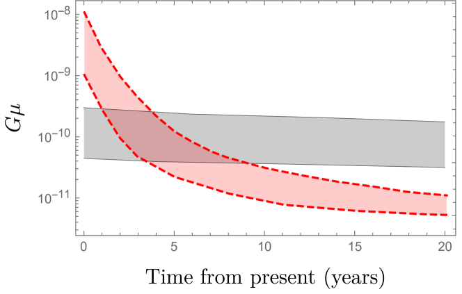
Figure 4: Current and projected reach of NANOGrav (gray) against projected reach of Gaia (red) for cosmic strings with the bands corresponding to a signal to noise ratio SNR $\in(1,10)$.

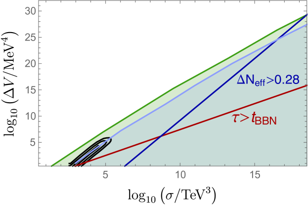
Figure 5: Bottom: Domain walls, Black lines give the 1,2,3 $\sigma$ fits to the potential NANOGrav signal as given in ref Bian:2020bps , olive region is explored by THEIA, light blue region by Gaia. Below the red line the domain wall decays after BBN and below the Brown line the gravitational wave signal is too strong to be compatible with bounds on $\Delta N_{\rm eff}$

While Gaia and THEIA are sensitive to phase transitions occurring at slightly higher frequencies than what would be visible to pulsar timing arrays, it is still optimal for detectability for the transition to occur as late as possible. If the glueballs are absolutely stable on cosmologically relevant lifetimes (i.e. $\tau\gtrsim 10^{25}$s to avoid cmb constraints Chen:2003gz ; Fradette:2014sza ; Yang:2015cva ; Coffey:2020oir ), such glueballs can in principle be dark matter. However, the gravitational wave spectrum is suppressed by eight powers of the temperature ratio between the two sectors as it depends on the square of the latent heat. The temperature ratio is required to be less than one in order to avoid overclosure Forestell:2016qhc ; Forestell:2017wov . Alternatively, one can make the glueballs short lived, in which case their decay rate must be larger than Hubble before BBN in order to avoid changing the expansion rate of the Universe during BBN. If one works through a Higgs portal, the decay rate for a glueball of around the QCD scale is Juknevich:2009ji ; Forestell:2016qhc

$$\Gamma\sim\frac{N^{2}_{C}\Lambda_{x}^{7}y^{2}}{\Lambda^{4}v_{h}^{2}}\ ,$$ (19)

where $N_{C}$ is the number of colors, $\Lambda_{x}$ is the dark confinement scale (we have made the approximation that this is equivalent to the glueball mass) and $y$ is the relevant Yukawa interactions. One can compare this rate to Hubble to find that the minimum scale is the muon threshold, that is $\Lambda\gtrsim 2m_{\mu}$. In the case of vector boson mixing, the rate of Glueball decay is Juknevich:2009gg ; Forestell:2016qhc

$$\Gamma\sim{\alpha_{x}^{2}\alpha_{i}^{2},\alpha_{x}^{3}\alpha_{Y}}N^{2}\frac{\Lambda^{9}_{x}}{\Lambda^{8}}$$ (20)

which allows for a confinement scale of around $100$ MeV for a cutoff scale of around $100$ GeV.

We therefore take this latter value to approximate our confinement transition temperature, though note that it is an approximation and a more detailed calculation could move the lowest possible confinement temperature somewhat.

4 Cosmic Defects and NANOGrav

The recent 12.5 year updated results of NANOGrav observed a stochastic background that is at odds with expected stochastic backgrounds from super massive black hole mergers Arzoumanian:2020vkk . A promising explanation is that the almost scale invariant background generated by cosmic strings Ellis:2020ena ; Blasi:2020mfx ; Datta:2020bht ; Chakrabortty:2020otp ; Samanta:2020cdk ; King:2020hyd . Another possibility is a metastable cosmic string Buchmuller:2020lbh or a domain wall Bian:2020bps ; Craig:2020bnv , a strong first order phase transition Brandenburg:2021tmp ; Li:2021qer ; Lewicki:2020azd ; Neronov:2020qrl ; Nakai:2020oit ; Addazi:2020zcj or primordial black holes Kohri:2020qqd ; Domenech:2020ers ; Sugiyama:2020roc ; DeLuca:2020agl . In the case of metastable strings or domain walls, the low frequency Gravitational wave power spectrum obeys a cubic scaling. In this case, astrometry is an ideal compliment to PTAs as the sensitivity has a better scaling with frequency. We will here focus on stable cosmic strings and domain walls.

Let us begin with the case of a cosmic string. We use the velocity dependent one scale model of ref. Martins:1995tg ; Martins:1996jp ; Martins:2000cs which models the evolution of a loop of length $\ell$ as

$$\ell=\alpha_{\ell}t_{i}-\Gamma G\mu(t-t_{i})$$ (21)

where the emission rate, the string tension and the initial loop size is denoted by $\Gamma\sim 50$ Blanco-Pillado:2013qja ; Blanco-Pillado:2017oxo , $G\mu$ and $\alpha_{\ell}\sim 0.1$ respectively, with our choice for $\alpha_{\ell}$ motivated partly by recent simulations Blanco-Pillado:2013qja ; Blanco-Pillado:2017oxo . The frequency today ($t_{0}$)of the gravitational wave spectrum emitted by a given mode, $k$, can be related to the time of emission, $\tilde{t}$, via

$$f=\frac{a(\tilde{t})}{a(t_{0})}\frac{2k}{\alpha_{\ell}t_{i}-\Gamma G\mu(\tilde{t}-t_{i})}.$$ (22)

The gravitational wave abundance is the sum of the gravitational wave spectrum for individual modes

$$\Omega_{\rm GW}(f)=\sum_{k=1}^{\infty}k\Gamma^{(k)}\Omega_{\rm GW}^{(k)}(f)\ ,$$ (23)

where

$$\Gamma^{(k)}=\frac{\Gamma k^{-4/3}}{\sum_{m=1}^{\infty}m^{-4/3}}\sim 13.9k^{-4/3}\ .$$ (24)

The contribution to the spectrum from each mode has the form

$$\Omega^{(k)}_{\rm GW}(f)=\frac{16\pi}{3H_{0}^{2}}\frac{{\cal F}(G\mu)^{2}}{\alpha\ell(\alpha_{\ell}+\Gamma G\mu)}\frac{1}{f}\int_{t_{F}}^{t_{0}}d\tilde{t}\frac{C_{\rm eff}(t_{i})}{t_{i}^{4}}\left(\frac{\alpha(\tilde{t})}{a(t_{0})}\right)^{5}\left(\frac{a(t_{i})}{a(\tilde{t})}\right)^{3}\Theta(t_{i}-t_{F})$$ (25)

where $t_{F}\sim 0$ is the time of formation, $C_{\rm eff}=5.4$ controls the number density of the loops and ${\cal F}\sim 0.1$ is an efficiency factor. The network can be described by a plateau, where for high frequency one essentially has a scale invariant spectrum that grows linearly with the symmetry breaking scale

$$\Omega_{\rm GW}h^{2}\sim 8\Omega_{\rm rad}h^{2}\sqrt{\frac{G\mu}{\Gamma}}\ ,$$ (26)

as $G\mu\sim v$ for a symmetry breaking scale $v$. In the infrared, the spectrum curves downwards. The frequency at which the plateau occurs is quadratic in the symmetry breaking scale. This makes it more difficult for pulsar timing arrays to observe very low string tensions. We show the amount of time in years it will take for Gaia to have a competitive sensitivity to cosmic strings in Fig. 4. Note that Gaia does poorly in the next two years due to the frequency cutoff of the strain sensitivity being $1/T$ where we took $T=2.5$ years at the present. Gaia quickly outperforms NANOGrav and should give complimentary data within 5 years.

Domain walls can form when the vacuum manifold is disconnected, for example when there is a spontaneously broken $Z_{2}$ symmetry. The energy density in a domain wall scales inversely with the scale factor which means that they quickly dominate the energy density of the Universe unless they are unstable. One possibility is that the symmetry was only approximate. In the case of a $Z_{2}$ discrete symmetry one can for example have $V(\phi_{\rm min})=V(-\phi_{\rm min})\pm\Delta V$. In this case the domain wall can collapse and the resulting gravitational wave power spectrum is obeys a broken power law Hiramatsu:2013qaa ; Kadota:2015dza ; Zhou:2020ojf

$$\Omega_{\rm GW}(f)h^{2}=$$

$$5.2\times 10^{-20}\epsilon_{\rm GW}{\cal A}^{4}\left(\frac{g_{\ast}}{10.75}\right)^{1/3}\left(\frac{\sigma}{{\rm TeV}^{3}}\right)^{4}\left(\frac{{\rm MeV}^{4}}{\Delta V}\right)^{2}\left[\Theta(f-f_{p})\left(\frac{f}{f_{p}}\right)^{-1}+\Theta(fp-f)\left(\frac{f}{f_{p}}\right)^{3}\right]\ ,$$

where $\epsilon_{\rm GW}\sim 0.7$ Hiramatsu:2013qaa is an efficiency parameter, ${\cal A}\sim 1.2$ is an area parameter, $\sigma$ is the tension in the wall and the peak frequency is given by

$$f_{p}=3.99\,{\rm nHz}\,A^{-1/2}\left(\frac{\rm TeV^{3}}{\sigma}\right)^{1/2}\left(\frac{\Delta V}{\rm MeV^{4}}\right)^{1/2}\ .$$ (28)

Note that it is possible for the gravitational wave abundance to be an unacceptably large amount of radiation, changing the expansion rate of the Universe at recombination. The constraint on the number of relativistic degrees of freedom can be recast into a constraint on the gravitational wave power spectrum Opferkuch:2019zbd

$$\Delta N_{\rm eff}=\frac{8}{7}\left(\frac{11}{4}\right)^{4/3}\int\frac{df}{f}\frac{\Omega_{\rm GW}}{\Omega_{\rm rad}}\ .$$ (29)

In Fig. 5 we show the projected sensitivity of Gaia and THEIA as well as the current best fit to the NANOGrav signal from ref. Zhou:2020ojf and the contraint from $\Delta N_{\rm eff}$.

5 Primordial black holes

The extra components beyond the Standard Model responsible for the strong phase transitions that give rise to a significant Stochastic Gravitational Wave Background (SGWB), as discussed in the previous sections, also modify the number of relativistic degrees of freedom and rate of expansion of the universe around the phase transition. The contribution of these new degrees of freedom change the total pressure and energy density of the plasma and thus the equation of state of the universe. We will assume that the extra phase transition responsible for the SGWB occurs around that of the QCD quark-hadron transition, so that the effect is enhanced. Note that the QCD horizon size gives both a solar mass scale ($M_{\rm hor}=(c^{3}/G)\,t_{\rm QCD}\sim 1\,M_{\odot}$) and nanohertz frequencies ($f_{\rm peak}=1/(2t_{\rm QCD}(1+z_{\rm QCD})))\sim 10$ nHz), which connects LIGO/Virgo GWTC-2 black holes with the Pulsar Timing Array and Gaia/THEIA surveys.

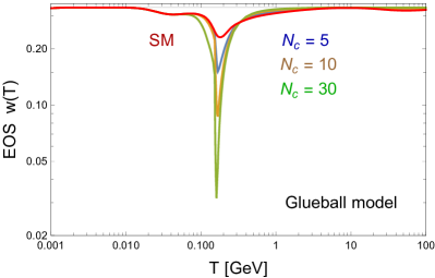
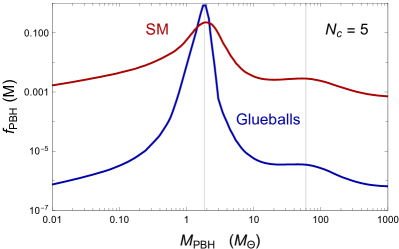
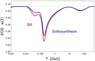
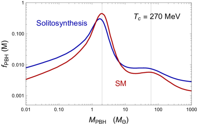
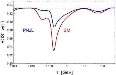
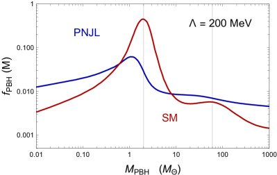
Figure 6: The equation of state around the phase transition, as a function of the temperature of the Universe, and the PBH mass fraction distribution as a function of BH mass in solar units.

A rapid change in the equation of state of the plasma during the QCD transition will decrease the radiation pressure and thus will allow for a few (horizon) domains to collapse to form primordial black holes Carr:2019kxo ; Garcia-Bellido:2019tvz ; Bodeker:2020stj . The sensitivity to the equation of state is exponential and thus a small change in radiation pressure can completely change the PBH mass spectrum. The threshold for gravitational collapse $\delta_{c}(w)$ is a function of the equation-of-state parameter $w(T)$, see Ref. Musco:2012au , so the thermal history of the Universe can induce pronounced features in the PBH mass function even for a uniform power spectrum of fluctuations. The reason being that, if the PBH form from Gaussian inhomogeneities with root-mean-square amplitude $\delta_{\rm rms}$, then the fraction of horizon patches undergoing collapse to PBH when the temperature of the Universe is $T$ should be Carr:2019kxo

$$\beta(M)\approx{\rm Erfc}\!\left[\frac{\delta_{c}\big{(}w[T(M)]\big{)}}{\sqrt{2}\,\delta_{\rm rms}(M)}\right]\,,$$ (30)

where the temperature is related to the PBH mass by $T\approx 200\,\sqrt{M_{\odot}/M\,}\;{\rm MeV}$. This shows that $\beta(M)$ is exponentially sensitive to $w(M)$. The present CDM fraction for PBHs of mass $M$ is then

$$f_{\rm PBH}(M)\equiv\frac{1}{\rho_{\rm CDM}}\frac{d\,\rho_{\rm PBH}(M)}{d\ln M}\approx\frac{2\Omega_{\rm M}}{\Omega_{\rm CDM}}\,\beta(M)\sqrt{\frac{M_{\rm eq}}{M}}\,,$$ (31)

where $M_{\rm eq}=2.8\times 10^{17}\,M_{\odot}$ is the horizon mass at matter-radiation equality and $\rho_{\rm CDM}$ is the CDM density. We have computed the change in EOS,

$$w_{i}(T)=\frac{p_{\rm SM}(T)+p_{i}(T)}{\rho_{\rm SM}(T)+\rho_{i}(T)}\,,$$ (32)

during the thermal evolution of the universe in the three cases discussed above: Glueballs, Solitosynthesis and the PNJL model. Each one gives a different mass spectrum for PBH, when taking into account the exponentially sensitive collapse to PBH as the radiation pressure varies accross the corresponding transitions. In the case of Glueballs, it generates for large $N_{c}$ a delta function of PBH at a particular scale, which is strongly constrained by astrophysical and cosmological observations. On the other hand, the Solitosynthesis model changes only very slightly the PBH mass spectrum from that of the SM. Finally, the PNJL model is sufficiently different from the SM that the search for signatures of differences in the mass spectrum will eventually be detected in the mass distribution of black holes from GW interferometers like LIGO/Virgo/KAGRA, as well as with current microlensing surveys like OGLE/GAIA and future surveys like LSST.

To test the robustness of our PBH results, we changed the value of the critical temperature $T_{c}$ and the scale $\Lambda$ to lower values (but still above the BBN scale), in order to generate peaks at higher masses, and we found no significant differences with the curves shown in Fig. 6, which makes these mass spectra rather robust.

6 Conclusions

In this paper, we have discussed the potential of a stochastic gravitational wave background detection at Gaia or future THEIA mission to probe early universe physics. These astrometric surveys open up a new frequency window of gravitational wave detection between LISA and pulsar timing arrays. We pointed out that there are many scenarios of phase transitions associated with dark matter such as SIMP or asymmetric dark matter, solitosynthesis, cosmic defects, and primordial black holes that can lead to detectable signals. Uncertainties in theoretical predictions are spelled out. We hope our work stimulates further discussions for the design of the missions and survey strategy in order to capture exciting physics potential.

Appendix A Low energy effective models for modeling confinement transitions

A.1 Linear sigma model

For convenience we give just the details of the potential for four light flavours

$$V(\phi,T)=V_{0}(\phi)+V_{T}(\phi,T)$$ (33)

where

$$V_{0}(\phi) = \frac{1}{32}\left(-16m_{\sigma}^{2}\phi^{2}+(\kappa+4\lambda-\mu_{\sigma})\phi^{4}\right)$$ (34)

$$V_{T}(\phi,T) = \bar{J}_{B}(m_{\phi}^{2}/T^{2})+\bar{J}_{B}(m_{\eta}^{2}/T^{2})+15\bar{J}_{B}(m_{X_{8}}^{2}/T^{2})+8\bar{J}_{B}(m_{X_{3}}^{2}/T^{2})+15\bar{J}_{B}(m_{\pi_{8}}^{2}/T^{2})$$ (35)

$$+8\bar{J}_{B}(m_{\pi_{3}}^{2}/T^{2})+\bar{J}_{B}(m_{\eta_{\psi}})+\bar{J}_{B}(m_{\eta_{\chi}}^{2}/T^{2}).$$

In the above

$$\bar{J}_{B}(z^{2})=\frac{T^{4}}{2\pi^{2}}\int_{0}^{\infty}dxx^{2}\log\left[1-e^{\sqrt{x^{2}+z^{2}}}\right]-\frac{T}{12\pi}\left((z^{2}+\frac{1}{12}(3\kappa+17\lambda)T^{2})^{3/2})-z^{3}\right)$$ (36)

and the masses are

$$m_{\phi} = \frac{1}{24}\left(9\kappa\phi^{2}+36\lambda\phi^{2}-9\mu\phi^{2}+6\mu_{s}-24m_{\Sigma}\right)$$ (37)

$$m_{\eta} = \frac{1}{8}\left(\phi^{2}[\kappa+4\lambda+3\mu]+2\mu\sigma\right)-m_{\Sigma}$$ (38)

$$m_{X_{8}} = \frac{1}{8}\phi^{2}\left(3\kappa+4\lambda+\mu\right)-m_{\Sigma}$$ (39)

$$m_{X_{3}} = \frac{1}{24}\left(9\kappa\phi^{2}+12\lambda\phi^{2}+3\mu\phi^{2}-24m_{\Sigma}\right)$$ (40)

$$m_{\pi_{8}} = \frac{1}{8}\phi^{2}\left(\kappa+4\lambda-\mu\right)-m_{\Sigma}$$ (41)

$$m_{\pi_{3}} = \frac{1}{24}\left(3\kappa\phi^{2}+12\lambda\phi^{2}-3\mu\phi^{2}-24\mu._{\Sigma}\right)$$ (42)

$$m_{\eta_{\psi}} = \frac{1}{24}\left(3\phi^{2}[3\kappa+4\lambda+\mu]+18\mu_{s}-24\mu_{\Sigma}\right)$$ (43)

$$m_{\eta_{\chi}} = \frac{1}{24}\left(3\phi^{2}[\kappa+4\lambda-\mu]+18\mu_{S}-24m_{\Sigma}\right)$$ (44)

A.2 (p)NJL model

The effective potential for the composite field, $\sigma$, in both the NJL and PNJL model is as follows

$$V_{\rm eff}^{\rm(P)NJL}(\bar{\sigma},L,T)=V_{0}^{\rm(P)NJL}(\bar{\sigma})+V_{\rm CW}^{\rm(P)NJL}(\bar{\sigma})+V_{\rm FT}^{\rm(P)NJL}(\bar{\sigma},L,T)$$ (45)

where

$$V_{0}^{\rm(P)NJL}(\bar{\sigma}) = \frac{3}{8G}\bar{\sigma}^{2}-\frac{G_{D}}{16G^{3}}\bar{\sigma}^{3}$$ (46)

$$V_{\rm CW}^{\rm(P)NJL}(\bar{\sigma}) = -\frac{3N_{C}}{16\pi^{2}}\left[\Lambda^{4}\log\left(1+\frac{M^{2}}{\Lambda^{2}}\right)-M^{4}\log\left(1+\frac{\Lambda^{2}}{M^{2}}\right)+\Lambda^{2}M^{2}\right]$$ (47)

$$V_{\rm FT}^{\rm(P)NJL} = -\frac{6T^{2}}{\pi^{2}}\int_{0}^{\infty}dxx^{2}\log\left(1+e^{-3\sqrt{x^{2}+r^{2}}}+3Le^{-\sqrt{x^{2}+r^{2}}}+3Le^{-2\sqrt{x^{2}+r^{2}}}\right)$$ (48)

$$+T^{4}\left(-\frac{1}{2}a(T)L^{2}+b(T)\log[1-6L^{2}-3L^{4}+8L^{3}]\right).$$

The last term is the potential for the glueballs and exists only in the pNJL model where the log term is from the Haar measure. We follow the strategy of ref Helmboldt:2019pan in minimizing the potential with respect to $L$, for each value of $\bar{\sigma}$ to reduce the problem to a single field problem. One can choose coefficients such that the potential reproduces the surface tension and the evolution of the pressure for $N_{C}=3$

$$a(T) = a_{0}+a_{1}\frac{T_{C}}{T}+a_{2}\left(\frac{T_{C}}{T}\right)^{2}$$ (49)

$$b(T) = b_{3}\left(\frac{T_{C}}{T}\right)^{3}\ ,$$ (50)

where

$$a_{0}=3.51,\quad a_{1}=-2.47,\quad a_{2}=15.2,\quad b_{3}=-1.75.$$ (51)

In the above $T_{C}$ is an input parameter that needs to match the critical temperature of the potential. For each value of $G$ and $G_{D}$, one can iteratively modify $T_{C}$ until it matches the physical critical temperature. Finally the field dependent mass is

$$M=\bar{\sigma}-\frac{G_{D}}{8G^{2}}\bar{\sigma}^{2}.$$ (52)

The field $\bar{\sigma}$ is composite, thus the Euclidean action has a non-canonical kinetic term

$$S_{3}[\bar{\sigma}]=4\pi\int r^{2}dr\left[\frac{Z_{\sigma}^{-1}}{2}\left(\frac{d\bar{\sigma}}{dr}\right)^{2}+V_{\rm eff}(\bar{\sigma})\right]$$ (53)

where

$$Z_{\sigma}^{-1}=-3N_{C}\left(1-\frac{G_{D}}{4G^{2}}\sigma\right)^{2}\left[-2A_{0}+2B_{0}+8C_{0}-2\ell_{A}(r)+2\ell_{B}(r)+8\ell_{C}(r)\right]\ .$$ (54)

In the above $r=|M(\bar{\sigma})|/T$ with

$$A_{0} = \frac{1}{16\pi^{2}}\left[\log\left(1+\frac{\Lambda^{2}}{M^{2}}\right)-\frac{\Lambda^{2}}{\Lambda^{2}+M^{2}}\right]$$ (55)

$$B_{0} = -\frac{1}{32\pi^{2}}\frac{\Lambda^{4}}{(M^{2}+\Lambda^{2})^{2}}$$ (56)

$$C_{0} = \frac{1}{96\pi^{2}}\frac{3M^{2}\Lambda^{4}+\Lambda^{6}}{(M^{2}+\Lambda^{2})^{3}}$$ (57)

finally the relevant thermal integrals are

$$\ell_{A}(r) = -\frac{1}{4\pi^{2}}\int_{0}^{\infty}\left(\frac{x^{2}}{\left(x^{2}+r^{2}\right)^{3/2}}\frac{1}{1+{\rm exp}[\sqrt{x^{2}+r^{2}}]}\right.$$ (58)

$$+\frac{1}{2}\frac{x^{2}}{x^{2}+r^{2}}\frac{1}{1+\cosh[\sqrt{x^{2}+r^{2}}]}$$

$$\ell_{B}(r) = \frac{r^{2}}{16\pi^{2}}\int_{0}^{\infty}dx\left(\frac{3x^{2}}{(x^{2}+r^{2})^{5/2}}\frac{1}{1+\exp[\sqrt{x^{2}+r^{2}}]}+\frac{3x^{2}}{2(x^{2}+r^{2})^{2}}\frac{1}{1+\cosh\sqrt{[x^{2}+r^{2}]}}\right.$$ (59)

$$\left.+\frac{x^{2}}{2(x^{2}+r^{2})^{5/2}}\frac{1}{1+\cosh[\sqrt{x^{2}+r^{2}}]}\right)$$

$$\ell_{C}(r) = -\frac{r^{4}}{96pi^{2}}\int_{0}^{\infty}dx\left(\frac{15x^{2}}{2(x^{2}+r^{2})^{7/2}}\frac{1}{1+\exp[\sqrt{x^{2}+r^{2}}]}+\frac{15x^{2}}{2(x^{2}+r^{2})^{3}}\frac{1}{1+\cosh[\sqrt{x^{2}+r^{2}}]}\right.$$ (60)

$$\left.\frac{3x^{2}}{(x^{2}+r^{2})^{5/2}}\frac{\tanh(\frac{1}{2}\sqrt{r^{2}+x^{2}})}{1+\cosh[\sqrt{x^{2}+r^{2}}]}+\frac{x^{2}}{2(x^{2}+r^{2})^{2}}\frac{1}{1+\cosh[\sqrt{x^{2}+r^{2}}]}\right.$$

$$-\frac{3x^{2}}{2(x^{2}+r^{2})^{2}}\frac{1}{(1+\cosh\sqrt{x^{2}+r^{2}})^{2}}$$

References

- (1) Gaia Collaboration, A. G. A. Brown et al., “Gaia Data Release 2,” Astron. Astrophys. 616 (2018) A1, arXiv:1804.09365 [astro-ph.GA].
- (2) A. Vallenari, “The future of astrometry in space,” Frontiers in Astronomy and Space Sciences 5 (2018) 11. https://www.frontiersin.org/article/10.3389/fspas.2018.00011.
- (3) C. J. Moore, D. P. Mihaylov, A. Lasenby, and G. Gilmore, “Astrometric Search Method for Individually Resolvable Gravitational Wave Sources with Gaia,” Phys. Rev. Lett. 119 (2017) no. 26, 261102, arXiv:1707.06239 [astro-ph.IM].
- (4) D. P. Mihaylov, C. J. Moore, J. R. Gair, A. Lasenby, and G. Gilmore, “Astrometric Effects of Gravitational Wave Backgrounds with non-Einsteinian Polarizations,” Phys. Rev. D 97 (2018) no. 12, 124058, arXiv:1804.00660 [gr-qc].
- (5) D. P. Mihaylov, C. J. Moore, J. Gair, A. Lasenby, and G. Gilmore, “Astrometric effects of gravitational wave backgrounds with nonluminal propagation speeds,” Phys. Rev. D 101 (2020) no. 2, 024038, arXiv:1911.10356 [gr-qc].
- (6) L. G. Book and E. E. Flanagan, “Astrometric Effects of a Stochastic Gravitational Wave Background,” Phys. Rev. D 83 (2011) 024024, arXiv:1009.4192 [astro-ph.CO].
- (7) L. Lentati et al., “European Pulsar Timing Array Limits On An Isotropic Stochastic Gravitational-Wave Background,” Mon. Not. Roy. Astron. Soc. 453 (2015) no. 3, 2576–2598, arXiv:1504.03692 [astro-ph.CO].
- (8) NANOGrav Collaboration, Z. Arzoumanian et al., “The NANOGrav 12.5 yr Data Set: Search for an Isotropic Stochastic Gravitational-wave Background,” Astrophys. J. Lett. 905 (2020) no. 2, L34, arXiv:2009.04496 [astro-ph.HE].
- (9) N. Bartolo et al., “Science with the space-based interferometer LISA. IV: Probing inflation with gravitational waves,” JCAP 1612 (2016) 026, arXiv:1610.06481 [astro-ph.CO].
- (10) K. Schmitz, “New Sensitivity Curves for Gravitational-Wave Experiments,” arXiv:2002.04615 [hep-ph].
- (11) E. Thrane and J. D. Romano, “Sensitivity curves for searches for gravitational-wave backgrounds,” Phys. Rev. D 88 (2013) no. 12, 124032, arXiv:1310.5300 [astro-ph.IM].
- (12) R. van Haasteren et al., “Placing limits on the stochastic gravitational-wave background using European Pulsar Timing Array data,” Mon. Not. Roy. Astron. Soc. 414 (2011) no. 4, 3117–3128, arXiv:1103.0576 [astro-ph.CO]. [Erratum: Mon.Not.Roy.Astron.Soc. 425, 1597 (2012)].
- (13) G. Janssen et al., “Gravitational wave astronomy with the SKA,” PoS AASKA14 (2015) 037, arXiv:1501.00127 [astro-ph.IM].
- (14) T. J. W. Lazio, S. Bhaskaran, C. Cutler, W. M. Folkner, R. S. Park, J. A. Ellis, T. Ely, S. R. Taylor, and M. Vallisneri, “Solar System Ephemerides, Pulsar Timing, Gravitational Waves, \& Navigation,” IAU Symp. 337 (2017) 150–153, arXiv:1801.02898 [astro-ph.IM].
- (15) C. Caprini et al., “Detecting gravitational waves from cosmological phase transitions with LISA: an update,” JCAP 03 (2020) 024, arXiv:1910.13125 [astro-ph.CO].
- (16) K. Yagi and N. Seto, “Detector configuration of DECIGO/BBO and identification of cosmological neutron-star binaries,” Phys. Rev. D 83 (2011) 044011, arXiv:1101.3940 [astro-ph.CO]. [Erratum: Phys.Rev.D 95, 109901 (2017)].
- (17) S. Kawamura et al., “The Japanese space gravitational wave antenna DECIGO,” Class. Quant. Grav. 23 (2006) S125–S132.
- (18) S. Kawamura et al., “Current status of space gravitational wave antenna DECIGO and B-DECIGO,” arXiv:2006.13545 [gr-qc].
- (19) LIGO Scientific Collaboration, J. Aasi et al., “Advanced LIGO,” Class. Quant. Grav. 32 (2015) 074001, arXiv:1411.4547 [gr-qc].
- (20) M. Punturo et al., “The Einstein Telescope: A third-generation gravitational wave observatory,” Class. Quant. Grav. 27 (2010) 194002.
- (21) M. Hindmarsh, S. J. Huber, K. Rummukainen, and D. J. Weir, “Gravitational waves from the sound of a first order phase transition,” Phys. Rev. Lett. 112 (2014) 041301, arXiv:1304.2433 [hep-ph].
- (22) M. Hindmarsh, S. J. Huber, K. Rummukainen, and D. J. Weir, “Numerical simulations of acoustically generated gravitational waves at a first order phase transition,” Phys. Rev. D 92 (2015) no. 12, 123009, arXiv:1504.03291 [astro-ph.CO].
- (23) M. Hindmarsh, S. J. Huber, K. Rummukainen, and D. J. Weir, “Shape of the acoustic gravitational wave power spectrum from a first order phase transition,” Phys. Rev. D 96 (2017) no. 10, 103520, arXiv:1704.05871 [astro-ph.CO]. [Erratum: Phys.Rev.D 101, 089902 (2020)].
- (24) H.-K. Guo, K. Sinha, D. Vagie, and G. White, “Phase Transitions in an Expanding Universe: Stochastic Gravitational Waves in Standard and Non-Standard Histories,” arXiv:2007.08537 [hep-ph].
- (25) D. Cutting, M. Hindmarsh, and D. J. Weir, “Vorticity, kinetic energy, and suppressed gravitational wave production in strong first order phase transitions,” Phys. Rev. Lett. 125 (2020) no. 2, 021302, arXiv:1906.00480 [hep-ph].
- (26) F. Giese, T. Konstandin, K. Schmitz, and J. Van De Vis, “Model-independent energy budget for LISA,” JCAP 01 (2021) 072, arXiv:2010.09744 [astro-ph.CO].
- (27) F. Giese, T. Konstandin, and J. van de Vis, “Model-independent energy budget of cosmological first-order phase transitions—A sound argument to go beyond the bag model,” JCAP 07 (2020) no. 07, 057, arXiv:2004.06995 [astro-ph.CO].
- (28) H.-K. Guo, K. Sinha, D. Vagie, and G. White, “The Benefits of Diligence: How Precise are Predicted Gravitational Wave Spectra in Models with Phase Transitions?,” arXiv:2103.06933 [hep-ph].
- (29) Y. Hochberg, E. Kuflik, T. Volansky, and J. G. Wacker, “Mechanism for Thermal Relic Dark Matter of Strongly Interacting Massive Particles,” Phys. Rev. Lett. 113 (2014) 171301, arXiv:1402.5143 [hep-ph].
- (30) A. Bazavov et al., “The chiral and deconfinement aspects of the QCD transition,” Phys. Rev. D 85 (2012) 054503, arXiv:1111.1710 [hep-lat].
- (31) S. Gupta, X. Luo, B. Mohanty, H. G. Ritter, and N. Xu, “Scale for the Phase Diagram of Quantum Chromodynamics,” Science 332 (2011) 1525–1528, arXiv:1105.3934 [hep-ph].
- (32) M. Gell-Mann and M. Levy, “The axial vector current in beta decay,” Nuovo Cim. 16 (1960) 705.
- (33) Y. Nambu and G. Jona-Lasinio, “Dynamical Model of Elementary Particles Based on an Analogy with Superconductivity. 1.,” Phys. Rev. 122 (1961) 345–358.
- (34) Y. Nambu and G. Jona-Lasinio, “DYNAMICAL MODEL OF ELEMENTARY PARTICLES BASED ON AN ANALOGY WITH SUPERCONDUCTIVITY. II,” Phys. Rev. 124 (1961) 246–254.
- (35) K. Fukushima, “Chiral effective model with the Polyakov loop,” Phys. Lett. B 591 (2004) 277–284, arXiv:hep-ph/0310121.
- (36) D. Croon, O. Gould, P. Schicho, T. V. I. Tenkanen, and G. White, “Theoretical uncertainties for cosmological first-order phase transitions,” arXiv:2009.10080 [hep-ph].
- (37) R. D. Pisarski and F. Wilczek, “Remarks on the Chiral Phase Transition in Chromodynamics,” Phys. Rev. D 29 (1984) 338–341.
- (38) H. Davoudiasl, “LIGO/Virgo Black Holes from a First Order Quark Confinement Phase Transition,” Phys. Rev. Lett. 123 (2019) no. 10, 101102, arXiv:1902.07805 [hep-ph].
- (39) D. J. Schwarz and M. Stuke, “Lepton asymmetry and the cosmic QCD transition,” JCAP 11 (2009) 025, arXiv:0906.3434 [hep-ph]. [Erratum: JCAP 10, E01 (2010)].
- (40) G. Barenboim, W. H. Kinney, and W.-I. Park, “Resurrection of large lepton number asymmetries from neutrino flavor oscillations,” Phys. Rev. D 95 (2017) no. 4, 043506, arXiv:1609.01584 [hep-ph].
- (41) D. Croon, R. Houtz, and V. Sanz, “Dynamical Axions and Gravitational Waves,” JHEP 07 (2019) 146, arXiv:1904.10967 [hep-ph].
- (42) D. Croon, A. Kusenko, A. Mazumdar, and G. White, “Solitosynthesis and Gravitational Waves,” Phys. Rev. D 101 (2020) no. 8, 085010, arXiv:1910.09562 [hep-ph].
- (43) A. J. Helmboldt, J. Kubo, and S. van der Woude, “Observational prospects for gravitational waves from hidden or dark chiral phase transitions,” Phys. Rev. D 100 (2019) no. 5, 055025, arXiv:1904.07891 [hep-ph].
- (44) S. Roessner, C. Ratti, and W. Weise, “Polyakov loop, diquarks and the two-flavour phase diagram,” Phys. Rev. D 75 (2007) 034007, arXiv:hep-ph/0609281.
- (45) Y. Hochberg, E. Kuflik, and H. Murayama, “SIMP Spectroscopy,” JHEP 05 (2016) 090, arXiv:1512.07917 [hep-ph].
- (46) E. Kuflik, M. Perelstein, N. R.-L. Lorier, and Y.-D. Tsai, “Elastically Decoupling Dark Matter,” Phys. Rev. Lett. 116 (2016) no. 22, 221302, arXiv:1512.04545 [hep-ph].
- (47) A. Fradette, M. Pospelov, J. Pradler, and A. Ritz, “Cosmological Constraints on Very Dark Photons,” Phys. Rev. D 90 (2014) no. 3, 035022, arXiv:1407.0993 [hep-ph].
- (48) A. Kusenko, “Phase transitions precipitated by solitosynthesis,” Phys. Lett. B 406 (1997) 26–33, arXiv:hep-ph/9705361.
- (49) S. R. Coleman, “Q Balls,” Nucl. Phys. B 262 (1985) 263. [Erratum: Nucl.Phys.B 269, 744 (1986)].
- (50) M. Postma and G. White, “Cosmological phase transitions: is effective field theory just a toy?,” arXiv:2012.03953 [hep-ph].
- (51) B. Lucini, M. Teper, and U. Wenger, “Properties of the deconfining phase transition in SU(N) gauge theories,” JHEP 02 (2005) 033, arXiv:hep-lat/0502003.
- (52) S. Datta and S. Gupta, “Continuum Thermodynamics of the Gluo Plasma,” Phys. Rev. D 82 (2010) 114505, arXiv:1006.0938 [hep-lat].
- (53) M. Panero, “Thermodynamics of the QCD plasma and the large-N limit,” Phys. Rev. Lett. 103 (2009) 232001, arXiv:0907.3719 [hep-lat].
- (54) N. O. Agasian, M. S. Lukashov, and Y. A. Simonov, “Nonperturbative SU(3) thermodynamics and the phase transition,” Eur. Phys. J. A 53 (2017) no. 6, 138, arXiv:1701.07959 [hep-ph].
- (55) S. Borsanyi, G. Endrodi, Z. Fodor, S. D. Katz, and K. K. Szabo, “Precision SU(3) lattice thermodynamics for a large temperature range,” JHEP 07 (2012) 056, arXiv:1204.6184 [hep-lat].
- (56) W.-C. Huang, M. Reichert, F. Sannino, and Z.-W. Wang, “Testing the Dark Confined Landscape: From Lattice to Gravitational Waves,” arXiv:2012.11614 [hep-ph].
- (57) Z. Kang, S. Matsuzaki, and J. Zhu, “Dark Confinement-Deconfinement Phase Transition: A Roadmap from Polyakov Loop Models to Gravitational Waves,” arXiv:2101.03795 [hep-ph].
- (58) J. Halverson, C. Long, A. Maiti, B. Nelson, and G. Salinas, “Gravitational waves from dark Yang-Mills sectors,” arXiv:2012.04071 [hep-ph].
- (59) T. D. Cohen, S. Lawrence, and Y. Yamauchi, “Thermodynamics of large- QCD and the nature of metastable phases,” Phys. Rev. C 102 (2020) no. 6, 065206, arXiv:2006.14545 [hep-ph].
- (60) L. Bian, R.-G. Cai, J. Liu, X.-Y. Yang, and R. Zhou, “On the gravitational wave sources from the NANOGrav 12.5-yr data,” arXiv:2009.13893 [astro-ph.CO].
- (61) X.-L. Chen and M. Kamionkowski, “Particle decays during the cosmic dark ages,” Phys. Rev. D 70 (2004) 043502, arXiv:astro-ph/0310473.
- (62) Y. Yang, “Constraints on the basic parameters of dark matter using the Planck data,” Phys. Rev. D 91 (2015) no. 8, 083517, arXiv:1504.01195 [astro-ph.CO].
- (63) J. Coffey, L. Forestell, D. E. Morrissey, and G. White, “Cosmological Bounds on sub-GeV Dark Vector Bosons from Electromagnetic Energy Injection,” JHEP 07 (2020) 179, arXiv:2003.02273 [hep-ph].
- (64) L. Forestell, D. E. Morrissey, and K. Sigurdson, “Non-Abelian Dark Forces and the Relic Densities of Dark Glueballs,” Phys. Rev. D 95 (2017) no. 1, 015032, arXiv:1605.08048 [hep-ph].
- (65) L. Forestell, D. E. Morrissey, and K. Sigurdson, “Cosmological Bounds on Non-Abelian Dark Forces,” Phys. Rev. D 97 (2018) no. 7, 075029, arXiv:1710.06447 [hep-ph].
- (66) J. E. Juknevich, D. Melnikov, and M. J. Strassler, “A Pure-Glue Hidden Valley I. States and Decays,” JHEP 07 (2009) 055, arXiv:0903.0883 [hep-ph].
- (67) J. E. Juknevich, “Pure-glue hidden valleys through the Higgs portal,” JHEP 08 (2010) 121, arXiv:0911.5616 [hep-ph].
- (68) J. Ellis and M. Lewicki, “Cosmic String Interpretation of NANOGrav Pulsar Timing Data,” Phys. Rev. Lett. 126 (2021) no. 4, 041304, arXiv:2009.06555 [astro-ph.CO].
- (69) S. Blasi, V. Brdar, and K. Schmitz, “Has NANOGrav found first evidence for cosmic strings?,” Phys. Rev. Lett. 126 (2021) no. 4, 041305, arXiv:2009.06607 [astro-ph.CO].
- (70) S. Datta, A. Ghosal, and R. Samanta, “Baryogenesis from ultralight primordial black holes and strong gravitational waves,” arXiv:2012.14981 [hep-ph].
- (71) J. Chakrabortty, G. Lazarides, R. Maji, and Q. Shafi, “Primordial Monopoles and Strings, Inflation, and Gravity Waves,” JHEP 02 (2021) 114, arXiv:2011.01838 [hep-ph].
- (72) R. Samanta and S. Datta, “Gravitational wave complementarity and impact of NANOGrav data on gravitational leptogenesis: cosmic strings,” arXiv:2009.13452 [hep-ph].
- (73) S. F. King, S. Pascoli, J. Turner, and Y.-L. Zhou, “Gravitational Waves and Proton Decay: Complementary Windows into Grand Unified Theories,” Phys. Rev. Lett. 126 (2021) no. 2, 021802, arXiv:2005.13549 [hep-ph].
- (74) W. Buchmuller, V. Domcke, and K. Schmitz, “From NANOGrav to LIGO with metastable cosmic strings,” Phys. Lett. B 811 (2020) 135914, arXiv:2009.10649 [astro-ph.CO].
- (75) N. Craig, I. Garcia Garcia, G. Koszegi, and A. McCune, “P not PQ,” arXiv:2012.13416 [hep-ph].
- (76) A. Brandenburg, E. Clarke, Y. He, and T. Kahniashvili, “Can we observe the QCD phase transition-generated gravitational waves through pulsar timing arrays?,” arXiv:2102.12428 [astro-ph.CO].
- (77) S.-L. Li, L. Shao, P. Wu, and H. Yu, “NANOGrav Signal from First-Order Confinement/Deconfinement Phase Transition in Different QCD Matters,” arXiv:2101.08012 [astro-ph.CO].
- (78) M. Lewicki and V. Vaskonen, “Gravitational waves from colliding vacuum bubbles in gauge theories,” arXiv:2012.07826 [astro-ph.CO].
- (79) A. Neronov, A. Roper Pol, C. Caprini, and D. Semikoz, “NANOGrav signal from magnetohydrodynamic turbulence at the QCD phase transition in the early Universe,” Phys. Rev. D 103 (2021) no. 4, 041302, arXiv:2009.14174 [astro-ph.CO].
- (80) Y. Nakai, M. Suzuki, F. Takahashi, and M. Yamada, “Gravitational Waves and Dark Radiation from Dark Phase Transition: Connecting NANOGrav Pulsar Timing Data and Hubble Tension,” arXiv:2009.09754 [astro-ph.CO].
- (81) A. Addazi, Y.-F. Cai, Q. Gan, A. Marciano, and K. Zeng, “NANOGrav results and Dark First Order Phase Transitions,” arXiv:2009.10327 [hep-ph].
- (82) K. Kohri and T. Terada, “Solar-Mass Primordial Black Holes Explain NANOGrav Hint of Gravitational Waves,” Phys. Lett. B 813 (2021) 136040, arXiv:2009.11853 [astro-ph.CO].
- (83) G. Domènech and S. Pi, “NANOGrav Hints on Planet-Mass Primordial Black Holes,” arXiv:2010.03976 [astro-ph.CO].
- (84) S. Sugiyama, V. Takhistov, E. Vitagliano, A. Kusenko, M. Sasaki, and M. Takada, “Testing Stochastic Gravitational Wave Signals from Primordial Black Holes with Optical Telescopes,” Phys. Lett. B 814 (2021) 136097, arXiv:2010.02189 [astro-ph.CO].
- (85) V. De Luca, G. Franciolini, and A. Riotto, “NANOGrav Data Hints at Primordial Black Holes as Dark Matter,” Phys. Rev. Lett. 126 (2021) no. 4, 041303, arXiv:2009.08268 [astro-ph.CO].
- (86) C. J. A. P. Martins and E. P. S. Shellard, “String evolution with friction,” Phys. Rev. D 53 (1996) 575–579, arXiv:hep-ph/9507335.
- (87) C. J. A. P. Martins and E. P. S. Shellard, “Quantitative string evolution,” Phys. Rev. D 54 (1996) 2535–2556, arXiv:hep-ph/9602271.
- (88) C. J. A. P. Martins and E. P. S. Shellard, “Extending the velocity dependent one scale string evolution model,” Phys. Rev. D 65 (2002) 043514, arXiv:hep-ph/0003298.
- (89) J. J. Blanco-Pillado, K. D. Olum, and B. Shlaer, “The number of cosmic string loops,” Phys. Rev. D 89 (2014) no. 2, 023512, arXiv:1309.6637 [astro-ph.CO].
- (90) J. J. Blanco-Pillado and K. D. Olum, “Stochastic gravitational wave background from smoothed cosmic string loops,” Phys. Rev. D 96 (2017) no. 10, 104046, arXiv:1709.02693 [astro-ph.CO].
- (91) T. Hiramatsu, M. Kawasaki, and K. Saikawa, “On the estimation of gravitational wave spectrum from cosmic domain walls,” JCAP 02 (2014) 031, arXiv:1309.5001 [astro-ph.CO].
- (92) K. Kadota, M. Kawasaki, and K. Saikawa, “Gravitational waves from domain walls in the next-to-minimal supersymmetric standard model,” JCAP 10 (2015) 041, arXiv:1503.06998 [hep-ph].
- (93) R. Zhou, J. Yang, and L. Bian, “Gravitational Waves from first-order phase transition and domain wall,” JHEP 04 (2020) 071, arXiv:2001.04741 [hep-ph].
- (94) T. Opferkuch, P. Schwaller, and B. A. Stefanek, “Ricci Reheating,” JCAP 07 (2019) 016, arXiv:1905.06823 [gr-qc].
- (95) B. Carr, S. Clesse, J. García-Bellido, and F. Kühnel, “Cosmic conundra explained by thermal history and primordial black holes,” Phys. Dark Univ. 31 (2021) 100755, arXiv:1906.08217 [astro-ph.CO].
- (96) J. García-Bellido, “Primordial black holes and the origin of the matter–antimatter asymmetry,” Phil. Trans. Roy. Soc. Lond. A377 (2019) no. 2161, 20190091.
- (97) D. Bodeker, F. Kühnel, I. M. Oldengott, and D. J. Schwarz, “Lepton Flavour Asymmetries and the Mass Spectrum of Primordial Black Holes,” arXiv:2011.07283 [astro-ph.CO].
- (98) I. Musco and J. C. Miller, “Primordial black hole formation in the early universe: critical behaviour and self-similarity,” Class. Quant. Grav. 30 (2013) 145009, arXiv:1201.2379 [gr-qc].