Structure, size and statistical properties of chaotic components in a mixed-type Hamiltonian system

Abstract

We preform a detailed study of the chaotic component in mixed-type Hamiltonian systems on the example of a family of billiards (introduced by Robnik 1983). The phase space is divided into a grid of cells and a chaotic orbit is iterated a large number of times. The structure of the chaotic component is discerned from the cells visited by the chaotic orbit. The fractal dimension of the border of the chaotic component for various values of the billiard shape parameter is determined with the box counting method. The cell filling dynamics is compared to a model of uncorrelated motion the so-called random model (Robnik et. al. 1997) and deviations attributed to sticky objects in the phase space are found. The statistics of the number of orbit visits to the cells is analyzed and found to be in agreement with the random model in the long run. The stickiness of the various structures in the phase space is quantified in terms of the cell recurrence times. The recurrence time distributions in a few selected cells as well as the mean and standard deviation of recurrence times for all cells are analyzed. The standard deviation of cell recurrence time is found to be a good quantifier of stickiness on a global scale. Three methods for determining the measure of the chaotic component are compared and the measure is calculated for various values of the billiard shape parameter. Lastly, the decay of correlations and the diffusion of momenta is analyzed.

I Introduction

Generic Hamiltonian systems are typically neither integrable nor fully chaotic, but exhibit both regular and chaotic motion depending on the initial condition. The phase space is divided into several invariant components where the dynamics is regular on some and chaotic on others. The structure of the chaotic component in such mixed-type systems may be very complex, with the chaotic sea enveloping multitudes of KAM islands. The islands influence the dynamics of the chaotic orbits in their vicinity. Chaotic orbits that come close to a KAM island may spend extended periods of time in its vicinity in quasi regular motion, a phenomenon known as stickiness (Refs. [Bunimovich and Vela-Arevalo, 2012] and [Contopoulus and Harsoula, 2010] provide a good introduction to the topic). Additionally, cantori (MacKay et al., 1984; Mackay et al., 1984), i.e. the fractal remains of destroyed invariant tori, may also be present in the chaotic sea, acting as barriers to the chaotic dynamics. These types of intermittent behavior in Hamiltonian systems with mixed phase space may lead to the dynamics being only weakly chaotic in the sense that time correlations as well as recurrence time distributions decay more slowly (Chirikov and Shepelyansky, 1984, 1999; Vivaldi et al., 1983; Zaslavsky, 2002; Cristadoro and Ketzmerick, 2008; Abud and de Carvalho, 2013), non-exponentially as opposed to the exponential decay in some chaotic systems with strong mixing properties (Young, 1998, 1999; Hirata et al., 1999). It is however important to stress that a divided phase space is not a prerequisite for slow decay of correlation. An example of an ergodic K-system with power law decay of correlations is the stadium billiard (Bunimovich, 1979; Markarian, 2004). There the slow decay of correlations has been linked to the presence of sticky bouncing ball and boundary glancing orbits (Vivaldi et al., 1983).

Both the complexity of the phase space and the intermittent behavior of the orbits pose a challenge to determining the size or relative measure of a chaotic component. The typical island around island structures lead to a fractal border of the chaotic component. Determining the measure of the chaotic component to a high degree of accuracy may thus require very detailed phase portraits. These are usually obtained by iterating a chaotic orbit and letting it explore all of the available phase space. The problem is that the orbits may become frequently trapped by sticky objects and a large number of iterations may be needed to fully resolve the phase portrait. Cantori may also limit the accessibility to some parts of the chaotic component.

The need to accurately determine the measure of the chaotic component was motivated by the study of energy level statistics in the context of quantum chaos in generic autonomous Hamiltonian systems. In the strict semiclassical limit it is possible to separate chaotic eigenstates from regular ones (see Refs. (Percival, 1973; Berry, 1977; Voros, 1979; Shnirelman, 1979; Berry and Robnik, 1984; Robnik, 1998; Veble et al., 1999; Batistić and Robnik, 2010, 2013a, 2013b; Batistić et al., 2018) and references therein). The full spectrum can then be decomposed as a linear superposition of the chaotic and regular spectrum. The relative size of each component is given by the relative measure of the component in the classical phase space. An accurate value for the size of the chaotic component in the equivalent classical system is therefore vital in analyzing the spectral statistics of mixed-type quantum systems in the semiclassical limit.

The main goal of this paper is to present a method of determining the measure of the largest chaotic component in a mixed-type system, using as an example the family of billiards introduced in Ref. [Robnik, 1983]. The method involves dividing the phase space into a grid of cells and counting the visits of a chaotic orbit in each of the cells. The statistics of the orbit visits is then analyzed and compared to a model of completely uncorrelated random motion. If the cells dividing the phase space are sufficiently small and the number of orbit iterations suficiently large to reach the ergodic limit, the measure of the chaotic component can be extracted with a high degree of accuracy.

The paper is organized as follows. In Sec. II we define the family of billiards studied and describe some of the features of their phase spaces. We also describe the division of the phase space into cells. In Sec. III we estimate the fractal dimension for various billiards belonging to the aforementioned family. In Sec. IV we analyze the filling of the cells with regard to the number of orbit iterations as well as the statistics of the number of cell visitations and compare them with a model of completely uncorrelated motion. In Sec.V we analyze the cell recurrence times and their statistics. In Sec. VI we compare three methods of determining the measure of the chaotic component and discuss the connection to quantum chaos. In Sec. VII we examine the momentum autocorrelation function and the momentum diffusion. In Sec. VIII the results are discussed and concluded.

II The structure of the chaotic components

As an example of a mixed-type system we chose to study the family of billiards introduced in Ref. [Robnik, 1983]. The border of the billiard can be described in the complex plane as a smooth conformal mapping of the unit circle $|z|=1,$

$$z\rightarrow z+\lambda z^{2},$$ (1)

where the shape parameter is a real number $\lambda\in\left[0,\,0.5\right]$. The billiard border is a circle at $\lambda=0$ and thus integrable. It has been proven that in the other extreme case $\lambda=0.5$ the billiard is an ergodic K-system (Markarian, 1993). Between both extremes the phase space is mixed containing both chaotic and regular components. The shape of the border is convex up to $\lambda=0.25$ and concave for larger values of the shape parameter. The phase space is defined by the Poincaré-Birkhoff coordinates $\left(s,\,p\right)$, where $s$ is the arc-length of the billiard boundary in the counterclockwise direction measured from the point where it intersects the real axis, and the momentum is the sine of the reflection angle of the particle $p=\sin\alpha$. The phase space is thus a cylinder $x=\left(s,\,p\right)\in\left[0,\,\mathcal{L}\right]\times\left[-1,\,1\right]$, where we take $s$ to be periodic with a period equal to the total length of the billiard boundary

$$\mathcal{L}=\int_{0}^{2\pi}\mathrm{d}\varphi\sqrt{1+4\lambda^{2}+4\lambda\cos\varphi}.$$ (2)

The billiard map, mapping the successive collisions, is area preserving (Berry, 1981). In Fig. 1 we show a chaotic orbit in a small region of the phase space for the $\lambda=0.135$ billiard. The shade of gray denotes the number of times the orbit has visited. Unvisited areas are depicted in white. Because of the multitude of KAM islands of stability, the chaotic component has a complex fractal structure as is typical for mixed-type Hamiltonian systems. The borders of the islands can also represent sticky objects. The chaotic orbit tends to stick to the area around an island for an extended number of bounces. We may also see larger areas of a mostly uniform shade distinct from those of other areas, most notably on the upper border of the chaotic component. This indicates the presence of cantori, the remnants of the destroyed invariant KAM tori, that act as barriers for the orbit. Another notable feature of strictly convex billiards as is the case for $\lambda<0.25$ is the presence of Lazutkin caustics (Lazutkin, 1973). A curve is called a caustic of a billiard when, if some link of a trajectory (by link we mean the straight segment of the trajectory between two consecutive bounces) is tangent to the curve, then all other links of the same trajectory are tangent to this curve. The Lazutkin caustic is manifested in the phase space as a Lazutkin torus. The Lazutkin tori limit the area accessible to the chaotic component near the upper and lower border of the phase space. In Fig. 1 the torus is reached at $p\approx 0.9.$ We note that at the shape parameter value $\lambda=0.25$ the Lazutkin tori are destroyed (Mather, 1982) because a point with zero curvature exists on the billiard border at $s=\frac{\mathcal{L}}{2}$, $z=-1$.

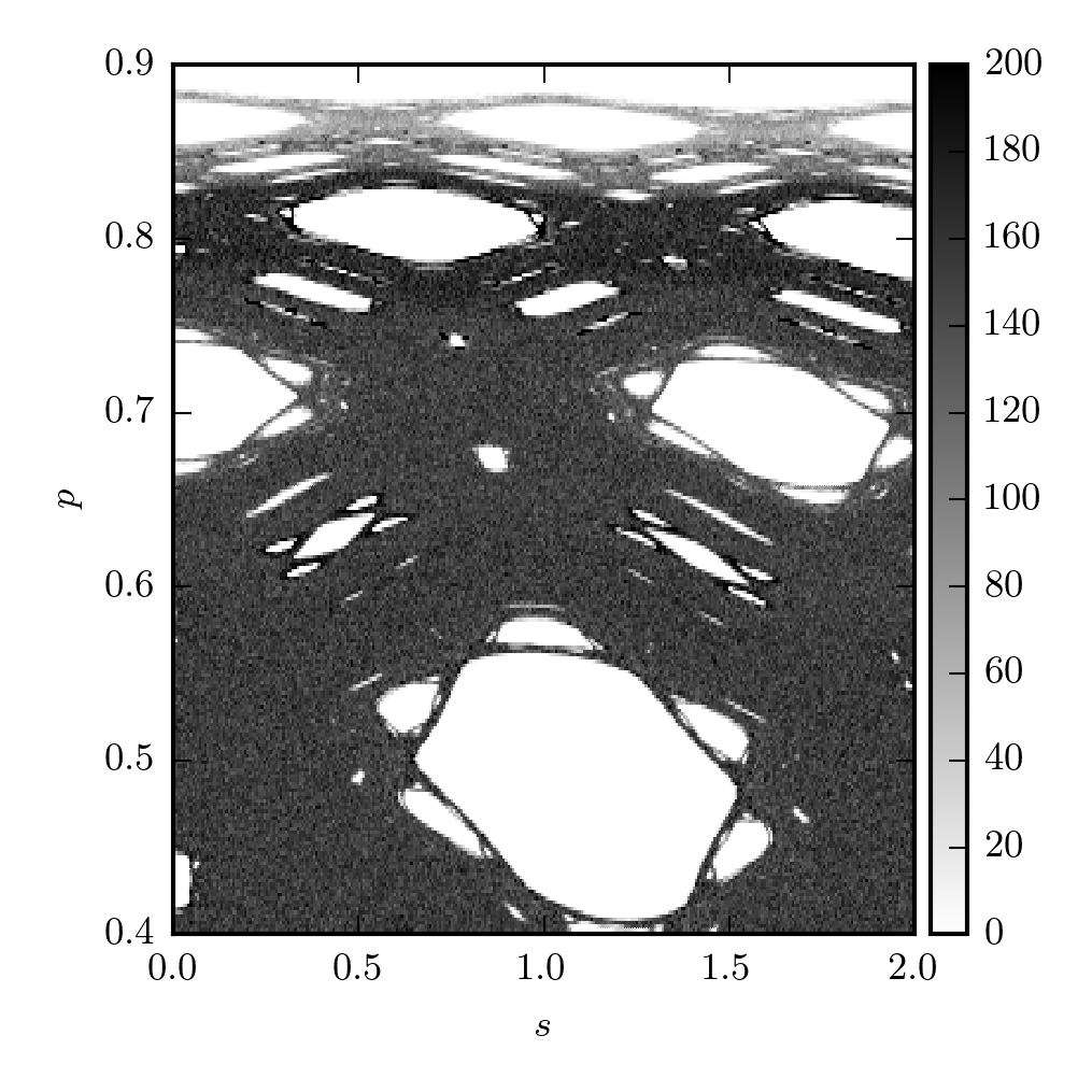
Figure 1: Part of the phase space visited by a single chaotic orbit in the billiard defined by Eq. (1) for $\lambda=0.135$. The number of visits is represented by the lightness of the plot.

We will concentrate our analysis on the billiards with a single dominant chaotic component much larger in size than the other chaotic components. In terms of the shape parameter this means $\lambda\geq 0.1175$. For lower values multiple small chaotic components form around the unstable periodic orbits and are separated by invariant tori. These are comparable in size and each represents only a small fraction of the entire phase space. At $\lambda\approx 0.1175$ most of the tori are destroyed and several chaotic components merge into a single larger one. To confirm that the orbits in these areas of phase space are indeed chaotic we determined the Lyapunov exponent. Let $\delta x\left(T\right)$ be the separation of two orbits at $T$ iterations and $\delta x_{0}$ the initial separation. The Lyapunov exponent is then

$$\varLambda=\lim_{T\rightarrow\infty}\lim_{\delta x_{0}\rightarrow 0}\frac{1}{T}\ln\frac{\left|\delta x\left(T\right)\right|}{\left|\delta x_{0}\right|}.$$ (3)

The Lyapunov exponent on the largest chaotic component as a function of the shape parameter, determined by the method introduced in Ref. (Benettin et al., 1976), is presented in Fig. 2.

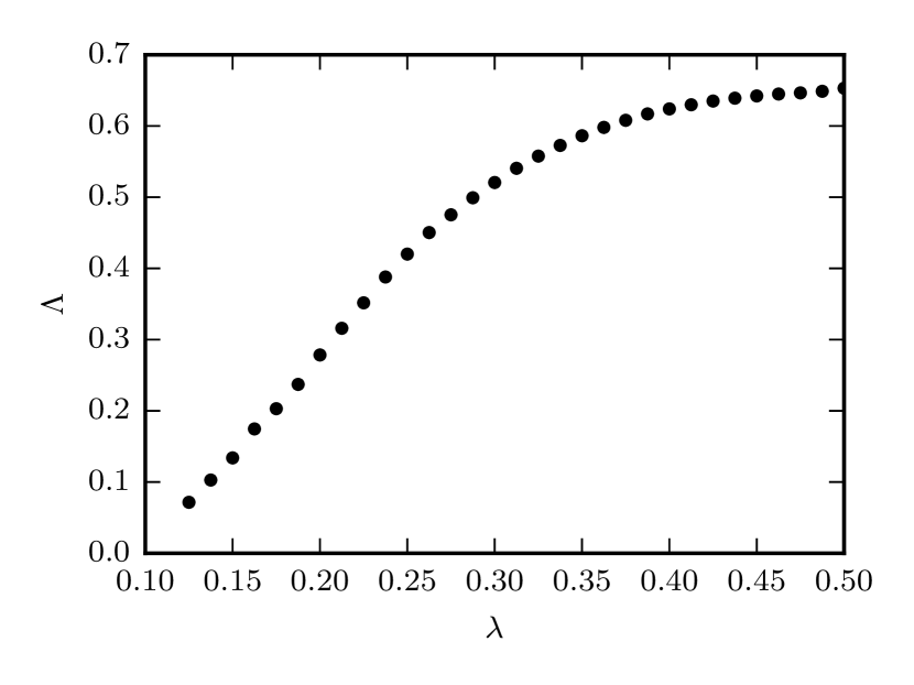
Figure 2: Lyapunov exponent on the largest chaotic component as a function of the shape parameter.

In Fig. 3 we show the area of phase space occupied by the largest chaotic component for various values of the shape parameter. At $\lambda=0.135$ the accessible phase space is still significantly limited by the Lazutkin tori in addition to the large number of stable islands. When $\lambda$ is increased the tori are moved ever further towards the border of the phase space, until finally disappearing at $\lambda=0.25$. Furthermore, the billiards become increasingly chaotic with more and more of the stable islands being destroyed until only some tiny islands remain at $\lambda=0.25$. At $\lambda=0.5$ the billiard is rigorously proven to be ergodic (Markarian, 1993). The question arises: At a given shape what proportion of the phase space is filled by the chaotic component? The complexity of the structure of the phase space as well as the presence of sticky objects pose significant obstacles in answering this question. Because the border of the chaotic component is fractal it is difficult to decide whether an area on the border of the phase space still belongs to the chaotic component or not. Chaotic orbits may also become trapped by sticky objects and cantori and may need a very large number of iterations to explore all of the available phase space.

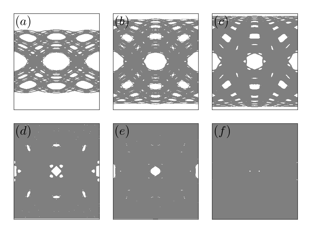
Figure 3: Portraits of the largest chaotic component in the phase space cylinder$\left(s,\,p\right)$ for different values of the shape parameter $\lambda$. (a) $\lambda=0.1175$, (b) $\lambda=0.135$, (c) $\lambda=0.15$, (d) $\lambda=0.18$, (e) $\lambda=0.2$, (f) $\lambda=0.25$. The gray area represents the chaotic component.

To determine the sizes of the chaotic components we improved the procedure from Ref. [Dobnikar, 1996]. The phase space is partitioned on a rectangular grid into $L\times L$ cells. We then select an initial condition in the largest chaotic component of the billiard and iterate the orbit for a large number of bounces $T$. We monitor which of the cells are visited by the chaotic orbit to determine whether the portion of the phase space contained in the cell is a part of the chaotic component or not. We will refer to cells that are never visited by the chaotic orbit as empty cells and cells that are visited as filled cells.

III Fractal dimension of the boundary

To measure the complexity of the boundary of the chaotic component we calculated its fractal dimension (Ott, 2002) using the box-counting method. To determine the fractal dimension of a set, we cover the set with boxes of some side length $\epsilon$. Let $N_{B}\left(\epsilon\right)$ be the number of boxes needed to cover the set at a given $\epsilon$. The box-counting dimension is

$$D=\underset{\epsilon\rightarrow 0}{\lim}\frac{\log N_{B}\left(\epsilon\right)}{\log\left(\frac{1}{\epsilon}\right)}.$$ (4)

In the case of our billiards we use the phase space cells as defined above for the boxes. The side length of a cell is proportional to the inverse of the grid size $\epsilon\propto\frac{1}{L}$. We refer to cells that are filled but have at least one empty neighboring cell as border cells. The orbit visited a border cell at least once, meaning at least some of the phase space contained in it is part of the chaotic component. However, it is likely that the whole cell is not filled by the chaotic component because the neighboring cells are empty. The border of the chaotic component is thus covered by the border cells. From the definition (4) we derive the following relation for the number of border cells $\log N_{B}=D\log L+\mathrm{const}.$ We can determine the fractal dimension by counting the number of border cells at various grid sizes and fitting the data with a line.

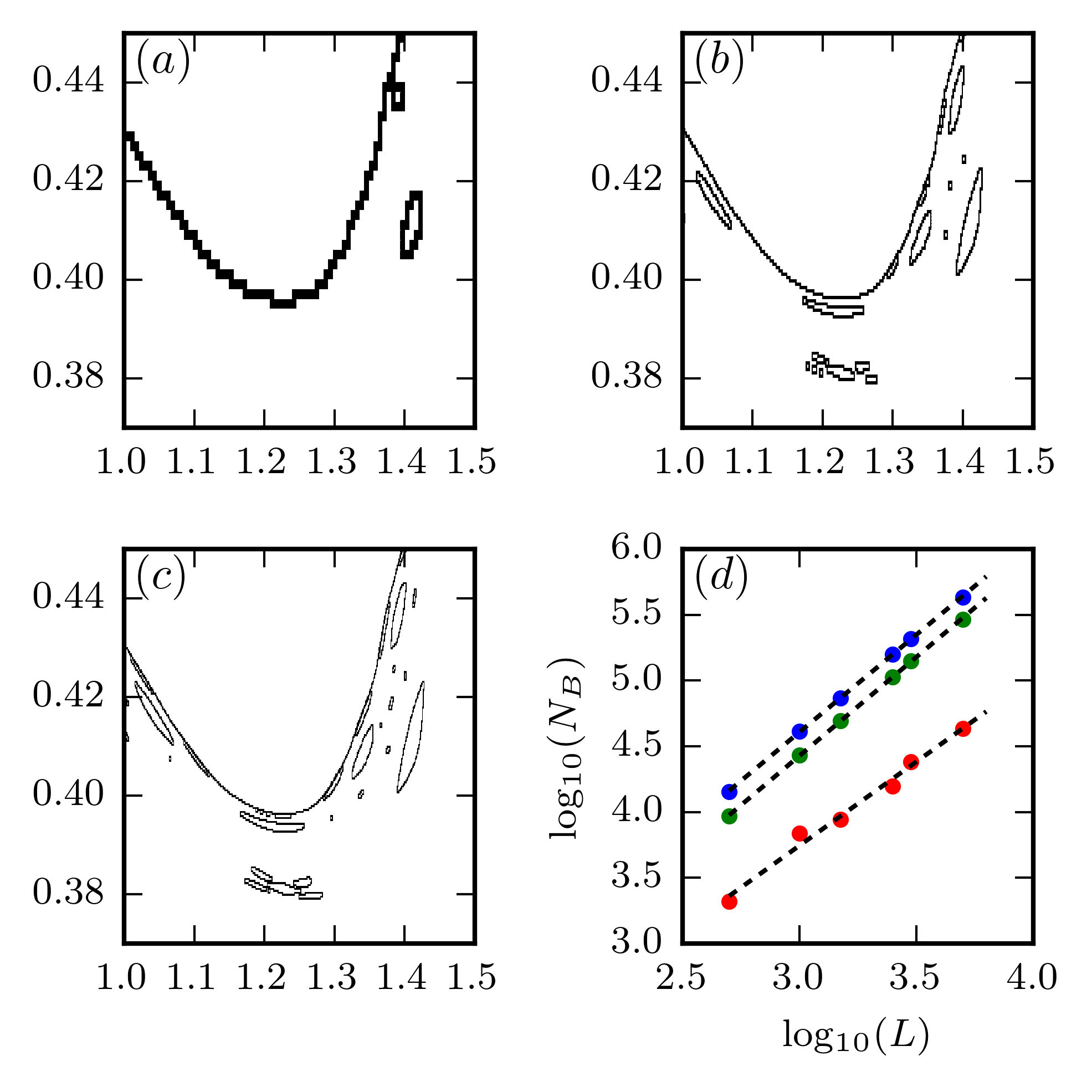
Figure 4: Plots showing the border cells of the largest chaotic component in the vicinity of a stable island in the $\lambda=0.15$ billiard at various grid sizes (a) $L=1000$, (b) $L=3000$ and (c) $L=5000$. Panel (d) shows the logarithm of the number of border cells versus the logarithm of the grid size for three different values of $\lambda$. From top to bottom (blue) $\lambda=0.1175$, (green) $\lambda=0.15$ and (red) $\lambda=0.2$. The slope of the line is the estimate for the fractal dimension.

In determining the fractal dimension we used cell grids between $L=500$ and $L=5000$. The number of orbit iterations was $T=10^{11}$ ensuring a large number of iterations per cell even for the largest grid size. In Fig. 4 (a-c) we show the border cells for a small area of phase space near one of the islands around the stable period three orbit of the $\lambda=0.15$ billiard. As the cells get smaller more and more details of the structure of the border of the chaotic component may be discerned. The logarithm of the number of border cells versus the logarithm of the grid size for three different values of $\lambda$ is shown on panel (d) of the same figure. We fit the data with a least squares linear regression model. The slope of the line is the fractal dimension $D$. The values of the fractal dimension along with an error estimate for various $\lambda$ are given in Table 1. In the cases of larger values $\lambda>0.2$ this can be considered as only a rough estimate, because of the very small number of tiny stable islands. The overall number of border cells is therefore small and significant fluctuations occur when varying the grid size. To get a more accurate estimate, larger grid sizes would be needed, but this is prohibitive due to the need to further increase the number of orbit iterations. For all $\lambda$ values the fractal dimension has a value significantly above $1$, indicating that the structure of the border is indeed very complex. Because of this complexity, border cells may pose a significant contribution to the overall area of the chaotic component.

$\lambda$	$D$	$\lambda$	$D$
0.1175	$1.48\pm 0.01$	0.16	$1.48\pm 0.03$
0.125	$1.52\pm 0.01$	0.18	$1.62\pm 0.05$
0.13	$1.48\pm 0.01$	0.20	$1.27\pm 0.08$
0.135	$1.42\pm 0.01$	0.23	$1.68\pm 0.47$
0.14	$1.46\pm 0.01$	0.25	$1.77\pm 0.60$
0.15	$1.50\pm 0.01$	0.5	1

Table 1: Table of the fractal dimensions for border of the chaotic component. The error is estimated from the error of the linear regression slope. The value 1 indicates that all of the phase space is filled by the chaotic component.

IV The filling of cells and the occupancy distribution

The simplest estimate for the measure of the chaotic component is counting the number of filled cells. This gives us an upper estimate, provided the number of iterations is large enough for the orbit to visit all of the cells that are at least partially filled by the chaotic component. In a previous paper (Lozej and Robnik, 2018) we have shown that the random model introduced in Ref. [Robnik et al., 1997] describes the filling of the cells well for ergodic systems exemplified by the stadium billiard (Bunimovich, 1979). One would expect that the motion of the orbit on the chaotic component of a mixed type system should be ergodic on sufficiently long time scales and the random model should be applicable.

The random model assumes an uncorrelated Poissonian filling of the cells. Let $\chi_{A}$ be the proportion of cells that will be filled in the infinite time limit. Ideally, for sufficiently small cells this would be equal to the measure of the chaotic component. We will denote the measure of the chaotic component by $\chi_{C}$. The random model predicts that the proportion of filled cells as a function of the number of orbit iterations has the following form

$$\chi\left(T\right)=\chi_{A}\left(1-\exp\left(-\frac{T}{N_{C}}\right)\right),$$ (5)

where $N_{C}=\chi_{A}L^{2}$ is the number of cells available to the chaotic orbit. Let us next define the cell occupancy $M$ as the number of times a cell was visited by the orbit. Following the previous assumption that the orbit visits are completely random, the probability that a cell is visited in the next iteration is equal for all cells and given by the normalized cell size $a=1/N_{C}$. The probability that a cell will be visited $M$ times in $T$ iterations is given by the binomial distribution (Feller, 1968)

$$P_{B}\left(M\right)=\begin{pmatrix}T\\ M\end{pmatrix}a^{M}\left(1-a\right)^{T-M}.$$ (6)

The mean and variance of the binomial distribution are

$$\begin{array}[]{cc}\mu=\left\langle M\right\rangle=Ta,&\sigma^{2}=\left\langle\left(M-\mu\right)^{2}\right\rangle=\mu(1-a),\end{array}$$ (7)

respectively. In the limit of small cells $a\rightarrow 0$ and large numbers of iterations $T\rightarrow\infty$, but with $\mu=Ta=\mathrm{const.}$ the binomial distribution converges toward the Poissonian distribution

$$P_{P}\left(M\right)=\frac{\mu^{M}\mathrm{e^{-\mu}}}{M!}.$$ (8)

The variance of the Poissonian distribution is equal to its mean $\sigma^{2}=\mu$. The cell occupancy distribution should converge to the Poissonian distribution with $\mu=\frac{T}{\chi_{C}L^{2}}$ in the long time and small cell limit.

In Fig. 5 we show how the proportion of filled cells normalized to the asymptotic value changes with the number of iterations. The number of iterations is given in units of $N_{C}$. Panel (a) shows the cell filling for $\lambda=0.1175$ for three grid sizes. The cell filling is slower than the random model prediction Eq. (5) for all three cases with visible plateaus in the curves. The plateaus are most evident in the curve for the smallest grid size $L=1000$. In panel (b) the cell filling is shown for three values of $\lambda$ with $L=1000$. At $\lambda=0.1175$ and $\lambda=0.15$ the cell filling is still slower than expected from the random model whereas for $\lambda=0.25$ the cell filling follows the prediction quite closely. The plateaus in this case $\lambda=0.25$ become visible only when the difference of the proportion of filled cells and the asymptotic value is of the order of less than $10^{-4}$. This may be seen in panel (c) of Fig. 5 where the logarithmic plots of the cell filling for the same three values of $\lambda$ are shown at grid size $L=1000$.

It is clear that the assumption that the filling of the cells is completely uncorrelated does not hold for the chaotic component of a mixed type system. The plateaus in the cell filling curve may be explained with the presence of sticky objects and cantori. Because the orbit may become trapped in a region of phase space by a cantorus or in the vicinity of a sticky object for an extended number of iterations, some cells are visited more often than expected. The number of filled cells stops increasing for the duration of the trapping. When the orbit eventually escapes the sticky object, the number of filled cells starts increasing until the orbit is captured again. The exact structure of the plateaus is different for orbits with different initial conditions but the general shape of the curve is the same. Long plateaus with small rises suggest that some small areas of the phase space are particularly inaccessible. One such area is the border of the chaotic component near the Lazutkin caustics that contains both many KAM islands as well as cantori.

Smaller grid sizes $L$ (larger cells) cause the cell visits to be more correlated. If the cells are large enough for a sticky object to be covered by only a few cells, these cells are visited a large number of times in rapid succession. When the cell size is decreased (larger $L$), more cells are needed to cover the sticky object and the visits are more evenly distributed. Billiards with larger values of $\lambda$ also exhibit less correlated cell visits as the number of KAM islands of significant size, that are the main source of stickiness, is greatly reduced. At $\lambda=0.5$ the billiard is ergodic and exhibits no stickiness. The cell filling curve has no plateaus and follows the random model prediction precisely.

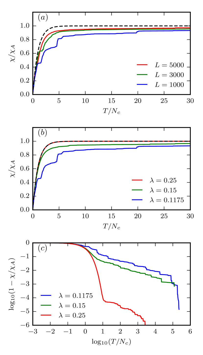
Figure 5: Filling of cells as a function of the number of orbit iterations (a) for different grid sizes at $\lambda=0.1175$ and (b) for different values of $\lambda$ at grid size $L=1000$. The proportion of filled cells is normalized to the asymptotic value at $T=10^{11}$ iterations and the iterations are given in terms of the number of chaotic cells $N_{C}=\chi_{A}L^{2}$. The black dashed curve shows the prediction of the random model Eq. 5. (c) The difference of the proportion of filled cells to the asymptotic value in the log-log scale for the same values of $\lambda$ and grid size as in panel (b) (the order of the curves from top to bottom is indicated by the legend in each panel).

It is useful to consider not only whether a cell gets filled but also its occupancy, meaning the number of times it is visited. A plot of the cell occupancy for the $\lambda=0.15$ billiard after $10^{11}$orbit iterations is presented in Fig. 6. Because of symmetry we show only one quadrant of the phase space. Inside the chaotic sea the cell occupancy is quite uniform with the majority of cells having an occupancy close to $M\approx\mu=\frac{T}{\chi_{C}L^{2}}$, within the expected standard deviation given by the random model $\sigma=\sqrt{\mu}$. Notable differences occur in the occupancy of the cells on the borders of the KAM islands and near the Lazutkin tori. In these one can see a difference of more than $5\sigma$ from the average occupancy. Unusually large occupancy numbers indicate areas with sticky objects. Conversely, areas with unusually small occupancy indicate that transport into these areas is limited by some barrier like for instance a cantorus. Once the orbit penetrates the area bordered by a cantorus it may be traped there for some time.

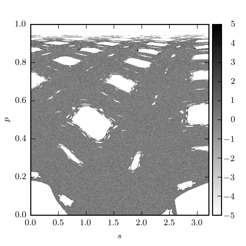
Figure 6: Cell occupancy in one quadrant of the phase space for $\lambda=0.15$, $L=3000$ and $T=10^{11}$. The grayness indicates the occupancy as the difference to the average $\mu=\frac{T}{\chi_{C}L^{2}}$. The scale is given in units of the standard deviation $\sigma=\sqrt{\mu}$.

The occupancy distributions of the cells after $10^{11}$ orbit iterations are presented in Fig. 7. Panels (a), (b), (c) show the distributions for $L=1000$ and $\lambda=0.15$, $\lambda=0.25$, $\lambda=0.5$, respectively. The histograms are fitted with the Poissonian distribution Eq. (8) which closely coincides with the histograms in these three cases. On the other hand the histogram for $\lambda=0.1175$ and $L=1000$ in panel (d) is markedly different from the Poissonian distribution and exhibits some asymmetry with regard to the mean value. The asymmetry is greatly diminished if the cell size is decreased and the histograms are again close to Poissonian as shown in panels (e) and (f). We stress that the only difference in panels (d), (e) and (f) is the grid of cells, the orbit is exactly the same. The occupancy distributions also have a peak of height $1-\chi_{A}$ at $M=0$ because of the empty cells. The exception is $\lambda=0.5$ where, due to ergodicity all cells are filled.

The fact that the cell occupancy distributions are close to Poissonian implies that the cell visits are in the long term uncorrelated, provided the cells are small enough. Even though the chaotic orbit may spend a significant number of iterations trapped in the vicinity of sticky objects this is averaged out in the long term. This suggests that the time between successive trappings is longer than the time of the trapping episodes. The more complex the phase space the longer it takes (in terms of the number of orbit iterations) to reach the Poissonian limit. If the phase space is simple like for instance in the $\lambda=0.25$ and $\lambda=0.5$ the limiting occupancy distribution is reached before $10^{10}$ orbit iterations for $L=1000$. In contrast, for the most complex case $\lambda=0.1175$ the distribution is far from Poissonian even after $10^{11}$ orbit iterations. Decreasing the cell size (increasing $L$) generally improves the rate of convergence. The average occupancy of the cells may be used to estimate the measure of the chaotic component, since the relation $\mu=\frac{T}{\chi_{C}L^{2}}$ should hold. The naive estimate from the number of filled cells $\chi_{A}$ and from the average of the occupancy distribution $\chi_{C}$ are slightly different, as will be shown in more detail in Sec. VI.

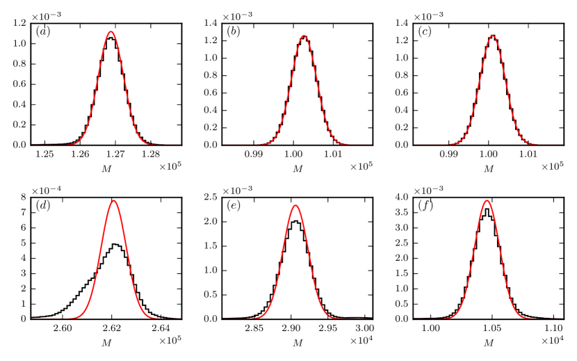
Figure 7: Histograms of the occupancy distributions. Top row $L=1000$ and (a) $\lambda=0.15$ , (b) $\lambda=0.25$ , (c) $\lambda=0.5$. Bottom row $\lambda=0.1175$ and (d) $L=1000$, (e) $L=3000$, (f) $L=5000$. The Poissonian distribution Eq. (8), expected from the random model, is fitted to the histograms and shown with the red curve. The number of orbit iterations is $T=10^{11}$.

V Cell recurrence times

Further information about the structure of the phase space may be gained from the (discrete) cell recurrence times. Recurrence times statistics are one of the standard ways of quantifying stickiness (Altmann et al., 2004, 2005, 2006; Abud and de Carvalho, 2013). We define the cell recurrence time $\tau$ for each individual cell as the number of iterations an orbit needs to return to the same cell for the first time. If the motion on the chaotic component is ergodic, it follows from the Kac lemma (Kac, 1959), that the average first return time $\mu_{\tau}$ to a cell is equal to the inverse of the normalized measure of the cell, which is equal the number of cells in the chaotic component $\mu_{\tau}=\chi_{C}L^{2}=N_{C}$. Additionally, if the cell visits are completely uncorrelated (random model) the probability that a cell is visited after any number of iterations is equal. The probability distribution of cell return times is thus exponential

$$P\left(\tau\right)=\frac{1}{\mu_{\tau}}\exp\left(-\frac{\tau}{\mu_{\tau}}\right),$$ (9)

The variance of this distribution is $\sigma_{\tau}^{2}=\mu_{\tau}^{2}$.

Now we will take into account that the samples in our numerical experiments are finite. We define the normal distribution as

$$\mathcal{N}\left(x,\mu,\sigma\right)=\frac{1}{\sqrt{2\pi\sigma^{2}}}\exp\left(-\frac{\left(x-\mu\right)^{2}}{2\sigma^{2}}\right),$$ (10)

where $\mu$ and $\sigma$ are the mean and standard deviation of the normal distribution. Let $x$ be some observable distributed according to the probability distribution $P\left(x\right)$ with a finite mean $\mu_{x}$ and variance $\sigma_{x}^{2}$. Let $\overline{x}$ be the mean of $x$ as calculated from a sample of $N$ values. From the central limit theorem (Feller, 1968) it follows that $\overline{x}$ is distributed according to the normal distribution $\mathcal{N}\left(\overline{x},\mu_{x},\frac{\sigma_{x}}{\sqrt{N}}\right)$. If the cell visits are uncorrelated, the distribution of the average cell return times $\overline{\tau}$ is normal

$$P\left(\overline{\tau}\right)=\mathcal{N}\left(\overline{\tau},N_{C},\frac{N_{C}^{\frac{3}{2}}}{\sqrt{T}}\right),$$ (11)

where the mean and standard deviation are determined using the exponential distribution Eq. (9) and the estimate that each cell is visited $N=\frac{T}{N_{C}}$ times for the sample size.

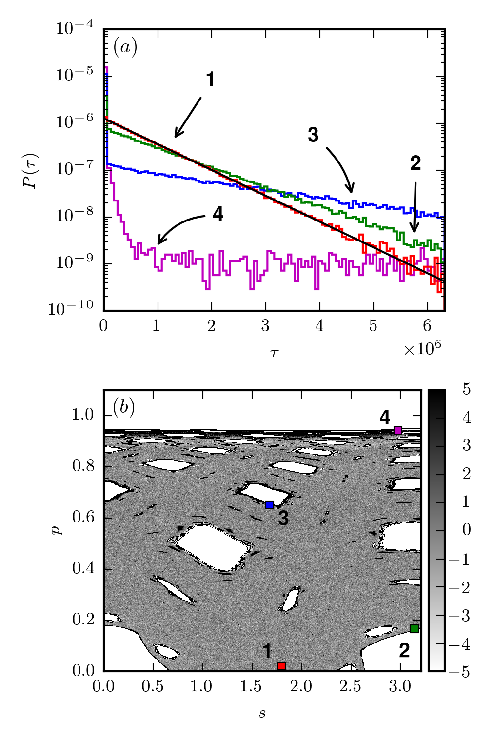
Figure 8: Cell return times in the $\lambda=0.15$ billiard, with $L=1000$ and $T=10^{11}$. (a) Histograms of cell return times for four different cells at the following coordinates $(s,p)=(1.80,\,0.022)$ red 1, (3.14, 0.17) green 2, (1.67, 0.65) blue 3, (2.97, 0.94) magenta 4. The exponential distribution from the random model Eq. 9 is plotted with the black line. (b) The average return times $\overline{\tau}$ in one quadrant of the phase space. The shade indicates the difference from the average $\mu_{\tau}=N_{C}$ in units of the expected standard deviation $\sigma_{\overline{\tau}}=N_{C}^{3/2}/\sqrt{T}$. The colored and numbered boxes show the positions of the cells from panel (a) (The size of the boxes does not correspond to the size of the cells).

The histograms of the cell recurrence times in four different cells in the $\lambda=0.15$ billiard are presented in Fig. 8 (a). The first cell (red) is located in the middle of the chaotic sea far from any KAM islands. The distribution of return times closely coincides with the exponential distribution Eq. (9). All cells sufficiently deep inside chaotic sea exhibit this kind of exponential distribution of cell return times. This means that the majority of cells experiences completely uncorrelated orbit visits. The second cell (green) is located on the border of one of the largest KAM islands. The distribution is still close to exponential with a slightly different exponent but has a small peak at short return times. The change in the exponential is a consequence of the increased probability of short recurrence times due to memory effects i. e. stickiness (see Ref. [Altmann et al., 2004]). We would like to emphasize that the recurrences to the cell are generated by a single chaotic orbit. Even if the cell partly intersects a regular region the orbit only visits the chaotic part of the cell. The distributions of return times from a regular component are expected to exhibit power law tails (N Buric and Vaienti, 2003; Hu et al., 2004). The third cell (blue) is located on the border of the smaller KAM island. The cell return time distribution is qualitatively similar to that in the second cell but with a much higher peak at short times and the long time tail is stronger. The fourth cell (magenta) is located near the Lazutkin torus. The cell return time distribution is even more severely peaked at the short return times, while the tail is very long but still exponential. The orbit visits this cell either in quick succession or after very long periods of time resulting in a distribution with a large variance. The variance (or standard deviation) of the return times in a cell may thus be a good measure of the stickiness of a cell.

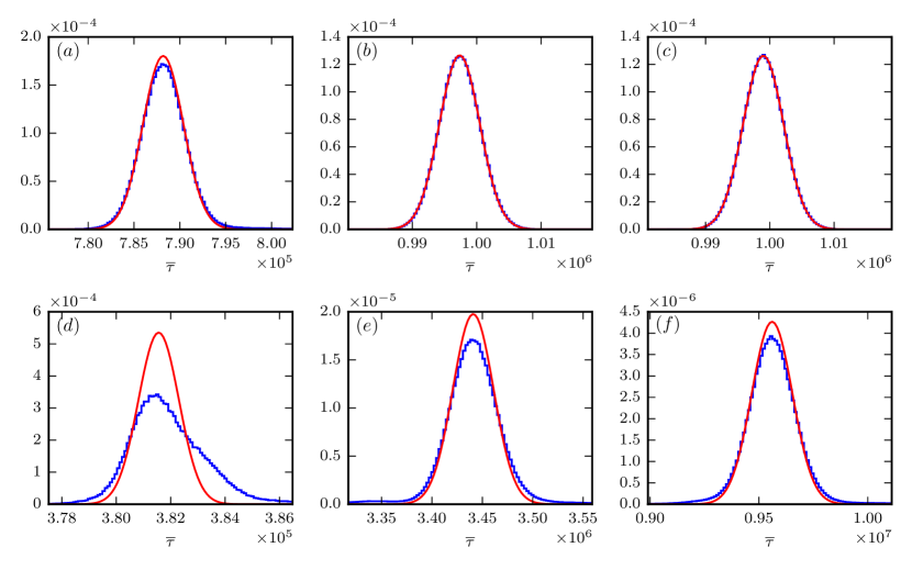
Figure 9: Histograms of the average cell return times. Top row $L=1000$ and (a) $\lambda=0.15$ , (b) $\lambda=0.25$ , (c) $\lambda=0.5$. Bottom row $\lambda=0.1175$ and (d) $L=1000$, (e) $L=3000$, (f) $L=5000$. The normal distribution Eq. (11) is plotted with the red curve. The number of orbit iterations is $T=10^{11}$.

To gain a global understanding of the cell return times, the average return times in one quadrant of the phase space are shown in panel (b) of the same figure together with the positions of the aforementioned cells. The average cell return time is mostly uniform in the chaotic sea. Differences of more than five standard deviations can be seen mostly around the KAM islands and near the Lazutkin torus. The histograms of the average return times for different sets of parameters are shown in Fig. 9. They are compared with the random model prediction Eq. (11). We see that the histograms agree well with the normal distribution for $\lambda=0.15$, $\lambda=0.25$ and $\lambda=0.5$ at grid size $L=1000$, while for $\lambda=0.1175$ there is a deviation similar to the one found in the occupancy distribution. This deviation diminishes when the cell size is decreased. The average cell return times hold essentially the same information about the dynamics as the cell occupancy numbers.

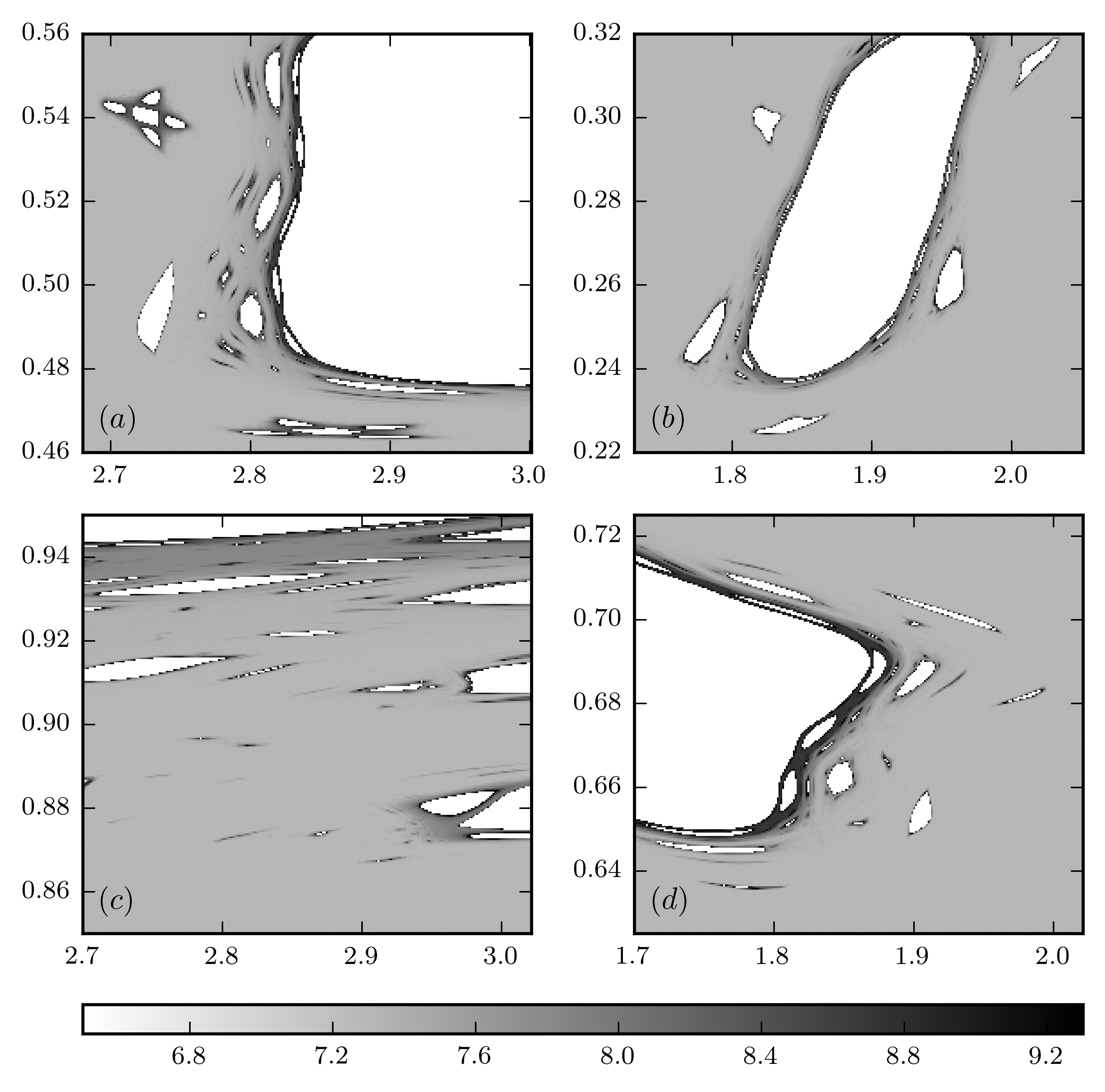
Figure 10: The standard deviation of cell return times in selected areas of phase space for the $\lambda=0.15$ billiard, with $L=5000$ and $T=10^{11}$. The greyness scale is logarithmic with base 10.

A global quantitative assessment of the stickiness of the various structures present in the phase space can be made from the standard deviations (or variances) of the cell return times. Fig. 10 shows logarithmic color plots of the cell return time standard deviations in the $\lambda=0.15$ billiard. Panel (a) shows the phase space area near the border of one of the KAM islands formed around the stable periodic orbit with period three, panel (b) near a KAM island of the star shaped period five orbit, panel (c) near the Lazutkin torus and (d) near a KAM island of the pentagonal shaped period five orbit. The sizes of the areas depicted are the same for each panel. In the chaotic sea, the cell return time standard deviation is uniform, while the structures in the phase space exhibit various degrees of stickiness. For most of the KAM islands the standard deviation of the cell return times increases roughly exponentially (linearly in the logarithmic scale of the plot) in the vicinity of the border. An abrupt rather than gradual increase in the standard deviation implies a cantorus acting as a barrier to the orbit. This can be clearly seen in the upper part of panel (c). Upon closer inspection one can see that the darkest areas around the largest KAM islands in panels (a) and (d) also have an abrupt border followed by an exponential decay. High resolution phase portraits of the cell return time standard deviations in the largest chaotic component for various $\lambda$ are made available in the supplemental materials (SM, ).

VI The measure of the chaotic component

The statistical properties of the filling of the phase space cells discussed in the previous sections may be used to determine the measure of the chaotic components in several ways:

1. The simplest estimate for the measure is the proportion of filled cells in the long time limit $\chi_{A}$. The number of cells visited after a set number of orbit iterations is counted and divided by the number of all cells.

2. The measure can be obtained from the cell occupancy distributions. Assuming the motion of the orbit on the chaotic component is ergodic in the long term the visitation probability is distributed according to the Poissonian distribution Eq. (8), with $\mu=\frac{T}{\chi_{C}L^{2}}$. The histogram of cell occupancies is fitted with the Poissonian and the measure $\chi_{C}$ extracted.

3. The measure can be obtained from the cell return times. If the motion of the orbit is uncorrelated the probability that the mean first return time to a cell $\overline{\tau}$ is given by the normal distribution Eq. (11), centered at $\mu_{\tau}=\chi_{C}L^{2}=N_{C}$ and with a standard deviation of $\sigma_{\overline{\tau}}=N_{C}^{3/2}/\sqrt{T}$. The normal distribution is fitted to the histogram of mean return times and $\chi_{C}$ is extracted.

The results for the measure of the largest chaotic component in the $\lambda=0.15$, determined by the three different methods, are compared in Fig. 11. The two numerical parameters in the calculation are the number of orbit iterations $T$ and the grid size $L$. It is advisable that the number of iterations is several decadic orders of magnitude larger than the number of cells. Of the three methods of determining the measure of the chaotic component method 1 has the strongest dependence on $L$. As already mentioned some cells may be only partially filled by the chaotic component whereas using method 1 the whole area of these cells is attributed to the chaotic component. Because the border of the chaotic component is fractal this may lead to a significant overestimation of its measure. Increasing $L$ and thus improving the resolution in the phase space can significantly decrease this overestimation. Since each cell is counted as soon as the orbit visits it, the estimate for the measure of the chaotic component using method 1 is an increasing function of $T$. This method may serve as an upper estimate provided the number of orbit iterations is large enough for the orbit to visit all the cells at least partially containing the chaotic component.

The benefit of method 2 is that it takes into account not only if the cell was visited but also the number of cell visits. Cells that are seldom visited have a high probability of being positioned near the border and only containing a small part of the chaotic component. The cells in the chaotic sea form the most significant contribution. This method assumes that in the long term the motion of the orbit on the chaotic component is ergodic and the episodes of trapping average out. It is also important that orbit permeates all the areas of the chaotic component bordered by strong barriers like cantori. Because of this the number of iterations needed to achieve convergence may be very large. In Fig. 11 we see that the estimates for the measure at $T=10^{10}$ and $T=10^{11}$ differ significantly. The shape of the histogram also serves as a good indication if the grid size is sufficient. In the case of $\lambda=0.15$ the shape is close to Poissonian already at $L=1000$ (see Fig. 7) and increasing it to $L=3000$ has only a small effect and the results for $L=5000$ overlap. The results of using method 3 i.e. the cell return time histograms practically overlap with those of method 2. This is to be expected as the mean return time to a cell is the number of orbit iterations divided by the number of visits.

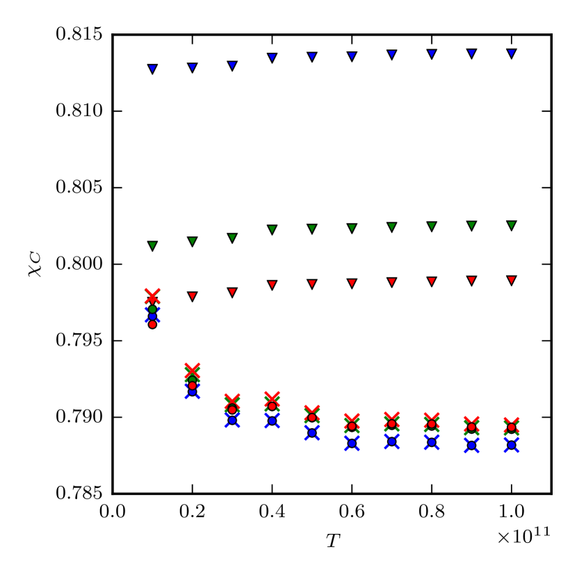
Figure 11: The measure of the largest chaotic component in the $\lambda=0.15$ as determined by three different methods as a function of the number of orbit iterations $T$ and grid size $L$. The colors denote the grid size $L=1000$ blue, $L=3000$ green, $L=5000$ red. The markers denote the method used. Method 1 (see list in main text) is represented by triangles, method 2 by circles and method 3 by exes. The orbit was exactly the same in all cases.

Our main motivation for developing methods for determining the measure of the chaotic component stems from the study of energy level statistics in the context of quantum chaos in generic autonomous Hamiltonian systems like for instance a quantum billiard of the same shape (Batistić and Robnik, 2010, 2013a, 2013b). In the strict semiclassical limit it is possible to separate chaotic eigenstates from regular ones (see Refs. (Percival, 1973; Berry, 1977; Voros, 1979; Shnirelman, 1979; Berry and Robnik, 1984; Robnik, 1998; Veble et al., 1999; Batistić and Robnik, 2010, 2013a, 2013b) and references therein). In the mixed-type regime, following the so-called principle of uniform semiclassical condensation (of Wigner functions of the eigenstates), Berry-Robnik (or Berry-Robnik-Brody in the case of dynamical localization) statistics is observed. The full spectrum is a linear superposition of the spectrum of the chaotic eigenstates and the spectrum of the regular eigenstates. The relative contributions of the separated spectra in the Berry-Robnik(-Brody) statistics are given by the fractional Liouville measure of the chaotic component $\rho_{C}$ on the classical energy surface (i.e. the energy surface of the equivalent classical system) and the measure of the regular components $\rho_{R}=1-\rho_{C}$. Thus far we were involved with determining the (fractional) measure of the chaotic component $\chi_{C}$ on the Poincaré surface of section (SOS). This is related to the fractional Liouville measure on the energy surface via the following relation (Meyer, 1986)

$$\rho_{C}=\frac{\chi_{C}}{\chi_{C}+\left(1-\chi_{C}\right)\xi},$$ (12)

where $\xi=\frac{\left\langle t\right\rangle_{R}}{\left\langle t\right\rangle_{C}}$ is the ratio between the average return time to the SOS on the regular components $\left\langle t\right\rangle_{R}$ and the average of the same quantity on the chaotic component $\left\langle t\right\rangle_{C}$. For the equivalent formula for $\rho_{R}=1-\rho_{C}$ we only need to exchange the indices $R\leftrightarrow C$ and invert the ratio $\xi\rightarrow 1/\xi$ in Eq. (12). In billiards the SOS is the billiard boundary and the ratio $\xi$ is independent of the speed of the particle. The SOS return time is proportional to the length of a link of a trajectory. The ratio $\xi$ can thus be determined by averaging the length of a link over a number of collisions and calculating the averages with regard to the initial conditions. The measures of the chaotic component on the SOS as well as the associated Liouville measures on the energy surface are given in table 2 for various $\lambda$.

$\lambda$	$\chi_{C}$	$\chi_{A}$	$\rho_{C}$
0.1175	0.382	0.397	0.452
0.125	0.548	0.569	0.613
0.13	0.600	0.611	0.662
0.135	0.662	0.674	0.718
0.14	0.707	0.717	0.755
0.15	0.789	0.798	0.824
0.16	0.855	0.862	0.876
0.18	0.946	0.950	0.952
0.2	0.976	0.977	0.975
0.23	0.996	0.997	0.996
0.25	0.999	0.999	0.999
0.5	1	1	1

Table 2: Table of values for the fractional measure of the largest chaotic component. $\chi_{C}$ is the value for the measure on the SOS, obtained from fitting the occupancy distribution, $\chi_{A}$ is the proportion of filled cells at $T=10^{11}$ and $\rho_{C}$ is the measure on the energy surface calculated from $\chi_{C}$, using Eq.(12). The cell grid size was $L=5000$.

VII The correlation functions and momentum diffusion

The phenomenon of stickiness has been shown to lead to non-exponential or power law decay of correlations. As a means of studying the decay of correlations in our family of billiards we chose the momentum autocorrelation function defined as

$$C_{pp}\left(n\right)=\lim_{T\rightarrow\infty}\frac{1}{T}\sum_{t=0}^{T}p\left(x_{t}\right)p\left(x_{t+n}\right),$$ (13)

where $p\left(x_{i}\right)$ denotes the momentum of the particle after the $i$-th mapping of the orbit $x_{i}$ with initial condition $x_{0}$. It is convenient to normalize the autocorrelation function by its initial value $C\left(n\right)=\frac{C_{pp}\left(n\right)}{C_{pp}\left(0\right)}$. The decay of the normalized momentum autocorrelation functions is depicted in Fig. 12. Panel (a) shows $C\left(n\right)$ for 24 orbits in the $\lambda=0.15$ billiard. The initial conditions were selected at random inside the largest chaotic component. Some orbits start deep inside the chaotic sea while others start near the various phase space structures like the KAM islands or near the Lazutkin torus. We see that the decay of correlations differs significantly from orbit to orbit. The average over all 24 initial conditions is shown with the black line. The tail of this average obeys a power law (linear in the log-log scale) $C\left(n\right)\sim n^{-\alpha}$ with $\alpha\approx 0.68$. Panel (b) shows $C\left(n\right)$ for 24 orbits in the $\lambda=0.5$ billiard i.e. the ergodic case. The decay of correlations here is very rapid with $C\left(n\right)$ reaching the 0.1 value in about ten orbit iterations. The different initial conditions produce practically the same results with the small differences being attributed to numerical fluctuations. The tail of the average also decays as a power with $\alpha=2$. This may be considered counter intuitive as the system is ergodic and, in contrast to some other prominent billiards like the stadium, has no families of marginally unstable periodic orbits, that have been shown to produce such effects (Vivaldi et al., 1983). But it has also been shown that in the stadium billiard the power law tails of the correlations are caused also by the orbits only glancing the boundary and spending a significant number of iterations in integrable motion on one of the stadium semicircles. These have been specifically associated with a power law decay with $\alpha=2$. While there is no complete analogy for this type of integrable motion in the $\lambda=0.5$ billiard an orbit with a very large angle of incidence may still spend a significant number of bounces glancing the boundary with the angle changing only slightly and thus sticking to the edge of the phase space until the inevitable flyaway, when it reaches the cusp singularity at $z=-1$. It is important to note that if we were to study the billiard in continuous time i.e. the billiard flow instead of the billiard map, the quick succession of the bounces would eliminate this type of stickiness.

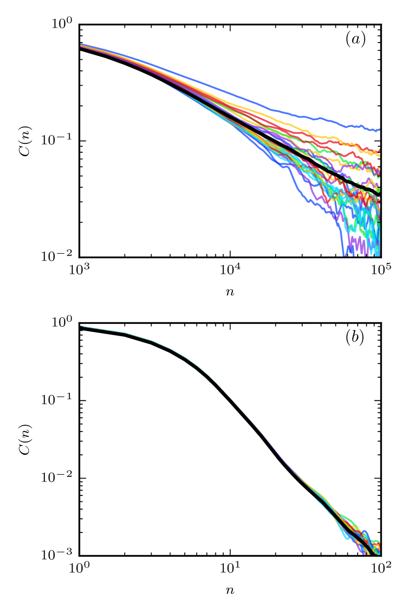
Figure 12: The normalized momentum autocorrelation functions in the $\lambda=0.15$ billiard (a) and the ergodic $\lambda=0.5$ billiard (b). The colored lines depict the autocorrelation functions for 24 initial conditions selected randomly in the largest chaotic component. The black line is the average over all 24 initial conditions. The orbits were iterated $T=10^{8}$ times for the calculation of the autocorrelation functions.

Lastly we turn our attention to the diffusion in momentum space. In a previous paper (Lozej and Robnik, 2018) we explored the momentum diffusion of ensembles of particles in the stadium billiard and found that the diffusion was well described by an inhomogeneous diffusion model with a diffusion constant that is a quadratic function of the momentum. We have shown that the variance of the momenta of an ensemble of particles distributed along the billiard boundary and with initial momentum $p_{0}$ approaches its asymptotic value exponentially. A similar numerical experiment may be performed for the family of $\lambda$ billiards. Firstly, we note that momentum diffusion may only be present on the chaotic component and not on the regular ones. We thus selected an ensemble of $10^{5}$ particles with initial conditions $p=0$ (the initial velocity of the particles is perpendicular to the boundary) and $s$ in the chaotic sea. The particles then bounce inside the billiard and the variance of their momenta $\mathrm{Var}(p)$ is recorded with each bounce. Eventually, the particles should distribute themselves uniformly across the chaotic component and the asymptotic value of the variance $A$ should be reached. In contrast to the stadium billiard the value of $A$ can not be easily obtained analytically due to the complex structure of the phase space (the exception is $\lambda=0.5$). The value of $A$ was determined numerically from the phase portraits at $L=5000$ and should be accurate within one percent. In Fig. 13 the results for $\lambda=0.135,$ 0.15 and 0.16, with $p_{0}=0$ are shown. Panel (a) shows the variance of the momentum as a function of the number of bounces. The results for all three $\lambda$ are qualitatively similar. An initial rapid increase of the variance is followed by a slow approach to the asymptotic value. This is quite different to the case of the stadium where the variance was globally well described by an exponential decay to the asymptotic value. This slow decay to the asymptotic value is probably a consequence of the labyrinthine complexity of the phase space and the trapping of orbits by sticky objects. The approach to the asymptotic value in the log-log scale is portrayed on panel (b). The approach to the asymptotic value seems to be neither exponential nor a power law.

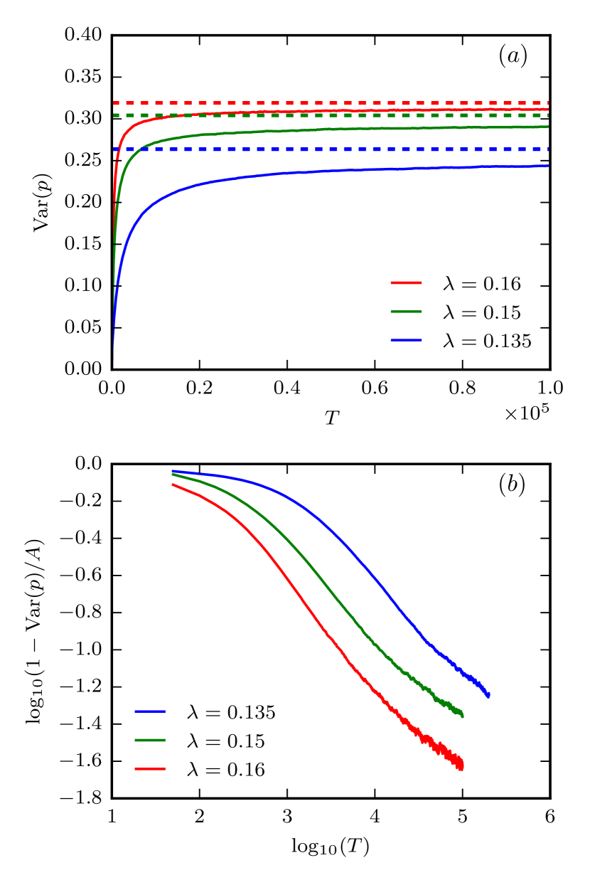
Figure 13: Momentum diffusion in the $\lambda=0.135$, $\lambda=0.15$ and $\lambda=0.16$ billiards. (a) The variance of the momenta of an ensemble of $10^{5}$ particles as a function of the number of bounces. The particles all have an initial momentum of $p=0$ and $s$ from the chaotic component. The expected asymptotic value of the variance, calculated from the phase portrait, is plotted with a dashed line. (b) The approach to the asymptotic value in the log-log scale (the order of the curves from top to bottom is indicated by the legend in each panel).

VIII Discussion and conclusions

We have shown that in generic (mixed-type) Hamiltonian systems the complexity of the phase space and the intermittency of the chaotic dynamics pose a serious challenge when determining the size and structure of the chaotic component. When the phase space is divided into cells the cell visitations by a chaotic orbit are not completely uncorrelated even for very small cells. The orbit may be trapped by sticky objects or cantori for significant periods of time. The standard deviation of the cell recurrence time may be a good observable for quantifying stickiness on the global level. The standard deviation of the cell recurrence times decays roughly exponentially with the distance to the sticky object. The vast majority of cells in the chaotic component experience completely uncorrelated visits, as evidenced also by the recurrence time distributions. In the long run the intermittent behavior of the chaotic orbit averages out and the cell visitation statistics concur with the random model. From there one can extract the measure of the chaotic component, either from the distribution of the cell visitation numbers or the average recurrence times, to a high degree of accuracy.

This method is an improvement over simply counting the number of chaotic cells and is less dependent on cell size. However, we must stress that the number of orbit iterations needed for the desired accuracy may still be very large, in our case $10^{11}$. A nice feature of the method is also that the only prior knowledge of the system we need is one initial condition in the chaotic component we wish to measure. The method should be applicable to a wide range of dynamical systems and is a priori not limited to two dimensions, although the scaling of the cell volume might make its use prohibitive in higher dimensions. One of the ways in which this problem might be addressed is by computing the cell visits of several chaotic orbits in parallel and combining the results.

As has been observed in previous examples, stickiness leads to power law decay of correlations also in our family of billiards. The momentum diffusion also behaves differently than in the stadium billiard where the approach of the variance of the momenta to the asymptotic value is exponential. The classical transport time (or diffusion time) is an important parameter in the study of dynamical localization in quantum chaos. In the stadium it was possible to define the classical transport time in a clear way, by using this exponential law. It is not possible to define the classical transport time for the family of billiards used in this paper in the same way and this remains an open question. Our current working definition involves measuring the time it takes for the variance to reach an arbitrary proportion of the asymptotic value and further work is in progress.

References

- Bunimovich and Vela-Arevalo (2012) L. A. Bunimovich and L. V. Vela-Arevalo, Chaos: An Interdisciplinary Journal of Nonlinear Science 22, 026103 (2012).
- Contopoulus and Harsoula (2010) G. Contopoulus and M. Harsoula, International Journal of Bifurcation and Chaos 20, 2005 (2010).
- MacKay et al. (1984) R. S. MacKay, J. D. Meiss, and I. C. Percival, Phys. Rev. Lett. 52, 697 (1984).
- Mackay et al. (1984) R. Mackay, J. Meiss, and I. Percival, Physica D: Nonlinear Phenomena 13, 55 (1984).
- Chirikov and Shepelyansky (1984) B. Chirikov and D. Shepelyansky, Physica D: Nonlinear Phenomena 13, 395 (1984).
- Chirikov and Shepelyansky (1999) B. V. Chirikov and D. L. Shepelyansky, Phys. Rev. Lett. 82, 528 (1999).
- Vivaldi et al. (1983) F. Vivaldi, G. Casati, and I. Guarneri, Phys. Rev. Lett. 51, 727 (1983).
- Zaslavsky (2002) G. Zaslavsky, Physics Reports 371, 461 (2002).
- Cristadoro and Ketzmerick (2008) G. Cristadoro and R. Ketzmerick, Phys. Rev. Lett. 100, 184101 (2008).
- Abud and de Carvalho (2013) C. V. Abud and R. E. de Carvalho, Phys. Rev. E 88, 042922 (2013).
- Young (1998) L.-S. Young, Annals of Mathematics 147, 585 (1998).
- Young (1999) L.-S. Young, Israel Journal of Mathematics 110, 153 (1999).
- Hirata et al. (1999) M. Hirata, B. Saussol, and S. Vaienti, Communications in Mathematical Physics 206, 33 (1999).
- Bunimovich (1979) L. A. Bunimovich, Comm. Math. Phys. 65, 295 (1979).
- Markarian (2004) R. Markarian, Ergodic Theory and Dynamical Systems 24, 177 (2004).
- Percival (1973) I. C. Percival, Journal of Physics B: Atomic and Molecular Physics 6, L229 (1973).
- Berry (1977) M. V. Berry, Journal of Physics A: Mathematical and General 10, 2083 (1977).
- Voros (1979) A. Voros, in Lecture notes in Physics, Vol. 93 (Springer Berlin, 1979) pp. 326–333.
- Shnirelman (1979) A. L. Shnirelman, Uspekhi Matem. Nauk 29, 181 (1979).
- Berry and Robnik (1984) M. V. Berry and M. Robnik, Journal of Physics A: Mathematical and General 17, 2413 (1984).
- Robnik (1998) M. Robnik, Nonlinear Phenomena in Complex Systems (Minsk) 1, 1 (1998).
- Veble et al. (1999) G. Veble, M. Robnik, and J. Liu, Journal of Physics A: Mathematical and General 32, 6423 (1999).
- Batistić and Robnik (2010) B. Batistić and M. Robnik, J. Phys. A: Math. Theor. 43, 215101 (2010).
- Batistić and Robnik (2013a) B. Batistić and M. Robnik, J. Phys. A: Math. Theor. 46, 315102 (2013a).
- Batistić and Robnik (2013b) B. Batistić and M. Robnik, Phys. Rev. E 88, 052913 (2013b).
- Batistić et al. (2018) B. Batistić, Č. Lozej, and M. Robnik, in preparation (2018).
- Robnik (1983) M. Robnik, J. Phys. A: Math. Gen. 16, 3971 (1983).
- Markarian (1993) R. Markarian, Nonlinearity 6, 819 (1993).
- Berry (1981) M. V. Berry, Eur. J. Phys. 2, 91 (1981).
- Lazutkin (1973) V. F. Lazutkin, Mathematics of the USSR-Izvestiya 7, 185 (1973).
- Mather (1982) J. N. Mather, Ergodic Theory and Dynamical Systems 2, 397 (1982).
- Benettin et al. (1976) G. Benettin, L. Galgani, and J.-M. Strelcyn, Phys. Rev. A 14, 2338 (1976).
- Dobnikar (1996) J. Dobnikar, “Diploma thesis: Spectral statistics in the transition between integrability and chaos with broken antiunitary symetry, CAMTP and University of Ljubljana,” (1996).
- Ott (2002) E. Ott, Chaos in Dynamical Systems, 2nd ed. (Cambridge University Press, 2002).
- Lozej and Robnik (2018) Č. Lozej and M. Robnik, Phys. Rev. E 97, 012206 (2018).
- Robnik et al. (1997) M. Robnik, J. Dobnikar, A. Rapisarda, T. Prosen, and M. Petkovšek, J. Phys. A: Math. Gen. 30, L803 (1997).
- Feller (1968) W. Feller, An Introduction to Probability Theory and Its Applications, 3rd ed. (Wiley, 1968).
- Altmann et al. (2004) E. G. Altmann, E. C. da Silva, and I. L. Caldas, Chaos: An Interdisciplinary Journal of Nonlinear Science 14, 975 (2004).
- Altmann et al. (2005) E. G. Altmann, A. E. Motter, and H. Kantz, Chaos: An Interdisciplinary Journal of Nonlinear Science 15, 033105 (2005).
- Altmann et al. (2006) E. G. Altmann, A. E. Motter, and H. Kantz, Phys. Rev. E 73, 026207 (2006).
- Kac (1959) M. Kac, Probability and Related Topics in Physical Sciences (Interscience Publishers, 1959).
- N Buric and Vaienti (2003) G. T. N Buric, A Rampioni and S. Vaienti, Journal of Physics A: Mathematical and General 36, 7223 (2003).
- Hu et al. (2004) H. Hu, A. Rampioni, L. Rossi, G. Turchetti, and S. Vaienti, Chaos: An Interdisciplinary Journal of Nonlinear Science 14, 160 (2004).
- (44) See Supplemental Material at [URL will be inserted by publisher] for high resolution phase portraits of the cell recurrence time standard deviations.
- Meyer (1986) H. Meyer, The Journal of Chemical Physics 84, 3147 (1986).
- (46) Available at https://github.com/benokit/time-dep-billiards.