Applications of physics-informed scientific machine learning in subsurface science: A survey

Bureau of Economic Geology, Jackson School of Geosciences, The University of Texas at Austin, Austin, TX Geomechanics Department, Sandia National Laboratories, Albuquerque, NM Leidos, Pittsburgh, PA School of Earth Resources, China University of Geosciences, Wuhan, China

A. Y. Sunalex.sun@beg.utexas.edu

Geosystems are geological formations altered by humans activities such as fossil energy exploration, waste disposal, geologic carbon sequestration, and renewable energy generation. Geosystems also represent a critical link in the global water-energy nexus, providing both the source and buffering mechanisms for enabling societal adaptation to climate variability and change. The responsible use and exploration of geosystems are thus critical to the geosystem governance, which in turn depends on the efficient monitoring, risk assessment, and decision support tools for practical implementation. Large-scale, physics-based models have long been developed and used for geosystem management by incorporating geological domain knowledge such as stratigraphy, governing equations of flow and mass transport in porous media, geological and initial/boundary constraints, and field observations. Spatial heterogeneities and the multiscale nature of geological formations, however, pose significant challenges to the conventional numerical models, especially when used in a simulation-based optimization framework for decision support. Fast advances in machine learning (ML) algorithms and novel sensing technologies in recent years have presented new opportunities for the subsurface research community to improve the efficacy and transparency of geosystem governance. Although recent studies have shown the great promise of scientific ML (SciML) models, questions remain on how to best leverage ML in the management of geosystems, which are typified by multiscality, high-dimensionality, and data resolution inhomogeneity. This survey will provide a systematic review of the recent development and applications of domain-aware SciML in geosystem researches, with an emphasis on how the accuracy, interpretability, scalability, defensibility, and generalization skill of ML approaches can be improved to better serve the geoscientific community.

1 Introduction

Compartments of the subsurface domain (e.g., vadose zone, aquifer, and oil and gas reservoirs) have provided essential services throughout the human history. The increased exploration and utilization of the subsurface in recent decades, exemplified by the shale gas revolution, geological carbon sequestration, and enhanced geothermal energy recovery, have put the concerns over geosystem integrity and sustainability under unprecedented public scrutiny (Elsworth et al., 2016; yeo2020causal). In this chapter, geosystems are defined broadly as the parts of lithosphere that are modified directly or indirectly by human activities, including mining, waste disposal, groundwater pumping and energy production (National Research Council, 2013). Anthropogenic-induced changes may be irreversible and have cascading social and environmental impacts (e.g., overpumping of aquifers may cause groundwater depletion, leading to land subsidence and water quality deterioration, and increasing the cost of food production). Thus, the sustainable management of geosystems calls for integrated site characterization, risk assessment, and monitoring data analytics that can lead to better understanding while promoting inclusive and equitable policy making. Importantly, system operators need to be able to explore and incorporate past experience and knowledge, gained either from the same site or other similar sites, to quickly identify optimal management actions, detect abnormal system signals, and to prevent catastrophic events (e.g., induced seismicity and leakage) from happening.

Fast advances in machine learning (ML) technologies have revolutionized predictive and prescriptive analytics in recent years. Significant interests exist in harnessing this new generation of ML tools for Earth system studies (Reichstein et al., 2019; Sun and Scanlon, 2019; Bergen et al., 2019). Unlike many other sectors, however, subsurface formations are often poorly characterized and scarcely monitored, thus relying extensively upon geological and geofluid modeling to generate spatially and temporally continuous “images” of the subsurface. A conventional workflow may consist of (a) geologic modeling, which seeks to provide a 3D representation of the geosystem under study by fusing qualitative interpretation of the geological structure, stratigraphy, and sedimentological facies, as well as quantitative data on geologic properties; and (b) fluid and geomechanical modeling, which describes the fluid flow, mass transport, and formation deformations through physics-based governing equations and the accompanying initial/boundary/forcing conditions. Once established, the workflow is used to generate 3D “images” of the subsurface processes for inference and/or prediction (Figure 1).

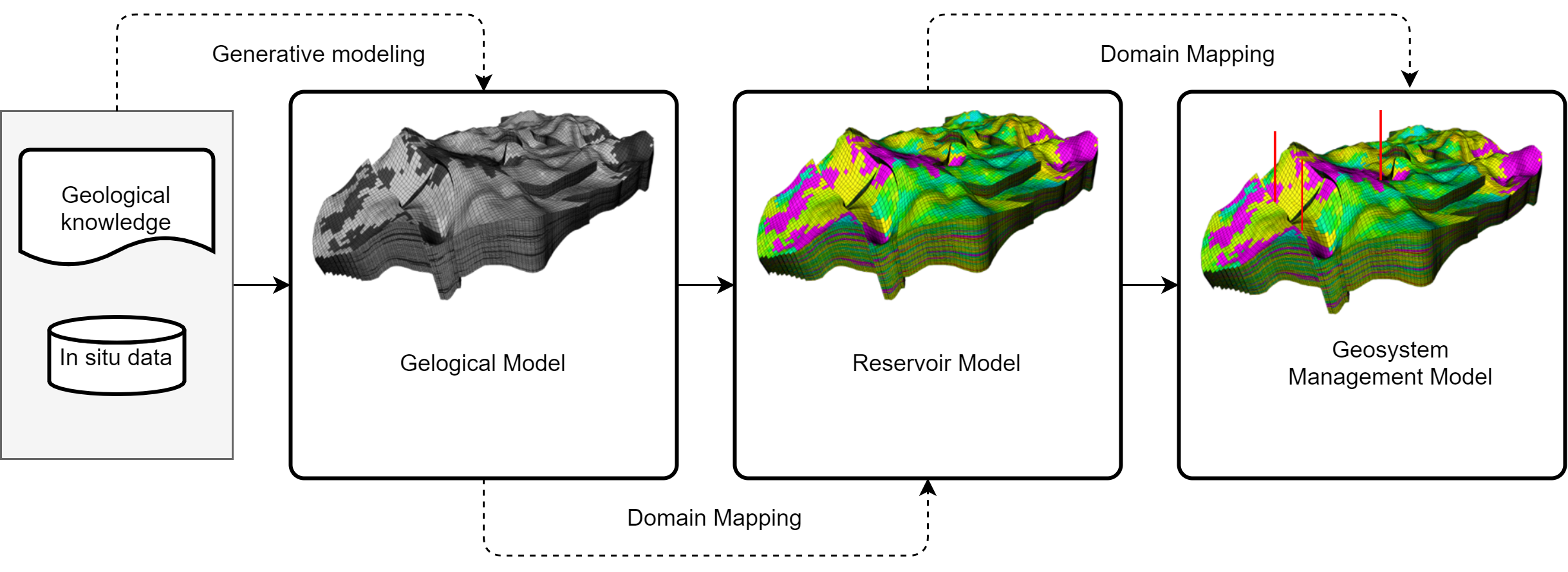
Figure 1: The conventional subsurface modeling workflow consists of (from left to right) data collection and interpretation, geological modeling, fluid modeling, and system modeling. Machine learning has potential to automate all of these steps.

We argue that subsurface modeling is inherently a semisupervised generative modeling process (Chapelle et al., 2009), in which joint data distributions are learned via limited observations. A main difference is that in field-scale subsurface modeling, observations are always sparse and only indirectly related to data. For example, the observed quantities may be well logs, but the data of interest are fluid saturation and pore pressure (state variables); in this case, well logs are first analyzed to infer stratigraphy and parameter distributions (e.g., porosity and permeability), which are then mapped to predictions of the state variables. Physics-based modeling serves two purposes throughout this process, namely, mapping the parameter space to state space, and providing a spatiotemporal interpolation/extrapolation mechanism that is guided by first principles and prior knowledge. A main issue of this traditional workflow is that a significant amount of human processing time and computational time is involved, limiting its efficiency and potentially introducing significant latency and subjectivity during the process. On the other hand, machines are good at automating processes and learning proxy models after getting trained. Tremendous opportunities now exist to integrate physics-based modeling and data-driven ML to improve the accuracy and efficacy of the geoanalytics workflow.

To help the geoscientific community better embrace and incorporate various ML methods, this chapter provides a survey of recent physics-based ML developments in geosciences, with a focus on three main aspects—a taxonomy of ML methods that have been used (Section 2), brief introduction to some of the commonly used ML methods 3), the types of use cases that are amenable to physics-based ML treatment (Section 4 and Table 2), and finally challenges and future directions of ML applications in geosystem modeling (Section 5).

2 Taxonomy of GeoML Methods

Table 1 lists the main notations and symbols used in this survey.

Table 1: Notations and symbols used in this survey.

Notations	Descriptions
${\bf{A}}$	adjacency matrix
${\bf{b}}$	bias vector
$d$	number of features
$\mathcal{D}$	discriminative network
${\bf{D}}$	node degree matrix
$\mathbb{E}$	expectation operator
$\mathcal{E}$	graph edge set
$\mathcal{G}$	generative network
${\bf{I}}$	identity matrix
${\bf{L}}$	graph Laplacian
$\mathcal{I}$	prior information
$n$	number of samples
$N$	number of nodes in a graph
$p(\cdot)$	probability distribution
$\mathcal{V}$	graph node set
${\bf{W}}$	weight matrix
${\bf{x}}\in{\mathbb{R}}^{d}$	feature vector
$\hat{{\bf{x}}}\in\mathbb{R}^{d}$	estimated feature vector
$X\in\mathbb{R}^{d}$	feature variable
$y$	label, target variable, state variable
${\bf{d}}^{obs}$	data vector
${\bf{z}}$	latent space vector
$\theta$	parameters

Physics-based ML in the geoscientific domain (hereafter GeoML) is a type of scientific machine learning (SciML) which, in turn, may be considered a special branch of AI/ML that develops applied ML algorithms for scientific discovery, with special emphases on domain knowledge integration, data interpretation, cross-domain learning, and process automation (Baker et al., 2019). A main thrust behind the current SciML effort is to combine the strengths of physics-based models with data-driven ML methods for better transparency, interpretability, and explainability (Roscher et al., 2020). Unless otherwise specified, we shall use the terms physics-based, process-based, and mechanistic models interchangeably in this survey.

We provide three taxonomies of GeoML methods based on their design and use. First, existing GeoML methods may be classified according to the widely used ML taxonomy into unsupervised, supervised, and reinforcement learning methods. In Figure 2, this taxonomy is used to group the existing GeoML applications, an exposition of which will be deferred to Section 4.

Another commonly used taxonomy is generative models vs. discriminative models. Generative models seek to learn the probability distributions/patterns of individual classes in a dataset, while discriminative models try to predict the boundary between different classes in a dataset (Goodfellow et al., 2016). Thus, in a supervised learning setting and for given training samples of input variables $X$ and label $y$, $\{({\bf x}_{i},y_{i})\}$, a generate model learns the joint distribution $p(X,y)$ so that new realizations can be generated, while a discriminative model learns to predict the conditional distribution $p(y\mid X)$ directly. Generative models can be used to learn from both labeled and unlabeled data in supervised, unsupervised, or supervised tasks, while discriminative models cannot learn from unlabeled data, but tend to outperform their generative counterparts in supervised tasks (Chapelle et al., 2009). In GeoML, generative models are particularly appealing because of the strong need for understanding the causal relationships, and because the same underlying Bayesian frameworks are also employed in many physics-based frameworks. In the classic Bayesian inversion framework, for example, the parameter inference problem may be cast as (Sun and Sun, 2015),

$$p(\theta\mid{\bf d}^{obs},\mathcal{I})=\frac{p(\theta\mid\mathcal{I})p({\bf d}^{obs}\mid\theta,\mathcal{I})}{p({\bf d}^{obs}\mid\mathcal{I})},$$ (1)

where the posterior distribution of model parameters $\theta$ are inferred from the state observations ${\bf d}^{obs}$ and prior knowledge $\mathcal{I}$. Many physics-based ML applications exploit the use of ML models for estimating the same distributions, but by fusing domain knowledge to form priors and constraints.

On the basis of how physical laws and domain knowledge are incorporated, existing GeoML methods fall into pre-training, physics-informed training, residual modeling, and hybrid learning methods.

In pre-training methods, which are widely used in ML-based surrogate modeling, prior knowledge and process-based models are mainly used to generate training samples for ML from limited real information. The physics is implicitly embedded in the training samples. After the samples are generated, an ML method is then used to learn the unknown mappings between parameters and model states through solving a regression problem. In physics-informed training, physics laws and constraints are utilized explicitly to formulate the learning problem, such that ML models can reach a fidelity on par to PDE-based solvers. Residual modeling methods use ML as a fine-tuning, post-processing step, under the assumption that the process-based models reasonably capture the large-scale “picture” but have certain missing processes, due to either conceptual errors or unresolved/unmodeled processes (e.g., subgrid processes). ML models are then trained to learn the mapping between model inputs and error residuals (e.g., between model outputs and observations), which are used to correct the effect of missing processes on model outputs (Sun et al., 2019a; Reichstein et al., 2019). A main caveat of the existing ML paradigm is that models are trained offline using historical data, and then deployed in operations, in the hope that the future environment stays more or less under the same conditions. This is referred to as the closed-world assumption, namely, classes of all new test instances have already been seen during training (Chen and Liu, 2018). In some situations, new classes of data may appear or the environment itself may drift over time; in other situations, it is desirable to adapt a model trained on one task to other similar tasks without training separate models. Hybrid learning methods focus on continual or lifelong learning, in which ML models and process-based models co-evolve to reflect new information available. The past knowledge is accumulated and then used to help future learning (Chen and Liu, 2018; Parisi et al., 2019). Hybrid learning methods thus have elements of multitask learning, transfer learning, and reinforcement learning from the ML side, and data assimilation from the process modeling side. Understandably hybrid learning models are more difficult to formulate and train, but they represent important steps toward the “real” AI, in which agents learn to act reasonably well not in a single domain but in many domains (Bostrom and Yudkowsky, 2014).

3 Commonly Used GeoML Algorithms

For completeness, we briefly review the common algorithms and application frameworks behind the GeoML use cases to be covered in Section 4 (see also Table 2). Most of the categories mentioned herein are not exclusive. Autoencoders, the generative adversarial networks, and graph neural networks are high-level ML algorithmic categories that include many variants, while spatial-temporal methods and physics-informed methods are application frameworks that may be implemented using any of the ML methods.

3.1 Autoencoders

A main premise of the modern AI/ML is in representation learning, which seeks to extract the low-dimensional features or to disentangle the underlying factors of variation from learning subjects that can support generic and effective learning (Bengio et al., 2013). An important class of methods for representation learning is autoencoders, which are unsupervised learning methods that encode unlabeled input data into low-dimensional embeddings (latent space variables) and then reconstruct the original data from the encoded information. For input data ${\bf x}$, the encoder maps it to a latent space vector, ${\bf z}=f({\bf x};{\bf W}_{e})$, while the decoder reconstructs the input data, $\hat{{\bf x}}=g({\bf z};{\bf W}_{d}),$where ${\bf W}_{e}$ and ${\bf W}_{d}$ are weight matrices of the encoder and decoder, respectively. The standard autoencoder is trained by minimizing the reconstruction error, which implies a good representation should keep the information of the input data well. Once trained, the autoencoder may serve as a generative model (prior) for generating new samples, clustering, or for dimension reduction. Variants of autoencoders include variational autoencoder (VAE) and restricted Boltzmann machine (RBM) (Goodfellow et al., 2016; Doersch, 2016).

It is worth pointing out that the notion of representation learning has long been investigated in the context of parameterization and inversion of physics-based models, although the primary goal there is to make the inversion process less ill-posed by reducing the degree of unknowns. In geosciences, autoencoders are closely related to stochastic geological modeling, which is the main subject of study in geostatistics (Journel and Huijbregts, 1978). In stochastic geological modeling, the real geological formation is considered one realization of a generative stochastic process that can only be “anchored” through a limited set of measurements. The classic principle component analysis (PCA) may be used to encode statistically stationary random processes, while other algorithms, such as the multipoint statistics simulators, have been commonly used to simulate more complex depositional environments (Caers and Zhang, 2004; Mariethoz et al., 2010). Autoencoders, when implemented using the deep convolutional neural nets (CNNs) (Chan and Elsheikh, 2017; Yoon et al., 2019), provide a more flexible tool for parameterizing the complex geological processes and for generating (synthetic) training samples for the downstream tasks, such as surrogate modeling. From this sense, autoencoders fall in the category of pre-training methods.

3.2 Generative adversarial networks

The generative adversarial networks (GANs), introduced originally in (Goodfellow et al., 2014), have spurred strong interests in geosciences. The vanilla GAN (Goodfellow et al., 2014) trains a generative model (or generator) and a discriminator model (discriminator) in a game theoretic setting. The generator $\mathcal{\hat{{\bf x}}=G}({\bf z};{\bf W}_{g})$ learns the data distribution and generates fake samples, while the discriminator $\mathcal{D}({\bf x};{\bf W}_{d})$ predicts the probability of fake samples being from the true data distribution, where ${\bf W}_{g}$ and ${\bf W}_{d}$ are trainable weight matrices. A minimax optimization problem is formulated, in which the generator is trained to minimize the reconstruction loss to generate more genuine samples, while the discriminator is trained to maximize its probability of distinguishing true samples from the fake samples,

$$\text{arg}\underset{\mathcal{G}}{\min}\underset{\mathcal{D}}{\max}\mathbb{E}_{{\bf x}\sim p_{data}({\bf x})}\log[\mathcal{D}({\bf x};{\bf W}_{d})]+\mathbb{E}_{{\bf z}\sim p({\bf z})}\log[1-\mathcal{D}(\mathcal{G}({\bf z};{\bf W}_{g});{\bf W}_{d})],$$ (2)

where $p_{data}(\cdot)$ and $p_{{\bf z}}(\cdot)$ are data and latent variable distributions. In practice, the generator and discriminator are trained in alternating loops, the weights of one model is frozen when the weights of the other are updated. It has been shown that if the discriminator is trained to optimality before each generator update, minimizing the loss function is equivalent to minimizing the Jensen-Shannon divergence between data $p_{data}(\cdot)$ and generator $p_{{\bf\hat{x}}}(\cdot)$ distributions (Goodfellow et al., 2016).

Many variants of the vanilla GAN have been proposed, such as the deep convolutional GAN (DCGAN)(Radford et al., 2015), superresolution GAN (SRGAN) (Ledig et al., 2017), Cycle-GAN (Zhu et al., 2017), StarGAN (Choi et al., 2018), and missing data imputation GAN (GAIN) (Yoon et al., 2018). Recent surveys of GANs are provided in (Creswell et al., 2018; Pan et al., 2019). So far, GANs have demonstrated superb performance in generating photo-realistic images and learning cross-domain mappings. Training of the GANs, however, are known to be challenging due to (a) larger-size networks, especially those involving a long chain of CNN blocks and multiple pairs of generators/discriminators, (b) the nonconvex cost functions used in GAN formulations, (c) diminished gradient issue, namely, the discriminator is trained so well early on in training that the generator’s gradient vanishes and learns nothing, and (d) the “mode collapse” problem, namely, the generator only returns samples from a small number of modes of a mutimodal distribution (Goodfellow et al., 2016). In the literature, different strategies have been proposed to alleviate some of the aforementioned issues. For example, to adopt and modify deep CNNs for improving training stability, the DCGAN architecture (Radford et al., 2015) was proposed by including stride convolutions and ReLu/LeakyRelu activation functions in the convolution layers. To ameliorate stability issues with the GAN loss function, the Wasserstein distance was introduced in the Wasserstein GAN (WGAN) (Arjovsky et al., 2017; Gulrajani et al., 2017) to measure the distance between generated and real data samples, which was then used as the training criterion in a critic model. To remedy the mode collapse problem, the multimodal GAN (Huang et al., 2018) was introduced, in which the latent space is assumed to consist of domain-invariant (called content code) and domain specific (called style code) parts; the former is shared by all domains, while the latter is only specific to one domain. The multimodal GAN is trained by minimizing the image space reconstruction loss, and the latent space reconstruction loss. In the context of continual learning, the memory replay GAN (Wu et al., 2018) was proposed to learn from a sequence of disjoint tasks. Like the autoencoders, GAN represents a general formulation for supervised and semi-supervised learning, thus its implementation is not restricted to certain types of network models.

3.3 Graph neural networks

ML methods originating from the computer vision typically assume the data has a Euclidean structure (i.e., grid like) or can be reasonably made so through resampling. In many geoscience applications, data naturally exhibits a non-Euclidean structure, such as the data related to natural fracture networks and environmental sensor networks, or the point cloud data obtained by lidar. These unstructured data types are naturally represented using graphs. A graph $\mathcal{G}$ consists of a set of nodes $\mathcal{V}$ and edges $\mathcal{E}$, $\mathcal{G}=(\mathcal{V},\mathcal{E})$. Each node $v_{i}\in\mathcal{V}$ is characterized by its attributes and has a varying number of neighbors, while each edge $e_{ij}\in\mathcal{E}$ denotes a link from node $v_{j}$ to $v_{i}$. The binary adjacency matrix ${\bf A}$ is used to define graph connections, with its elements $a_{ij}=1$ if there is edge between $i$ and $j$ and $a_{ij}=0$ otherwise.

Various graph neural networks (GNNs) have been introduced in recent years to perform ML tasks on graphs, a problem known as “geometric learning” (Bronstein et al., 2017). The success (e.g., efficiency over deep learning problems) of CNN is owed to several nice properties in its design, such as shift-invariance and local connectivity, which lead to shared parameters and scalable networks (Goodfellow et al., 2016). A significant endeavor in the GNN development has been related to extending these CNN properties to graphs using various clever tricks.

The graph convolutional neural networks (GCNN) extend CNN operations to non-Euclidean domains and consist of two main classes of methods, the spectral-based methods and the spatial-based methods. In spectral-based methods, the convolution operation is defined in the spectral domain through the normalized graph Laplacian, ${\bf L}$, defined as

$${\bf L}={\bf I}-{\bf D}^{-1/2}{\bf A}{\bf D}^{-1/2}={\bf U}{\bf\varLambda}{\bf U^{T}},$$ (3)

where ${\bf A}$ is adjacency matrix, ${\bf I}$ is identify matrix, ${\bf D}$ is the node degree matrix (i.e, $d_{ii}=\sum_{j}a_{ij}$), and ${\bf U}$ and $\Lambda$ are eigenvector matrix and diagonal eigenvalue matrix of the normalized Laplacian. Utilizing ${\bf U}$ and $\Lambda$, the spectral graph convolution on input ${\bf x}$ is defined by a graph filter ${\bf g}_{\theta}$ (Bruna et al., 2013)

$${\bf g_{\theta}}*{\bf x}={\bf U}{\bf g}_{\theta}(\Lambda){\bf U}^{T}{\bf x},$$ (4)

where $*$ denotes the graph convolution operator and the graph filter ${\bf g}_{\theta}(\Lambda)$ is parameterized by the learnable parameters $\theta_{ij}$. Main limitations of the original graph filter given in Eqn. 4 are it is non-local, only applicable to a single domain (i.e., fixed graph topology), and involves the computationally expensive eigendecomposition ($O(N^{3})$ time complexity) (Bronstein et al., 2017; Wu et al., 2020). Later works proposed to make the graph filter less computationally demanding by approximating ${\bf g}_{\theta}(\Lambda)$ using the Chebychev polynomials of $\Lambda$, which led to ChebNet (Defferrard et al., 2016) and Graph Convolutional Net (GCN) (Kipf and Welling, 2016). It can be shown these newer constructs lead to spatially localized filters, such that the number of learnable parameters per layer does not depend upon the size of the input (Bronstein et al., 2017). In the case of GCN, for example, the following graph convolution operator was proposed (Kipf and Welling, 2016),

$${\bf g_{\theta}*x}\approx\theta\left({\bf I}+{\bf D}^{-1/2}{\bf A}{\bf D}^{-1/2}\right){\bf x}=\theta\left(\tilde{{\bf D}}^{-1/2}{\bf\tilde{A}}{\bf\tilde{D}}^{-1/2}\right){\bf x},$$ (5)

where $\theta$ is a set of filter parameters, and a renormalization trick was applied in the second equality in Eqn. 5 to improve the numerical stability, ${\bf\tilde{A}=A+I}$ and $\tilde{d}_{ii}=\sum_{j}\tilde{a}_{ij}$. The above graph convolutional operation can be generalized to multichannel inputs ${\bf X}\in\mathbb{R}^{N\times C}$, such that the output is given by $\tilde{{\bf D}}^{-1/2}{\bf\tilde{A}}{\bf\tilde{D}}^{-1/2}{\bf X}\Theta$, where $\Theta$ is a matrix of filter parameters.

In spatial-based methods, graph convolution is defined directly over a node’s local neighborhood, instead via the eigendecomposition of Laplacian. In diffusion CNN (DCNN), information propagation on a graph is modeled as a diffusion process that goes from one node to its neighboring node according to a transition probability (Atwood and Towsley, 2016). The graph convolution in DCNN is defined as

$${\bf H}^{(k)}=\sigma\left({\bf W}^{(k)}\circ{\bf P}^{k}{\bf X}\right),\;k=1,\dots,K,$$ (6)

where ${\bf X}$ is input matrix, ${\bf P}={\bf D}^{-1}{\bf A}$ is transition probability matrix, $k$ defines the power of ${\bf P}$, $K$ is the total number of power terms used (i.e., the number of hops or diffusion steps) in the hidden state extraction, and ${\bf W}$ and ${\bf H}$ are the weight and hidden state matrices, respectively. The final output is obtained by concatenating the hiddden state matrices and then passing to an output layer. In GraphSAGE (Hamilton et al., 2017) and message passing neural network (MPNN) (Gilmer et al., 2017), a set of aggregator functions are trained to learn to aggregate feature information from a node’s local neighborhood. In general, these networks consist of three stages, message passing, node update, and readout. That is, for each node $v$ and at the $k\text{-th}$ iteration, the aggregation function $f_{k}$ combines the node’s hidden representation with those from its local neighbors $\mathcal{N}(v)$, which is then passed to update functions to generate the hidden states for the next iteration,

$${\bf h}_{v}^{(k)}=\sigma\left({\bf W}^{(k)},f_{k}\left({\bf h}_{v}^{(k-1)},\left\{{\bf h}_{u}^{(k-1)},u\in\mathcal{N}(v)\right\}\right)\right),$$ (7)

where ${\bf h}$ denotes a hidden-state vector. Finally, in the readout stage, a fixed-length feature vector is computed by a readout function and then passed to a fully connected layer to generate the outputs.

In general, spatial-based methods are more scalable and efficient than the spectral methods because they do not involve the expensive matrix factorization, the computation can be performed in mini-batches and, more importantly, the local nature indicates that the weights can be shared across nodes and structures (Wu et al., 2020). Counterpart implementations of all well-established ML architectures (e.g., GAN, autoencoder, and RNN) can now be found in GNNs. Recent reviews on GNNs can be found in (Zhou et al., 2018; Wu et al., 2020).

For subsurface applications, a main challenge is related to graph formulation, namely, given a set of spatially discrete data, how to connect the nodes. Common measures calculate certain pairwise distances (e.g., correlation, Euclidean, city block), while other methods incorporate the underlying physics (e.g., discrete fracture networks (Hyman et al., 2018)) to identify the graphs.

3.4 Spatiotemporal ML methods

In this and the next subsection, we review two methodology categories that use one or more of the aforementioned methods as construction blocks. Spatiotemporal processes are omnipresent in geosystems and represent an important area of study (Kyriakidis and Journel, 1999). For gridded image-like data, the problem bears similarity to the video processing problem in computer vision. In general, two classes of ML methods have been applied, those involving only CNN blocks and those combining with recurrent neural nets (RNNs).

Fully-connected CNNs can be used to model temporal dependencies by stacking the most recent sequence of images/frames in a video stream. In the simplest case, the channel dimension of the input tensor is used to hold the sequence of images and CNN kernels are used to extract features like in a typical CNN-based model (i.e., 2D kernels for a stack of 2D images). In other methods, for example, C3D (Tran et al., 2015) and temporal shift module (TSM) (Lin et al., 2019), an extra dimension is added to the tensor variable to help extract temporal patterns. C3D uses 3D CNN operators, which generally leads to much larger networks. TSM was designed to shift part of the channels along the temporal dimension, thus facilitating information extraction from neighboring frames while adding almost no extra computational costs compared to the 2D CNN methods (Lin et al., 2019).

The hybrid methods use a combination of RNNs with CNNs, using the former to learn long-range temporal dependencies and the latter to extract hierarchical features from each image. The convolutional long short-term memory (ConvLSTM) network (Shi et al., 2015) represents one the most well known methods under this category. In ConvLSTM, features from convolution operations are embedded in the LSTM cells, as described by the following series of operations (Shi et al., 2015)

$${\bf i}_{t} = \sigma\left({\bf W}_{xi}*{\bf X}_{t}+{\bf W}_{hi}*{\bf H}_{t-1}+{\bf W}_{ci}\circ{\bf C}_{t-1}+{\bf b}_{i}\right),$$

$${\bf f}_{t} = \sigma\left({\bf W}_{xf}*{\bf X}_{t}+{\bf W}_{hf}*{\bf H}_{t-1}+{\bf W}_{cf}\circ{\bf C}_{t-1}+{\bf b}_{f}\right),$$

$${\bf C}_{t} = {\bf f}_{t}\circ{\bf C}_{t-1}+{\bf i}_{t}\circ\tanh\left({\bf W}_{xc}*{\bf X}_{t}+{\bf W}_{hc}*{\bf H}_{t-1}+{\bf b}_{c}\right),$$ (8)

$${\bf o}_{t} = \sigma\left({\bf W}_{xo}*{\bf X}_{t}+{\bf W}_{ho}*{\bf H}_{t-1}+{\bf W}_{co}*{\bf C}_{t}+{\bf b}_{o}\right),$$

$${\bf H}_{t} = {\bf o}_{t}\circ\tanh({\bf C}_{t}),$$

where ${\bf X}$, ${\bf H}$, and ${\bf C}$ are input, hidden, and cell output matrices, ${\bf W}$ and ${\bf b}$ represent learnable weights and biases, $\sigma$ and tanh denote activation functions, and ${\bf i}$, ${\bf f},$and ${\bf o}$ are the input, forget, and output gates. The symbols $*$ and $\circ$ denote the convolution operator and Hadamard (element-wise) product, respectively. Because of its complexity and size, ConvLSTM networks may be more difficult to train than the CNN-only methods.

Geological processes are known to exhibit certain correlation in space and time. The convolution operations are like a local filter and not good at catching large scale features, which is especially the case for relatively shallow CNN-based models. In recent years, attention mechanisms have been introduced to better capture the long-range dependencies in space and time, and to give higher weight to most relevant information (Vaswani et al., 2017). In the location-based attention mechanism, for example, input feature maps are transformed and used to calculate a location-dependent attention map (Wang et al., 2018; Zhang et al., 2019)

$${\bf F} = {\bf W}_{f}*{\bf X}_{i},\;{\bf G}={\bf W}_{g}*{\bf X}_{j},$$ (9)

$$\alpha_{ji} = \frac{\exp(s_{ij})}{\sum_{i=1}^{N}\exp(s_{ij})},\;s_{ij}={\bf F}^{T}{\bf G}$$ (10)

$${\bf O}_{j} = \sum_{i=1}^{N}\alpha_{ji}({\bf W}_{h}*{\bf X}_{i}),$$ (11)

where ${\bf{\bf X}}\in\mathcal{\mathbb{R}}^{C\times H\times W}$ are the input feature maps, $C$, $H$, and $W$ are the channel and spatial dimensions of the input feature map, $N=CW$ is the total number of features in the feature map, ${\bf F}$ and ${\bf G}$ are two transformed feature maps obtained by passing the inputs to separate $1\times 1$ convolutional layers, and the attention weights $\alpha_{ji}$ measure the influence of remote location $i$ on region $j$. The resulting attention map is then concatenated with the input feature maps to give the final outputs from the attention block. A similar attention mechanism may be defined for the temporal dimension to catch the temporal correlation (Zhu et al., 2018). The attention-based ML models thus offer attractive alternatives to many parametric geostatistical methods for 4D geoprocess modeling.

For unstructured data, GNNs can be used to learn spatial and temporal relationships. For example, spatiotemporal graph convolution network (ST-GCN) and spatiotemporal multi-graph convolution network (Geng et al., 2019) were used for skeleton-based action recognition and for ride share forecast, respectively. The spatial-based GNNs may also be suitable for the missing data problem, where the neighborhood information can be used to estimate missing nodal values. For problems that can be treated using GNNs, the resulting learnable parameter sizes are generally much smaller.

3.5 Physics-informed methods

As mentioned in the last subsection, all GeoML applications that incorporate certain domain knowledge or use process-based models in the workflow may be considered physics informed. Recently, a number of SciML frameworks have been developed to incorporate the governing equations in a more principled way. In general, these methods may be divided into finite-dimensional mapping methods, neural solver methods, and neural integral operator methods (Li et al., 2020). All these methods seek to either parameterize the solution of a PDE, $u=\mathcal{M}(a)$, where $\mathcal{M}$ is model operator, $u\in\mathcal{U}$ is the solution and $a\in\mathcal{A}$ are parameters, or to approximate the model operator itself.

Finite-dimensional methods learn mappings between finite-dimensional Euclidean spaces (e.g., the discretized parameter space and solution space), which is similar to many use cases in computer vision. The main difference is that additional PDE loss terms related to the PDE being solved are incorporated. For example, Zhu et al. (2019) considered the steady-state flow problem in porous media (an elliptic PDE) and used the variational form of the PDE residual as a loss term, in addition to the data mismatch term. Many of the existing methods (e.g., U-Net) from the computer vision can be directly applied in these methods. A main limitation of the finite-dimensional methods is they are grid specific (without resampling) and problem specific.

In neural solver methods, such as physics-informed neural networks (PINNs) (Raissi et al., 2019; Zhu et al., 2019; Lu et al., 2019), universal differential equation (UDE) (Rackauckas et al., 2020), and PDE-Net (Long et al., 2019), the neural networks (differentiable functions by design) are used to approximate the solution and the PDE residual is derived for the given PDE by leveraging auto differentiation and neural symbolic computing. In general, these approaches assume the PDE forms/classes are known a priori, although some approaches (e.g., PDE-Net) can help to identify whether certain terms are present in a PDE or not under relatively simple settings.

The neural integral operator methods (Fan et al., 2019; Winovich et al., 2019; Li et al., 2020) parameterize the differential operators (e.g., Green’s function, Fourier transform) resulting from the solution of certain types of PDEs. These methods are mesh independent and learn mappings between infinite-dimensional spaces. In other words, a trained model has the “super-resolution” capability to map from a low-dimensional grid to a high-dimensional grid.

All the physics-informed methods may provide accurate proxy models. The advantages of these differential equation oriented methods are (a) smooth solutions, by enforcing derivatives as constraints they effectively impose smoothness in the solution, (b) extrapolation, by forcing the NN to replicate the underlying differential equations these methods also inherit the extrapolation capability of physics-based models, which is lacking in purely data-driven methods, (c) closure approximations, by parameterizing the closure terms using hidden neurons they allow the unresolved processes to be represented and “discovered” in the solution process, and (d) less data requirements, which comes as the result of the extensive constraints used in those frameworks. On the other hand, the starting point of many methods are differential equations, which means extensive knowledge and analysis are still required to select and formulate the equations, a process that is well known for its equifinality issue (Beven and Freer, 2001). Future works are still required to make the physics-informed methods less PDE-class specific and be able to handle flexible initial/boundary conditions and forcing terms.

4 Applications

The number of GeoML publications has grown exponentially in recent years. Here we review a selected set of recent GeoML applications according to the taxonomy discussed under Section 2, and plotted in Fig. 2. The list of publications is also summarized in Table 2, according to their ML model class, model type, use case, and the way physics was incorporated. In making the list, we mainly focused on reservoir-scale studies. Reviews of porous flow ML applications in other disciplines (e.g., material science and chemistry) can be found in (Alber et al., 2019; Brunton et al., 2020).

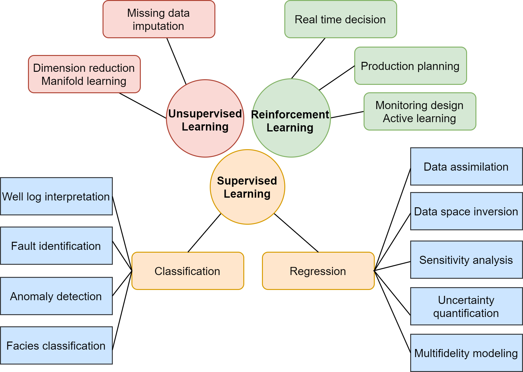
Figure 2: Common ML applications in geosciences may be grouped under unsupervised, supervised, and reinforcement learning.

Early works adopting the deep learning methods explored their strong generative modeling capability for geologic simulation. In (Chan and Elsheikh, 2017), WGAN was used to generate binary facies realizations (bimodal). Training samples were generated using a training image, which has long been used in multipoint geostatistics as a geology-informed guide for constraining image styles (Strebelle, 2002). WGAN was trained to learn the latent space encoding of the bimodal facies field. The authors showed that WGAN achieved much better performance than PCA, which is a linear feature extractor that works best on single-modal, Gaussian-like distributions. In (Liu et al., 2019), a convolutional encoder was trained to reconstruct a complex geologic model from its PCA parameterization. A key idea there was to learn the mismatch between the naïve PCA representations and the original high-fidelity counterparts such that new high-resolution realizations can be generated using latent variables obtained from PCA. Recently, DCGANs have been applied to generate drainage networks by transforming the training network images to directional information of flow on each node of the network (Kim et al., 2020). The generated network has been dramatically improved by optimal decomposition of the drainage connectivity information into multiple binary layers with the connectivity constraints stored.

A large number of GeoML applications fall under surrogate modeling, which is not surprising given that the geocommunity has long been utilizing surrogate models in model-based optimization, sensitivity analysis, and uncertainty quantification (Forrester and Keane, 2009; Razavi et al., 2012). Because reservoir models are 2D or 3D distributed models, many ML studies entailed some type of end-to-end, cross-domain learning architecture, which translates an image of input parameter to state variable maps. In general, these methods utilize physics-based porous flow models to generate training samples. In (Mo et al., 2019b), a convolutional autoencoder was trained to learn the cross-domain mapping between permeability maps and reservoir states (pressure and saturation distributions) at different times. In (Zhong et al., 2019, 2020a), a U-Net based convolutional GAN was trained to solve a similar problem. Both studies also demonstrated the strong skill of ML-based models in uncertainty quantification. In Tang et al. (2020), a hybrid U-Net and ConvLSTM model was trained to learn the dynamic mappings in multiphase reservoir simulations. In (Mo et al., 2020), multi-level residual learning blocks were used to implement a GAN model for surrogate modeling. ML techniques have also been combined with model reduction techniques (e.g., proper orthogonal decomposition or POD) to first reduce the dimension of models states before applying ML (Jin et al., 2020). The Darcy’s flow problem has also been used as a classic test case in many physics-informed studies, but generally under relatively simple settings (Zhu et al., 2019; Winovich et al., 2019; Li et al., 2020)

Model calibration and parameter estimation represent an integral component of the closed-loop geologic modeling workflow. A general strategy has been using autoencoders to parameterize the model parameters as random fields, the resulting latent variables are then “calibrated” using observation data in an outer-loop optimization, such as Markov chain Monte Carlo (Laloy et al., 2018) and ensemble smoothers (Canchumuni et al., 2019; Liu et al., 2019; Mo et al., 2020; Liu and Grana, 2020). In Bayesian terms, this workflow yields the so-called conditional realizations of the uncertain parameters, which are simply samples of a posterior distribution informed by observations and priors (see Eqn 1). Other studies approached the inversion problem directly using cross-domain mapping. For example, DiscoGAN and CycleGAN were used to learn bidirectional (Sun, 2018; Wu and Lin, 2019) and tri-directional mappings (Zhong et al., 2020b).

Many process-based models are high-dimensional and expensive to run, prohibiting the direct use of cross-domain surrogate modeling. ML-based multifidelity modeling offers an intermediate step. The general idea is to reduce the requirements on high-fidelity model runs by utilizing cheaper-to-run, lower fidelity models. Towards this goal, in (Perdikaris et al., 2017), a recursive Gaussian process was trained sequentially using data from multiple model fidelity levels, reducing the number of high-fidelity model runs. In (Meng and Karniadakis, 2020), a multifidelity PINN was introduced to learn mappings (cross-correlations) between low- and high-fidelity models, by assuming the mapping function can be decomposed into a linear and a nonlinear part. Their method was expanded using Bayesian neural networks to not only learn the correlation between low- and high-fidelity data, but also give uncertainty quantification (Meng et al., 2020).

Fractures and faults are extensively studied in geosystem modeling for risk assessment and production planning. In (Schwarzer et al., 2019), a recurrent GNN was used to predict the fracture propagation, using simulation samples from high-fidelity discrete fracture network models. In (Sidorov and Yngve Hardeberg, 2019), GNN was used to extract crack patterns directly from high-resolution images, which may have a significant implication to a wide range of geological applications.

Ultimately, the goal of geosystem modeling is to train ML agents to quickly identify optimal solutions and/or policies, which is a challenging problem that requires integrating many pieces in the current ML ecosystems. The recently advanced deep reinforcement learning algorithms offer a new paradigm for exploiting past experiences while exploring new solutions (Mnih et al., 2013). In general, model-based deep reinforcement learning frameworks solve a sequential decision making problem. At any time, the agent chooses a trajectory that maximizes the future rewards. Doing so would require hopping many system states in the system space, which is challenging for high-dimensional systems. In (Sun, 2020), the deep Q learning (DQL) algorithm was used to identify the optimal injection schedule in a geologic carbon sequestration planning. A deep surrogate, autoregressive model was trained using U-Net to facilitate state transition prediction. A discrete planning horizon was assumed to reduce the total computational cost. In (Ma et al., 2019), a set of deep reinforcement learning algorithms were applied to maximize the net present value of water flooding rates in oil reservoirs. It remains a challenge to generate the surrogate models for arbitrary state transitions, such as that is encountered in well placement problems where both the number and locations of new wells need to be optimized.

Table 2: List of physics-informed GeoML applications

Model class	Model Name	Use Case	Physics Used	Citation
Autoencoder	Conv-VAE	Geologic simulation	Geology	(Laloy et al., 2018), (Canchumuni et al., 2019)
	CNN-PCA	Geologic simulation	Geology, reservoir model	(Liu et al., 2019)
	Conv-AE	Surrogate modeling	Reservoir model outputs	(Mo et al., 2019b),(Mo et al., 2019a)
	CNN	Model reduction, surrogate modeling	Multiphase flow model	(Wang and Lin, 2020)
Generative adversarial networks	WGAN	Unconditional geologic simulation	Geology	(Chan and Elsheikh, 2017)
	DiscoGAN	Bidirectional parameter-state mapping	Groundwater model outputs	(Sun, 2018)
	Conditional GAN	Surrogate modeling	Reservoir model outputs	(Zhong et al., 2019),(Zhong et al., 2020a)
	ConvGAN	Inversion	Geology, groundwater model	(Mo et al., 2020)
	CycleGAN	Tridirectional parameter-state mapping	Multiphase flow, petrophysics	(Zhong et al., 2020b)
	CycleGAN	Bidirectional parameter-state mapping	Full waver inversion	(Wu and Lin, 2019),(Wang et al., 2019)
	DCGAN	Drainage networks	Hydraulic connectivity	(Kim et al., 2020)
Graph neural nets	Diffusion GNN	Discrete fracture modeling	Fracture connectivity	(Schwarzer et al., 2019), (Sidorov and Yngve Hardeberg, 2019)
Spatiotemporal	Unet-LSTM	Surrogate modeling	Reservoir model outputs	(Tang et al., 2020)
	CNN only	Surrogate modeling	Reservoir model	(Zhong et al., 2019), (Mo et al., 2019b)
PDE-informed	DNN	Parameter estimation	Soil physics	(Tartakovsky et al., 2020)
	DNN	Forward modeling and inversion	Soil physics	(bekele2020physics)
	Conv-AE	Surrogate modeling	Flow equation	(Zhu et al., 2019)
	DNN	Immsicible flow modeling	Reservoir flow equation	(Fuks and Tchelepi, 2020)
	Neural operator	Surrogate modeling	Darcy flow equation	(Li et al., 2020)

5 Challenges and Future Directions

Our survey shows that GeoML has opened a new window for tackling longstanding problems in geological modeling and geosystem management. Nevertheless, a number of challenges remain, which are described below.

Training data availability

GeoML tasks require datasets for training, validation, and testing. In the subsurface domain, data acquisition can be costly. For example, to acquire 3D seismic data, an operator may spend at least $1M before seeing results. The costs of drilling new exploration wells are on the same order of magnitudes. Thus, data augmentation using synthetic datasets will play an important role in improving the current generalization capability of ML models. A main challenge is related to generating realistic datasets that also meet unseen field conditions. In addition, generating simulation data for subsurface applications can also be time consuming if the parameter search space is large and requires substantial computational resources.

Efforts from the public and private sectors have started to make data available. Government agencies encourage or require oil and gas operators to regularly report well information (e.g., drilling, completion, plugging, production, etc.) and make the data available to the public. Standing on the foundation, companies integrate the data and added proprietary assessments for commercial licenses. The U.S. Energy Information Administration (EIA) implements multiple approaches to facilitate data access (https://www.eia.gov/opendata). Over the last decade, the National Energy Technology Laboratory (NETL) has developed a data repository and laboratory, called Energy Data eXchange (EDX), to curate and preserve data for reuse and collaboration that supports the entire life cycle of data (https://edx.netl.doe.gov/). Open Energy Information (https://openei.org) represents an example of community-driven platform for sharing energy data. However, challenges related to data Findability, Accessibility, Interoperability, and Reuse (FAIR) remain to be solved. For example, government agencies or data publishers may have different definitions and data capturing processes. Comparing data on the same basis requires additional processing and deciphering (Lackey et al., 2021).

Because of the high cost of acquiring data, proprietary, and other reasons, companies often are hesitant to share their data to form a unified or centralized dataset for ML training. A new approach, federated learning, is emerging to address the data privacy issue (Konečnỳ et al., 2016). The approach trains an algorithm across decentralized models with their local datasets. Instead of sending the data to form a unified dataset, federated learning exchanges parameters among local models to generate a global model. This approach shows one way to solve the data issues in the subsurface fields to promote collaboration.

Model scalibility

Geosystems are a type of high-dimensional dynamic systems. Image-based, deep learning algorithms originating from computer vision were developed for fixed, small-sized training images. Large-scale models (e.g., hyperresolution groundwater model) are thus too big to use without resampling, a procedure that inevitably loses fine details. There is a strong need for developing multi-resolution, multi-fidelity ML models that are suitable for uncovering multiscale geological patterns. We are beginning to see new developments in this direction from the applied mathematics (Park et al., 2020; Meng et al., 2020; Li et al., 2020; Fan et al., 2019). However, the feasibility of these approaches on field-scale problems in geosciences needs to be tested.

From the cyber-infrastructure side, next-generation AI/ML acceleration hardware continuously evolve to tackle the scalability issue. For example, a recent pilot study in computational fluid dynamics showed that it could be more than 200 times faster than the same workload on an optimized number of cores on the NETL’s supercomputer JOULE 2.0 (Rocki et al., 2020). Similar scaling performance has been reported on other exascale computing clusters involving hundreds of GPU’s (Byna et al., 2020).

Domain transferrability

Even though geologic properties are largely static, the boundary and forcing conditions of geosystems are dynamic. A significant challenge is related to adapting ML models trained for one set of conditions or a single site (single domain) to other conditions (multiple domains), with potentially different geometries and boundary/forcing conditions. This problem has been tackled under lifelong learning (see Section 2). In recent year, few-shot meta-learning algorithms (Finn et al., 2017; Sun et al., 2019b) have been developed to enable domain transferrability. The goal of meta-learning is to train a model on a variety of learning tasks such that the trained model can discover the common structure among tasks (i.e., learning to learn), which is then used solve new learning tasks using only a small number of training samples (Finn et al., 2017). Future GeoML research needs to adapt these new developments to enhance transfer learning across geoscience domains.

6 Conclusions

Geosystems play an important role in the current societal adaptation to climate change. Tremendous opportunities exist in applying AI/ML to manage the geosystems in transparent, fair, and sustainable ways. This chapter provided a review of the current applications and practices of ML in the geosystem management. Significant progress has been made in recent years to incorporate deep learning algorithms and physics-based learning. Nevertheless, many of the current approaches/models are limited by their generalization capability because of data limitations, domain specificity, and/or resolution limitation. In addition, many of the current models were demonstrated over simplistic toy problems. Future efforts should focus on mitigating these aspects to make GeoML models more generalizable and trustworthy.

References

- Alber et al. (2019) Alber, M., Tepole, A.B., Cannon, W.R., De, S., Dura-Bernal, S., Garikipati, K., Karniadakis, G., Lytton, W.W., Perdikaris, P., Petzold, L., et al., 2019. Integrating machine learning and multiscale modeling—perspectives, challenges, and opportunities in the biological, biomedical, and behavioral sciences. NPJ digital medicine 2, 1–11.
- Arjovsky et al. (2017) Arjovsky, M., Chintala, S., Bottou, L., 2017. Wasserstein gan. arXiv preprint arXiv:1701.07875 .
- Atwood and Towsley (2016) Atwood, J., Towsley, D., 2016. Diffusion-convolutional neural networks, in: Advances in neural information processing systems, pp. 1993–2001.
- Baker et al. (2019) Baker, N., Alexander, F., Bremer, T., Hagberg, A., Kevrekidis, Y., Najm, H., Parashar, M., Patra, A., Sethian, J., Wild, S., et al., 2019. Workshop report on basic research needs for scientific machine learning: Core technologies for artificial intelligence. Technical Report. USDOE Office of Science (SC), Washington, DC (United States).
- Bengio et al. (2013) Bengio, Y., Courville, A., Vincent, P., 2013. Representation learning: A review and new perspectives. IEEE transactions on pattern analysis and machine intelligence 35, 1798–1828.
- Bergen et al. (2019) Bergen, K.J., Johnson, P.A., Maarten, V., Beroza, G.C., 2019. Machine learning for data-driven discovery in solid earth geoscience. Science 363.
- Beven and Freer (2001) Beven, K., Freer, J., 2001. Equifinality, data assimilation, and uncertainty estimation in mechanistic modelling of complex environmental systems using the glue methodology. Journal of hydrology 249, 11–29.
- Bostrom and Yudkowsky (2014) Bostrom, N., Yudkowsky, E., 2014. The ethics of artificial intelligence. The Cambridge handbook of artificial intelligence 1, 316–334.
- Bronstein et al. (2017) Bronstein, M.M., Bruna, J., LeCun, Y., Szlam, A., Vandergheynst, P., 2017. Geometric deep learning: going beyond euclidean data. IEEE Signal Processing Magazine 34, 18–42.
- Bruna et al. (2013) Bruna, J., Zaremba, W., Szlam, A., LeCun, Y., 2013. Spectral networks and locally connected networks on graphs. arXiv preprint arXiv:1312.6203 .
- Brunton et al. (2020) Brunton, S.L., Noack, B.R., Koumoutsakos, P., 2020. Machine learning for fluid mechanics. Annual Review of Fluid Mechanics 52, 477–508.
- Byna et al. (2020) Byna, S., Breitenfeld, M.S., Dong, B., Koziol, Q., Pourmal, E., Robinson, D., Soumagne, J., Tang, H., Vishwanath, V., Warren, R., 2020. Exahdf5: Delivering efficient parallel i/o on exascale computing systems. Journal of Computer Science and Technology 35, 145–160.
- Caers and Zhang (2004) Caers, J., Zhang, T., 2004. Multiple-point geostatistics: a quantitative vehicle for integrating geologic analogs into multiple reservoir models .
- Canchumuni et al. (2019) Canchumuni, S.W., Emerick, A.A., Pacheco, M.A.C., 2019. Towards a robust parameterization for conditioning facies models using deep variational autoencoders and ensemble smoother. Computers & Geosciences 128, 87–102.
- Chan and Elsheikh (2017) Chan, S., Elsheikh, A.H., 2017. Parametrization and generation of geological models with generative adversarial networks. arXiv preprint arXiv:1708.01810 .
- Chapelle et al. (2009) Chapelle, O., Scholkopf, B., Zien, A., 2009. Semi-supervised learning. MIT Press, Cambridge.
- Chen and Liu (2018) Chen, Z., Liu, B., 2018. Lifelong machine learning. Synthesis Lectures on Artificial Intelligence and Machine Learning 12, 1–207.
- Choi et al. (2018) Choi, Y., Choi, M., Kim, M., Ha, J.W., Kim, S., Choo, J., 2018. Stargan: Unified generative adversarial networks for multi-domain image-to-image translation, in: Proceedings of the IEEE conference on computer vision and pattern recognition, pp. 8789–8797.
- Creswell et al. (2018) Creswell, A., White, T., Dumoulin, V., Arulkumaran, K., Sengupta, B., Bharath, A.A., 2018. Generative adversarial networks: An overview. IEEE Signal Processing Magazine 35, 53–65.
- Defferrard et al. (2016) Defferrard, M., Bresson, X., Vandergheynst, P., 2016. Convolutional neural networks on graphs with fast localized spectral filtering. Advances in neural information processing systems 29, 3844–3852.
- Doersch (2016) Doersch, C., 2016. Tutorial on variational autoencoders. arXiv preprint arXiv:1606.05908 .
- Elsworth et al. (2016) Elsworth, D., Spiers, C.J., Niemeijer, A.R., 2016. Understanding induced seismicity. Science 354, 1380–1381.
- Fan et al. (2019) Fan, Y., Lin, L., Ying, L., Zepeda-Núnez, L., 2019. A multiscale neural network based on hierarchical matrices. Multiscale Modeling & Simulation 17, 1189–1213.
- Finn et al. (2017) Finn, C., Abbeel, P., Levine, S., 2017. Model-agnostic meta-learning for fast adaptation of deep networks. arXiv preprint arXiv:1703.03400 .
- Forrester and Keane (2009) Forrester, A.I., Keane, A.J., 2009. Recent advances in surrogate-based optimization. Progress in aerospace sciences 45, 50–79.
- Fuks and Tchelepi (2020) Fuks, O., Tchelepi, H.A., 2020. Limitations of physics informed machine learning for nonlinear two-phase transport in porous media. Journal of Machine Learning for Modeling and Computing 1.
- Geng et al. (2019) Geng, X., Li, Y., Wang, L., Zhang, L., Yang, Q., Ye, J., Liu, Y., 2019. Spatiotemporal multi-graph convolution network for ride-hailing demand forecasting, in: Proceedings of the AAAI Conference on Artificial Intelligence, pp. 3656–3663.
- Gilmer et al. (2017) Gilmer, J., Schoenholz, S.S., Riley, P.F., Vinyals, O., Dahl, G.E., 2017. Neural message passing for quantum chemistry. arXiv preprint arXiv:1704.01212 .
- Goodfellow et al. (2016) Goodfellow, I., Bengio, Y., Courville, A., Bengio, Y., 2016. Deep learning. MIT press Cambridge.
- Goodfellow et al. (2014) Goodfellow, I., Pouget-Abadie, J., Mirza, M., Xu, B., Warde-Farley, D., Ozair, S., Courville, A., Bengio, Y., 2014. Generative adversarial nets. Advances in neural information processing systems 27, 2672–2680.
- Gulrajani et al. (2017) Gulrajani, I., Ahmed, F., Arjovsky, M., Dumoulin, V., Courville, A.C., 2017. Improved training of wasserstein gans, in: Advances in neural information processing systems, pp. 5767–5777.
- Hamilton et al. (2017) Hamilton, W., Ying, Z., Leskovec, J., 2017. Inductive representation learning on large graphs, in: Advances in neural information processing systems, pp. 1024–1034.
- Huang et al. (2018) Huang, X., Liu, M.Y., Belongie, S., Kautz, J., 2018. Multimodal unsupervised image-to-image translation, in: Proceedings of the European Conference on Computer Vision (ECCV), pp. 172–189.
- Hyman et al. (2018) Hyman, J.D., Hagberg, A., Osthus, D., Srinivasan, S., Viswanathan, H., Srinivasan, G., 2018. Identifying backbones in three-dimensional discrete fracture networks: A bipartite graph-based approach. Multiscale Modeling & Simulation 16, 1948–1968.
- Jin et al. (2020) Jin, Z.L., Liu, Y., Durlofsky, L.J., 2020. Deep-learning-based surrogate model for reservoir simulation with time-varying well controls. Journal of Petroleum Science and Engineering , 107273.
- Journel and Huijbregts (1978) Journel, A.G., Huijbregts, C.J., 1978. Mining geostatistics. volume 600. Academic press London.
- Kim et al. (2020) Kim, S.E., Seo, Y., Hwang, J., Yoon, H., Lee, J., 2020. Connectivity-informed drainage network generation using deep convolution generative adversarial networks. arXiv preprint arXiv:2006.13304 .
- Kipf and Welling (2016) Kipf, T.N., Welling, M., 2016. Semi-supervised classification with graph convolutional networks. arXiv preprint arXiv:1609.02907 .
- Konečnỳ et al. (2016) Konečnỳ, J., McMahan, H.B., Yu, F.X., Richtárik, P., Suresh, A.T., Bacon, D., 2016. Federated learning: Strategies for improving communication efficiency. arXiv preprint arXiv:1610.05492 .
- Kyriakidis and Journel (1999) Kyriakidis, P.C., Journel, A.G., 1999. Geostatistical space–time models: a review. Mathematical geology 31, 651–684.
- Lackey et al. (2021) Lackey, G., Rajaram, H., Bolander, J., Sherwood, O., Ryan, J., Shih, C., Bromhal, G., Dilmore, R., 2021. Public data from three us states provides new insights into well integrity. Under review .
- Laloy et al. (2018) Laloy, E., Hérault, R., Jacques, D., Linde, N., 2018. Training-image based geostatistical inversion using a spatial generative adversarial neural network. Water Resources Research 54, 381–406.
- Ledig et al. (2017) Ledig, C., Theis, L., Huszár, F., Caballero, J., Cunningham, A., Acosta, A., Aitken, A., Tejani, A., Totz, J., Wang, Z., et al., 2017. Photo-realistic single image super-resolution using a generative adversarial network, in: Proceedings of the IEEE conference on computer vision and pattern recognition, pp. 4681–4690.
- Li et al. (2020) Li, Z., Kovachki, N., Azizzadenesheli, K., Liu, B., Bhattacharya, K., Stuart, A., Anandkumar, A., 2020. Fourier neural operator for parametric partial differential equations. arXiv preprint arXiv:2010.08895 .
- Lin et al. (2019) Lin, J., Gan, C., Han, S., 2019. Tsm: Temporal shift module for efficient video understanding, in: Proceedings of the IEEE International Conference on Computer Vision, pp. 7083–7093.
- Liu and Grana (2020) Liu, M., Grana, D., 2020. Time-lapse seismic history matching with an iterative ensemble smoother and deep convolutional autoencoder. Geophysics 85, M15–M31.
- Liu et al. (2019) Liu, Y., Sun, W., Durlofsky, L.J., 2019. A deep-learning-based geological parameterization for history matching complex models. Mathematical Geosciences 51, 725–766.
- Long et al. (2019) Long, Z., Lu, Y., Dong, B., 2019. Pde-net 2.0: Learning pdes from data with a numeric-symbolic hybrid deep network. Journal of Computational Physics 399, 108925.
- Lu et al. (2019) Lu, L., Meng, X., Mao, Z., Karniadakis, G.E., 2019. Deepxde: A deep learning library for solving differential equations. arXiv preprint arXiv:1907.04502 .
- Ma et al. (2019) Ma, H., Yu, G., She, Y., Gu, Y., et al., 2019. Waterflooding optimization under geological uncertainties by using deep reinforcement learning algorithms, in: SPE Annual Technical Conference and Exhibition, Society of Petroleum Engineers.
- Mariethoz et al. (2010) Mariethoz, G., Renard, P., Straubhaar, J., 2010. The direct sampling method to perform multiple-point geostatistical simulations. Water Resources Research 46.
- Meng et al. (2020) Meng, X., Babaee, H., Karniadakis, G.E., 2020. Multi-fidelity bayesian neural networks: Algorithms and applications. arXiv preprint arXiv:2012.13294 .
- Meng and Karniadakis (2020) Meng, X., Karniadakis, G.E., 2020. A composite neural network that learns from multi-fidelity data: Application to function approximation and inverse pde problems. Journal of Computational Physics 401, 109020.
- Mnih et al. (2013) Mnih, V., Kavukcuoglu, K., Silver, D., Graves, A., Antonoglou, I., Wierstra, D., Riedmiller, M., 2013. Playing atari with deep reinforcement learning. arXiv preprint arXiv:1312.5602 .
- Mo et al. (2019a) Mo, S., Zabaras, N., Shi, X., Wu, J., 2019a. Deep autoregressive neural networks for high-dimensional inverse problems in groundwater contaminant source identification. Water Resources Research 55, 3856–3881.
- Mo et al. (2020) Mo, S., Zabaras, N., Shi, X., Wu, J., 2020. Integration of adversarial autoencoders with residual dense convolutional networks for estimation of non-gaussian hydraulic conductivities. Water Resources Research 56, e2019WR026082.
- Mo et al. (2019b) Mo, S., Zhu, Y., Zabaras, N., Shi, X., Wu, J., 2019b. Deep convolutional encoder-decoder networks for uncertainty quantification of dynamic multiphase flow in heterogeneous media. Water Resources Research 55, 703–728.
- National Research Council (2013) National Research Council, 2013. Induced seismicity potential in energy technologies. National Academies Press, Washington, D. C.
- Pan et al. (2019) Pan, Z., Yu, W., Yi, X., Khan, A., Yuan, F., Zheng, Y., 2019. Recent progress on generative adversarial networks (gans): A survey. IEEE Access 7, 36322–36333.
- Parisi et al. (2019) Parisi, G.I., Kemker, R., Part, J.L., Kanan, C., Wermter, S., 2019. Continual lifelong learning with neural networks: A review. Neural Networks 113, 54–71.
- Park et al. (2020) Park, J.Y., Carr, K.T., Zhang, S., Yue, Y., Yu, R., 2020. Multiresolution tensor learning for efficient and interpretable spatial analysis. arXiv preprint arXiv:2002.05578 .
- Perdikaris et al. (2017) Perdikaris, P., Raissi, M., Damianou, A., Lawrence, N.D., Karniadakis, G.E., 2017. Nonlinear information fusion algorithms for data-efficient multi-fidelity modelling. Proceedings of the Royal Society A: Mathematical, Physical and Engineering Sciences 473, 20160751.
- Rackauckas et al. (2020) Rackauckas, C., Ma, Y., Martensen, J., Warner, C., Zubov, K., Supekar, R., Skinner, D., Ramadhan, A., 2020. Universal differential equations for scientific machine learning. arXiv preprint arXiv:2001.04385 .
- Radford et al. (2015) Radford, A., Metz, L., Chintala, S., 2015. Unsupervised representation learning with deep convolutional generative adversarial networks. arXiv preprint arXiv:1511.06434 .
- Raissi et al. (2019) Raissi, M., Perdikaris, P., Karniadakis, G.E., 2019. Physics-informed neural networks: A deep learning framework for solving forward and inverse problems involving nonlinear partial differential equations. Journal of Computational Physics 378, 686–707.
- Razavi et al. (2012) Razavi, S., Tolson, B.A., Burn, D.H., 2012. Review of surrogate modeling in water resources. Water Resources Research 48.
- Reichstein et al. (2019) Reichstein, M., Camps-Valls, G., Stevens, B., Jung, M., Denzler, J., Carvalhais, N., et al., 2019. Deep learning and process understanding for data-driven earth system science. Nature 566, 195–204.
- Rocki et al. (2020) Rocki, K., Van Essendelft, D., Sharapov, I., Schreiber, R., Morrison, M., Kibardin, V., Portnoy, A., Dietiker, J.F., Syamlal, M., James, M., 2020. Fast stencil-code computation on a wafer-scale processor. arXiv preprint arXiv:2010.03660 .
- Roscher et al. (2020) Roscher, R., Bohn, B., Duarte, M.F., Garcke, J., 2020. Explainable machine learning for scientific insights and discoveries. IEEE Access 8, 42200–42216.
- Schwarzer et al. (2019) Schwarzer, M., Rogan, B., Ruan, Y., Song, Z., Lee, D.Y., Percus, A.G., Chau, V.T., Moore, B.A., Rougier, E., Viswanathan, H.S., et al., 2019. Learning to fail: Predicting fracture evolution in brittle material models using recurrent graph convolutional neural networks. Computational Materials Science 162, 322–332.
- Shi et al. (2015) Shi, X., Chen, Z., Wang, H., Yeung, D.Y., Wong, W.K., Woo, W.c., 2015. Convolutional lstm network: A machine learning approach for precipitation nowcasting. Advances in neural information processing systems 28, 802–810.
- Sidorov and Yngve Hardeberg (2019) Sidorov, O., Yngve Hardeberg, J., 2019. Craquelure as a graph: Application of image processing and graph neural networks to the description of fracture patterns, in: Proceedings of the IEEE/CVF International Conference on Computer Vision (ICCV) Workshops.
- Strebelle (2002) Strebelle, S., 2002. Conditional simulation of complex geological structures using multiple-point statistics. Mathematical geology 34, 1–21.
- Sun (2018) Sun, A.Y., 2018. Discovering state-parameter mappings in subsurface models using generative adversarial networks. Geophysical Research Letters 45, 11–137.
- Sun (2020) Sun, A.Y., 2020. Optimal carbon storage reservoir management through deep reinforcement learning. Applied Energy 278, 115660.
- Sun and Scanlon (2019) Sun, A.Y., Scanlon, B.R., 2019. How can big data and machine learning benefit environment and water management: a survey of methods, applications, and future directions. Environmental Research Letters 14, 073001.
- Sun et al. (2019a) Sun, A.Y., Scanlon, B.R., Zhang, Z., Walling, D., Bhanja, S.N., Mukherjee, A., Zhong, Z., 2019a. Combining physically based modeling and deep learning for fusing grace satellite data: Can we learn from mismatch? Water Resources Research 55, 1179–1195.
- Sun and Sun (2015) Sun, N.Z., Sun, A., 2015. Model calibration and parameter estimation: for environmental and water resource systems. Springer.
- Sun et al. (2019b) Sun, Q., Liu, Y., Chua, T.S., Schiele, B., 2019b. Meta-transfer learning for few-shot learning, in: Proceedings of the IEEE conference on computer vision and pattern recognition, pp. 403–412.
- Tang et al. (2020) Tang, M., Liu, Y., Durlofsky, L.J., 2020. A deep-learning-based surrogate model for data assimilation in dynamic subsurface flow problems. Journal of Computational Physics , 109456.
- Tartakovsky et al. (2020) Tartakovsky, A.M., Marrero, C.O., Perdikaris, P., Tartakovsky, G.D., Barajas-Solano, D., 2020. Physics-informed deep neural networks for learning parameters and constitutive relationships in subsurface flow problems. Water Resources Research 56, e2019WR026731.
- Tran et al. (2015) Tran, D., Bourdev, L., Fergus, R., Torresani, L., Paluri, M., 2015. Learning spatiotemporal features with 3d convolutional networks, in: Proceedings of the IEEE international conference on computer vision, pp. 4489–4497.
- Vaswani et al. (2017) Vaswani, A., Shazeer, N., Parmar, N., Uszkoreit, J., Jones, L., Gomez, A.N., Kaiser, Ł., Polosukhin, I., 2017. Attention is all you need, in: Advances in neural information processing systems, pp. 5998–6008.
- Wang et al. (2018) Wang, X., Girshick, R., Gupta, A., He, K., 2018. Non-local neural networks, in: Proceedings of the IEEE conference on computer vision and pattern recognition, pp. 7794–7803.
- Wang et al. (2019) Wang, Y., Ge, Q., Lu, W., Yan, X., 2019. Seismic impedance inversion based on cycle-consistent generative adversarial network, in: SEG Technical Program Expanded Abstracts 2019. Society of Exploration Geophysicists, pp. 2498–2502.
- Wang and Lin (2020) Wang, Y., Lin, G., 2020. Efficient deep learning techniques for multiphase flow simulation in heterogeneous porousc media. Journal of Computational Physics 401, 108968.
- Winovich et al. (2019) Winovich, N., Ramani, K., Lin, G., 2019. Convpde-uq: Convolutional neural networks with quantified uncertainty for heterogeneous elliptic partial differential equations on varied domains. Journal of Computational Physics 394, 263–279.
- Wu et al. (2018) Wu, C., Herranz, L., Liu, X., van de Weijer, J., Raducanu, B., et al., 2018. Memory replay gans: Learning to generate new categories without forgetting, in: Advances in Neural Information Processing Systems, pp. 5962–5972.
- Wu and Lin (2019) Wu, Y., Lin, Y., 2019. Inversionnet: An efficient and accurate data-driven full waveform inversion. IEEE Transactions on Computational Imaging 6, 419–433.
- Wu et al. (2020) Wu, Z., Pan, S., Chen, F., Long, G., Zhang, C., Philip, S.Y., 2020. A comprehensive survey on graph neural networks. IEEE Transactions on Neural Networks and Learning Systems .
- Yoon et al. (2019) Yoon, H., Melander, D.J., Verzi, S.J., 2019. Permeability Prediction of Porous Media using Convolutional Neural Networks with Physical Properties. Technical Report. Sandia National Lab.(SNL-NM), Albuquerque, NM (United States).
- Yoon et al. (2018) Yoon, J., Jordon, J., Van Der Schaar, M., 2018. Gain: Missing data imputation using generative adversarial nets. arXiv preprint arXiv:1806.02920 .
- Zhang et al. (2019) Zhang, H., Goodfellow, I., Metaxas, D., Odena, A., 2019. Self-attention generative adversarial networks, in: International conference on machine learning, PMLR. pp. 7354–7363.
- Zhong et al. (2019) Zhong, Z., Sun, A.Y., Jeong, H., 2019. Predicting co2 plume migration in heterogeneous formations using conditional deep convolutional generative adversarial network. Water Resources Research 55, 5830–5851.
- Zhong et al. (2020a) Zhong, Z., Sun, A.Y., Wang, Y., Ren, B., 2020a. Predicting field production rates for waterflooding using a machine learning-based proxy model. Journal of Petroleum Science and Engineering 194, 107574.
- Zhong et al. (2020b) Zhong, Z., Sun, A.Y., Wu, X., 2020b. Inversion of time-lapse seismic reservoir monitoring data using cyclegan: A deep learning based approach for estimating dynamic reservoir property changes. Journal of Geophysical Research: Solid Earth , e2019JB018408doi:doi: 10.1029/2019JB018408.
- Zhou et al. (2018) Zhou, J., Cui, G., Zhang, Z., Yang, C., Liu, Z., Wang, L., Li, C., Sun, M., 2018. Graph neural networks: A review of methods and applications. arXiv preprint arXiv:1812.08434 .
- Zhu et al. (2017) Zhu, J.Y., Park, T., Isola, P., Efros, A.A., 2017. Unpaired image-to-image translation using cycle-consistent adversarial networks, in: Proceedings of the IEEE international conference on computer vision, pp. 2223–2232.
- Zhu et al. (2019) Zhu, Y., Zabaras, N., Koutsourelakis, P.S., Perdikaris, P., 2019. Physics-constrained deep learning for high-dimensional surrogate modeling and uncertainty quantification without labeled data. Journal of Computational Physics 394, 56–81.
- Zhu et al. (2018) Zhu, Z., Wu, W., Zou, W., Yan, J., 2018. End-to-end flow correlation tracking with spatial-temporal attention, in: Proceedings of the IEEE conference on computer vision and pattern recognition, pp. 548–557.