Q-balls Formation and the Production of Gravitational Waves With Non-minimal Gravitational Coupling

Abstract

We propose to introduce non-minimal couplings of Affleck-Dine (AD) field to gravity by adding the coupling of AD field to the Ricci scalar curvature. As the Jordan frame supergravity always predict $|\Phi|^{2}{\cal R}/6$ type coupling for scalars with canonical kinetic terms, we propose a way to realize the required $c_{0}|\Phi|^{2}{\cal R}$-type couplings with generic $c_{0}$ for canonical complex scalar fields after SUSY breaking. The impacts of such non-minimal gravitational couplings for AD field is shown, especially on the Q-balls formation and the associated gravitational wave (GW) productions. New form of scalar potential for AD field in the Einstein frame is obtained. By numerical simulations, we find that, with non-minimal gravitational coupling to AD field, Q-balls can successfully form even with the choice of non-negative $K$ parameter for $\xi>0$. The associated GW productions as well as their dependences on the $\xi$ parameter are also discussed.

1 Introduction

It is well known that the baryons makes up 5 percent of the total energy density of the universe with little or no primordial antimatter. To explain the origin of baryon asymmetry, Sakharov suggested that the baryon asymmetry might be understandable in terms of microphysical laws instead of some sort of initial condition. A small baryon asymmetry can be produced in the early universe if three necessary conditions are satisfied: the baryon number violation, C and CP violation, the departure from thermal equilibrium [1]. Many baryogenesis mechanisms had been proposed so far, for example, the electroweak baryogenesis [2], the leptogenesis [3], the GUT baryogenesis [4] and the Affleck-Dine (AD) mechanism of baryogenesis [5] (See [6, 7] for excellent reviews). To understand better those baryogenesis mechanisms, it is interesting to survey their various cosmological consequences and observation signals, for example, their possible gravitational wave (GW) signals.

Observations of the GWs from black hole mergers by the Advanced LIGO/VIGO detectors [8] open a new era in astrophysics and cosmology. Many experiments [9, 10] plan to further explore GWs, including both the transient GW signals and stochastic GW backgrounds, in a broader range of frequencies and with more accuracy in the coming decades. The stochastic GW backgrounds could reveal certain interesting properties of the very early universe, including the information of the baryogenesis stage, because the relevant dynamics can be potential sources of the stochastic GW backgrounds. Different types of phase transitions other than the electroweak and the QCD phase transitions can also possibly appear in our cosmic history. Their applications and experimental signatures, in particular in the context of exciting GWs, are discussed in [11], which could potentially be constrained by LIGO/VIRGO, Kagra, and eLISA.

In AD mechanism of baryogenesis, the AD field starts oscillating around its origin and gives rise to rotational motion when the Hubble parameter becomes as small as the AD scalar mass after inflation, making the baryon number of the universe. The instability of AD field oscillations under small perturbations, which are inevitably introduced by quantum fluctuations of the field, will drive the condensate to fragment into non-topological solitons called Q-balls [12]. Most of the baryon asymmetry is absorbed into Q-balls. The existence and stability of such non-topological solitons are guaranteed by the conserved charge related to a global symmetry. Many numerical studies simulate the formation of Q-balls [13, 14, 15, 16]. Q-balls can act as good dark matter candidate and give a possible explanation on the coincidence problem of baryonic matter and dark matter relic abundances [17, 18, 19, 20].

The formation of AD condensate is fairly generic, relying only on the assumptions of inflation and flat directions [21], which naturally appear in the context of supersymmetry (SUSY). SUSY is widely regarded as one of the most promising candidates for new physics beyond the standard model. A generic feature of SUSY gauge theories is that the size of the VEVs of scalar fields are not fixed, but usually have some extended range. There are a number of directions in the space of scalar fields, collectively called the flat directions, where the scalar potential vanishes identically in the global SUSY limit except for possible nonrenormalizable operators in the superpotential [22]. Flat directions can be parameterized by some gauge invariant combinations of squarks and sleptons. Such flat directions can act as the AD fields for baryogenesis.

It was shown [23, 24, 25] that significant GWs can be emitted during the Q-balls formation associated with AD mechanism of baryogenesis because the formation of Q-balls is inhomogeneous and not spherical. The AD condentate can also generate isocurvature fluctuations [26], which also potentially emit GWs. The formation of Q-balls depend on the effective potential of the AD field, which had been discussed for different SUSY breaking types [14, 15, 16]. On the other hand, the previous discussions on Q-balls formation are carried out in the Einstein frame. It is interesting to check the Q-ball formation processes in the Jordan frame, in which the AD field can have a direct coupling to the Ricci scalar $R$. Transforming from the Jordan frame to the Einstein frame, the shape of the effective scalar potential for AD field can be changed and the GW signals can show a different pattern. So, it is interesting to discuss the impact of such non-minimal couplings of AD fields to gravity in the AD mechanism and know the new predictions of this scenario. In AD inflation [27], similar non-minimal coupings of AD field to gravity had also been used. Besides, GWs emitted during the Q-balls formation can carry important informations related to the interactions of AD field. So, if such GW signals are observed, they will provide a new tool for our understanding of AD baryogenesis mechanism.

This paper is organized as follows. In Sec 2, we discuss the consistency of the non-minimal coupling terms in Jordan frame supergravity after SUSY breaking. Then we deduce the form of the scalar potential for AD fields in Einstein frame. In Sec 3, we discuss and simulate numerically the formation of Q-balls and the associated GW productions. Sec 4 contains our conclusions.

2 Affleck-Dine fields with non-minimal gravitational coupling

We want to introduce the non-minimal couplings of AD field to gravity. A coupling of AD field to the Ricci scalar curvature ${\cal R}$ can be present in Lagrangian, just as the case in the Higgs inflation, in which a large non-minimal coupling of the Higgs doublet to gravity is introduced (in the Jordan frame). In fact, in non-SUSY version, such a term can always emerge from the graviton-scalar loops if we adopt the effective field theory treatment of quantum gravity. However, in SUSY extension, such a $c_{0}|\Phi|^{2}{\cal R}$-type coupling with arbitary $c_{0}$ is difficult to generate, which always give $c_{0}=1/6$ for canonical scalar kinetic terms [28]. In the SUSY framework, as far as we know, no discussions on realization of such a general form had been given in the literatures. We propose to generate such a form with typical SUSY breaking terms.

2.1 Generating the $c_{0}|\Phi|^{2}{\cal R}$-type coupling after SUSY breaking

In the SUSY version of non-minimal coupling of scalar to gravity, a Jordan frame scalar-gravity action needs to be supersymmetrized. The natural starting point is not global supersymmetry but the modification of the Lagrangian for supergravity coupled to a multiplet of chiral superfields in the Jordan frame. The general recipe for the formulation of 4D Jordan frame supergravity was discussed in [28, 29, 30, 31]. A complete explicit $N=1$, $d=4$ supergravity action in an arbitrary Jordan frame with non-minimal scalar-curvature coupling of the form $\tilde{\Phi}(z,\bar{z})\,{\cal R}$ had been constructed in  [28]. The bosonic part of the Jordan frame supergravity Lagrangian is

$$\mathcal{L}_{J}^{bos,\mathcal{K}(\tilde{\Phi})}=\sqrt{-g_{J}}\left[-{\textstyle\frac{1}{6}}\tilde{\Phi}{\cal R}(g_{J})-\tilde{\Phi}_{\alpha\bar{\beta}}\hat{\partial}_{\mu}z^{\alpha}\hat{\partial}^{\mu}\bar{z}^{\bar{\beta}}+\tilde{\Phi}\mathcal{A}_{\mu}^{2}-V_{J}+\mathcal{L}_{1}^{bos,\mathcal{K}(\tilde{\Phi})}\right]\,,$$ (2.1)

with the frame function $\tilde{\Phi}(z,\bar{z})$ related to the Kähler potential $\mathcal{K}(z,\bar{z})$ by

$$\mathcal{K}(\tilde{\Phi}(z,{\bar{z}}))=-3\log(-\frac{1}{3}\tilde{\Phi}(z,{\bar{z}}))\,.$$ (2.2)

As noted there, in order to have canonical kinetic terms in the Jordan frame, it is sufficient to take the following form of the frame function

$$\tilde{\Phi}(z,{\bar{z}})=-3+\delta_{\alpha\bar{\beta}}z^{\alpha}\bar{z}^{\bar{\beta}}+J(z)+\bar{J}({\bar{z}})\,,$$ (2.3)

and requires that the bosonic part of the auxiliary vector field to vanish

$$\mathcal{A}_{\mu}=0\,.$$ (2.4)

To break the superconformal symmetry of the matter multiplets in the Jordan frame supergravity action (without introducing dimensional parameters into the underlying superconformal action), which take the conformal coupled form $\frac{1}{6}|\Phi|^{2}{\cal R}$ in the scalar-gravity part, one can modify the real function frame function with additional holomorphic $J_{\cal O}$ (anti-holomporhic $\bar{J}_{\cal O}$) function terms. However, with the modified frame function, the scalar-gravity Lagrangian will have the additional term $c_{0}\left(J_{\cal O}|_{s}+\bar{J}_{\cal O}|_{s}\right){\cal R}$ in addition to $\frac{1}{6}|\Phi|^{2}{\cal R}$. For scalar bilinear $J_{\cal O}|_{s}$, such new non-minimal coupling contribution is not of the $c_{0}|\Phi|^{2}{\cal R}$ form. However, as far as we know, no discussions on the realization of such a form in the SUSY framework had been given in the literatures. We note that, after SUSY breaking, coupling of the form $c_{0}|\Phi|^{2}{\cal R}$ could be generated consistently.

We propose a way to construct a $\xi|\Phi|^{2}{\cal R}$-type term in the scalar-gravity part of Jordan frame supergravity after SUSY breaking. Assume that there are two chiral superfields $P,\tilde{P}$, which can take opposite gauge quantum numbers, for example, the fundamental and antifundamental representation of $SU(N)$, respectively. We can add holomorphic (and anti-holomorphic) terms in the Kahler potential of the two chiral fields, which is given as

$$K\supseteq{P}^{\dagger}P+\tilde{P}^{\dagger}\tilde{P}+\left(c_{P}\tilde{P}P+h.c.\right)~{},$$ (2.5)

or a bilinear $\mu\tilde{P}P$ term in the superpotential. After SUSY breaking, the soft SUSY breaking scalar bilinear B-term $B_{0}\mu\tilde{P}P$ can be generated. For example, in the anomaly mediation SUSY breaking mechanism, after rescaling

$$P\rightarrow\phi P~{},~{}~{}~{}\tilde{P}\rightarrow\phi\tilde{P}~{},$$

with $\phi=1+\theta^{2}F_{\phi}$ the compensator field and $F_{\phi}\simeq m_{3/2}$, a $B\mu$-term $c_{P}m_{3/2}^{2}\mu\tilde{P}P$ will be generated from eqn.(2.5) in addition to a $c_{P}m_{3/2}\tilde{P}P$ term in the superpotential [32, 33, 34]. The scalar part of the chiral superfields is givens as

$${\cal L}\supseteq(\partial_{\mu}P_{s})^{\dagger}(\partial^{\mu}P_{s})+(\partial_{\mu}\tilde{P}_{s})^{\dagger}(\partial^{\mu}\tilde{P}_{s})-|c_{P}m_{3/2}|^{2}\left(|P_{s}|^{2}+|\tilde{P}_{s}|^{2}\right)-\left(c_{P}|m_{3/2}|^{2}\tilde{P}_{s}P_{s}+h.c.\right),~{}$$

with $P_{s}$ and $\tilde{P}_{s}$ being the scalar components of superfields $P$ and $\tilde{P}$, respectively. From the previous expressions, we can get the scalar mass matrix

$$\left(P_{s}^{\dagger}~{},~{}~{}\tilde{P}_{s}\right)\left(\begin{array}[]{cc}~{}c^{2}_{P}m^{2}_{3/2}{}&~{}c_{P}m^{2}_{3/2}{}\\ ~{}c_{P}m^{2}_{3/2}{}&~{}c_{P}^{2}m^{2}_{3/2}{}\end{array}\right)\left(\begin{array}[]{c}P_{s}\\ \tilde{P}_{s}^{\dagger}\end{array}\right)~{}.$$ (2.11)

Here ${P}_{s},\tilde{P}_{s}$ denote the scalar part of superfields $P,{P}^{\prime}$, respectively. We can redefine new scalar fields as

$$\phi_{1} = \frac{1}{\sqrt{2}}\left({P}_{s}+\tilde{P}^{\dagger}_{s}\right)~{},~{}~{}~{}~{}\phi_{2}=\frac{1}{\sqrt{2}}\left({P}_{s}-\tilde{P}^{\dagger}_{s}\right)~{},$$

$$\phi_{1}^{\dagger} = \frac{1}{\sqrt{2}}\left({P}^{\dagger}_{s}+\tilde{P}_{s}\right)~{},~{}~{}~{}~{}\phi_{2}^{\dagger}=\frac{1}{\sqrt{2}}\left({P}_{s}^{\dagger}-\tilde{P}_{s}\right)~{},$$ (2.12)

so that the scalar mass mixing terms are removed. The corresponding eigenvalues for the scalars $\phi_{1}$ and $\phi_{2}$ are $(c_{P}^{2}\mp c_{P})m_{3/2}^{2}$.

The framefunction for $P$ and $\tilde{P}$, with modification by bilinear holomorphic $J_{\cal O}$ term and antiholomorphic $J_{\cal O}^{\dagger}$ terms, are given as

$$\tilde{\Phi}(P,{P}^{\dagger};\tilde{P},\tilde{P}^{\dagger}) \simeq -3e^{-K(P,{P}^{\dagger};\tilde{P},\tilde{P}^{\dagger})/3}$$ (2.13)

$$= -3+P^{\dagger}P+\tilde{P}^{\dagger}\tilde{P}+\left(c_{P}\tilde{P}P+h.c.\right)~{}.$$

After SUSY breaking via anomaly mediation (as discussed previously), the corresponding Kahler potential will lead to canonical kinetic terms for scalar components of $P$ and $\tilde{P}$, consequently also the new $\phi_{1},\phi_{2}$ scalar fields. The Jordan frame scalar-gravity coupling $-\tilde{\Phi}(P_{s},{P}^{\dagger}_{s};\tilde{P}_{s},\tilde{P}_{s}^{\dagger})\cdot{\cal R}(g_{J})/6$ can be rewritten in terms of the new canonical $\phi_{1},\phi_{2},{\phi}^{\dagger}_{1},{\phi}^{\dagger}_{2}$ variables

$$-\frac{{\cal R}(g_{J})}{6}\tilde{\Phi}(\phi_{1},\phi_{2},{\phi}^{\dagger}_{1},{\phi}^{\dagger}_{2})$$ (2.14)

$$= -\frac{{\cal R}(g_{J})}{6}\left[-3+\left(1-c_{P}\right)\left({\phi}^{\dagger}_{1}{\phi}_{1}\right)+\left(1+c_{P}\right)\left({\phi}^{\dagger}_{2}{\phi}_{2}\right)\right].$$

It can be seen that the general $\xi|\Phi|^{2}{\cal R}$-type form with $\xi\neq 1/6$ can be obtained with proper choices of $c_{P}$ parameter after SUSY breaking.

2.2 Scalar potential with non-minial gravitational coupling of AD field

The scalar-gravity part in the Jordan frame can be written as

$$S\supseteq\int d^{4}x\sqrt{-g}\left[\frac{M_{P}^{2}}{2}{\cal R}+(\partial^{\mu}\Phi^{*})(\partial_{\mu}\Phi)+\xi|\Phi|^{2}{\cal R}-V(|\Phi|)\right]~{},$$ (2.15)

with $V(|\Phi|)$ the scalar potential, taking into account the SUSY breaking effects. For example, in gravity-mediated SUSY breaking scenarios, the scalar potential for AD field takes the form [15]

$$V(|\Phi|)=m_{3/2}^{2}|\Phi|^{2}\left[1+K\log\left(\frac{|\Phi|^{2}}{M_{P}^{2}}\right)\right]+Am_{3/2}\left(\frac{\Phi^{d}}{dM_{P}^{d-3}}+h.c.\right)+\frac{|\Phi|^{2d-2}}{M_{P}^{2d-6}}\,.$$ (2.16)

The value of $K$ in eq.(2.16) can be computed as

$$K=\frac{1}{q^{2}}{\partial m_{S}^{2}\over\partial t}\Big{|}_{t={\log}q}~{},$$ (2.17)

with

$$m_{S}^{2}=\sum_{a}p_{i}^{2}m_{i}^{2}~{},~{}~{}~{}\sum p_{i}^{2}=1~{}.$$ (2.18)

From the renormalization group equation (RGE) of soft SUSY breaking scalar masses, the beta functions can be seen to take the following form at the one-loop level

$${\partial m_{i}^{2}\over\partial t}=\sum_{g}a_{ig}m_{g}^{2}+\sum_{a}h^{2}_{a}(\sum_{j}b_{ij}m_{j}^{2}+A^{2})~{}.$$ (2.19)

Depending on the RGE of $m_{i}^{2}$, the sign of the parameter $K$ can be positive if the top quark loop effects are dominant, which is realized when the top Yukawa coupling is order unity. On the other hand, $K$ is negative when the gaugino loop effects are dominant [35]. AD field with positive $K$ can play an important role in our following discussions.

To eliminate the $\xi|\Phi|^{2}{\cal R}$ term in (2.15), we need to make a proper Weyl transformation to change from the Jordan frame to the Einstein frame. Such a technique always appear in Higgs-inflation type models [36]. We rewrite the complex scalar field $\Phi$ as $\Phi=Re^{i\Theta}/\sqrt{2}$ to manifest the $U(1)$ global symmetry and simplify the following deductions. The following Weyl transformation is adopted

$$g_{\mu\nu}\rightarrow\Omega^{2}g_{\mu\nu},~{}~{}~{}~{}~{}~{}\Omega^{2}\equiv 1+\xi\frac{R^{2}}{M_{P}^{2}}~{},$$ (2.20)

to change from the Jordan frame to the Einstein frame. The kinetic term of $\Phi$ will also change according to the Weyl transformations. As noted in  [37], a new kinetic term will be generated

$$\frac{M_{P}^{2}}{2}\left[-\frac{3}{2}\tilde{g}^{\mu\nu}\partial_{\mu}\ln\Omega^{2}\partial_{\nu}\ln\Omega^{2}\right] = -3\frac{1}{\Omega^{4}}\frac{\xi^{2}}{2M_{P}^{2}}\frac{1}{2}\left[4R^{2}(\partial R)^{2}\right]~{},$$ (2.21)

in addition to the rescaled standard kinetic term in the $R,\Theta$ variable

$${\cal L}_{kinetic}\supseteq-\frac{1}{2\Omega^{2}}\left(\partial R\partial R+R^{2}\partial\Theta\partial\Theta\right).$$ (2.22)

We need to rescale the $R$ mode to obtain the canonical kinetic expressions. We can define the new normalized field $\tilde{R},\tilde{\Theta}$ with the canonical kinetic term

$${\cal L}_{kinetic}\supseteq-\frac{1}{2}\left(\partial\tilde{R}\partial\tilde{R}+\tilde{R}^{2}\partial\tilde{\Theta}\partial\tilde{\Theta}\right)~{},$$ (2.23)

by solving the differential equations

$$\frac{d\tilde{R}}{dR} = \sqrt{\frac{\Omega^{2}+6\xi^{2}R^{2}/M_{P}^{2}}{\Omega^{4}}}~{},~{}~{}~{}~{}~{}\frac{d\tilde{\Theta}}{d\Theta}=\frac{R}{\Omega\tilde{R}}~{}.$$ (2.24)

The differential equation for $\tilde{R}$ can be solved to give

$$\tilde{R} = F(\xi)-\frac{M_{P}}{\sqrt{\xi}}\left(\sqrt{6\xi}\tan^{-1}\left[\frac{\sqrt{6}R\xi}{\sqrt{M_{P}^{2}+R^{2}\xi(1+6\xi)}}\right]\right.$$ (2.25)

$$-\left.\sqrt{1+6{\xi}}\ln\left[{R}{\xi}(1+6{\xi})+\sqrt{\xi(1+6{\xi})}\sqrt{M_{P}^{2}+R^{2}\xi(1+6\xi)}\right]\right),$$

with $F(\xi)$ a function of $\xi$ only. We need to choose the form of $F(\xi)$ to be

$$F(\xi)=-\frac{M_{P}\left(\ln M_{P}+\ln\sqrt{\xi}\right)+\sqrt{1+6\xi}\ln\left(M_{P}\sqrt{(1+6\xi)\xi}\right)}{\sqrt{\xi}},$$ (2.26)

so as that $\tilde{R}$ will tend to $R$ both in the $\xi\rightarrow 0$ and $R\rightarrow 0$ limit.

For $\xi\sim{\cal O}(1)$, we can approximately solve for $\tilde{R}$

$$R \approx \tilde{R}-\frac{6\xi^{2}-\xi}{6M_{P}^{2}}\tilde{R}^{3}+\cdots~{}.$$ (2.27)

The expressions for $\Theta$, in terms of $\tilde{\Theta}$ and $\tilde{R}$ variables, can be given approximately by

$${\Theta}\approx\tilde{\Theta}+\frac{6\xi^{2}+5\xi}{6M_{P}^{2}}\tilde{R}^{2}\tilde{\Theta}.$$ (2.28)

So we have

$$\Phi^{n}+h.c.=\frac{R^{n}}{2^{n/2}}\cos(n\Theta)~{}$$ (2.29)

$$\approx \frac{\tilde{R}^{n}}{2^{n/2-1}}\left[1-n\frac{6\xi^{2}-\xi}{6M_{P}^{2}}\tilde{R}^{2}\right]\left[\cos(n\tilde{\Theta})-n\frac{6\xi^{2}+5\xi}{6M_{P}^{2}}\tilde{R}^{2}\tilde{\Theta}\sin(n\tilde{\Theta})\right].$$

The scalar potential for AD fields in the Einstein frame will take the form

$$V^{\prime}(\tilde{R},\tilde{\Theta})=\frac{1}{\Omega^{4}}V(R(\tilde{R}),\Theta(\tilde{\Theta},\tilde{R})),$$ (2.30)

after the substitution of eq.(2.27), eq.(2.28) and the form of $\Omega^{2}$ in $\tilde{\Theta},\tilde{R}$ variables

$$\Omega^{2}=1+\xi\frac{{R}^{2}}{M_{P}^{2}}\approx 1+\xi\frac{\tilde{R}^{2}}{M_{P}^{2}}-\xi\frac{6\xi^{2}-\xi}{3M_{P}^{4}}\tilde{R}^{4}.$$ (2.31)

3 Q-balls formation with non-minimal gravitational couplings and GWs

The AD field can develop a large VEV during inflation, and it starts to oscillate after inflation when the cosmic expansion rate becomes comparable to its mass. Soon after the onset of oscillations, the AD field experiences spatial instabilities and deforms into clumpy Q-balls. From the equations of motion for the homogeneous modes and the fluctuations, one can check if the fluctuations can grow exponentially so as to go nonlinear and eventually form Q-balls, given the explicit form of the AD scalar potential.

3.1 General discussions on the effects of the non-minimal gravitational couplings

In the case with the soft SUSY breaking effects from gravity-mediation, the formation of Q-balls can be possible only with negative $K$ . This amounts to a potential of $|\Phi|^{2+K}$ shape (with $|K|\ll 1$) that is shallower than the quadratic shape. With the presence of non-minimal couplings to Ricci scalar for $\xi\neq 0$, new possibilities can emerge. For $\xi\sim{\cal O}(1)$ and $\tilde{\phi}_{i}/M_{P}\ll 1$, the scalar potential for AD fields in the Einstein frame can be approximately expanded as

$$V^{\prime}(\tilde{\phi}_{1},\tilde{\phi}_{2}) \approx (1-2\xi\frac{\tilde{\phi}_{1}^{2}+\tilde{\phi}_{2}^{2}}{M_{P}^{2}}+\cdots)V(\tilde{R}(\tilde{\phi}_{1},\tilde{\phi}_{2}),\tilde{\Theta}(\tilde{\phi}_{1},\tilde{\phi}_{2}))~{},$$

$$\approx V(\tilde{R}(\tilde{\phi}_{1},\tilde{\phi}_{2}),\tilde{\Theta}(\tilde{\phi}_{1},\tilde{\phi}_{2}))-2\xi\frac{\tilde{\phi}_{1}^{2}+\tilde{\phi}_{2}^{2}}{M_{P}^{2}}V(\tilde{R}(\tilde{\phi}_{1},\tilde{\phi}_{2}),\tilde{\Theta}(\tilde{\phi}_{1},\tilde{\phi}_{2}))+\cdots.$$

Here we rewrite the potential from $\tilde{R},\tilde{\Theta}$ variables of the new canonical fields into its real and imaginary components $\tilde{\phi}_{1},\tilde{\phi}_{2}$ for convenience with $\tilde{R}^{2}=\tilde{\phi}_{1}^{2}+\tilde{\phi}_{2}^{2}$. It is obvious that additional suppressed $\tilde{\phi}_{i}^{4},\tilde{\phi}_{i}^{6},\cdots$ type terms will appear in the new scalar potential. The emergence of such suppressed $\tilde{\phi}_{i}^{n}$ terms, with a negative coefficient for the leading suppressed $\tilde{\phi}^{4}$ term in the case of $\xi>0$, can possibly make the scalar potential shallower than quadratic form so as that $V(\Phi)/|\Phi|^{2}$ has a minimum at $|\Phi|\neq 0$. Therefore, we can anticipate that Q-balls can possibly form in the case of $K=0$ for positive $\xi$, even in the case with positive $K$ for positive $\xi$. Numerical results in fact confirm this observation.

We have the following discussions:

• $K<0$ with $\xi>0$. Similar evolution behavior to the case without non-minimal couplings to Ricci scalar can be obtained. The additional (leading) suppressed negative $\tilde{\phi}_{i}^{4}$ term can make the Q-balls formation easier.

• $K<0$ with $\xi<0$. The additional suppressed positive $\tilde{\phi}_{i}^{4}$ term will make the Q-balls formation a bit harder. We need a more negative $K$ to guarantee the formation of Q-balls.

• $K\geq 0$ with $\xi<0$. The scalar potential can not be shallower than quadratic type. So, Q-balls can not form in this case.

• $K\geq 0$ with $\xi>0$. It is well known that Q-balls are unable to form in the case $\xi=0$ with non-negative $K$. However, with non-minimal gravitational couplings of AD field to Ricci scalar, numerical results indicate that Q-balls formation still allows non-negative value of $K$. It is a unique new feature of our scenario with non-minimal gravitational couplings to AD field.

3.2 Gravitational Waves From Q-Ball Formation

The fragmentation of the AD field is inhomogeneous and non-spherical, so GWs will be emitted in the process of the Q-balls formation. We will discuss the generation of the GWs associated with the fragmentation of the AD field with non-minimal gravitational coupling and estimate the amplitudes, the frequencies of the GWs.

In a spatially-flat FRW background, gravitational waves may be represented by the transverse-traceless(TT) part of the spatial gauge-invariant metric perturbation

$$ds^{2}=-dt^{2}+a^{2}(t)(\delta_{ij}+h_{ij})dx^{i}dx^{j}~{},$$ (3.2)

with $a(t)$ the scale factor and the tensor perturbations satisfying $\partial_{i}h_{ij}=h_{ii}=0$. The initial amplitudes and frequencies of the GWs from the Q-ball formation can be evaluated by using the equations for the TT component of the metric perturbations. We follow the discussions given in [38, 24, 39]. The perturbed Einstein equations describe the evolution of the tensor perturbations as

$${\ddot{h}_{ij}}({\mbox{\boldmath${x}$}},t)+3H{\dot{h}_{ij}}({\mbox{\boldmath${x}$}},t)-\frac{\nabla^{2}}{a^{2}}h_{ij}({\mbox{\boldmath${x}$}},t)=16\pi G\Pi_{ij}({\mbox{\boldmath${x}$}},t),$$ (3.3)

where $h_{ij}({\mbox{\boldmath${x}$}},t)$ is the TT component of the metric perturbation and $\Pi_{ij}({\mbox{\boldmath${x}$}},t)$ is the TT component of the energy-momentum tensor of the AD field. It is easier to use the following equations for $u_{ij}$, whose source is the complete $T_{ij}$ instead of its TT part $\Pi_{ij}$

$${\ddot{u}_{ij}}({\mbox{\boldmath${k}$}},t)+3H{\dot{u}_{ij}}({\mbox{\boldmath${k}$}},t)+\frac{{\mbox{\boldmath${k}$}}^{2}}{a^{2}}u_{ij}({\mbox{\boldmath${k}$}},t)=16\pi GT_{ij}({\mbox{\boldmath${k}$}},t),$$ (3.4)

with the relations of $u_{ij}({\mbox{\boldmath${k}$}},t)$ and $T_{ij}({\mbox{\boldmath${k}$}},t)$

$$h_{ij}({\mbox{\boldmath${k}$}},t) =\Lambda_{ij,mn}(\hat{\mbox{\boldmath${k}$}})u_{mn}({\mbox{\boldmath${k}$}},t),$$ (3.5)

$$\Pi_{ij}({\mbox{\boldmath${k}$}},t) =\Lambda_{ij,mn}(\hat{\mbox{\boldmath${k}$}})T_{mn}({\mbox{\boldmath${k}$}},t),$$ (3.6)

$$T_{ij}({\mbox{\boldmath${x}$}},t) =\frac{1}{a^{2}}\nabla_{i}\phi({\mbox{\boldmath${x}$}},t)\nabla_{j}\phi({\mbox{\boldmath${x}$}},t),$$ (3.7)

and the projection tensor $\Lambda_{ij,mn}$ defined by

$$\Lambda_{ij,mn}(\hat{\mbox{\boldmath${k}$}})\equiv\left(P_{im}(\hat{\mbox{\boldmath${k}$}})P_{jn}(\hat{\mbox{\boldmath${k}$}})-\frac{1}{2}P_{ij}(\hat{\mbox{\boldmath${k}$}})P_{mn}(\hat{\mbox{\boldmath${k}$}})\right),~{}~{}~{}~{}P_{ij}(\hat{\mbox{\boldmath${k}$}})\equiv\delta_{ij}-{\hat{k}}_{i}{\hat{k}}_{j},$$ (3.8)

with ${\hat{k}}_{i}\equiv k_{i}/|{\mbox{\boldmath${k}$}}|$. Here $h_{ij}({\mbox{\boldmath${k}$}},t)$ and $\Pi_{ij}({\mbox{\boldmath${k}$}},t)$ denote the Fourier transforms of $h_{ij}({\mbox{\boldmath${x}$}},t)$ and $\Pi_{ij}({\mbox{\boldmath${x}$}},t)$, respectively. It was noted that it is sufficient to approximate $h_{ij}$ by $u_{ij}$ in the absence of spherical symmetry and homogeneity [24]. The energy density of the GWs can be given by

$$\rho_{\rm GW} = \frac{1}{32\pi GL^{3}}\int d^{3}{\mbox{\boldmath${x}$}}{\dot{u}}_{ij}({\mbox{\boldmath${x}$}},t){\dot{u}}_{ij}({\mbox{\boldmath${x}$}},t)~{},$$ (3.9)

$$= \frac{1}{32\pi GL^{3}}\int k^{2}dk\int d\Omega~{}\Lambda_{ij,lm}(\hat{\mbox{\boldmath${k}$}}){\dot{u}}_{ij}({\mbox{\boldmath${k}$}},t){\dot{u}}_{lm}^{*}({\mbox{\boldmath${k}$}},t),$$

where $V=L^{3}$ is the volume of the lattice.

GW reaches the maximal value at the last stage of the Q-balls formation, which can be estimated to be

$$\rho_{GW}\simeq\frac{M_{Pl}^{2}}{4}{\dot{u}}_{ij}{\dot{u}}_{ij}\simeq\frac{\phi_{Q}^{4}}{36M_{pl}^{2}}\beta_{\rm gr}^{2}~{}.$$ (3.10)

Here $\beta_{\rm gr}\equiv\dot{S}(t)$ is the fastest growing rate given by the evolution of the perturbation $\delta R\propto e^{S(t)-ik\cdot x}$ for $\Phi=R\exp(i\Theta)$. The fractional energy density parameter is

$$\Omega_{GW}^{*}\simeq\frac{\phi_{Q}^{4}}{108M_{pl}^{4}H_{*}^{2}}\beta_{\rm gr}^{2}.$$ (3.11)

The fraction of the critical energy density stored in the GW today are

$$\Omega_{\rm GW}^{0} = \Omega_{\rm GW}^{*}\left(\frac{a_{*}}{a_{0}}\right)^{4}\left(\frac{H_{*}}{H_{0}}\right)^{2}\approx 1.67\times 10^{-5}\left(\frac{100}{g_{s}^{*}}\right)^{1/3}\Omega_{GW}h^{-2}.$$ (3.12)

The Hubble parameter $H_{*}$ at the $Q$-ball formation may be expressed as $H_{*}=\beta_{\rm gr}/{\alpha}$, where $\alpha>1$ is a numerical factor that represents the duration of the Q-balls formation.

3.3 Numerical Simulation

The non-linear property of the Q-balls formation and the subsequent evolution necessitates a numerical simulation. We use the public code HLATTICE [40] to simulate numerically the fragmentation of AD fields and the formation of Q-balls with the potential of the form (2.30). The evolution of the equation of motion for the homogeneous mode and the small perturbations $\delta R$ and $\delta\Theta$ can be solved numerically on a three dimensional cubic $N^{3}$ lattice with $N=128$. In the HLATTICE package, the equations of motion are re-cast in a different form in order to make use of more accurate, stable symplectic integrators.

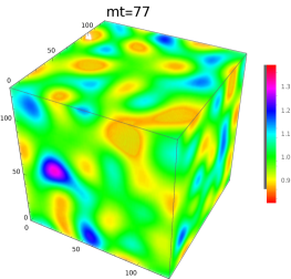
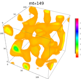
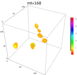
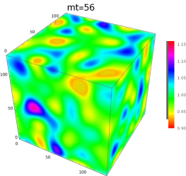
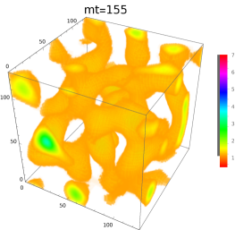
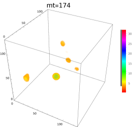
Figure 1: The panels show the fragmentation of AD condensate and the formation of Q-balls in the case of $K=0,\xi=10$ (upper panles) and $K=0.001,\xi=10$ (lower panels), respectively. The corresponding time scales are labeled in terms of $mt$ with $m\equiv m_{3/2}$. The input parameters are chosen as $m_{3/2}=100{\rm TeV}$, $\phi_{0}=10^{17}{\rm GeV}$, $\delta\phi/\phi_{0}=10^{-5}$, $dx=50dt,LH=0.5$. The average energy density is normalized to 1.

The initial small fluctuations of the AD condensate come dominantly from the primordial quantum fluctuations, which exited the horizon during inflation and re-entered the horizon afterwards. From the inflationary cosmology, it can be expected to be $|\delta\phi/\phi|\sim 10^{-5}$. The final amplitude of the gravity waves is proved to be independent of the size of the initial perturbation in the flat direction [24].

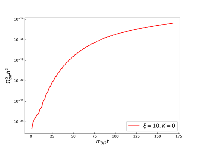
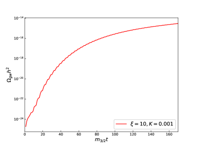
Figure 2: The panels show the temporal evolution of the present GW density parameter $\Omega_{gw}^{0}h^{2}$ for the two benchmarks points (in fig.1) with $K=0,\xi=10$ (left panel) and $K=0.001,\xi=10$ (right panel) , respectively.

We will discuss the Q-balls formation process and the emitted GWs with non-vanishing $\xi$, especially the most interesting $K\geq 0,\xi>0$ case. The numerical results for benchmark points $K=0,\xi=10$ and $K=0.001,\xi=10$ are shown in the panels of fig.1 and fig.2.

In the simulation of the two benchmark points, the gravitino mass $m_{3/2}$ in the scalar potential is chosen to be 100 TeV and the initial value of the homogeneous mode $\Phi_{0}$ is chosen to be $10^{17}{\rm GeV}$, which may correspond to the flat direction lifted by $n=9$. The AD condensate can fragment efficiently into Q-balls when the fluctuations produced by linear parametric resonance become significant and the dynamics become highly nonlinear. The process of the Q-balls formation can be seen in the panels of fig.1. From the panels, we can see the stages for AD fragmentation, the emerging of Q-balls and the further evolution of Q-balls, respectively. It is clear that Q-balls can be formed successfully in both cases.

The fragmentation process is not isotropic and non-spherical motions of the condensate can generate a quadrupole moment, which will emit GWs during Q-balls formation. The GWs are generated when the linear perturbation in the flat direction condensate starts growing. The corresponding GW productions associated with the fragmentation of AD field in the case $K=0$ and $K>0$ can reveal the information of evolution. The evolution of present GW density parameter as a function of the evolution time $m_{3/2}t$ are shown in fig.2 for the benchmark points $K=0,\xi=10$ and $K=0.001,\xi=10$, respectively.

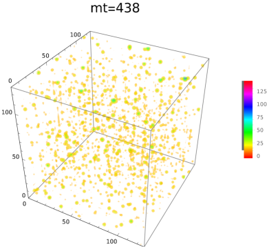
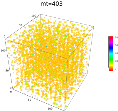
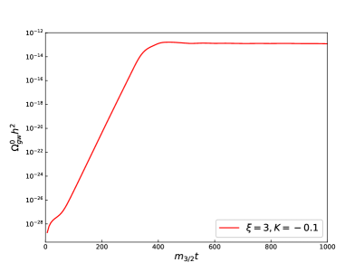
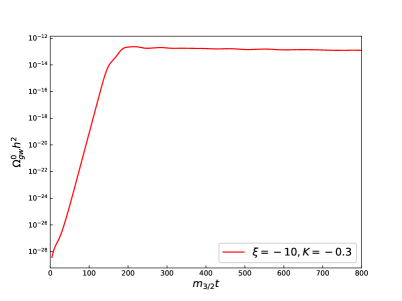
Figure 3: Benchmark points with $K=-0.1,\xi=3$ (left panels) and $K=-0.3,\xi=-10$ (right panels). The forms of the final-stage massive Q-balls for both cases are shown in the upper panels. The evolution of the GW density parameter $\Omega_{gw}^{0}h^{2}$ with respect to $m_{3/2}t$ are shown in the lower panels. The input parameters are chosen as $\phi_{0}=10^{16}{\rm GeV}$, $\delta\phi/\phi_{0}=10^{-5}$, $dx=50dt,LH=0.5$ with $m_{3/2}=100{\rm TeV}$.

The form of the final-stage massive Q-balls and the evolution of the present GW density parameter with negative $K$ and either sign of $\xi$ are also shown in fig.3. The setting of the input parameters are shown in the caption of this figure. We show the benchmark points $K=-0.1,\xi=3$ and $K=-0.3,\xi=-10$ in the left and right panels of fig.3, respectively. Although the value $K=-0.3$ is relatively large in case of $\xi=0$ without non-minimal gravitational couplings [24], it is still acceptable with the choice of negative value $\xi$, as discussed previously in subsection 3.1.

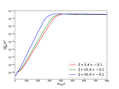
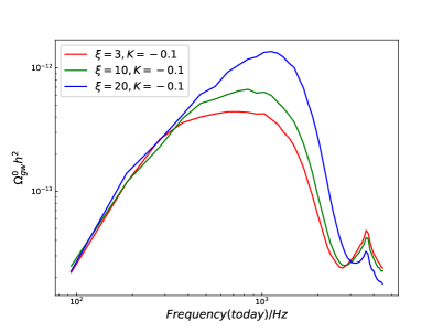
Figure 4: Same input parameters as fig.3. The evolution of the present GW density parameter $\Omega_{gw}^{0}h^{2}$ and its dependence on the choices of $\xi$ are shown in the left panel. The frequency bands of the GWs from Q-ball formation at the frequency ranging from $100$ Hz to $10^{3}$ Hz in each case are shown in the right panel.

The GW power spectrum for $K=-0.1$ with various value of $\xi$ are shown in fig.4. We can see that the final amplitude of the present GW density parameter $\Omega_{gw}^{0}h^{2}$ during the evolution is insensitive to the value of $\xi$. Different choices of $\xi$ lead to different growth rate of the GWs. The peak frequency $f_{P}$ of $\Omega_{gw}^{0}h^{2}$ is also insensitive to the choices of $\xi$ while the peak values of $\Omega_{gw}^{0}h^{2}$ depend on the choices of $\xi$. Larger $\xi$ will lead to larger peak value of $\Omega_{gw}^{0}h^{2}$. The peak frequency for GW power spectrum lies around a few KHz with our choice of $m_{3/2}=100{\rm TeV}$. Therefore, the stochastic GW backgrounds can not be observed by the current and upcoming interferometer based GW experiments. It was shown in [41] that the peak position of the GW power spectrum depends on the value of $m_{3/2}$. Larger values of $m_{3/2}$ lead to higher GW frequencies. Choosing a lower value of $m_{3/2}$ can shift the spectrum to lower frequency. However, we find that such a small-shifted GW power spectrum can still not be detected by the upcoming interferometer based GW experiments. As the gravitino mass is given by $m_{3/2}=F/\sqrt{3}M_{P}$, low SUSY breaking scale $F$ may cause low GW frequencies. If such stochastic GW signal are detected, it may give interesting information on the value of SUSY breaking scale.

We should note that our calculations ignore reheating and thermalization due to the AD condensate. Once the decay of the condensate is taken into account, the amplitude of the GWs will be attenuated. Such topics will be discussed in our subsequent studies. It is known that finite-temperature corrections to the flat direction potential can act as a source of SUSY breaking, which could have important effects on the dynamics of flat directions. Thermal corrections, whose exact effect depend on the temperature of the thermal bath $T$ and the nature of the AD condensate, can be important if the inflaton decays dominantly into the visible sector fields and produces MSSM degrees of freedom. In general, a precise calculation for the baryon asymmetry via the AD mechanism and GW productions should take them into account [42].

Simple treatment of thermal effects are based on the existence of a thermal plasma from inflaton decay at arbitrarily early times, which implicitly assumes that particles produced from decay of the inflaton immediately reach thermal equilibrium. In fact, assignment of a temperature $T$ to the reheat plasma is only justified after full thermal equilibrium is achieved. However, reheating and thermalization after inflation can be a very complicated process involving various perturbative and non-perturbative phenomena. For example, the helicity $\pm 3/2$ gravitino can be produced non-perturbatively from vacuum fluctuations after inflation [43]. Particles produced from inflaton decay typically have a non-thermal distribution, and the time scale of their equilibrium is model dependent. In a non-SUSY case, the inflaton usually decays via preheating unless its couplings to other fields are very small. The inflaton decay products thermalize very quickly because of the efficiency of interactions mediated by the massless gauge bosons of the SM. Therefore, the reheat temperature is mainly governed by the inflaton decay width. However, preheating is unlikely within supersymmetry because flat directions in the scalar potential are generically displaced towards a large VEV in the early Universe, which induce supersymmetry preserving masses to the inflaton decay products and consequently prohibit non-perturbative inflaton decay into MSSM fields [44]. Besies, the process of thermalization within SUSY is in general very slow [45, 46] because the VEV of the AD condensate can induces a large mass to the gauge fields via Higgs mechanism, thereby suppressing the rate of processes relevant for thermalization. If the entire SM gauge group is broken, thermalization can be delayed substantially. A full thermal equilibrium is generically established much later on when the VEV of the flat direction has substantially decreased. Therefore, Universe loiters in a phase of a quasi-thermal equilibrium after the decay of the inflaton, resulting in a very low reheat temperature, perhaps as low as O(TeV). The final reheat temperature depends on a thermalization time scale instead of the decay width of the inflaton.

4 Conclusions

We propose to introduce non-minimal couplings of Affleck-Dine (AD) field to gravity by adding the coupling of AD field to the Ricci scalar curvature. A possible realization to generate the $c_{0}|\Phi|^{2}R$ type coupling terms with a general $c_{0}$ in Jordan frame supergravity after SUSY breaking is given. The impacts of such non-minimal gravitational couplings for AD field is shown, especially on the Q-balls formation and the associated gravitational wave (GW) productions. New form of scalar potential for AD field in the Einstein frame is obtained. By numerical simulations, we find that, with non-minimal gravitational coupling to AD field, Q-balls can successfully form even with the choice of non-negative $K$ parameter for $\xi>0$. The associated GW productions as well as their dependences on the $\xi$ parameter are also discussed.

References

- [1] A. D. Sakharov, JETP Lett. 6, 24 (1967).
- [2] V. A. Kuzmin, V. A. Rubakov and M. E. Shaposhnikov, Phys. Lett. B 155, 36 (1985).
- [3] M. Fukugita and T. Yanagida, Phys. Lett. B 174, 45 (1986).
- [4] E.W. Kolb and M.S. Turner, The Early Universe, Adddison-Wesley, Reading, MA (1990).
-
[5]
I. Affleck and M. Dine, Nucl. Phys. B 249, 361 (1985);
- [6] Michael Dine, Alexander Kusenko, Rev. Mod. Phys. 76, 1 (2003) [arXiv:hep-ph/0303065 [hep-ph]].
- [7] Kari Enqvist, Anupam Mazumdar, Phys.Rept.380:99-234 (2003).
- [8] B. P. Abbott et al. (LIGO Scientific and Virgo Collaborations), Observation of Gravitational Waves from a Binary Black Hole Merger, Phys. Rev. Lett. 116, 061102 (2016).
- [9] C. Caprini et al., Science with the space-based interferometer eLISA. II: Gravitational waves from cosmological phase transitions, J. Cosmol. Astropart. Phys. 04 (2016)001.
- [10] K. Yagi and N. Seto, Detector configuration of DECIGO/BBO and identification of cosmological neutron-star binaries, Phys. Rev. D 83, 044011 (2011); Erratum, Phys. Rev. D 95, 109901 (2017).
- [11] A. Mazumdar and G. White, Rept. Prog. Phys. 82 (2019) no.7, 076901 doi:10.1088/1361-6633/ab1f55 [arXiv:1811.01948 [hep-ph]].
- [12] G. Rosen, J. Math. Phys. 9 (1968) 996; R. Friedberg, T. D. Lee and A. Sirlin, Phys. Rev. D 13, 2739 (1976); S. R. Coleman, Nucl. Phys. B 262, 263 (1985) [Erratum-ibid. B 269, 744 (1986)]; A. Kusenko, Phys. Lett. B 404, 285(1997).
-
[13]
T. Hiramatsu, M. Kawasaki and F. Takahashi, JCAP 1006, 008 (2010) [arXiv:1003.1779 [hep-ph]];
T. Multamaki and I. Vilja, Nucl. Phys. B 574, 130 (2000); T. Multamaki and I. Vilja, Phys. Lett. B 535, 170 (2002); T. Multamaki, Phys. Lett. B 511, 92 (2001); K. Enqvist, A. Jokinen, T. Multamaki and I. Vilja, Phys. Rev. D 63, 083501 (2001); E. Palti, P. M. Saffin and E. J. Copeland, Phys. Rev. D 70, 083520 (2004); M. I. Tsumagari, E. J. Copeland and P. M. Saffin, Phys. Rev. D78:065021(2008); L. Campanelli and M. Ruggieri, Phys. Rev. D 77, 043504 (2008). - [14] A. Kusenko, Phys. Lett. B 405, 108 (1997); A. Kusenko, M.E. Shaposhnikov, Phys. Lett. B 418, 46 (1998); S. Kasuya and M. Kawasaki, Phys. Rev. D 61, 041301 (2000).
- [15] K. Enqvist and J. McDonald, Phys. Lett. B 425, 309 (1998); S. Kasuya and M. Kawasaki, Phys. Rev. D 62, 023512 (2000).
- [16] S. Kasuya and M. Kawasaki, Phys. Rev. Lett. 85, 2677 (2000); S. Kasuya and M. Kawasaki, Phys. Rev. D 64, 123515 (2001).
-
[17]
K. Enqvist and J. McDonald, Phys. Lett. B 425, 309 (1998);
K. Enqvist and J. McDonald, Nucl. Phys. B538, 321 (1999);
F. Doddato and J. McDonald, JCAP 07, 004 (2013). - [18] Leszek Roszkowski, Osamu Seto, Phys. Rev. Lett. 98, 161304 (2007).
- [19] A. Kamada, M. Kawasaki and M. Yamada, Phys. Rev. D 91, no.8, 081301 (2015) doi:10.1103/PhysRevD.91.081301 [arXiv:1405.6577 [hep-ph]].
- [20] Fei Wang, Jin Min Yang, Nucl. Phys. B 709 (2005)409-418.
- [21] M. Dine, L. Randall and S. D. Thomas, Nucl. Phys. B 458, 291 (1996).
- [22] T. Gherghetta,C. Kolda and S.P. Martin, Nucl. Phys. B 468, 37 (1996).
- [23] A. Kusenko and A. Mazumdar, Phys. Rev. Lett. 101, 211301 (2008);
- [24] A. Kusenko, A. Mazumdar, and T. Multamaki, Phys. Rev. D 79, 124034 (2009);
- [25] Chiba, Takeshi and Kamada, Kohei and Yamaguchi, Masahide, Phys. Rev. D 81,8, 083503 (2010).
- [26] A. Mazumdar and J. Rocher, Phys. Rept. 497 (2011), 85-215 doi:10.1016/j.physrep.2010.08.001 [arXiv:1001.0993 [hep-ph]].
-
[27]
James M. Cline, Matteo Puel, Takashi Toma, Phys. Rev. D 101, 043014 (2020);
M. Kawasaki and S. Ueda, JCAP 04, 049 (2021). - [28] S. Ferrara, R. Kallosh, A. Linde, A. Marrani and A. Van Proeyen, Phys. Rev. D 82, 045003 (2010) [arXiv:1004.0712 [hep-th]].
- [29] H. M. Lee, JCAP 08, 003 (2010) [arXiv:1005.2735 [hep-ph]].
- [30] S. Ferrara, R. Kallosh, A. Linde, A. Marrani and A. Van Proeyen, Phys. Rev. D 83, 025008 (2011) [arXiv:1008.2942 [hep-th]].
- [31] S. V. Ketov and A. A. Starobinsky, Inflation and non-minimal scalar-curvature coupling in gravity and supergravity, JCAP 08 (2012) 022.
- [32] A.E. Nelson and N.J. Weiner, Extended anomaly mediation and new physics at 10-TeV, hep-ph/0210288.
- [33] K. Hsieh and M. A. Luty, JHEP 06, 062 (2007) [arXiv:hep-ph/0604256 [hep-ph]].
-
[34]
X. Du and F. Wang, NMSSM From Alternative Deflection in Generalized Deflected Anomaly
Mediated SUSY Breaking, Eur. Phys. J. C 78 (2018) 431 [arXiv:1710.06105];
F. Wang, Deflected anomaly mediated SUSY breaking scenario with general messenger-matter interactions, Phys. Lett. B 751 (2015) 402 [arXiv:1508.01299]. - [35] K. Enqvist and J. McDonald, Phys. Lett. B 425, 309 (1998); Nucl. Phys. B538, 321 (1999).
- [36] F. L. Bezrukov and M. Shaposhnikov, Phys. Lett. B 659, 703-706 (2008) doi:10.1016/j.physletb.2007.11.072 [arXiv:0710.3755 [hep-th]].
- [37] J. Garcia-Bellido, D. G. Figueroa and J. Rubio, Phys. Rev. D 79 (2009), 063531 doi:10.1103/PhysRevD.79.063531 [arXiv:0812.4624 [hep-ph]].
- [38] Juan Garcia-Bellido, Daniel G. Figueroa, and Alfonso Sastre, Phys. Rev. D 77, 043517.
- [39] Takeshi Chiba, Kohei Kamada, and Masahide Yamaguchi, Phys. Rev. D 81, 083503(2010).
- [40] Z. Huang, Phys. Rev. D 83, 123509 (2011).
- [41] Shuang-Yong Zhou, JCAP 1506 (2015)06,033.
- [42] R. Allahverdi and A. Mazumdar, New Journal of Physics 14 (2012) 125013.
- [43] A. L. Maroto and A. Mazumdar, Phys. Rev. Lett. 84 (2000), 1655-1658 doi:10.1103/PhysRevLett.84.1655 [arXiv:hep-ph/9904206 [hep-ph]].
- [44] R. Allahverdi and A. Mazumdar, Phys. Rev. D 76 (2007), 103526 doi:10.1103/PhysRevD.76.103526 [arXiv:hep-ph/0603244 [hep-ph]].
- [45] R. Allahverdi and A. Mazumdar, [arXiv:hep-ph/0505050 [hep-ph]].
- [46] R. Allahverdi and A. Mazumdar, JCAP 10 (2006), 008 doi:10.1088/1475-7516/2006/10/008 [arXiv:hep-ph/0512227 [hep-ph]].