Approximate Bayesian Computation of Bézier Simplices

Abstract

Bézier simplex fitting algorithms have been recently proposed to approximate the Pareto set/front of multi-objective continuous optimization problems. These new methods have shown to be successful at approximating various shapes of Pareto sets/fronts when sample points exactly lie on the Pareto set/front. However, if the sample points scatter away from the Pareto set/front, those methods often likely suffer from over-fitting. To overcome this issue, in this paper, we extend the Bézier simplex model to a probabilistic one and propose a new learning algorithm of it, which falls into the framework of approximate Bayesian computation (ABC) based on the Wasserstein distance. We also study the convergence property of the Wasserstein ABC algorithm. An extensive experimental evaluation on publicly available problem instances shows that the new algorithm converges on a finite sample. Moreover, it outperforms the deterministic fitting methods on noisy instances.

1 Introduction

Multi-objective optimization is a ubiquitous task in our life, which is the problem of minimizing multiple objective functions under certain constraints, denoted by

minimize $$\leavevmode\nobreak\ f(x):=(f_{1}(x),\dots,f_{M}(x))$$

subject to $$\leavevmode\nobreak\ x\in X(\subseteq\mathbb{R}^{N}).$$

Since the objective functions $f_{1},\dots,f_{M}:X\to\mathbb{R}$ are usually conflicting, we would like to consider their minimization according to the Pareto order defined as follows:

$$x\prec y\xLeftrightarrow{\mathrm{def}}\forall i\left[f_{i}(x)\leq f_{i}(y)\right]\land\exists j\left[f_{j}(x)<f_{j}(y)\right].$$

The goal is to find the Pareto set

$$X^{*}(f):=\Set{x\in X}{\forall y\in X\left[y\not\prec x\right]}$$

and the Pareto front

$$f(X^{*}(f)):=\Set{f(x)\in\mathbb{R}^{M}}{x\in X^{*}(f)}.$$

By solving the problem with numerical methods (e.g., goal programming [Miettinen, 1999, Eichfelder, 2008], evolutionary computation [Deb, 2001, Zhang and Li, 2007, Deb and Jain, 2014], homotopy methods [Hillermeier, 2001, Harada et al., 2007], Bayesian optimization [Hernandez-Lobato et al., 2016, Yang et al., 2019]), we obtain a finite set of points as an approximation of the Pareto set/front. In almost all cases, the dimensionality of the Pareto set and front is $M-1$ (see [Wan, 1977, 1978] for rigorous statement), which means that such a finite-point approximation suffers from the “curse of dimensionality”. As the number of objective functions $M$ increases, the number of points required to represent the entire Pareto set and front grows exponentially.

Fortunately, it is known that many problems have a simple structure of the Pareto set and front, which can be utilized to enhance approximation. Kobayashi et al. [2019] defined the simplicial problem whose Pareto set/front is homeomorphic to an $(M-1)$-dimensional simplex and each $(m-1)$-dimensional subsimplex corresponds to the Pareto set/front of an $m$-objective subproblem for all $1\leq m\leq M$ (see Figure 1). Hamada et al. [2020] showed that strongly convex problems are simplicial under mild conditions. They also showed that facility location [Kuhn, 1967] and phenotypic divergence modeling in evolutionary biology [Shoval et al., 2012] are simplicial. In airplane design [Mastroddi and Gemma, 2013] and hydrologic modeling [Vrugt et al., 2003], scatter plots of numerical solutions imply those problems are simplicial. Kobayashi et al. [2019] showed that the Pareto set and front of any simplicial problem can be approximated with arbitrary accuracy by a Bézier simplex.

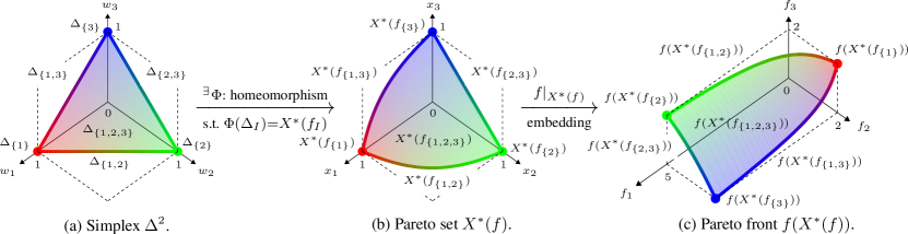
Figure 1: A simplicial problem $f=(f_{1},f_{2},f_{3}):\mathbb{R}^{3}\to\mathbb{R}^{3}$. An $M$-objective problem $f$ is simplicial if the following conditions are satisfied: (i) there exists a homeomorphism $\Phi:\Delta^{M-1}\to X^{*}(f)$ such that $\Phi(\Delta_{I})=X^{*}(f_{I})$ for all $I\subseteq\set{1,\dots,M}$; (ii) the restriction $f|_{X^{*}(f)}:X^{*}(f)\to\mathbb{R}^{M}$ is a topological embedding (and thus so is $f\circ\Phi:\Delta^{M-1}\to\mathbb{R}^{M}$).

A serious drawback of Bézier simplex fitting methods is the lack of robustness against noise. Kobayashi et al. [2019] assumed that the sample points lie exactly on the Pareto set/front. Tanaka et al. [2020] showed that introducing noise to the sample points drastically degrades the quality of approximation. Since multi-objective optimization often requires a great amount of computing resources, the outcome of numerical optimization methods may be rough, which is considered as a noisy sample from the Pareto set/front.

To make the fitting methods noise-resilient, in this paper, we extend the Bézier simplex model to a Bayesian one, propose an approximate Bayesian computation based on the Wasserstein distance, which we call WABC, and evaluate its asymptotic behavior. Our contributions are as follows:

• In Section 2, we propose an approximate Bayesian computation algorithm for Bézier simplex fitting (Algorithm 2), which is an extension of the deterministic fitting algorithm proposed in [Kobayashi et al., 2019].

• In Section 3, we analytically evaluate the bias of the WABC posterior (Theorem 3), and the acceptance rate of WABC (Theorem 4).

• In Section 4, we demonstrate the usefulness of the proposed method on noisy data sets.

2 Bézier Simplex Fitting

In this section, we review the definition of the Bézier simplex and some known regression algorithms. The existing methods, however, are basically deterministic algorithms and vulnerable to noise. To solve this problem, we propose a new Bayesian inference-based method.

2.1 Bézier simplex

Let us begin with the definition of the $(M-1)$-dimensional simplex,

$${\Delta^{{M}-1}}=\Set{{\bf t}=(t_{1},t_{2},\dots,t_{M})\in\mathbb{R}^{M}}{0\leq t_{m},\sum_{m=1}^{M}t_{m}=1}.$$

See Figure 1(a), which is $(M-1)=2$ case for example.

A Bézier simplex of order $D$ is defined as a polynomial map of $D$-degree from ${\Delta^{{M}-1}}$ to $\mathbb{R}^{M}$. To label each monomial, we introduce the set of degrees:

$$\mathbb{N}_{D}^{M}=\Set{{\bf d}=(d_{1},d_{2},\dots,d_{M})\in\mathbb{N}^{M}}{\sum_{m=1}^{M}d_{m}=D}.$$

In addition, we need to assign a vector ${{\bf p}_{{\bf d}}}\in\mathbb{R}^{M}$, which we call control point, to each degree ${\bf d}\in\mathbb{N}_{D}^{M}$. For a given set of control points $\{{{\bf p}_{{\bf d}}}\in\mathbb{R}^{M}\}_{{\bf d}\in\mathbb{N}_{D}^{M}}$, that we write it $\{{{\bf p}_{{\bf d}}}\}$ for short, the Bézier simplex is defined as

$${\bf b}_{\{{{\bf p}_{{\bf d}}}\}}({\bf t})=\sum_{{\bf d}\in\mathbb{N}_{D}^{M}}\begin{pmatrix}D\\ {\bf d}\end{pmatrix}t_{1}^{d_{1}}t_{2}^{d_{2}}\cdots t_{M}^{d_{M}}{{\bf p}_{{\bf d}}},$$

where ${\bf t}\in{\Delta^{{M}-1}}$, and $\begin{pmatrix}D\\ {\bf d}\end{pmatrix}$ is the multinomial coefficient.

2.2 Regression Model

From the definition, it is evident that Bézier simplices are continuous functions from ${\Delta^{{M}-1}}$ to the target space $\mathbb{R}^{M}$. Due to such a topological property, fitting the given data by a Bézier simplex works well if the data enjoyed the underlying simplex structure. The goal of the fitting is finding a set of control points $\{{{\bf p}_{{\bf d}}}\}$ that the corresponding Bézier simplex ${\bf b}_{\{{{\bf p}_{{\bf d}}}\}}$ reproduces data points, and there is some known prior work based on regression as follows.

The all-at-once fitting algorithm.

Kobayashi et al. [2019] proposed a Bézier simplex fitting algorithm: the all-at-once fitting. The all-at-once fitting requires a training set $\set{{\bf x}_{i}\in\mathbb{R}^{M}}{i=1,\dots,n}$ and aim to adjust all control points $\{{{\bf p}_{{\bf d}}}\}$ by minimizing the OLS loss: $\frac{1}{n}\sum_{i=1}^{n}\|{\bf x}_{i}-{\bf b}_{\{{{\bf p}_{{\bf d}}}\}}({\bf t}_{i})\|^{2}$, where ${\bf t}_{i}\leavevmode\nobreak\ (i=1,\dots,n)$ is a parameter corresponding to ${\bf x}_{i}$. Here, the parameter ${\bf t}_{i}$ for each ${\bf x}_{i}$ is unknown in advance. Thus, the all-at-once fitting repeats minimizing the OLS loss with respect to the parameters ${\bf t}_{i}\leavevmode\nobreak\ (i=1,\dots,n)$ and the control points $\{{{\bf p}_{{\bf d}}}\}$ alternatively.

The inductive-skeleton fitting algorithm.

Kobayashi et al. [2019] also propose a sophisticated method utilizing the simplex structure of the Bézier simplex: the inductive skeleton fitting. In this method, the authors recursively applied the all-at-once fitting to subsimplices of the Bézier simplex.

Drawbacks.

Both methods easily become unstable when fitting noisy samples. When their fitting algorithms minimize the OLS with respect to ${\bf t}_{i}\leavevmode\nobreak\ (i=1,\dots,n)$, the solution ${\bf t}_{i}$ is a foot of a perpendicular line from ${\bf x}_{i}$ to ${\bf b}_{\{{{\bf p}_{{\bf d}}}\}}(\Delta^{M-1})$. This calculation requires to solve nonlinear equations with Newton’s method, which is quite sensitive to noises included in ${\bf x}_{i}$ and also sometimes fails to converge.

2.3 Extension to Bayesian Model

To resolve the above problems, we propose a new fitting algorithm based on Bayesian inference. First of all, we describe the Bézier simplex model in a probabilistic manner.

Let $U_{\Delta^{{M}-1}}({\bf t})$ be the uniform distribution on the $(M-1)$-dimensional simplex ${\Delta^{{M}-1}}$. We define the likelihood of a point ${\bf x}$ as

$$p({\bf x}|\{{{\bf p}_{{\bf d}}}\})=\int_{{\Delta^{{M}-1}}}\delta_{{\bf x}-{\bf b}_{\{{{\bf p}_{{\bf d}}}\}}({\bf t})}U_{{\Delta^{{M}-1}}}({\bf t})d{\bf t},$$ (1)

where $\delta_{\bf x}$ is the Dirac distribution with mass on ${\bf x}$. Note that this conditional probability can be regarded as defining a generative model, which is the push-forward of the uniform distribution $U_{\Delta^{{M}-1}}({\bf t})$ by the Bézier simplex, i.e.

$${\bf y}\sim p(\cdot|\{{{\bf p}_{{\bf d}}}\})\Leftrightarrow{\bf t}\sim U_{\Delta^{{M}-1}}(\cdot),{\bf y}={\bf b}_{\{{{\bf p}_{{\bf d}}}\}}({\bf t}).$$ (2)

Bayesian inference.

To describe our Bayesian treatment of Bézier simplices, we focus on the general framework of Bayesian inference with parameter $\theta$ for the time being. In addition, we introduce a shorthand notation for the vector made of concatenating some vectors sharing the same dimension.

Definition 1 (aligned vector)

Suppose $\{{\bf x}_{i}\}_{i=1,2,\dots,n}$ is a set of $M$-dimensional vectors, we define the $(nM)$-dimensional vector,

$${\bf x}_{1:n} :=\begin{array}[]{ll}&[({\bf x}_{1})_{1},({\bf x}_{1})_{2},\dots,({\bf x}_{1})_{M},\\ &\ ({\bf x}_{2})_{1},({\bf x}_{2})_{2},\dots,({\bf x}_{2})_{M},\\ &\dots\\ &\ ({\bf x}_{n})_{1},({\bf x}_{n})_{2},\dots,({\bf x}_{n})_{M}],\end{array}=:[{\bf x}_{1}:{\bf x}_{2}:\cdots:{\bf x}_{n}],$$

by concatenating $\{{\bf x}_{i}\}_{i=1,2,\dots,n}$ in order of indexing, where $({\bf x}_{i})_{\mu}$ is the $\mu$-th component of the vector ${\bf x}_{i}$.

We use this notation to represent given data and synthetic data generated by models. For example, we denote the likelihood function of given data $\{{\bf x}_{i}\}_{i=1,2,\dots,n}$ as

$$p({\bf x}_{1:n}|\theta)=\prod_{i=1}^{n}p({\bf x}_{i}|\theta).$$ (3)

One of the main targets of Bayesian inference is the posterior distribution for $\theta$,

$$p_{\mathrm{posterior}}(\theta|{\bf x}_{1:n})=\frac{p({\bf x}_{1:n}|\theta)p_{\mathrm{prior}}(\theta)}{p({\bf x}_{1:n})},$$ (4)

where $p_{\mathrm{prior}}(\theta)$ is a certain prior distribution, and $p({\bf x}_{1:n})$ is the marginal distribution. Once we got the explicit form of the posterior, we can directly treat the model in probabilistic way based on it. However, this is not always possible. In fact, we cannot write down the explicit form of our likelihood function (1), neither the posterior in that case.

Approximate Bayesian Computation.

So we need an alternative way. In the present paper, we use the approximate Bayesian computation (ABC), which is an approximated sampling method from the posterior, defined in Algorithm 1. To execute the algorithm, we only need to know how to sample from the model distribution.

Algorithm 1 $\{\theta_{i}\}_{i=1,2,\dots,N_{\mathrm{ABC}}}\sim p_{\mathrm{ABC}}^{(\delta)}(\theta|{\bf x}_{1:n})$

0:  threshold $\delta$, number of samples $N_{\mathrm{ABC}}$, data ${\bf x}_{1:n}$, distance $d$

  $\theta_{\mathrm{accepted}}=\phi$

  while length$(\theta_{\mathrm{accepted}})<N_{\mathrm{ABC}}$ do

     draw parameter from the prior: $\theta\sim p_{\mathrm{prior}}(\theta)$

     draw ${\bf y}_{1:m}=[{\bf y}_{1}:{\bf y}_{2}:\dots:{\bf y}_{m}]$ for ${\bf y}_{j}\sim p({\bf y}|\theta)$ (i.i.d.)

     if $d({\bf x}_{1:n},{\bf y}_{1:m})\leq\delta$ then

        $\theta_{\mathrm{accepted}}=\theta_{\mathrm{accepted}}\cup\{\theta\}$

     end if

  end while

  return  $\theta_{\mathrm{accepted}}$

We can formally write down the probability distribution for $\theta$ that corresponds to the above sampling algorithm as

$$p_{\mathrm{ABC}}^{(\delta)}(\theta|{\bf x}_{1:n})=\frac{\int_{d({\bf x}_{1:n},{\bf y}_{1:m})\leq\delta}p({\bf y}_{1:n}|\theta)p_{\mathrm{prior}}(\theta)d{\bf y}_{1:m}}{p_{\mathrm{ABC}}^{(\delta)}({\bf x}_{1:n})},$$ (5)

where $d({\bf x}_{1:n},{\bf y}_{1:m})$ is a certain distance function that characterizes the algorithm itself, and $p_{\mathrm{ABC}}^{(\delta)}({\bf x}_{1:n})$ is the normalization factor.

The choice of the distance function strongly influences the performance of the algorithm. In the literature [Barber et al., 2015, Robert, 2016], it is common to introduce a certain $q$-dimensional summary statistics ${\bf s}_{{\bf x}}=T({\bf x}_{1:n})$, ${\bf s}_{{\bf y}}=T({\bf y}_{1:m})$, and define the distance function as $d({\bf x}_{1:n},{\bf y}_{1:m}):=d_{\mathrm{E}}({\bf s}_{{\bf x}},{\bf s}_{{\bf y}})$ by using the Euclidean distance:

$$d_{\mathrm{E}}({\bf a},{\bf b})=\sqrt{\sum_{\mu=1}^{q}|({\bf a})_{\mu}-({\bf b})_{\mu}|^{2}}.$$ (6)

In such a case, there is a known result on the bias of the expected value for an arbitrary function of $\theta$ calculated by ABC.

Theorem 1 (Barber et al. [2015])

Let $h(\theta)$ be a function of $\theta$ that $\mathbb{E}_{\mathrm{posterior}}[h(\theta)]$ is not divergent. If the summary statistics $T$ is sufficient and the likelihood is three times continuously differentiable with respect to ${\bf s}_{\bf x}=T({\bf x}_{1:n})$, then the following equality holds for ABC defined by the Euclidean distance:

$$\mathbb{E}_{\mathrm{ABC}}[h(\theta)]=\mathbb{E}_{\mathrm{posterior}}[h(\theta)]+C_{h}({\bf s}_{\bf x})\delta^{2}+\mathcal{O}(\delta^{3}),$$

where $C_{h}({\bf s}_{\bf x})$ is a value depending only on ${\bf s}_{\bf x}$ and the function $h$.

The bias term always scales as $\delta^{2}$, and it means that the ABC sampling based on the statistics $T$ and the Euclidean distance is unbiased by taking limit $\delta\to 0$. It sounds good, however, there is a complementary theorem on the acceptance of the ABC procedure. To illustrate it, we introduce the definition of the Euclidean ball:

Definition 2 (Euclidean Ball)

We define the $q$-dimensional Euclidean ball with radius $\delta$ and center ${\bf x}$ as follows,

$$B_{\delta}^{q}({\bf x})=\Set{{\bf y}\in\mathbb{R}^{q}}{d_{\mathrm{E}}({\bf x},{\bf y})\leq\delta},$$

where $d_{\mathrm{E}}(\cdot,\cdot)$ is the Euclidean distance defined in (6). In addition to it, we denote its ${\bf x}$-independent volume as $|B_{\delta}^{q}({\bf x})|=|B_{\delta}^{q}|$.

Here, we know the following explicit form:

$$|B_{\delta}^{q}|=\frac{\pi^{q/2}}{\Gamma(\frac{q}{2}+1)}\delta^{q},$$ (7)

where $\Gamma$ is the Gamma function. So it scales as $\delta^{q}$, and this fact is useful to draw out the meaning of the following theorem on the acceptance probability of the ABC procedure.

Theorem 2 (Barber et al. [2015])

If the summary statistics $T$ is sufficient and the likelihood is three times continuously differentiable with respect to ${\bf s}_{\bf x}=T({\bf x}_{1:n})$, then the acceptance probability of ABC defined by the Euclidean distance is

$$p_{\mathrm{accept}}=p({\bf s}_{\bf x})|B_{\delta}^{q}|(1+o(1)),$$

and we need to run $N_{\mathrm{ABC}}/p_{\mathrm{accept}}$ accept/reject trials during Algorithm 1 in average for gathering $N_{\mathrm{ABC}}$ samples.

Combining to the scale $\delta^{q}$ in the volume $|B_{\delta}^{q}|$, it means that the computational complexity explodes when $\delta\to 0$. One remedy for it is to adjust the prior $p_{\mathrm{prior}}(\theta)$ so that $p({\bf s}_{\bf x})=\int p({\bf s}_{\bf x}|\theta)p_{\mathrm{prior}}(\theta)d\theta$ takes relatively large value, and that is our strategy for Bayesian Bézier simplex model.

ABC of Bézier simplices.

Now, let us come back to the Bézier simplex model: $\theta=\{{{\bf p}_{{\bf d}}}\}$, and likelihood defined in (1) tentatively. On the prior $p_{\mathrm{prior}}(\{{{\bf p}_{{\bf d}}}\})$, we take it as follows:

$$p_{\mathrm{prior}}(\{{{\bf p}_{{\bf d}}}\})=\prod_{{\bf d}\in\mathbb{N}_{D}^{M}}p({{\bf p}_{{\bf d}}}|{\bf m}_{\bf d},\Sigma_{\bf d}),$$ (8)

where $p({\bf p}|{\bf m},\Sigma)$ is the multivariate normal distribution with hyper parameters, mean vector ${\bf m}$ and covariance matrix $\Sigma$.

If the likelihood were also defined by a certain multivariate normal distribution, then the prior (8) is conjugate prior. In such a case, Bayesian updates of the posterior can be reduced to updates of hyperparameters, $\{{\bf m}_{\bf d},\Sigma_{\bf d}\}$.

It is not clear whether our likelihood (1) defined by Bézier simplices is conjugate to the prior (8), however, we apply the updates of $\{{\bf m}_{\bf d},\Sigma_{\bf d}\}$ calculated by ABC samples. It may sound out of theory a little, but we would like to emphasize that:

1. If there is just one peak, the posterior is well approximated by the multivariate normal distribution around the peak.

2. We can discard the description of the “posterior updates,” and consider successive Bayesian inference just by changing its prior.

Algorithm 2 ABC of Bézier simplex

0:  data ${\bf x}_{1:n}$, degree of Bézier simplex $D$, positive integers $N_{\mathrm{updates}},N_{\mathrm{ABC}},N_{\delta}$, initial $\{{\bf m}_{\bf d},\Sigma_{\bf d}\}$ and $\delta>0$

  for $n_{\mathrm{trial}}$ in range($N_{\mathrm{updates}}$) do

     set the prior as $p_{\mathrm{prior}}(\{{{\bf p}_{{\bf d}}}\})=p(\{{{\bf p}_{{\bf d}}}\}|\{{\bf m}_{\bf d},\Sigma_{\bf d}\})$

     draw control points: $\{{{\bf p}_{{\bf d}}}\}_{1:N_{\mathrm{ABC}}}\sim p_{\mathrm{ABC}}^{(\delta)}(\{{{\bf p}_{{\bf d}}}\}|{\bf x}_{1:n})$

     $\{{\bf m}_{\bf d},\Sigma_{\bf d}\}\leftarrow\{\text{mean}(({{\bf p}_{{\bf d}}})_{1:N_{\mathrm{ABC}}})$, $\text{cov}(({{\bf p}_{{\bf d}}})_{1:N_{\mathrm{ABC}}})\}$

     update $\delta$ as follows

      calculate ”mean $d$ between model and data”

       $\{{{\bf p}_{{\bf d}}}\}_{1:N_{\delta}}\sim p(\{{{\bf p}_{{\bf d}}}\}|\{{\bf m}_{\bf d},\Sigma_{\bf d}\})$

       $({\bf y}_{1:n})_{1:N_{\delta}}\sim p(\cdot|\{{{\bf p}_{{\bf d}}}\}_{1:N_{\delta}})$

       $\epsilon=\frac{1}{N_{\delta}}\sum_{\alpha=1}^{N_{\delta}}d({\bf x}_{1:n},({\bf y}_{1:n})_{\alpha})$

      update $\delta$

       $\delta=0.9\epsilon$

  end for

  return  $\{{\bf m}_{\bf d},\Sigma_{\bf d}\}$

In addition, it would be better to take smaller $\delta$ because of Theorem 1. To do so, we apply an adaptive update of $\delta$ also. We describe our algorithm for the Bézier simplex model in Algorithm 2.

3 Wasserstein ABC and its Convergence Properties

The next issue on applying ABC to Bézier simplex is the choice of the summary statistics $T$ and the distance function $d$ in defining ABC posterior (5). Our likelihood (1) is slightly complicated, and it seems to be difficult to get any good (dimensionally reduced) sufficient statistics as Theorem 1 and Theorem 2 assumed.

There is, however, a trivial sufficient statistics, $T=\mathrm{id}$. In this case, we can employ the usual the Euclidean distance to measure two point clouds: $d({\bf x}_{1:n},{\bf y}_{1:n})=d_{\mathrm{E}}({\bf x}_{1:n},{\bf y}_{1:n})$ by concatenating ${\bf x}_{i}$ and ${\bf y}_{i}$ into $q=nM$-dimensional vectors as defined in Definition 1. In this case, we can guarantee the convergence and estimate its bias by utilizing Theorem 1.

However, such implementation is not practical because of too low acceptance probability. If we apply Theorem 2 by substituting $q=nM$, then, the denominator scales $(nM)!!$ approximately, and it means that the almost samples will be rejected if the number of samples $n$ increased.

So we take another better choice using Wasserstein distance, and we call the resultant ABC algorithm as WABC algorithm. In the later experiments, we use the 2-Wasserstein distance to measure the distance between the data ${\bf x}_{1:n}$ and the model samples ${\bf y}_{1:m}$. In addition, we take $m=n$ for simplicity. In such case, the definition of the 2-Wasserstein distance reduces to the following form:

$$d_{\mathrm{W}}({\bf x}_{1:n},{\bf y}_{1:n})=\sqrt{\min_{\sigma\in S_{n}}\frac{1}{n}\sum_{i=1}^{n}d_{\mathrm{E}}({\bf x}_{i},{\bf y}_{\sigma(i)})^{2}},$$ (9)

where $\sigma\in S_{n}$ runs for permutation of $n$ indices.

In this case, there is also a known work proving its convergence at $\delta\to 0$ [Bernton et al., 2019]. In practical use, however, it would be important to know how the expected value based on WABC with nonzero $\delta$ differs from the expected value for the true posterior.

We can prove that the bias between WABC posterior and the true posterior also scales as $\delta^{2}$ like Theorem 1. This is one of the main theorems of the present paper:

Theorem 3

Let $h(\theta)$ be a function of $\theta$ that $\mathbb{E}_{\mathrm{posterior}}[h(\theta)]$ is not divergent, and the likelihood is three times continuously differentiable with respect to ${\bf x}_{1:n}$, then WABC also has order $\delta^{2}$ bias:

$$\mathbb{E}_{\mathrm{WABC}}[h(\theta)]=\mathbb{E}_{\mathrm{posterior}}[h(\theta)]+C_{h}({\bf x}_{1:n})\delta^{2}+\mathcal{O}(\delta^{3}),$$

where $C_{h}({\bf x}_{1:n})$ is a value depending only on ${\bf x}_{1:n}$ and the function $h$.

We give its proof in the Appendix. Here, instead, we show some empirical results with simpler models here. In the first case (a), we define our Bayesian model as

$$p_{\mathrm{prior}}=N(0,1),\quad p(\cdot|\theta)=N(\theta,1),$$

and one-dimensional data $x_{1:n}$ generated by $p_{\mathrm{data}}=N(-1.5,1)$. As well known, prior $N(0,1)$ is a conjugate prior for $N(\theta,1)$, and we can easily get the corresponding posterior, which gives

$$\mathbb{E}_{\mathrm{posterior}}[\theta]=\frac{\sum_{i=1}^{n}x_{i}}{n+1}.$$

In the next setup (b), we define our Bayesian model as

$$p_{\mathrm{prior}}=N(0,1),\quad p(\cdot|\theta)=\begin{cases}U(0,\theta)&(\theta>0)\\ U(\theta,0)&(\theta<0)\end{cases},$$

and data $x_{1:n}$ generated by $p_{\mathrm{data}}=U(0,1),$ where $U(a,b)$ is the uniform distribution. In this case, the posterior is slightly non-trivial, but we can calculate the expectation of $\theta$ as

$$\mathbb{E}_{\mathrm{posterior}}[\theta]=\frac{\int_{1}^{\infty}\frac{e^{-\frac{\theta^{2}}{2}}}{|\theta|^{n-1}}d\theta}{\int_{1}^{\infty}\frac{e^{-\frac{\tilde{\theta}^{2}}{2}}}{|\tilde{\theta}|^{n}}d\tilde{\theta}},$$

which we assume $\max\{x_{i}\}=1$ for simplicity.

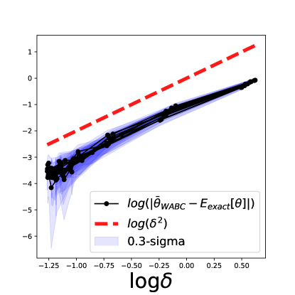
(a) Case 1: Gaussian

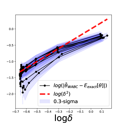
(b) Case2: Uniform

Figure 2: Numerical experiments to check Theorem 3. Horizontal axis is $log\delta$, vertical axis is $\log|\bar{\theta}_{\mathrm{WABC}}-\mathbb{E}_{\mathrm{posterior}}[\theta]|$ for black/blue plot, and $\log\delta^{2}$ (prediction by Theorem 3) for red line. Their coefficients seem to be identical near $\delta\approx 0$.

In Figure 2, we plot $\log|\bar{\theta}_{\mathrm{WABC}}-\mathbb{E}_{\mathrm{posterior}}[\theta]|$ on the vertical axis and $\log\delta$ on the horizontal axis with 10 trials with datasize $n=100$. $\bar{\theta}_{\mathrm{WABC}}$ is the empirical value of $\mathbb{E}_{\mathrm{WABC}}[\theta]$ defined as

$$\bar{\theta}_{\mathrm{WABC}}=\frac{1}{N_{\mathrm{ABC}}}\sum_{i=1}^{N_{\mathrm{ABC}}}(\theta_{\mathrm{accepted}})_{i}.$$

We compute it with $N_{\mathrm{ABC}}=1000$ by Algorithm 1 based on the Wasserstein distance (9).

In addition, we perform a linear regression $\log|\bar{\theta}_{\mathrm{WABC}}-\mathbb{E}_{\mathrm{posterior}}[\theta]|\approx c_{1}\log\delta+c_{0}$ for each trial and calculate the mean and std of the coefficient $c_{1}$:

$$\begin{array}[]{c|cc}&\text{$c_{1}$(fitted by all points)}&\text{$c_{1}$(fitted by middle points)}\\ \hline\cr\text{(a)}&1.98\pm 0.05&2.13\pm 0.16\\ \text{(b)}&1.65\pm 0.21&2.08\pm 0.33\end{array}$$

All results show $c_{1}\approx 2$ and support Theorem 3, i.e. the $\delta^{2}$ scaling in both cases. As the final theoretical result, let us show a scale of acceptance probability in WABC.

Theorem 4

If the likelihood is three times continuously differentiable with respect to ${\bf x}_{1:n}$, then the acceptance probability of WABC is

$$p_{\mathrm{accept}}=(n!)p({\bf x}_{1:n})|B_{\sqrt{n}\delta}^{q}|(1+o(1))$$

where $q=nM$. We need to run $N_{\mathrm{ABC}}/p_{\mathrm{accept}}$ accept/reject trials during Algorithm 1 in average for gathering $N_{\mathrm{ABC}}$ samples.

We give the proof of Theorem 4 in the Appendix. Compared to Theorem 2 by using $T=\mathrm{id}$, the acceptance probability is increased by $(n!)$ scale in numerator that cancels $1/(nM)!!$ in $|B_{\sqrt{n}\delta}^{q}|$, and it means the acceptance is drastically improved.

Remark

We restrict ourselves within the 2-Wasserstein distance that makes proof a little simple, however, the scaling laws with respect to $\delta$ in Theorem 3 and Theorem 4 seem to be valid even if we take the $p$-Wasserstein distance to define WABC.

4 Experiments

Now, we turn to the ABC for Bézier simplex fitting. In this section, we examine performances of our proposed method based on the 2-Wasserstein distance for Bézier simplex fitting using Pareto front samples.

4.1 Experimental settings

Data Sets

In the numerical experiments, we employed four synthetic problems with known Pareto fronts, all of which are simplicial problems. Schaffer is a two-objective problem, whose Pareto front is a curved line that can be triangulated into two vertices and one edge. 3-MED and Viennet2 are three objective problems. Their Pareto fronts are a curved triangle that can be triangulated into three vertices, three edges and one face. 5-MED is a five-objective problem. Its Pareto front is a curved pentachoron. We generated Pareto front samples of 3-MED and 5-MED by AWA(objective) using default hyper-parameters [Hamada et al., 2010]. Pareto front samples of the other problems were taken from jMetal 5.2. The formulation and data description of each problem are shown in the Appendix.

Settings

To assess the robustness of the proposed method, we consider the fitting problem with training points including the Gaussian noise. For a given dataset, we randomly choose $n$ points $\{{\bf x}_{i}\}_{i=1,2,\ldots,n}$ as a training dataset. Then, we consider fitting a Bézier simplex ${\bf b}({\bf t})\leavevmode\nobreak\ ({\bf t}\in\Delta^{M-1})$ to the set $\{\tilde{{\bf x}}_{i}\}_{i=1,2,\ldots,n}$, where $\tilde{{\bf x}}_{i}={\bf x}_{i}+\varepsilon_{i}\leavevmode\nobreak\ (\varepsilon_{i}\sim N(\boldsymbol{0},\sigma{\bf I})).$ Also, we use the set $\{{\bf x}_{i}\}_{i=1,2,\ldots,n}$ as a validation dataset not including the Gaussian noise. For each dataset, experiments were conducted on all combinations of the sample size $n\in\{50,100,150\}$ and the noise scale $\sigma\in\{0,0.05,0.1\}$.

In this experiment, we estimated the Bézier simplex with degree $D=3$, and compared the following two methods:

All-at-once

the all-at-once fitting [Kobayashi et al., 2019],

WABC

our proposed ABC algorithm (Algorithm 2) based on the 2-Wasserstein distance.

Here, we omitted the inductive skeleton fitting [Kobayashi et al., 2019] from our comparison because it requires a stratified subsample from skeletons of a simplex and such subsample is not included in each dataset we used. For WABC, we set the maximum number of update $N_{\mathrm{update}}=50$ and $N_{\delta}=100$. In addition, we set the initial ${\bf m}_{{\bf d}}$ as the vertices of the Beźier simplex, to be the single objective optima, and the rest of the control points were set to be the simplex grid spanned by them. The initial $\Sigma_{{\bf d}}$ was set to $0.1\times{\bf I}$. With the initial $\{{\bf m}_{{\bf d}},\Sigma_{{\bf d}}\}$, we set initial $\delta$ as the mean of the Wasserstein distances:

$$\delta=\frac{1}{N_{\delta}}\sum_{\alpha=1}^{N_{\delta}}d_{\mathrm{W}}(\tilde{{\bf x}}_{1:n},({\bf y}_{1:n})_{\alpha}),$$

where $\{{{\bf p}_{{\bf d}}}\}_{1:N_{\delta}}\sim p(\{{{\bf p}_{{\bf d}}}\}|\{{\bf m}_{{\bf d}},\Sigma_{{\bf d}}\})$ and $({\bf y})_{1:N_{\delta}}\sim p(\cdot|\{{{\bf p}_{{\bf d}}}\}_{1:N_{\delta})}$. We terminated WABC (Algorithm 2) when the number of accepted $\theta=\{{{\bf p}_{{\bf d}}}\}$ did not reach $N_{\delta}$ after it generated $10^{5}$ sets of control points, or when the updated $\Sigma_{{\bf d}}$ satisfied the following condition:

$$\max_{{\bf d}\in\mathbb{N}_{D}^{M}}\lambda_{\max}(\Sigma_{{\bf d}})\leq 10^{-5},$$

where $\lambda_{\max}(\Sigma_{{\bf d}})$ is the maximum eigenvalue of $\Sigma_{{\bf d}}$.

Performance Measures

To evaluate the approximation quality of estimated hyper-surfaces, we used the generational distance (GD) [Van Veldhuizen, 1999] and the inverted generational distance (IGD) [Zitzler et al., 2003]:

$$\textrm{GD}(X,Y)\coloneqq\frac{1}{|X|}\sum_{x\in X}\min_{y\in Y}\|x-y\|,$$

$$\textrm{IGD}(X,Y)\coloneqq\frac{1}{|Y|}\sum_{y\in Y}\min_{x\in X}\|x-y\|,$$

where $X$ is a finite set of points sampled from an estimated hyper-surface and Y is a validation set. Roughly speaking, GD and IGD assess precision and recall of the estimated Bézier simplex, respectively. That is, when the estimated front has a false positive area that is far from the Pareto front, GD gets high. Conversely, when the Pareto front has a false negative area that is not covered by the estimated front, IGD gets high. Thus, we can say that the estimated hyper-surface is close to the Pareto front if and only if both GD and IGD are small. When we calculate GD and IGD for the all-at-once fitting and WABC, we randomly generated $1000$ parameters $\{{\bf t}_{i}\}_{i=1,2,\ldots,1000}$ from the uniform distribution $U_{\Delta^{{M}-1}}(\cdot)$ and set $X=\{{\bf b}({\bf t}_{i})\}_{i=1,2,\ldots,1000}$ as a set of sampled points on the estimated Bézier simplex. For each dataset and $(n,\sigma)$, we repeated experiments 20 times with different training sets and computed the average and the standard deviations of their GDs and IGDs.

All methods were implemented in Python 3.7.1 and run on Ubuntu 18.04 with an Intel Xeon CPU E5-2640 v4 (2.40GHz) and 128 GB RAM. When we calculated the Wasserstein distance, we solved a linear optimization problem with POT package [Flamary and Courty, 2017].

4.2 Results

Table 1 shows the average and the standard deviation of the computation time, GD and IGD when $n=100$ and $\sigma\in\{0,0.05,0.1\}$. The results with $n=50$ and 150 are provided in the supplementary materials (see Table 3 and Table 4). In Table 1, we highlighted the best score of GD and IGD out of the all-at-once fitting and WABC where the difference is at a significant with significant level $p=0.05$ by the Wilcoxon rank-sum test.

First, let us focus on the results of $M=2$, Schaffer. In the case of Schaffer, we can observe that while the all-at-once fitting achieved lower GD and IGD than that of WABC when $\sigma=0$, WABC outperformed the all-at-once fitting in GD when $\sigma=0.1$. Next, we focus on the results of $M\geq 3$. From the results of $M\geq 3$ shown in Table 1, we can see that WABC consistently outperformed the all-at-once fitting in both GD and IGD. Especially in 5-MED with $\sigma=0.1$, the average GD and IGD of the all-at-once fitting 0.449 and 0.474, respectively, each of which is more than three times larger than that of WABC. For computational time, Table 1 shows that WABC is generally slower than the all-at-once fitting especially with large $M$. In the case of 5-MED with $\sigma=0.0$ for example, the average computational time of WABC is about 3000 seconds, which is more than 100 times longer than that of the all-at-once method. For the results with $n=50$ and 150, we can observe the similar tendencies as described above (see Tables 3 and 4).

Table 1: GD and IGD (avg.$\pm$s.d. over 20 trials) with $n=100$. The best scores with significance level $p<0.05$ are shown in bold.

Problem	$\sigma$		WABC			All-at-once
		Time	GD	IGD	Time	GD	IGD
Schaffer	0	53.4	8.92E-03$\pm$2.66E-03	9.39E-03$\pm$3.06E-03	2.8	2.52E-03$\pm$3.37E-05	1.29E-03$\pm$3.77E-04
($M=2$)	0.05	220.1	1.12E-02$\pm$3.20E-03	1.09E-02$\pm$3.50E-03	2.0	1.25E-02$\pm$4.37E-03	1.70E-02$\pm$8.67E-03
	0.1	443.6	1.82E-02$\pm$7.56E-03	1.84E-02$\pm$9.20E-03	2.4	2.79E-02$\pm$1.22E-02	2.28E-02$\pm$9.03E-03
3-MED	0	660.1	5.02E-02$\pm$2.10E-03	3.36E-02$\pm$2.39E-03	3.4	1.05E-01$\pm$9.28E-03	4.21E-02$\pm$2.22E-03
($M=3$)	0.05	1130.7	5.71E-02$\pm$3.01E-03	3.93E-02$\pm$4.03E-03	3.0	1.09E-01$\pm$1.10E-02	5.06E-02$\pm$8.49E-03
	0.1	805.1	7.99E-02$\pm$6.05E-03	5.24E-02$\pm$6.45E-03	3.9	1.29E-01$\pm$2.09E-02	6.95E-02$\pm$2.15E-02
Viennet2	0	386.3	2.09E-02$\pm$4.43E-03	2.57E-02$\pm$3.18E-03	10.2	9.29E+00$\pm$1.29E+01	9.28E-02$\pm$4.64E-02
($M=3$)	0.05	1196.7	4.47E-02$\pm$4.24E-03	3.39E-02$\pm$5.11E-03	4.2	1.04E-01$\pm$5.76E-02	6.81E-02$\pm$2.16E-02
	0.1	1113.9	9.50E-02$\pm$1.38E-02	6.00E-02$\pm$1.46E-02	6.3	1.11E-01$\pm$1.83E-02	1.14E-01$\pm$3.42E-02
5-MED	0	3083.0	8.82E-02$\pm$6.77E-03	1.28E-01$\pm$1.31E-02	29.0	1.53E-01$\pm$2.42E-02	1.95E-01$\pm$1.23E-02
($M=5$)	0.05	2292.1	9.83E-02$\pm$7.70E-03	1.36E-01$\pm$1.15E-02	31.8	1.82E-01$\pm$4.59E-02	2.02E-01$\pm$2.23E-02
	0.1	1846.0	1.24E-01$\pm$9.70E-03	1.55E-01$\pm$1.05E-02	79.3	4.49E-01$\pm$7.30E-01	4.74E-01$\pm$8.50E-01

4.3 Discussion

In this section, we discuss the results of our numerical experiments and the practicality of our WABC.

Approximation accuracy

For each problem instance $M\geq 3$, WABC consistently achieved better GD and IGD. While WABC adjusts control points with the Bayesian estimation, the all-at-once fitting is a point estimation. Thus, the number of control points to be estimated increases for large $M$ and the all-at-once fitting seems to be over-fitted to the training data when the number of training points is small. This is the reason why IGDs given the all-at-once method were worse than those of our WABC with large $M$.

Next, we discuss the results of GD. Figure 3 and Figure 4 depict points on the training dataset, the estimated Bézier simplex, and the Pareto-front from the 3-MED with $\sigma=0$ and 0.1, respectively. From these figures, we first observe that the Bézier simplex estimated by the all-at-once fitting was overly spreading and the one obtained by WABC was not. The all-at-once fitting only considers the distance from each training point to the Bézier simplex, which does no impose that all points on the Bézier simplex are close to the training points. On the other hand, WABC minimizes the Wasserstein distance between the set of data points and the one on the Bézier simplex. Thus, WABC can avoid the issue of over-spreading of the estimated Bézier simplex, which is the reason why WABC achieved better GDs.

Robustness

Next, we discuss the robustness of WABC and the all-at-once fitting. As we described in the results part, WABC obtained better GDs and IGDs than the all-at-once fitting even when $\sigma$ is large. Also, comparing Figure 3 with Figure 4, we can see that the shape of the Bézier simplex estimated by the all-at-once fitting was changed when the training points include noise. On the other hand, the shape of the Bézier simplex obtained by WABC with $\sigma=0,0.1$ is not so different from each other.

The all-at-once fitting calculates the distance between each training point and the Bézier simplex by drawing perpendicular lines from the data points to the simplex, which is quite sensitive to the perturbation of training points. Whereas, WABC does not require such calculation because it minimizes the Wasserstein distance, which contributes to its robustness against noise.

(a) WABC

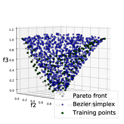
(b) All-at-once

Figure 3: Bézier triangles for 3-MED with $\sigma=0$.

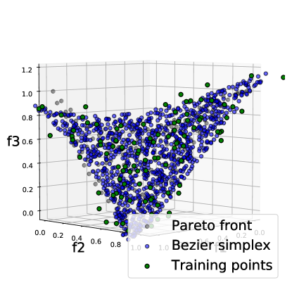
(a) WABC

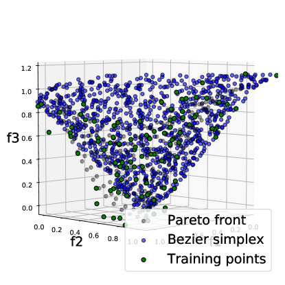
(b) All-at-once

Figure 4: Bézier triangles for 3-MED with $\sigma=0.1$.

Computation time

For computation time, we have to point out that WABC was certainly slower than the all-at-once method especially when $M$ was large. As we have shown in the previous section, the acceptance rate decreases in WABC if $M$ increases. In addition, WABC evaluates the Wasserstein distance, which requires to solve a linear optimization problem. For these reasons, WABC is expected to be slower than the all-at-once method.

In the context of practical use cases of multi-objective optimization, however, we believe that this issue does not affect the practicality of WABC so much and can be alleviated. First, for multi-objective optimization problems in the real world, the number of objective functions $M$ is usually less than 10 and at most 15 (Li et al. [2015], von Lücken et al. [2014]). Secondly, many real-world problems involve expensive simulations and/or experiments to evaluate solutions and the available sample size is often limited. In these situations, the computational time of WABC is not expected to be so large and it is more favourable than the all-at-one method considering its performance. Furthermore, the calculation of sampling in our WABC can be easily parallelized and we believe there is still room for accelerating the entire computation.

5 Conclusion

In this paper, we have extended the deterministic Bézier simplex fitting algorithm and proposed an approximate Bayesian computation (ABC) for Bézier simplex fitting. Also, we have analysed the Bias of our ABC posterior and its acceptance rate when we employ the Wasserstein distance as a metric. The theoretical results have been verified via numerical experiments with synthetic data. In addition, we have demonstrated the effectiveness and the robustness of our proposed algorithm for the datasets from multi-objective optimization problems in practical settings. As for future work, we point out the issue of computation time of our ABC. Currently, our experiments have shown that our ABC is slower than the existing deterministic method. Thus, it is required to improve the efficiency of our proposed method by parallelizing sampling or accelerating the calculation of the Wasserstein distance by using approximation. Also, it would be interesting to extend our method so that it adjusts control points in an inductive manner as did in the inductive skeleton fitting [Kobayashi et al., 2019].

Appendix A Proof

A.1 Definitions

We generalize the definition of the Euclidean distance (6) to aligned vectors.

Definition 3 (Euclidean distance of aligned vector)

Given ${\bf x}_{1:n}$ and ${\bf y}_{1:n}$, we generalize the notion of Euclidean distance as

$$d_{\mathrm{E}}({\bf x}_{1:n},{\bf y}_{1:n}):=\sqrt{\sum_{i=1}^{n}d_{\mathrm{E}}({\bf x}_{i},{\bf y}_{i})^{2}}.$$

It is equivalent to the Euclidean distance in vector space where ${\bf x}_{1:n}$ is defined.

Next, we define the notation of the Balls defined by Wasserstein distance.

Definition 4 (2-Wasserstein Ball)

$$WB_{r}^{nM}:=\Set{{\bf y}_{1:n}\in\mathbb{R}^{nM}}{d_{\mathrm{W}}({\bf x}_{1:n},{\bf y}_{1:n})\leq r}$$

where $d_{\mathrm{W}}(\cdot,\cdot)$ is the Wasserstein-2 distance defined in (9).

Definition 5 (Permutation of ${\bf x}_{1:n}$)

Given aligned vector ${\bf x}_{1:n}$ and permutation $\sigma\in S_{n}$, we define a new aligned vector

$${\bf x}_{\sigma(1:n)}=[{\bf x}_{\sigma(1)}:{\bf x}_{\sigma(2)}:\cdots:{\bf x}_{\sigma(n)}],$$

where the ”:” means concatenation of vectors defined in the same manner in Definition 1.

A.2 Lemmas

To show our main theorems, we prove three lemmas first. The first lemma is as follows.

Lemma 1

Assume that for any $i,j,\ {\bf x}_{i}\neq{\bf x}_{j}$,then there exists a constant $c>$ such that for any $\delta<c$ the Ball defined by Wasserstein-2 distance (9) decomposes to a direct sum of the Balls with center ${\bf x}_{\sigma(1:n)}$, i.e.

$$WB_{\delta}^{nM}({\bf x}_{1:n}) =\cup_{\sigma\in S_{n}}B_{\sqrt{n}\delta}^{nM}({\bf x}_{\sigma(1:n)}),$$

where $B_{\sqrt{n}\delta}^{nM}({\bf x}_{\sigma_{1}(1:n)})\cap B_{\sqrt{n}\delta}^{nM}({\bf x}_{\sigma_{2}(1:n)})=\phi$ for $\sigma_{1}\neq\sigma_{2}$.

Proof.
First, we show that any pair of two Balls defined by two permutations do not intersect for sufficiently small $\delta>0$, i.e.

$$B_{\sqrt{n}\delta}^{nM}({\bf x}_{\sigma_{1}(1:n)})\cap B_{\sqrt{n}\delta}^{nM}({\bf x}_{\sigma_{2}(1:n)})=\phi\text{ for }\sigma_{1}\neq\sigma_{2}.$$ (10)

It is sufficient to show $\sigma_{1}=\mathrm{id},\sigma_{2}=\sigma\neq\mathrm{id}$, because $\exists\sigma,s.t.\sigma_{2}=\sigma\circ\sigma_{1}$. We claim that for any $\delta<d_{\mathrm{E}}({\bf x}_{1:n},{\bf x}_{\sigma(1:n)})/3\sqrt{n}$, $B_{\sqrt{n}\delta}^{nM}({\bf x}_{1:n})\cap B_{\sqrt{n}\delta}^{nM}({\bf x}_{\sigma(1:n)})=\phi$. Assume that there exists ${\bf y}_{1:n}\in B_{\sqrt{n}\delta}^{nM}({\bf x}_{1:n})\cap B_{\sqrt{n}\delta}^{nM}({\bf x}_{\sigma(1:n)})$. Then, by the triangle inequality

$$d_{\mathrm{E}}({\bf x}_{1:n},{\bf x}_{\sigma(1:n)}) \leq d_{\mathrm{E}}({\bf x}_{1:n},{\bf y}_{1:n})+d_{\mathrm{E}}({\bf x}_{\sigma(1:n)},{\bf y}_{1:n})$$

$$\leq 2\sqrt{n}\delta$$

$$\leq\frac{2}{3}d_{\mathrm{E}}({\bf x}_{1:n},{\bf x}_{\sigma(1:n)})$$

This implies that $d_{\mathrm{E}}({\bf x}_{1:n},{\bf x}_{\sigma(1:n)})\leq 0$, which contradicts the fact that $d_{\mathrm{E}}({\bf x}_{1:n},{\bf x}_{\sigma(1:n)})$ is not zero.

.

Next, we show

$$WB_{\delta}^{nM}({\bf x}_{1:n})\subset\cup_{\sigma\in S_{n}}B_{\sqrt{n}\delta}^{nM}({\bf x}_{\sigma(1:n)})$$ (11)

Let us take ${\bf y}_{1:n}\in WB_{\delta}^{nM}({\bf x}_{1:n})$, then there exists $\sigma^{*}\in S_{n}$ realizing the Wasserstein distance. It satisfies

$$\frac{1}{n}d_{\mathrm{E}}({\bf x}_{\sigma^{*}(1:n)},{\bf y}_{q:n})^{2}=\frac{1}{n}\sum_{i=1}^{n}d_{\mathrm{E}}({\bf x}_{\sigma^{*}(i)},{\bf y}_{i})^{2}\leq\delta^{2}.$$

It means ${\bf y}_{1:n}\in B_{\sqrt{n}\delta}^{nM}\subset\sqcup_{\sigma\in S_{n}}B_{\sqrt{n}\delta}^{nM}({\bf x}_{\sigma(1:n)})$, and (11) holds.

As the final step, we show

$$WB_{\delta}^{nM}({\bf x}_{1:n})\supset\cup_{\sigma\in S_{n}}B_{\sqrt{n}\delta}^{nM}({\bf x}_{\sigma(1:n)})$$ (12)

Let us take ${\bf y}_{1:n}\in\cup_{\sigma\in S_{n}}B_{\sqrt{n}\delta}^{nM}({\bf x}_{\sigma(1:n)})$, then there exists $\tilde{\sigma}\in S_{n}$ satisfying

$${\bf y}_{1:n}\in B_{\sqrt{n}\delta}^{nM}({\bf x}_{\tilde{\sigma}(1:n)})\Leftrightarrow\frac{1}{n}d_{\mathrm{E}}({\bf x}_{\tilde{\sigma}(1:n)},{\bf y}_{1:n})^{2}\leq\delta^{2}.$$

Since the equation (10) is satisfied for sufficiently small $\delta>0$, the following

$${\bf y}_{1:n}\not\in B_{\sqrt{n}\delta}^{nM}({\bf x}_{\sigma(1:n)})\Leftrightarrow\frac{1}{n}d_{\mathrm{E}}({\bf x}_{\sigma(1:n)},{\bf y}_{1:n})>\delta^{2}$$

holds for $\sigma\neq\tilde{\sigma}$. By combining these two inequalities, the inequality

$$\frac{1}{n}d_{\mathrm{E}}({\bf x}_{\tilde{\sigma}(1:n)},{\bf y}_{1:n})^{2}\leq\delta^{2}<\frac{1}{n}d_{\mathrm{E}}({\bf x}_{\sigma(1:n)},{\bf y}_{1:n})^{2},$$

holds for $\sigma\neq\tilde{\sigma}$. It means that $\tilde{\sigma}$ realizes the minimum distance, and gives Wasserstein distance. So

$$d_{\mathrm{W}}({\bf x}_{1:n},{\bf y}_{1:n})=\sqrt{\frac{1}{n}d_{\mathrm{E}}({\bf x}_{\tilde{\sigma}(1:n)},{\bf y}_{1:n})^{2}}\leq\delta,$$

meaning (12).

Combining the equations (11) and (12), it implies $WB_{\delta}^{nM}({\bf x}_{1:n})=\cup_{\sigma\in S_{n}}B_{\sqrt{n}\delta}^{nM}({\bf x}_{\sigma(1:n)})$ _□

The next lemma is essentially equivalent to Lemma 3.6. of the paper by Barber et al. [2015].

Lemma 2 (Barber et al. [2015])

Suppose there is a $q$-dimensional sufficient statistics $T({\bf x}_{1:n})=:{\bf s}_{\bf x}$ . Assume that $p({\bf s}_{\bf y}|\theta)$ is three times continuously differentiable on $B_{\sqrt{n}\delta}^{q}({\bf s}_{\bf x})$ for $\theta\in\text{supp}(p_{\mathrm{prior}}(\theta)),\delta>0$, then

$$\int_{{\bf s}_{\bf y}\in B_{\sqrt{n}\delta}^{q}({\bf s}_{\bf x})}p({\bf s}_{\bf y}|\theta)d{\bf s}_{\bf y}=|B_{\sqrt{n}\delta}^{q}|\Big{(}p({\bf s}_{\bf x}|\theta)+\frac{(\sqrt{n}\delta)^{2}}{2q(q+2)}\Delta p({\bf s}_{\bf x}|\theta)+\mathcal{O}(\delta^{3})\Big{)},$$

where $\Delta$ is Laplacian operator acting on ${\bf s}_{\bf x}$.

Proof.
It can be proved by Taylor expansion. Now, let us expand the integrand around ${\bf s}_{\bf x}$, then we get the following expression,

$$p({\bf s}_{\bf y}|\theta) =p({\bf s}_{\bf x}|\theta)+\nabla p({\bf s}_{\bf x}|\theta)\cdot({\bf s}_{\bf y}-{\bf s}_{\bf x})$$

$$\quad+\frac{1}{2}({\bf s}_{\bf y}-{\bf s}_{\bf x})^{\top}H({\bf s}_{x})({\bf s}_{\bf y}-{\bf s}_{\bf x})+r_{3}({\bf s}_{\bf y}-{\bf s}_{\bf x})^{3}$$

The integral of 2nd term vanishes because $\int_{B_{\sqrt{n}\delta}^{q}({\bf s}_{\bf x})}({\bf s}_{\bf y}-{\bf s}_{\bf x})d{\bf s}_{\bf y}=0$ by symmetry. To calculate the 3rd term, we diagonalize the Hessian matrix $H({\bf s}_{\bf x})$. This is done without any Jacobian because the $H({\bf s}_{\bf x})$ is a symmetric matrix, and can be diagonalized by orthogonal matrix. In such basis, the integral reduces to the following

$$\frac{1}{2}\int_{B_{\sqrt{n}\delta}^{q}({\bf 0})}\sum_{\mu=1}^{q}\lambda_{\mu}({\bf s}_{\bf x})u_{\mu}^{2}d{\bf u} =\frac{1}{2}\sum_{\mu=1}^{q}\lambda_{\mu}({\bf s}_{\bf x})\int_{B_{\sqrt{n}\delta}^{q}({\bf 0})}\frac{{\bf u}^{2}}{q}d{\bf u}$$

$$=\frac{1}{2}\Delta p({\bf s}_{\bf x}|\theta)\frac{|B_{\sqrt{n}\delta}^{q}|}{q}\frac{(\sqrt{n}\delta)^{2}}{q+2}.$$

The integral of the error term $r_{3}$ is scaled smaller at least than $\mathcal{O}(\delta^{3})$ by the following discussion. Since the third derivative of $p$, is continuous, it has a maximum value $M$ on $B_{\sqrt{n}\delta}^{q}$. Also, ${\bf s}_{\bf y}-{\bf s}_{\bf x}$ is always bounded by $\delta$ , which means that the third term is bounded by $M\delta^{3}$. _□

Combining Lemma 1 and Lemma 2, we acquire the following lemma, which is the most important one to show our main theorems.

Lemma 3

Assume that $p({\bf x}_{1:n}|\theta)$ is three times continuously differentiable on $B_{\sqrt{n}\delta}^{q}({\bf x}_{1:n})$ for $\theta\in\text{supp}(p_{\mathrm{prior}}(\theta))$ and $\delta>0$, then

$$\int_{d_{\mathrm{W}}({\bf x}_{1:n},{\bf y}_{1:n})\leq\delta}p({\bf y}_{1:n}|\theta)d{\bf y}_{1:n}=|B_{\sqrt{n}\delta}^{q}|\sum_{\sigma\in S_{n}}\Big{(}p({\bf x}_{\sigma(1:n)}|\theta)+\frac{(\sqrt{n}\delta)^{2}}{2q(q+2)}\Delta p({\bf x}_{\sigma(1:n)}|\theta)+\mathcal{O}(\delta^{3})\Big{)}$$

where $q=nM$, and $\Delta$ is Laplacian operator acting on ${\bf x}_{\sigma(1:n)}$.

Proof.
The integral region in the left hand side of the equation is the set $WB_{\delta}^{nM}({\bf x}_{1:n})$. It has the decomposition provided by Lemma 1,

$$WB_{\delta}^{nM}({\bf x}_{1:n})=\cup_{\sigma\in S_{n}}B_{\sqrt{n}\delta}^{nM}({\bf x}_{\sigma(1:n)}),$$

with no intersection. It implies the integral reduces to the sum of integrals over $B_{\sqrt{n}\delta}^{nM}({\bf x}_{\sigma(1:n)})$:

$$\int_{d_{\mathrm{W}}({\bf x}_{1:n},{\bf y}_{1:n})\leq\delta}p({\bf y}_{1:n}|\theta)d{\bf y}_{1:n} =\sum_{\sigma\in S_{n}}\int_{B_{\sqrt{n}\delta}^{nM}({\bf x}_{\sigma(1:n)})}p({\bf y}_{1:n}|\theta)d{\bf y}_{1:n}.$$

Here, we choose the summary statistics as $T=\mathrm{id}$, i.e. ${\bf s}_{\bf x}={\bf x}_{1:n}$, then, by applying Lemma 2, we can get the proof. _□

A.3 Theorems

First, let us prove Theorem 3. Let us show the statement here again.

Theorem 3

Let $h(\theta)$ be a function of $\theta$ that $\mathbb{E}_{\mathrm{posterior}}[h(\theta)]$ is not divergent, and the likelihood is three times continuously differentiable with respect to ${\bf x}_{1:n}$, then WABC also has order $\delta^{2}$ bias:

$$\mathbb{E}_{\mathrm{WABC}}[h(\theta)]=\mathbb{E}_{\mathrm{posterior}}[h(\theta)]+C_{h}({\bf x}_{1:n})\delta^{2}+\mathcal{O}(\delta^{3}),$$

where $C_{h}({\bf x}_{1:n})$ is a value depending only on ${\bf x}_{1:n}$ and the function $h$.

Proof.
The main part of the proof is done by discussing the $\delta$ scaling of WABC prior distribution. Let us remind the definition of WABC posterior. It has the following form,

$$p_{\mathrm{WABC}}^{(\delta)}(\theta|{\bf x}_{1:n}) =\frac{p_{\mathrm{prior}}(\theta)\int_{d_{\mathrm{W}}({\bf x}_{1:n},{\bf y}_{1:n})\leq\delta}p({\bf y}_{1:n}|\theta)d{\bf y}_{1:n}}{\int p_{\mathrm{prior}}(\tilde{\theta})d\tilde{\theta}\int_{d_{\mathrm{W}}({\bf x}_{1:n},{\bf y}_{1:n})\leq\delta}p({\bf y}_{1:n}|\tilde{\theta})d{\bf y}_{1:n}}.$$ (13)

In the final line, we can apply Lemma 3 both in denominator and numerator. As we noted, our likelihood is defined by the product of data (3), so it has the following symmetry

$$\forall\sigma\in S_{n},\quad p({\bf x}_{\sigma(1:n)}|\theta)=p({\bf x}_{1:n}|\theta),$$

and it means

$$\sum_{\sigma\in S_{n}}\Big{(}p({\bf x}_{\sigma(1:n)}|\theta)+\frac{(\sqrt{n}\delta)^{2}}{2q(q+2)}\Delta p({\bf x}_{\sigma(1:n)}|\theta)+\mathcal{O}(\delta^{3})\Big{)}=n!\Big{(}p({\bf x}_{1:n}|\theta)+c({\bf x}_{1:n},\theta)\delta^{2}+\mathcal{O}(\delta^{3})\Big{)},$$ (14)

where $c$ is defined as

$$c({\bf x}_{1:n},\theta)=\frac{\sum_{\sigma\in S_{n}}\Delta p({\bf x}_{\sigma(1:n)}|\theta)}{2q(q+2)(n-1)!}.$$

Substituting this scaling law to the WABC posterior expression (13), we get

$$p_{\mathrm{WABC}}^{(\delta)}(\theta|{\bf x}_{1:n}) =\frac{p_{\mathrm{prior}}(\theta)\Big{(}p({\bf x}_{1:n}|\theta)+c({\bf x}_{1:n},\theta)\delta^{2}+\mathcal{O}(\delta^{3})\Big{)}}{\int p_{\mathrm{prior}}(\tilde{\theta})d\tilde{\theta}\Big{(}p({\bf x}_{1:n}|\tilde{\theta})+c({\bf x}_{1:n},\tilde{\theta})\delta^{2}+\mathcal{O}(\delta^{3})\Big{)}}$$

$$=\underbrace{\frac{p_{\mathrm{prior}}(\theta)p({\bf x}_{1:n}|\theta)}{\int p_{\mathrm{prior}}(\tilde{\theta})d\tilde{\theta}p({\bf x}_{1:n}|\tilde{\theta})}}_{p_{\mathrm{posterior}}(\theta|{\bf x}_{1:n})}+p_{\mathrm{prior}}(\theta)C({\bf x}_{1:n},\theta)\delta^{2}+\mathcal{O}(\delta^{3}),$$

where we also define

$$C({\bf x}_{1:n},\theta)=\frac{1}{p({\bf x}_{1:n})}\Big{(}c({\bf x}_{1:n},\theta)-\frac{\int p_{\mathrm{prior}}(\tilde{\theta})c({\bf x}_{1:n},\tilde{\theta})d\tilde{\theta}}{p({\bf x}_{1:n})}\Big{)}$$

Then, we can get immediately the Theorem 3 by considering $\mathbb{E}_{\theta\sim p_{\mathrm{ABC}}^{(\delta)}}[h(\theta)]=\int h(\theta)p_{\mathrm{ABC}}^{(\delta)}(\theta|{\bf x}_{1:n})d\theta$, and define $C_{h}({\bf x}_{1:n})=\mathbb{E}_{\theta\sim p_{\mathrm{prior}}}[h(\theta)C({\bf x}_{1:n},\theta)]$ _□

Next, we prove Theorem 4.

Theorem 4

If the likelihood is three times continuously differentiable with respect to ${\bf x}_{1:n}$, then the acceptance probability of WABC is

$$p_{\mathrm{accept}}=(n!)p({\bf x}_{1:n})|B_{\sqrt{n}\delta}^{q}|(1+o(1))$$

where $q=nM$. We need to run $N_{\mathrm{ABC}}/p_{\mathrm{accept}}$ accept/reject trials during Algorithm 1 in average for gathering $N_{\mathrm{ABC}}$ samples.

Proof.
The acceptance probability is

$$p_{\mathrm{accept}} =\int p_{\mathrm{prior}}(\theta)d\theta\int_{d_{\mathrm{W}}({\bf x}_{1:n},{\bf y}_{1:n})\leq\delta}p({\bf y}_{1:n}|\theta)d{\bf y}_{1:n},$$

then, we can apply Lemma 3, and equation (14). The result is

$$p_{\mathrm{accept}} =\int p_{\mathrm{prior}}(\theta)d\theta|B_{\sqrt{n}\delta}^{q}|n!\Big{(}p({\bf x}_{1:n}|\theta)+c({\bf x}_{1:n},\theta)\delta^{2}+\mathcal{O}(\delta^{3})\Big{)}$$

$$=|B_{\sqrt{n}\delta}^{q}|n!\Big{(}p({\bf x}_{1:n})+\int p_{\mathrm{prior}}(\theta)c({\bf x}_{1:n},\theta)\delta^{2}d\theta+\mathcal{O}(\delta^{3})\Big{)},$$

then the first term gives the dominant contribution, and the remaining terms are negligible compared to the first term. It completes the proof. _□

Appendix B Problem Definition

Schaffer

is a one-variable two-objective problem defined by:

minimize $$f_{1}(x)=x^{2},$$

$$f_{2}(x)={(x-2)}^{2}$$

subject to $$-100000\leq x\leq 100000.$$

Viennet2

is a two-variable three-objective problem defined by:

minimize $$f_{1}(x)=\frac{{(x_{1}-2)}^{2}}{2}+\frac{{(x_{2}+1)}^{2}}{13}+3,$$

$$f_{2}(x)=\frac{{(x_{1}+x_{2}-3)}^{2}}{36}+\frac{{(-x_{1}+x_{2}+2)}^{2}}{8}-17,$$

$$f_{3}(x)=\frac{{(x_{1}+2x_{2}-1)}^{2}}{175}+\frac{{(2x_{2}-x_{1})}^{2}}{17}-13$$

subject to $$-4\leq x_{1},x_{2}\leq 4.$$

$M$-MED

is an $M$-variable $M$-objective problem defined by:

minimize $$f_{m}(x)=\left(\frac{1}{\sqrt{2}}\|x-e_{m}\|\right)^{p_{m}}\leavevmode\nobreak\ (m=1,\ldots,M)$$

subject to $$-5.12\leq x_{i}\leq 5.12\leavevmode\nobreak\ (m=1,\ldots,M)$$

where $$p_{m}=\exp\left(\frac{2(m-1)}{M-1}-1\right) (m=1,\ldots,M),$$

$$e_{m}=(0,\dots,0,\underbrace{1}_{m\text{-th}},0,\dots,0) (m=1,\ldots,M).$$

Appendix C Data Description

The description of data used in the numerical experiments is summarized in Table 2: Table 2 shows the sample size of each dataset.

Table 2: Sample size on the Pareto front for each dataset.

Problem	$M$	sample size
Schaffer	2	201
3-MED	3	153
Viennet2	3	8122
5-MED	5	4845

Appendix D Additional Experimental Results

For each problem and method, the average and the standard deviation of the computation time, GD and IGD when $n=50$ and $150$ with $\sigma\in\{0,0.05,0.1\}$ are shown in Table 3 and Table 4, respectively.

Table 3: GD and IGD (avg.$\pm$s.d. over 20 trials) with $n=50$. The best scores with signifiance level $p<0.05$ are shown in bold.

Problem	$\sigma$		WABC			All-at-once
		Time	GD	IGD	Time	GD	IGD
Schaffer	0	37.1	1.47E-02$\pm$7.00E-03	1.65E-02$\pm$7.60E-03	1.3	2.49E-03$\pm$4.78E-05	2.09E-03$\pm$1.38E-03
($M=2$)	0.05	39.9	1.80E-02$\pm$6.89E-03	1.94E-02$\pm$6.94E-03	1.6	1.47E-02$\pm$5.71E-03	2.04E-02$\pm$9.32E-03
	0.1	351.7	2.39E-02$\pm$9.10E-03	2.44E-02$\pm$1.02E-02	1.9	3.15E-02$\pm$1.35E-02	3.52E-02$\pm$1.48E-02
3-MED	0	105.0	5.42E-02$\pm$3.10E-03	4.14E-02$\pm$4.37E-03	2.6	9.03E-02$\pm$1.48E-02	4.95E-02$\pm$9.51E-03
($M=3$)	0.05	191.4	6.19E-02$\pm$5.49E-03	4.84E-02$\pm$5.52E-03	2.1	1.02E-01$\pm$2.04E-02	5.99E-02$\pm$1.26E-02
	0.1	904.3	8.95E-02$\pm$9.22E-03	6.83E-02$\pm$9.54E-03	3.7	1.38E-01$\pm$3.36E-02	8.89E-02$\pm$2.29E-02
Viennet2	0	148.2	2.16E-02$\pm$5.51E-03	3.20E-02$\pm$7.35E-03	4.3	1.22E+01$\pm$1.62E+01	9.05E-02$\pm$2.77E-02
($M=3$)	0.05	254.2	4.50E-02$\pm$5.97E-03	3.88E-02$\pm$7.59E-03	3.3	1.18E-01$\pm$8.61E-02	8.32E-02$\pm$2.20E-02
	0.1	1114.0	1.09E-01$\pm$9.81E-03	6.37E-02$\pm$9.84E-03	5.5	1.37E-01$\pm$6.21E-02	1.19E-01$\pm$3.20E-02
5-MED	0	3990.0	8.70E-02$\pm$8.51E-03	1.41E-01$\pm$1.57E-02	26.2	1.39E-01$\pm$3.18E-02	2.16E-01$\pm$2.27E-02
($M=5$)	0.05	2989.6	9.93E-02$\pm$6.84E-03	1.52E-01$\pm$2.07E-02	45.6	3.95E-01$\pm$6.26E-01	4.15E-01$\pm$7.33E-01
	0.1	1851.5	1.34E-01$\pm$1.21E-02	1.83E-01$\pm$2.55E-02	214.3	1.36E+00$\pm$1.33E+00	1.51E+00$\pm$1.55E+00

Table 4: GD and IGD (avg.$\pm$s.d. over 20 trials) with $n=150$. The best scores with signifiance level $p<0.05$ are shown in bold.

Problem	$\sigma$		WABC			All-at-once
		Time	GD	IGD	Time	GD	IGD
Schaffer	0	119.3	6.44E-03$\pm$1.54E-03	5.82E-03$\pm$1.60E-03	2.8	2.48E-03$\pm$6.28E-05	1.08E-03$\pm$1.20E-04
($M=2$)	0.05	651.8	1.02E-02$\pm$2.69E-03	9.24E-03$\pm$2.74E-03	3.2	1.01E-02$\pm$3.72E-03	1.36E-02$\pm$6.83E-03
	0.1	579.2	1.60E-02$\pm$6.10E-03	1.47E-02$\pm$6.35E-03	3.1	2.37E-02$\pm$1.10E-02	1.76E-02$\pm$7.26E-03
3-MED	0	1152.9	5.01E-02$\pm$2.10E-03	3.30E-02$\pm$2.45E-03	4.1	1.11E-01$\pm$3.97E-03	4.21E-02$\pm$1.29E-03
($M=3$)	0.05	1023.8	5.49E-02$\pm$2.66E-03	3.67E-02$\pm$3.15E-03	4.1	1.09E-01$\pm$1.44E-02	4.68E-02$\pm$6.99E-03
	0.1	888.0	7.32E-02$\pm$3.90E-03	4.87E-02$\pm$3.80E-03	4.6	1.25E-01$\pm$1.70E-02	6.09E-02$\pm$1.12E-02
Viennet2	0	655.9	2.08E-02$\pm$3.93E-03	2.76E-02$\pm$3.65E-03	13.6	4.47E+00$\pm$8.77E+00	9.67E-02$\pm$8.41E-02
($M=3$)	0.05	1737.9	4.17E-02$\pm$5.16E-03	3.29E-02$\pm$4.11E-03	4.7	9.24E-02$\pm$4.74E-02	5.98E-02$\pm$1.72E-02
	0.1	1168.9	8.31E-02$\pm$1.26E-02	5.69E-02$\pm$1.04E-02	10.4	1.26E-01$\pm$5.59E-02	1.35E-01$\pm$1.03E-01
5-MED	0	2291.9	9.61E-02$\pm$1.10E-02	1.33E-01$\pm$1.03E-02	33.9	1.68E-01$\pm$2.79E-02	1.93E-01$\pm$1.25E-02
($M=5$)	0.05	2099.8	1.01E-01$\pm$8.51E-03	1.38E-01$\pm$1.00E-02	36.9	1.84E-01$\pm$4.82E-02	1.92E-01$\pm$2.35E-02
	0.1	1636.4	1.33E-01$\pm$1.47E-02	1.64E-01$\pm$1.51E-02	226.4	1.09E+00$\pm$1.24E+00	1.21E+00$\pm$1.48E+00

References

- Barber et al. [2015] Stuart Barber, Jochen Voss, and Mark Webster. The rate of convergence for approximate bayesian computation. Electronic Journal of Statistics, 9(1):80–105, 2015. doi: 10.1214/15-ejs988. URL https://doi.org/10.1214/15-ejs988.
- Bernton et al. [2019] Espen Bernton, Pierre E. Jacob, Mathieu Gerber, and Christian P. Robert. Approximate bayesian computation with the wasserstein distance. Journal of the Royal Statistical Society Series B, 81(2):235–269, 2019. doi: 10.1111/rssb.12312. URL https://doi.org/10.1111/rssb.12312.
- Deb [2001] Kalyanmoy Deb. Multi-objective Optimization Using Evolutionary Algorithms. John Wiley & Sons, Inc., New York, NY, USA, 2001.
- Deb and Jain [2014] Kalyanmoy Deb and Himanshu Jain. An evolutionary many-objective optimization algorithm using reference-point-based nondominated sorting approach, part I: Solving problems with box constraints. IEEE Transactions on Evolutionary Computation, 18(4):577–601, 2014. doi: 10.1109/tevc.2013.2281535. URL https://doi.org/10.1109/tevc.2013.2281535.
- Eichfelder [2008] Gabriele Eichfelder. Adaptive Scalarization Methods in Multiobjective Optimization. Springer-Verlag, Berlin, Heidelberg, 2008.
- Flamary and Courty [2017] Rémi Flamary and Nicolas Courty. Pot python optimal transport library, 2017. URL https://pythonot.github.io/.
- Hamada et al. [2010] Naoki Hamada, Yuichi Nagata, Shigenobu Kobayashi, and Isao Ono. Adaptive weighted aggregation: A multiobjective function optimization framework taking account of spread and evenness of approximate solutions. In Proceedings of the 2010 IEEE Congress on Evolutionary Computation, CEC 2010, pages 787–794, 2010. doi: 10.1109/cec.2010.5586368. URL https://doi.org/10.1109/cec.2010.5586368.
- Hamada et al. [2020] Naoki Hamada, Kenta Hayano, Shunsuke Ichiki, Yutaro Kabata, and Hiroshi Teramoto. Topology of Pareto sets of strongly convex problems. SIAM Journal on Optimization, 30(3):2659–2686, 2020. doi: 10.1137/19M1271439. URL https://doi.org/10.1137/19M1271439.
- Harada et al. [2007] Ken Harada, Jun Sakuma, Shigenobu Kobayashi, and Isao Ono. Uniform sampling of local Pareto-optimal solution curves by Pareto path following and its applications in multi-objective GA. In Proceedings of the Genetic and Evolutionary Computation Conference (GECCO), pages 813–820, New York, NY, USA, 2007. ACM. doi: 10.1145/1276958.1277120. URL http://doi.acm.org/10.1145/1276958.1277120.
- Hernandez-Lobato et al. [2016] Daniel Hernandez-Lobato, Jose Hernandez-Lobato, Amar Shah, and Ryan Adams. Predictive entropy search for multi-objective bayesian optimization. In Maria Florina Balcan and Kilian Q. Weinberger, editors, Proceedings of The 33rd International Conference on Machine Learning, volume 48 of Proceedings of Machine Learning Research, pages 1492–1501, New York, New York, USA, 2016. PMLR. URL http://proceedings.mlr.press/v48/hernandez-lobatoa16.html.
- Hillermeier [2001] Claus Hillermeier. Nonlinear Multiobjective Optimization: A Generalized Homotopy Approach, volume 25 of International Series of Numerical Mathematics. Birkhäuser Verlag, Basel, Boston, Berlin, 2001. doi: 10.1007/978-3-0348-8280-4. URL https://doi.org/10.1007/978-3-0348-8280-4.
- Kobayashi et al. [2019] Ken Kobayashi, Naoki Hamada, Akiyoshi Sannai, Akinori Tanaka, Kenichi Bannai, and Masashi Sugiyama. Bézier simplex fitting: Describing Pareto fronts of simplicial problems with small samples in multi-objective optimization. In Proceedings of the AAAI Conference on Artificial Intelligence, volume 33, pages 2304–2313, 2019. doi: 10.1609/aaai.v33i01.33012304. URL https://doi.org/10.1609/aaai.v33i01.33012304.
- Kuhn [1967] Harold W. Kuhn. On a pair of dual nonlinear programs. Nonlinear Programming, 1:38–45, 1967.
- Li et al. [2015] Bingdong Li, Jinlong Li, Ke Tang, and Xin Yao. Many-objective evolutionary algorithms. ACM Computing Surveys, 48(1):1–35, September 2015. doi: 10.1145/2792984. URL https://doi.org/10.1145/2792984.
- Mastroddi and Gemma [2013] Franco Mastroddi and Stefania Gemma. Analysis of Pareto frontiers for multidisciplinary design optimization of aircraft. Aerospace Science and Technology, 28(1):40–55, 2013. doi: 10.1016/j.ast.2012.10.003. URL https://doi.org/10.1016/j.ast.2012.10.003.
- Miettinen [1999] Kaisa M. Miettinen. Nonlinear Multiobjective Optimization, volume 12 of International Series in Operations Research & Management Science. Springer-Verlag, GmbH, 1999.
- Robert [2016] Christian P. Robert. Approximate bayesian computation: A survey on recent results. In Ronald Cools and Dirk Nuyens, editors, Monte Carlo and Quasi-Monte Carlo Methods, pages 185–205, Cham, 2016. Springer International Publishing. doi: 10.1007/978-3-319-33507-0˙7. URL https://doi.org/10.1007/978-3-319-33507-0_7.
- Shoval et al. [2012] Oren Shoval, Hila Sheftel, Guy Shinar, Yuval Hart, Omer Ramote, Avi Mayo, Erez Dekel, Kavanagh Kavanagh, and Uri Alon. Evolutionary trade-offs, Pareto optimality, and the geometry of phenotype space. Science, 336(6085):1157–1160, 2012. doi: 10.1126/science.1217405. URL https://doi.org/10.1126/science.1217405.
- Tanaka et al. [2020] Akinori Tanaka, Akiyoshi Sannai, Ken Kobayashi, and Naoki Hamada. Asymptotic risk of bézier simplex fitting. In Proceedings of the AAAI Conference on Artificial Intelligence, volume 34, pages 2416–2424, Apr. 2020. doi: 10.1609/aaai.v34i03.5622. URL https://doi.org/10.1609/aaai.v34i03.5622.
- Van Veldhuizen [1999] David Allen Van Veldhuizen. Multiobjective Evolutionary Algorithms: Classifications, Analyses, and New Innovations. PhD thesis, Department of Electrical and Computer Engineering, Graduate School of Engineering, Air Force Institute of Technology, Wright-Patterson AFB, Ohio, USA, May 1999.
- von Lücken et al. [2014] Christian von Lücken, Benjamín Barán, and Carlos Brizuela. A survey on multi-objective evolutionary algorithms for many-objective problems. Computational Optimization and Applications, February 2014. doi: 10.1007/s10589-014-9644-1. URL https://doi.org/10.1007/s10589-014-9644-1.
- Vrugt et al. [2003] Jasper A. Vrugt, Hoshin V. Gupta, Luis A. Bastidas, Willem Bouten, and Soroosh Sorooshian. Effective and efficient algorithm for multiobjective optimization of hydrologic models. Water Resources Research, 39(8):1214–1232, 2003. doi: 10.1029/2002WR001746. URL http://dx.doi.org/10.1029/2002WR001746.
- Wan [1977] Yieh-Hei Wan. On the algebraic criteria for local Pareto optima–I. Topology, 16:113–117, 1977. doi: 10.1016/0040-9383(77)90035-0.
- Wan [1978] Yieh-Hei Wan. On the algebraic criteria for local Pareto optima. II. Trans. Amer. Math. Soc., 245:385–397, 1978. URL http://www.jstor.org/stable/1998874.
- Yang et al. [2019] Kaifeng Yang, Michael Emmerich, André Deutz, and Thomas Bäck. Multi-objective Bayesian global optimization using expected hypervolume improvement gradient. Swarm and Evolutionary Computation, 44:945–956, 2019. doi: 10.1016/j.swevo.2018.10.007. URL https://doi.org/10.1016/j.swevo.2018.10.007.
- Zhang and Li [2007] Qingfu Zhang and Hui Li. MOEA/D: A multiobjective evolutionary algorithm based on decomposition. IEEE Transactions on Evolutionary Computation, 11(6):712–731, 2007. doi: 10.1109/TEVC.2007.892759. URL https://doi.org/10.1109/tevc.2007.892759.
- Zitzler et al. [2003] Eckart Zitzler, Lothar Thiele, Marco Laumanns, Carlos M. Fonseca, and Vviane Grunert Da Fonseca. Performance assessment of multiobjective optimizers: An analysis and review. IEEE Transactions on Evolutionary Computation, 7(2):117–132, April 2003. doi: 10.1109/TEVC.2003.810758. URL https://doi.org/10.1109/tevc.2003.810758.