Auto-Validate: Unsupervised Data Validation
Using Data-Domain Patterns Inferred from Data Lakes

Abstract.

Complex data pipelines are increasingly common in diverse applications such as BI reporting and ML modeling. These pipelines often recur regularly (e.g., daily or weekly), as BI reports need to be refreshed, and ML models need to be retrained. However, it is widely reported that in complex production pipelines, upstream data feeds can change in unexpected ways, causing downstream applications to break silently that are expensive to resolve.

Data validation has thus become an important topic, as evidenced by notable recent efforts from Google and Amazon, where the objective is to catch data quality issues early as they arise in the pipelines. Our experience on production data suggests, however, that on string-valued data, these existing approaches yield high false-positive rates and frequently require human intervention. In this work, we develop a corpus-driven approach to auto-validate machine-generated data by inferring suitable data-validation “patterns” that accurately describe the underlying data-domain, which minimizes false-positives while maximizing data quality issues caught. Evaluations using production data from real data lakes suggest that Auto-Validate is substantially more effective than existing methods. Part of this technology ships as an Auto-Tag feature in Microsoft Azure Purview.

1. Introduction

Complex data pipelines and data flows are increasingly common in today’s BI, ETL and ML systems (e.g., in Tableau (tableau-flow, ), Power BI (power-bi-flow, ), Amazon Glue (amazon-workflow, ), Informatica (Informatica, ), Azure ML (azureml-pipelines, ), etc.). These pipelines typically recur regularly (e.g., daily), as BI reports need to be refreshed regularly (dayal2009data, ; schelter2018automating, ), data warehouses need to be updated frequently (vassiliadis2009near, ), and ML models need to be retrained continuously (to prevent model degradation) (breck2019data, ; polyzotis2017data, ).

However, it is widely recognized (e.g., (breck2019data, ; hynes2017data, ; polyzotis2017data, ; schelter2018automating, ; schelter2019unit, ; schelter2019differential, )) that in recurring production data pipelines, over time upstream data feeds can often change in unexpected ways. For instance, over time, data columns can be added to or removed in upstream data, creating schema-drift (breck2019data, ; polyzotis2017data, ; schelter2018automating, ). Similarly, data-drift (polyzotis2017data, ) is also common, as the formatting standard of data values can change silently (e.g., from “en-us” to “en-US”, as reported in (polyzotis2017data, )); and invalid values can also creep in (e.g., “en-99”, for unknown locale).

Such schema-drift and data-drift can lead to quality issues in downstream applications, which are both hard to detect (e.g., modest model degradation due to unseen data (polyzotis2017data, )), and hard to debug (finding root-causes in complex pipelines can be difficult). These silent failures require substantial human efforts to resolve, increasing the cost of running production data pipelines and decreasing the effectiveness of data-driven system (breck2019data, ; polyzotis2017data, ; schelter2018automating, ; schelter2019unit, ).

Data Validation by Declarative Constraints. Large tech companies operating large numbers of complex pipelines are the first to recognize the need to catch data quality issues early in the pipelines. In response, they pioneered a number of “data validation” tools, including Google’s TensorFlow Data Validation (TFDV) (breck2019data, ; TFDV, ) and Amazon’s Deequ (Deequ, ; schelter2018automating, ), etc. These tools develop easy-to-use domain specific languages (DSLs), for developers and data engineers to write declarative data constraints that describe how “normal” data should look like in the pipelines, so that any unexpected deviation introduced over time can be caught early as they arise.

Figure 1 shows an example code snippet from Amazon Deequ (schelter2018automating, ) to specify data validation constraints on a table. In this case, it is declared that values in the column “review_id” need to be unique, column “marketplace” is complete (with no NULLs), values in “marketplace” need to be in a fixed dictionary {“US”, “UK”, “DE”, “JP”, “FR”}, etc. Such constraints will be used to validate against data arriving in the future, and raise alerts if violations are detected. Google’s TFDV uses a similar declarative approach with a different syntax.

These approaches allow users to provide high-level specifications of data constraints, and is a significant improvement over low-level assertions used in ad-hoc validation scripts (which are are hard to program and maintain) (breck2019data, ; TFDV, ; Deequ, ; schelter2018automating, ; swami2020data, ).

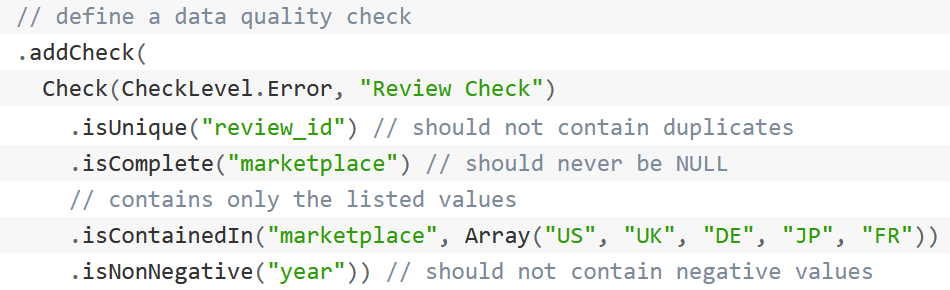
Figure 1. Example code snippet to describe expected data-values, using declarative constraints in Amazon Deequ.

Automate Data Validation using Inferred Constraints. While declarative data validation clearly improves over ad-hoc scripts, and is beneficial as reported by both Google and Amazon (breck2019data, ; schelter2018automating, ), the need for data engineers to manually write data constraints one-column-at-a-time (e.g., in Figure 1) still makes it time-consuming and hard to scale. This is especially true for complex production data, where a single data feed can have hundreds of columns requiring substantial manual work. As a result, experts today can only afford to write validation rules for part of their data (e.g., important columns). Automating the generation of data validation constraints has become an important problem.

The main technical challenge here is that validation rules have to be inferred using data values currently observed from a pipeline, but the inferred rules have to apply to future data that cannot yet be observed (analogous to training-data/testing-data in ML settings where test-data cannot be observed). Ensuring that validation rules generalize to unseen future data is thus critical.

We should note that existing solutions already make efforts in this direction – both Google TFDV and Amazon Deequ can scan an existing data feed, and automatically suggest validation constraints for human engineers to inspect and approve. Our analysis suggests that the capabilities of these existing solutions are still rudimentary, especially on string-valued data columns. For instance, for the example $C_{1}$ in Figure 2(a) with date strings in Mar 2019, TFDV would infer a validation rule requiring all future values in this column to come from a fixed dictionary with existing values in $C_{1}$: {“ Mar 01 2019”, …“ Mar 30 2019” }. This is too restrictive for data validation, as it can trigger false-alarms on future data (e.g. values like “Apr 01 2019”). Accordingly, TFDV documentation does not recommend suggested rules to be used directly, and “strongly advised developers to review the inferred rule and refine it as needed”.

When evaluated on production data (without human intervention), we find TFDV produces false-alarms on over 90% string-valued columns. Amazon’s Deequ considers distributions of values but still falls short, triggering false-alarms on over 20% columns. Given that millions of data columns are processed daily in production systems, these false-positive rates can translate to millions of false-alarms, which is not adequate for automated applications.

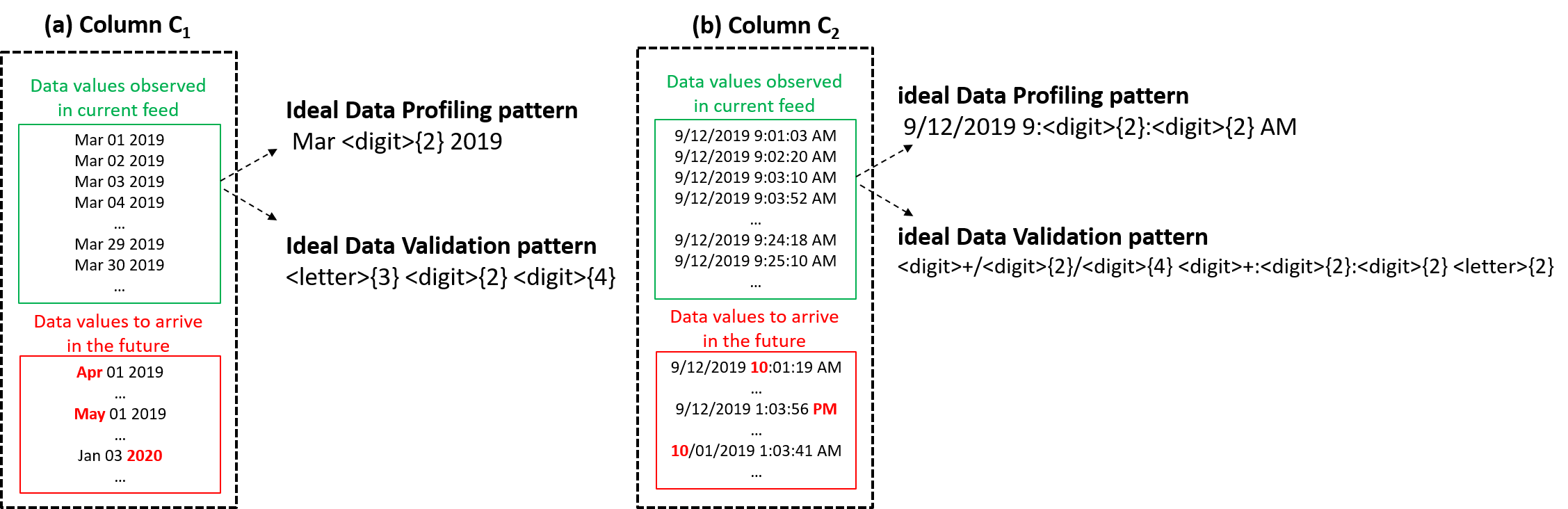
Figure 2. Two example data columns $C_{1}$ and $C_{2}$. The top portion of each column shows data in the current feed that can be observed, while the bottom portion shows values that will arrive in the future.

Auto-Validate string-valued data using patterns. We in this work aim to infer accurate data-validation rules for string-valued data, using regex-like patterns. We perform an in-depth analysis of production data in real pipelines, from a large Map-Reduce-like system used at Microsoft (patel2019big, ; zhou2012scope, ), which hosts over 100K production jobs each day, and powers popular products like Bing Search and Office. We crawl a sample of 7M columns from the data lake hosting these pipelines and find string-valued columns to be prevalent, accounting for 75% of columns sampled.

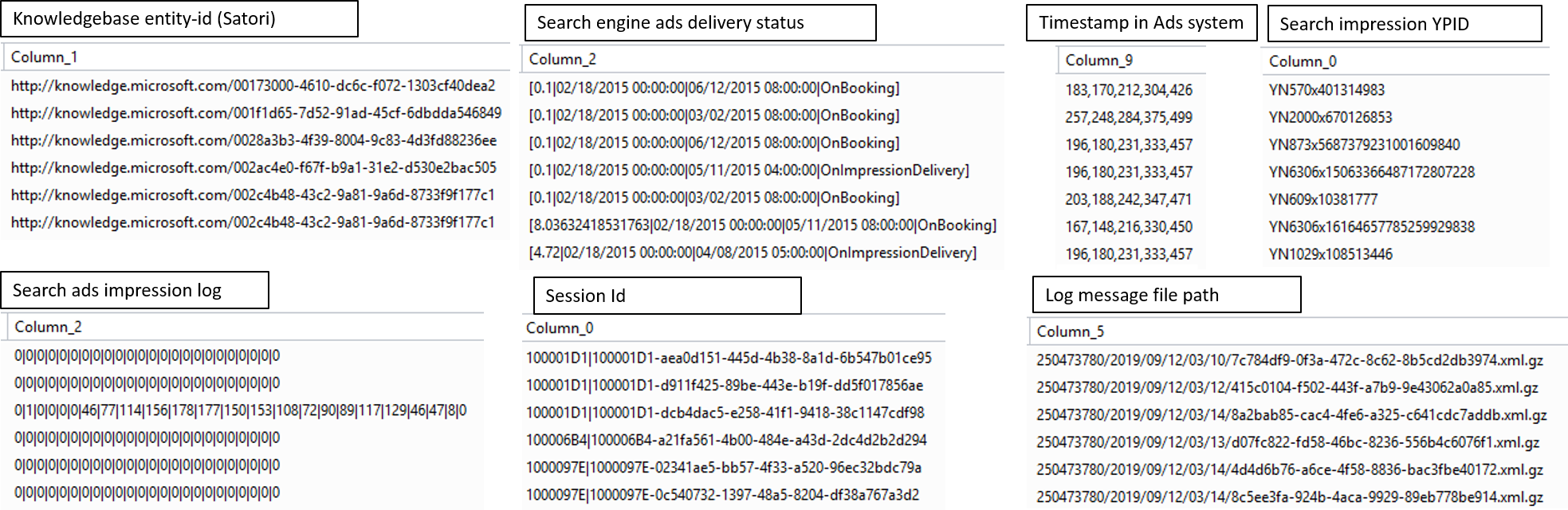
Figure 3. Example columns crawled from a production enterprise data lake. Each column has a distinctive data pattern in proprietary formats, encoding specific meanings (the first column is anonymized for review). These are all common patterns found in at least 5000 columns.

Figure 3 shows 7 example string-valued columns from the crawl. A key characteristic common to many such columns, is that these columns have homogeneous and machine-generated data values, which exhibit distinct “patterns” that encode specific semantic meanings. In our examples, these include knowledge-base entity-id (BingEntity, ) (used by Bing Search), online-ads delivery status (used by search ads), time-stamps in proprietary formats (used by search ads), etc. We note that these are not one-off patterns occurring just once or twice – each pattern in Figure 3 shows up in at least 5000 data columns in our crawl, suggesting that these are widely-used concepts. Similar data are likely common in other industries and domains (e.g., for pharmaceutical or financial companies (stonebraker2018data, )).

In this work, we focus on these string-valued columns that have homogeneous machine-generated data values. Specifically, if we could infer suitable patterns to describe the underlying “domain” of the data (defined as the space of all valid values), we can use such patterns as validation rules against data in the future. For instance, the pattern “<letter>{3} <digit>{2} <digit>{4}” can be used to validate $C_{1}$ in Figure 2(a), and “<digit>+/<digit>{2}/<digit>{4} <digit>+:<digit>{2}:<digit>{2} <letter>{2}” for $C_{2}$ in Figure 2(b).

Our analysis on a random sample of 1000 columns from our production data lake suggests that around 67% string-valued columns have homogeneous machine-generated values (like shown in Figure 3), whose underlying data-domains are amenable to pattern-based representations (the focus of this work). The remaining 33% columns have natural-language (NL) content (e.g., company names, department names, etc.), for which pattern-based approaches would be less well-suited. We should emphasize that for large data-lakes and production data pipelines, machine-generated data will likely dominate (because machines are after all more productive at churning out large volumes of data than humans producing NL data), making our proposed technique widely applicable.

While on the surface this looks similar to prior work on pattern-profiling (e.g., Potter’s Wheel (raman2001potter, ) and PADS (fisher2005pads, )), which also learn patterns from values, we highlight the key differences in their objectives that make the two entirely different problems.

Data Profiling vs. Data Validation. In pattern-based data profiling, the main objective is to “summarize” a large number of values in a column $C$, so that users can quickly understand content is in the column without needing to scroll/inspect every value. As such, the key criterion is to select patterns that can succinctly describe given data values in $C$ only, without needing to consider values not present in $C$.

For example, existing pattern profiling methods like Potter’s Wheel (raman2001potter, ) would correctly generate a desirable pattern “Mar <digit>{2} 2019” for $C_{1}$ in Figure 2(a), which is valuable from a pattern-profiling’s perspective as it succinctly describes values in $C_{1}$. However, this pattern is not suitable for data-validation, as it is overly-restrictive and would trigger false-alarms for values like “Apr 01 2019” arriving in the future. A more appropriate data-validation pattern should instead be “<letter>{3} <digit>{2} <digit>{4}”. Similarly, for $C_{2}$, Figure 2(b) shows that a pattern ideal for profiling is again very different from one suitable for data-validation.

Figure 4. Example string generalization hierarchy.

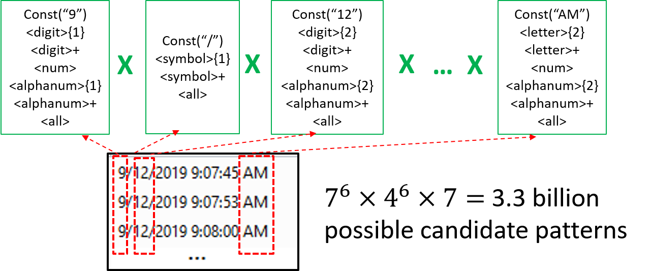
Figure 5. Possible ways to generalize a column of date-time strings, using the hierarchy in Figure 4.

Conceptually, there are many ways to “generalize” a column of data into patterns. For a simple column of date-time strings like in Figure 5, and using a standard generalization hierarchy (Figure 4), one could generate over 3 billion patterns. For example, the first part (digit “9” for month) alone can be generalized in 7 different ways below, also shown in the top-right box of Figure 5.

• (1) a constant “9” (Const(‘‘9’’)),

• (2) one single digit (<digit>{1}),

• (3) at least one digits (<digit>+),

• (4) any number including floating-points (<num>),

• (5) one alpha-numeric character (<alphanum>),

• (6) at least one alpha-numeric characters (<alphanum>+),

• (7) root of the hierarchy (<all>)

The cross-product of these options at each position creates a large space of patterns (about 3.3 billion) for this simple column.

The challenge for data-validation, is to select suitable patterns from this large space given only observed values in $C$, in anticipation of valid values from the same “domain” that may arrive in the future. The key is to not use overly restrictive patterns (as in data-profiling), which would yield many false-positive alerts. Conversely overly general patterns (like the trivial “.*”) should also not be used, as they would fail to detect any data quality issues. In effect, we want to find patterns that balance two conflicting goals: (1) reduce false-alarms (or improve detection precision); and (2) catch as many issues as possible (or improve detection recall).

A corpus-driven approach to pattern-inference. Intuitively, the pattern-inference problem is hard if we only look at one input column $C$ – for the date-time examples in Figure 2, we as humans know what patterns are suitable; but for the examples in Figure 3 drawn from proprietary domains, even humans may find it hard to determine suitable validation patterns, and would need to seek “additional evidence”, such as other “similar-looking columns”.

Following this intuition, we in this work formulate pattern-inference as optimization problems, by leveraging a large corpus of related tables $\mathbf{T}$ (e.g. data produced by production pipelines and dumped in the same enterprise data lake). Our inference algorithms leverage columns “similar” to $C$ in $\mathbf{T}$, to reason about patterns that may be ideal for data-validation.

Large-scale evaluations on production data suggest that Auto-Validate produces constraints that are substantially more accurate than existing methods. Part of this technology ships as an Auto-Tag feature in Microsoft Azure Purview (purview, ).

2. Auto-Validate (Basic Version)

We start by describing a basic-version of Auto-Validate for ease of illustration, before going into more involved algorithm variants that use vertical-cuts (Section 3) and horizontal-cuts (Section 4).

2.1. Preliminary: Pattern Language

Since we propose to validate data by patterns, we first briefly describe the pattern language used. We note that this is fairly standard (e.g., similar to ones used in (raman2001potter, )) and not the focus of this work.

Figure 4 shows a generalization hierarchy used, where leaf-nodes represent the English alphabet, and intermediate nodes (e.g., <digit>, <letter>) represent tokens that values can generalize into. A pattern is simply a sequence of (leaf or intermediate) tokens, and for a given value $v$, this hierarchy induces a space of all patterns consistent with $v$, denoted by $\mathbf{P}(v)$. For instance, for a value $v=$ “9:07”, we can generate $\mathbf{P}(v)=$ {“<digit>:<digit>{2}”, “<digit>+:<digit>{2}”, “<digit>:<digit>+”, “<num>:<digit>+”, “9:<digit>{2}”, …}, among many other options.

Given a column $C$ for which patterns need to be generated, we define the space of hypothesis-patterns, denoted by $\mathbf{H}(C)$, as the set of patterns consistent with all values $v\in C$, or $\mathbf{H}(C)=\cap_{v\in C}{\mathbf{P}(v)}\setminus\text{``.*''}$ (note that we exclude the trivial “.*” pattern as it is trivially consistent with all $C$). Here we make an implicit assumption that values in $C$ are homogeneous and drawn from the same domain, which is generally true for machine-generated data from production pipelines (like shown in Figure 3). Note that the assumption is used to only simplify our discussion of the basic-version of Auto-Validate (this section), and will later be relaxed in more advanced variants (Section 4).

We call $\mathbf{H}(C)$ hypothesis-patterns because as we will see, each $h(C)\in\mathbf{H}(C)$ will be tested like a “hypothesis” to determine if $h$ is a good validation pattern. We use $h$ and $h(C)$ interchangeably when the context is clear.

Example 1.

Given the column $C$ shown in Figure 5, and the hierarchy in Figure 4, the space of hypothesis patterns $\mathbf{H}(C)$ is shown at the top of Figure 5.

We use an in-house implementation to produce patterns based on the hierarchy, which can be considered as a variant of well-known pattern-profiling techniques like (raman2001potter, ). Briefly, our pattern-generation works in two steps. In the first step, it scans each cell value and emits coarse-grained tokens (e.g., <num> and <letter>+), without specializing into fine-grained tokens (e.g., <digit>{1} or <letter>{2}). For each value in Figure 5, for instance, this produces the same <num>/<num>/<num> <num>:<num>:<num> <letter>+. Each coarse-grained pattern is then checked for coverage so that only patterns meeting a coverage threshold are retained. In the second step, each coarse-grained pattern is specialized into fine-grained patterns (examples are shown in Figure 5), as long as the given threshold is met. Pseudo-code of the procedure can be found in Algorithm 1 below.

GeneratePatterns $(\textnormal{{$\mathcal{S}$}},H)$

       input : string values $\textnormal{{$\mathcal{S}$}}=\{s_{1},\dots,s_{n}\}$, generalization hierarchy $H$

       output : patterns $\textnormal{{$\mathcal{P}$}}_{fine}$ of $\mathcal{S}$ induced by $H$

       $\textnormal{{$\mathcal{P}$}}_{coarse}\leftarrow\{\}$;

       foreach $s\in\textnormal{{$\mathcal{S}$}}$  do

             p $\leftarrow$ GenerateCoarsePatterns(s);

             add p to $\textnormal{{$\mathcal{P}$}}_{coarse}$

       end foreach

      retain patterns in $\textnormal{{$\mathcal{P}$}}_{coarse}$ with sufficient coverage;

       $\textnormal{{$\mathcal{P}$}}_{fine}\leftarrow\{\}$;

       foreach $p$ $\in$ $\textnormal{{$\mathcal{P}$}}_{coarse}$ do

             p’ $\leftarrow$ drill-down each $p$ using $H$;

             add p’ to $\textnormal{{$\mathcal{P}$}}_{fine}$ if coverage is sufficient ;

            

       end foreach

      return $\textnormal{{$\mathcal{P}$}}_{fine}$;

      

Algorithm 1 Generate patterns from a column of values

We emphasize that the proposed Auto-Validate framework is not tied to specific choices of hierarchy/pattern-languages – in fact, it is entirely orthogonal to such choices, as other variants of languages are equally applicable in this framework.

2.2. Intuition: Goodness of Patterns

The core challenge in Auto-Validate, is to determine whether a pattern $h(C)\in\mathbf{H}(C)$ is suitable for data-validation. Our idea here is to leverage a corpus of related tables $\mathbf{T}$ (e.g., drawn from the same enterprise data lake, which stores input/output data of all production pipelines). Intuitively, a pattern $h(C)\in\mathbf{H}(C)$ is a “good” validation pattern for $C$, if it accurately describes the underlying “domain” of $C$, defined as the space of all valid data values. Conversely, $h(C)$ is a “bad” validation pattern, if:

• (1) $h(C)$ does not capture all valid values in the underlying “domain” of $C$;

• (2) $h(C)$ does not produce sufficient matches in $\mathbf{T}$.

Both are intuitive requirements – (1) is desirable, because as we discussed, the danger in data-validation is to produce patterns that do not cover all valid values from the same domain, which leads to false alarms. Requirement (2) is also sensible because we want to see sufficient evidence in $\mathbf{T}$ before we can reliably declare a pattern $h(C)$ to be a common “domain” of interest (seeing a pattern once or twice is not sufficient).

We note that both of these two requirements can be reliably tested using $\mathbf{T}$ alone and without involving humans. Testing (2) is straightforward using standard pattern-matches. Testing (1) is also feasible, under the assumption that most data columns in $D\in\mathbf{T}$ contain homogeneous values drawn from the same underlying domain, which is generally true for “machine-generated” data from production pipelines. (Homogeneity is less likely to hold on other types of data, e.g., data manually typed in by human operators).

We highlight the fact that we are now dealing with two types of columns that can be a bit confusing – the first is the input column $C$ for which we need to generate validation patterns $h$, and the second is columns $D\in\mathbf{T}$ from which we draw evidence to determine the goodness of $h$. To avoid confusion, we will follow the standard of referring to the first as the query column, denoted by $C$, and the second as data columns, denoted by $D$.

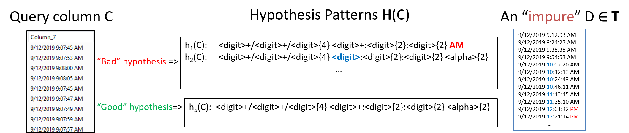
Figure 6. Leverage corpus $\mathbf{T}$ to determine “good” vs. “bad” hypothesis patterns, for a given query column $C$.

We now show how to test requirement (1) using $\mathbf{T}$ below.

Example 2.

The left of Figure 6 shows a query column $C$ for which validation patterns need to be generated. A few hypothesis-patterns in $\mathbf{H}(C)$ are listed in the middle. In this example, we intuitively know that $h_{1}(C)$ and $h_{2}(C)$ are “bad” patterns since they are too “narrow” and would lead to false-alarms, while $h_{5}(C)$ is a “good” validation pattern that suitably generalizes the underlying domain.

We show that such determinations can be inferred using $\mathbf{T}$. Specifically, $h_{1}(C)$ is a “bad” pattern based on $\mathbf{T}$, because we can find many columns like $D\in\mathbf{T}$ shown on the right of Figure 6 that are “impure” – these columns contain values that match $h_{1}(C)$, as well as values that do not (e.g., “9/12/2019 12:01:32 PM”, where the “PM” part does not match $h_{1}(C)$). A large number of “impure” columns like this would indicate that $h_{1}(C)$ is not a good pattern to describe the underlying domain because if it were, we should not see many impure columns like $D\in\mathbf{T}$ given homogeneity.

Similarly, we can show that $h_{2}(C)$ is not a good validation pattern, for using $h_{2}(C)$ to describe the domain would again make many columns like $D$ “impure” (values like “10:02:20 AM” are inconsistent with $h_{2}(C)$ since they have two-digit hours, whereas $h_{2}(C)$ uses a single <digit> for hours), suggesting $h_{2}(C)$ is also too narrow.

Using the ideal pattern $h_{5}(C)$ to describe the domain, on the other hand, would yield few “impure” columns in $\mathbf{T}$.

Intuitively, we can use the impurity of pattern $h$ on data columns $D\in\mathbf{T}$, to infer whether $h$ is a good validation pattern for the domain, defined as follows.

Definition 3.

The impurity of a data column $D\in\mathbf{T}$, relative to a given hypothesis pattern $h$, is defined as:

(1) $$\text{Imp}_{D}(h)=\frac{|\{v|v\in D,h\notin\mathbf{P}(v)\}|}{|\{v|v\in D\}|}$$

This definition is intuitive – we measure impurity as the fraction of values in $D$ not matching $h$.

Example 4.

In Figure 6, $\text{Imp}_{D}(h_{1})$ can be calculated as $\frac{2}{12}$, since the last 2 values (with “PM”) out of 12 do not match $h_{1}$.

Similarly, $\text{Imp}_{D}(h_{2})$ can be calculated as $\frac{8}{12}$, since the last 8 values in $D$ (with two-digit hours) do not match $h_{2}$.

Finally, $\text{Imp}_{D}(h_{5})$ is $\frac{0}{12}$, since all values in $D$ match $h_{5}$.

We note that if $h(C)$ is used to validate a data column $D$ (in the same domain as $C$) arriving in the future, then Imp${}_{D}(h)$ directly corresponds to expected false-positive-rate (FPR):

Definition 5.

The expected false-positive-rate (FPR) of using pattern $h(C)$ to validate a data column $D$ drawn from the same domain as $C$, denoted by $\text{FPR}_{D}(h)$, is defined as:

(2) $$\text{FPR}_{D}(h)=\frac{\text{FP}_{D}(h)}{\text{TN}_{D}(h)+\text{FP}_{D}(h)}$$

Where FP${}_{D}(h)$ and TN${}_{D}(h)$ are the numbers of false-positive detection and true-negative detection of $h$ on $D$, respectively.

Note that since $D$ is from the same domain as $C$, ensuring that TN${}_{D}(h)$ + FP${}_{D}(h)$ = $|D|$, $\text{FPR}_{D}(h)$ can be rewritten as:

(3) $$\text{FPR}_{D}(h)=\frac{|\{v|v\in D,h\notin\mathbf{P}(v)\}|}{|\{v|v\in D\}|}=\text{Imp}_{D}(h)$$

Thus allowing us to estimate $\text{FPR}_{D}(h)$ using $\text{Imp}_{D}(h)$.

Example 6.

Continue with Example 4, it can be verified that the expected FPR of using $h$ as the validation pattern for $D$, directly corresponds to the impurity $\text{Imp}_{D}(h)$ – e.g., using $h_{1}$ to validate $D$ has $\text{FPR}_{D}(h_{1})$ = $\text{Imp}_{D}(h_{1})$ = $\frac{2}{12}$; while using $h_{5}$ to validate $D$ has $\text{FPR}_{D}(h_{5})=\text{Imp}_{D}(h_{5})=0$, etc.

Based on FPR${}_{D}(h)$ defined for one column $D\in\mathbf{T}$, we can in turn define the estimated FPR on the entire corpus $\mathbf{T}$, using all column $D\in\mathbf{T}$ where some value $v\in D$ matches $h$:

Definition 7.

Given a corpus $\mathbf{T}$, we estimate the FPR of pattern $h$ on $\mathbf{T}$, denoted by FPR${}_{\mathbf{T}}(h)$, as:

(4) $$\text{FPR}_{\mathbf{T}}(h)=\operatorname*{avg}_{D\in\mathbf{T},v\in D,h\in\mathbf{P}(v)}{\text{FPR}_{D}(h)}$$

Example 8.

Continue with the $h_{5}$ in Example 6. Suppose there are 5000 data columns $D\in\mathbf{T}$ where some value $v\in D$ matches $h_{5}$. Suppose 4800 columns out of the 5000 have $\text{FPR}_{D}(h_{5})=0$, and the remaining 200 columns have $\text{FPR}_{D}(h_{5})=1\%$. The overall $\text{FPR}_{\mathbf{T}}(h_{5})$ can be calculated as $\frac{200*1\%}{5000}=0.04\%$, using Equation (4).

We emphasize that a low FPR is critical for data-validation, because given a large number of columns in production systems, even a 1% FPR translates into many false-alarms that require human attention to resolve. FPR is thus a key objective we minimize.

2.3. Problem Statement

We now describe the basic version of Auto-Validate as follows. Given an input query column $C$ and a background corpus $\mathbf{T}$, we need to produce a validation pattern $h(C)$, such that $h(C)$ is expected to have a low FPR but can still catch many quality issues. We formulate this as an optimization problem. Specifically, we introduce an FPR-Minimizing version of Data-Validation (FMDV), defined as:

(5) $$\text{(FMDV)}\qquad{}\min_{h\in\mathbf{H}(C)} \text{FPR}_{\mathbf{T}}(h)$$

(6) s.t. $$\text{FPR}_{\mathbf{T}}(h)\leq r$$

(7) $$\text{Cov}_{\mathbf{T}}(h)\geq m$$

Where $\text{FPR}_{\mathbf{T}}(h)$ is the expected FPR of $h$ estimated using $\mathbf{T}$, which has to be lower than a given target threshold $r$ (Equation (6)); and $\text{Cov}_{\mathbf{T}}(h)$ is the coverage of $h$, or the number of columns in $\mathbf{T}$ that match $h$, which has to be greater than a given threshold $m$ (Equation (7)). Note that these two constraints directly map to the two “goodness” criteria in Section 2.2.

The validation pattern $h$ we produce for $C$ is then the minimizer of FMDV from the hypothesis space $\mathbf{H}(C)$ (Equation (5)). We note that this can be interpreted as a conservative approach that aims to find a “safe” pattern $h(C)$ with minimum FPR.

Example 9.

Suppose we have FMDV with a target FPR rate $r$ no greater than $0.1\%$, and a required coverage of at least $m=100$. Given the 3 example hypothesis patterns in Figure 6, we can see that patterns $h_{1}$ and $h_{2}$ are not feasible solutions because of their high estimated FPR. Pattern $h_{5}$ has an estimated FPR of 0.04% and a coverage of 5000, which is a feasible solution to FMDV.

Lemma 10.

In a simplified scenario where each column in $\mathbf{T}$ has values drawn randomly from exactly one underlying domain, and each domain in turn corresponds to one ground-truth pattern. Then given a query column $C$ for which a validation pattern needs to be generated, and a corpus $\mathbf{T}$ with a large number ($n$) of columns generated from the same domain as $C$, with high probability (at least $1-(\frac{1}{2})^{n}$), the optimal solution of FMDV for $C$ (with $r=0$) converges to the ground-truth pattern of $C$.

Proof Sketch: We show that any candidate patterns that “under-generalizes” the domain will with high probability be pruned away due to FPR violations (given $r=0$). To see why this is the case, consider a pattern $p$ produced for $C$ that under-generalizes the ground-truth pattern $g$. Note $p$ is picked over $g$ only when not a single value in all $n$ columns in the same domain as $C$ drawn from the space of values defined by $g$ are not in $p$ (since $r$ is set to 0). Because these $n$ columns are drawn randomly from $g$ and each column has at least one value, the probability of this happening is thus at most $(\frac{1}{2})^{n}$ ($\frac{1}{2}$ is used because there is at least one branch $p^{\prime}$ in $g$ that is not in $p$), making the overall probability of success to be $1-(\frac{1}{2})^{n}$. ∎

We also explored alternative formulations, such as coverage-minimizing data-validation (CMDV), where we minimize coverage $\text{Cov}_{\mathbf{T}}(h)$ in the objective function in place of FPR${}_{\mathbf{T}}(h)$ as in FMDV. We omit details in the interest of space, but will report that the conservative FMDV is more effective in practice.

A dual version of FMDV can be used for automated data-tagging, where we want to find the most restrictive (smallest coverage) pattern to describe the underlying domain (which can be used to “tag” related columns of the same type), under the constraint of some target false-negative rate. We describe this dual version in (auto-tag-tr, ).

2.4. System Architecture

While FMDV is simple overall, a naive implementation would require a full scan of $\mathbf{T}$ to compute $\text{FPR}_{\mathbf{T}}(h)$ and $\text{Cov}_{\mathbf{T}}(h)$ for each hypothesis $h$. This is both costly and slow considering the fact that $\mathbf{T}$ is typically large in enterprise data lakes (e.g., in terabytes), where a full-scan can take hours. This is especially problematic for user-in-the-loop validation like in Google’s TFDV, where users are expected to review/modify suggested validation rules and interactive response time is critical.

We thus introduce an offline index with summary statistics of $\mathbf{T}$, so that at online time and given a new query column $C$, we can evaluate hypothesis patterns $h$ efficiently using only the index, without needing to scan $\mathbf{T}$ again.

The architecture of our system can be seen in Figure 7.

Offline stage. In the offline stage, we perform one full scan of $\mathbf{T}$, enumerating all possible patterns for each $D\in\mathbf{T}$ as $\mathbf{P}(D)=\cup_{v\in D}\mathbf{P}(v)$, or the union of patterns for all $v\in D$ (where $\mathbf{P}$ is the generalization hierarchy in Section 2.1).

Note that the space of $\mathbf{P}(D)$ can be quite large, especially for “wide” columns with many tokens as discussed in Figure 5. To limit $\mathbf{P}(D)$, in the basic version we produce $\mathbf{P}(D)$ as $\cup_{v\in D,t(v)<\tau}\mathbf{P}(v)$, where $t(v)$ is the number of tokens in $v$ (defined as the number of consecutive sequences of letters, digits, or symbols in $v$), and $\tau$ is some fixed constant (e.g., 8 or 13) to make $\mathbf{P}(D)$ tractable. We will describe how columns wider than $\tau$ can be safely skipped in offline indexing without affecting result quality, using a vertical-cut technique (in Section 3).

For each pattern $p\in\mathbf{P}(D)$, we pre-compute the local impurity score of $p$ on $D$ as $\text{Imp}_{D}(p)$, since $p$ may be hypothesized as a domain pattern for some query column $C$ in the future, for which this $D$ can provide a piece of local evidence.

Let $\mathbf{P}(\mathbf{T})=\{p|p\in\mathbf{P}(D),D\in\mathbf{T}\}$ be the space of possible patterns in $\mathbf{T}$. We pre-compute $\text{FPR}_{\mathbf{T}}(p)$ for all possible $p\in\mathbf{P}(\mathbf{T})$ on the entire $\mathbf{T}$, by aggregating local $\text{Imp}_{D}(p)$ scores using Equation (3) and (4). The coverage scores $\text{Cov}_{\mathbf{T}}(p)$ of all $p$ can be pre-computed similarly as $\text{Cov}_{\mathbf{T}}(p)=|\{D|D\in\mathbf{T},v\in D,p\in\mathbf{P}(v)\}|$.

The result from the offline step is an index for lookup that maps each possible $p\in\mathbf{P}(\mathbf{T})$, to its pre-computed $\text{FPR}_{\mathbf{T}}(p)$ and $\text{Cov}_{\mathbf{T}}(p)$ values. We note that this index is many orders of magnitude smaller than the original $\mathbf{T}$ – e.g., a 1TB corpus $\mathbf{T}$ yields an index less than 1GB in our experiments.

Online stage. At online query time, for a given query column $C$, we enumerate $h\in\mathbf{H}(C)$, and use the offline index to perform a lookup to retrieve $\text{FPR}_{\mathbf{T}}(p)$ and $\text{Cov}_{\mathbf{T}}(p)$ scores for FMDV, without needing to scan the full $\mathbf{T}$ again. This indexing approach reduces our latency per query-column $C$ from hours to tens of milliseconds, which makes it possible to do interactive, human-in-the-loop verification of suggested rules, as we will report in experiments.

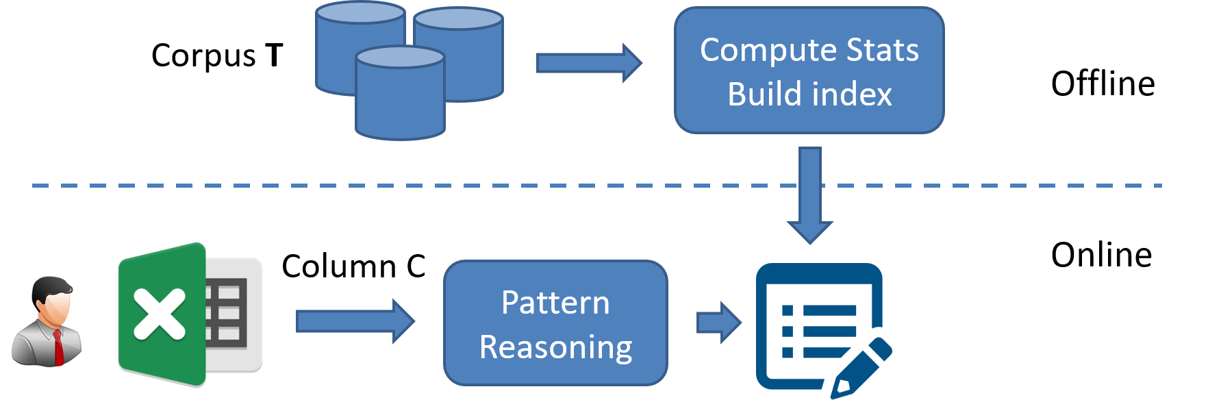
Figure 7. Architecture of the Auto-Validate System.

3. Auto-Validate (Vertical Cuts)

So far we only discussed the basic-version of Auto-Validate. We now describe formulations that handle more complex and real situations: (1) composite structures in query columns (this section); and (2) “dirty” values in query columns that violate the homogeneity assumption (Section 4).

Figure 8 shows a real column with composite structures that are concatenated from atomic domains. Intuitively, we can see that it consists of at least 4 “sub-domains”, a floating-number (“0.1”), followed by two time-stamps, followed by a status message (“OnBooking”). We observe that such columns are common in machine-generated data, where many are complex with over 10 sub-domains.

Such complex columns pose both quality and scalability challenges. In terms of quality, if we were to directly test complex patterns against $\mathbf{T}$ like in FMDV, we may not be able to see many exact matches in $\mathbf{T}$, because the complex patterns in $C$ may be concatenated in ad-hoc ways and are sparsely represented in $\mathbf{T}$. As a result, we may fail to find a feasible solution to FMDV, because of the coverage requirement in Equation (7).

The second challenge is scalability. As column $C$ become “wider” with more tokens/segments, the space of possible patterns $\mathbf{P}(C)$ that we will have to enumerate grows exponentially in the number of tokens. This is an issue both at online query time for query column $C$, as well as at offline indexing time to enumerate $\mathbf{P}(D)$ for data column $D\in\mathbf{T}$ – recall that the date-time example in Figure 5 already produces over 3 billion patterns; for the column in Figure 8 the space of patterns is simply impractically large to enumerate. In the offline indexing step in Section 2.4, we discussed that we intentionally omit wide columns with more than $\tau$ tokens to make pattern enumeration tractable. We will show here that our horizontal-cut algorithm can “compensate” such omission without affecting result quality.

A natural approach to complex query column $C$ is to vertically “cut” it into sub-columns (like shown in Figure 8). Patterns for each sub-column can then be generated in turn using FMDV. The benefit of this divide-and-conquer approach is that each sub-domain is likely well-represented in $\mathbf{T}$, allowing them to be reliably inferred from $\mathbf{T}$. Furthermore, the cost of pattern-enumeration in offline-indexing becomes significantly smaller, as each sub-domain can be enumerated separately.

Specifically, we first use a lexer to tokenize each $v\in C$ into coarse-grained token-class (<symbol>, <num>, <letter>), by scanning each $v$ from left to right and “growing” each token until a character of a different class is encountered. In the example of Figure 8, for each row, we would generate an identical token-sequence “[<num>|<num>/<num>/<num> <num>:<num>:<num>| …|<letter>]”.

We then perform multi-sequence alignment (MSA) (carrillo1988multiple, ) for all token sequences, before actually performing vertical-cuts. Recall that the goal of MSA is to find optimal alignment across all input sequences (using objective functions such as sum-of-pair scores (just2001computational, )). Since MSA is NP-hard in general (just2001computational, ), we follow a standard approach to greedily align one additional sequence at a time. We note that for homogeneous machine-generated data, this often solves MSA optimally.

Example 1.

For the column in Figure 8, each value $v\in C$ has an identical token-sequence with 29 tokens: “[<num>|<num>/<num>/<num> <num>:<num>:<num>| …|<letter>]”, and the aligned sequence using MSA can be produced trivially as just a sequence with these 29 tokens (no gaps).

After alignment, characters in each $v\in C$ would map to the aligned sequence of length $n$ (e.g., “0.1” maps to the first <num> in the aligned token sequence, “02” maps to the second <num>, etc.). Recall that our goal is to vertically split the $n$ tokens into $m$ segments so that values mapped to each segment would correspond to a sub-domain as determined by FMDV. We define an $m$-segmentation of $C$ as follows.

Definition 2.

Given a column $C$ with $n$ aligned tokens, define $C[s,e]$ as a segment of $C$ that starts from token position $s$ and ends at position $e$, with $s,e\in[n]$. An $m$-segmentation of $C$, is a list of $m$ such segments that collectively cover $C$, defined as: $(C[s_{1},e_{1}],C[s_{2},e_{2}],$ $\ldots$ $C[s_{m},e_{m}])$, where $s_{1}=1,e_{m}=n$, and $s_{i+1}=e_{i}+1~{}\forall i\in[m]$. We write $C[s_{i},e_{i}]$ as $C_{i}$ for short, and an $m$-segmentation as $(C_{i}:i\in[m])$ for short.

Note that each $C_{i}$ can be seen just like a regular column “cut” from the original $C$, with which we can invoke the FMDV. Our overall objective is to jointly find: (1) an $m$-segmentation $(C_{i}:i\in[m])$ from all possible segmentation, denoted by $\mathbf{S}(C)$; and (2) furthermore find appropriate patterns $h_{i}\in\mathbf{H}(C_{i})$ for each segment $C_{i}$, such that the entire $C$ can be validated with a low expected FPR. Also note that because we limit pattern enumeration in offline-indexing to columns of at most $\tau$ tokens, we would not find candidate patterns longer than $\tau$ in offline-index, and can thus naturally limit the span of each segment to at most $\tau$ ($e_{i}-s_{i}<\tau$, $\forall i$). We can write this as an optimization problem FMDV-V defined as follows:

(8) $$\text{(FMDV-V)}~{}\min_{\begin{subarray}{c}h_{1}\dots h_{m}\\ h_{i}\in\mathbf{H}(C_{i})\\ (C_{i}:i\in[m])\in\mathbf{S}(C)\end{subarray}}~{}~{}~{} \sum_{h_{i}}\text{FPR}_{\mathbf{T}}(h_{i})$$

(9) s.t. $$\sum_{h_{i}}\text{FPR}_{\mathbf{T}}(h_{i})\leq r$$

(10) $$\text{Cov}_{\mathbf{T}}(h_{i})\geq m,~{}\forall h_{i}$$

In FMDV-V, we are optimizing over all possible segmentation $(C_{i}:i\in[m])\in\mathbf{S}(C)$, and for each $C_{i}$ all possible hypothesis patterns $h_{i}\in\mathbf{H}(C_{i})$. Our objective in Equation (8) is to minimize the sum of $\text{FPR}_{\mathbf{T}}(h_{i})$ for all $h_{i}$. We should note that this corresponds to a “pessimistic” approach that assumes non-conforming rows of each $h_{i}$ are disjoint at a row-level, thus needing to sum them up in the objective function. (An alternative could “optimistically” assume non-conforming values in different segments to overlap at a row-level, in which case we can use max in place of the sum. We find this to be less effective and omit details in the interest of space).

We can show that the minimum FRP scores of $m$-segmentation optimized in Equation (8) have optimal substructure (cormen2009introduction, ), which makes it amenable to dynamic programming (without exhaustive enumeration). Specifically, we can show that the following holds:

(11) $$\begin{split}\text{minFRP}&(C[s,e])=\\ \min\bigg{(}&\min_{h\in\mathbf{P}(C[s,e])}\text{FPR}_{\mathbf{T}}(h),\\ &\min_{t\in[s,e-1]}{\Big{(}\text{minFPR}(C[s,t])+\text{minFPR}(C[t+1,e])\Big{)}}\bigg{)}\end{split}$$

Here, minFRP$(C[s,e])$ is the minimum FRP score with vertical splits as optimized in Equation (8), for a sub-column corresponding to the segment $C[s,e]$ from token-position $s$ to $e$. Note that $C[1,n]$ corresponds to the original query column $C$, and minFRP$(C[1,n])$ is the score we want to optimize. Equation (11) shows how this can be computed incrementally. Specifically, minFRP$(C[s,e])$ is the minimum of (1) $\min_{h\in\mathbf{P}(C[s,e])}\text{FPR}_{\mathbf{T}}(h)$, which is the FRP score of treating $C[s,e]$ as one column (with no splits), solvable using FMDV; and (2) $\min_{t\in[s,e-1]}{\big{(}\text{minFPR}(C[s,t])+\text{minFPR}(C[t+1,e])\big{)}}$, which is the best minFRP scores from all possible two-way splits that can be solved optimally in polynomial time using bottom-up dynamic-programming.

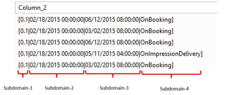
Figure 8. Example columns with composite domains.

Example 3.

Continue with Example 1. The aligned sequence of column $C$ in Figure 8 has 29 tokens, corresponding to $C[1,29]$. The sub-sequence $C[4,14]$ maps to identical values “02/18/2015 00:00:00” for all rows, which can be seen as a “sub-column” split from $C$.

Using Equation (11), minFRP$(C[4,14])$ of this sub-column can be computed as the minimum of: (1) Not splitting of $C[4,14]$, or $\min_{h\in\mathbf{P}(C[4,14])}\text{FPR}_{\mathbf{T}}(h)$, computed using FMDV; and (2) Further splitting $C[4,14]$ into two parts, where the best score is computed as $\min_{t\in[4,13]}{\Big{(}\text{minFPR}(C[4,t])+\text{minFPR}(C[t+1,14])\Big{)}}$, which can in turn be recursively computed. Suppose we compute (1) to have FPR of 0.004%, and the best of (2) to have FPR of 0.01% (say, splitting into “02/18/2015” and “00:00:00”). Overall, not splitting $C[4,14]$ is the best option.

Each such $C[s,e]$ can be computed bottom-up, until reaching the top-level. The resulting split minimizes the overall FPR and is the solution to FMDV-V.

We would like to highlight that by using vertical-cuts, we can safely ignore wide columns with more than $\tau$ tokens during offline indexing (Section 2.4), without affecting result quality. As a concrete example, when we encounter a column like in Figure 8, brute-force enumeration would generate at least $4^{29}$ patterns, which is impractically large and thus omitted given a smaller token-length limit $\tau$ (e.g., 13) in offline indexing. However, when we encounter this column Figure 8 as a query column, we can still generate valid domain patterns with the help of vertical-cuts (like shown in Example 3), as long as each segment has at most $\tau$ tokens. Vertical-cuts thus greatly speed up offline-indexing as well as online-inference, without affecting result quality.

4. Auto-Validate (Horizontal Cuts)

So far we assumed the query column $C$ to be “clean” with homogeneous values drawn from the same domain (since they are generated by the same underlying program). While this is generally true, we observe that some columns can have ad-hoc special values (e.g., denoting null/empty-values) that do not follow the domain-pattern of $C$, as shown in Figure 9.

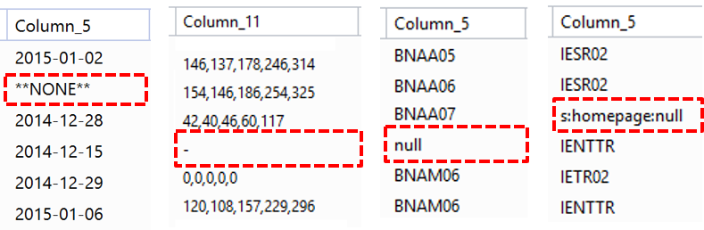
Figure 9. Example ad-hoc special values (in red boxes) not observing patterns of other values in the column.

We note that examples like these are not uncommon – even for machine-generated data, there can be a branch of logic (think of try-except) that handles special cases (e.g., nulls), and produces ad-hoc values not following the pattern of “normal” values. We henceforth refer to these as non-conforming values.

Recall that in FMDV, by assuming that the query column $C$ has homogeneous values, we select patterns from $\mathbf{H}(C)=\cap_{v\in C}{\mathbf{P}(v)}$, or the intersection of patterns for all values $v\in C$. Such an assumption does not hold for columns in Figure 9, yielding an empty $\mathbf{H}(C)$ and no feasible solution to FMDV.

We thus consider a variant of Auto-Validate with “horizontal cuts”, meaning that we can “cut off” a small fraction of non-conforming values in $C$ (which is identical to making patterns tolerate a small fraction of non-conforming values). We use a tolerance parameter $\theta$ to control the maximum allowed fraction of non-conforming values that can be cut (e.g., 1%, 5%, etc.), which allows for a conscious trade-off between precision and recall.

This optimization problem, termed FMDV-H, is defined as

(12) $$\text{(FMDV-H)}~{}~{}\min_{h}~{} \text{FPR}_{\mathbf{T}}(h)$$

(13) s.t. $$h\in\cup_{v\in C}{\mathbf{P}(v)\setminus\text{``.*''}}$$

(14) $$\text{FPR}_{\mathbf{T}}(h)\leq r$$

(15) $$\text{Cov}_{\mathbf{T}}(h)\geq m$$

(16) $$|\{v|v\in C,h\in\mathbf{P}(v)\}|\geq(1-\theta)|C|$$

Like before, our objective function is to minimize FPR in Equation (12). Equation (13) shows that the hypothesis pattern $h$ is drawn from the union of possible patterns for all $v\in C$. The FPR and Coverage requirements in Equation (14) and Equation (15) are the same as the basic FMDV. Finally, Equation (16) requires that the selected $h$ has to match at least $(1-\theta)$ fraction of values in $C$, where $\theta$ is the tolerance parameter above (the remaining $\theta$ fraction are non-conforming values).

Example 1.

Consider the leftmost column $C$ in Figure 9. Using FMDV-H, we determine the pattern $h=$ “<digit>+,<digit>+,<digit>+, <digit>+,<digit>+” to be a valid solution, as it meets the FPR and coverage requirements based on $\mathbf{T}$. Furthermore $h$ is consistent with 99% of values in $C$ (the remaining 1% non-conforming value is the “-” marked in a red box), thus also satisfying Equation (16).

For arbitrary $\theta$ and generalization hierarchy, we can show that deciding whether there is a feasible solution to FMDV-H is NP-hard (let alone minimizing FPR), using a reduction from independent set (karp1985fast, ).

Theorem 2.

The decision version of FMDV-H is NP-hard.

While FMDV-H is hard in general, in practice because the patterns of non-conforming values often do not intersect with those of “normal” values (as in Example 1), they create easier instances of FMDV-H. Leveraging this observation, in this work we optimize FMDV-H greedily, by discarding values whose patterns do not intersect with most others in $C$. We can then find the optimal pattern for the remaining conforming values in FMDV-H using FMDV.

Distributional test of non-conforming values. Given a pattern $h$ inferred from the “training data” $C$ using FMDV-H, and given the data $C^{\prime}$ arriving in the future, our last task is to determine whether the fraction of non-conforming values in $C^{\prime}$ has changed significantly from $C$.

Specifically, at “training” time, we can calculate the fraction of values in $C$ not conforming to $h$, denoted as $\theta_{C}(h)=\frac{|\{v|v\in C,h\notin\mathbf{P}(v)\}|}{|C|}$. At “testing” time, we also compute the fraction of values in $C^{\prime}$ not matching $h$, denoted as $\theta_{C^{\prime}}(h)$.

A naive approach to validate $C^{\prime}$ is to trigger alarms if $\theta_{C^{\prime}}(h)$ is greater than $\theta_{C}(h)$. This, however, is prone to false-positives. Imagine a scenario where we compute the non-conforming ratio $\theta_{C}(h)$ on training data $C$ to be 0.1%. Suppose on $C^{\prime}$ we find $\theta_{C^{\prime}}(h)$ to be 0.11%. Raising alarms would likely be false-positives. However, if $\theta_{C^{\prime}}(h)$ is substantially higher, say at 5%, intuitively it becomes an issue that we should report. (The special case where no value in $C^{\prime}$ matches $h$ has the extreme $\theta_{C^{\prime}}(h)=$ 100%).

To reason about it formally, we model the process of drawing a conforming value vs. a non-conforming value in $C$ and $C^{\prime}$, as sampling from two binomial distributions. We then perform a form of statistical hypothesis test called two-sample homogeneity test, to determine whether the fraction of non-conforming values has changed significantly, using $\theta_{C}(h)$, $\theta_{C^{\prime}}(h)$, and their respective sample sizes $|C|$ and $|C^{\prime}|$.

Here, the null-hypothesis $H_{0}$ states that the two underlying binomial distributions are the same; whereas $H_{1}$ states that the reverse is true. We use Fischer’s exact test (agresti1992survey, ) and Pearson’s Chi-Squared test (kanji2006, ) with Yates correction for this purpose, both of which are suitable tests in this setting. We report $C^{\prime}$ as an issue if the divergence from $C$ is so strong such that the null hypothesis can be rejected (e.g., $\theta_{C}(h)=$ 0.1% and $\theta_{C^{\prime}}(h)=$ 5%).

We omit details of these two statistical tests in the interest of space. In practice we find both to perform well, with little difference in terms of validation quality.

Time Complexity. Overall, the time complexity of the offline step is $\mathcal{O}(|\mathbf{T}||\mathbf{P}(D)|)$, which comes from scanning each column $D$ in $\mathbf{T}$ and enumerating its possible patterns. Recall that because we use vertical-cuts to handle composite domains, $\mathbf{P}(D)$ can be constrained by the chosen constant $\tau$ that is the upper-limit of token-count considered in the indexing step (described in Section 2.4), without affecting result quality because at online inference time we compose domains using vertical-cuts (Section 3).

In the online step, the complexity of the most involved FMDV-VH variant is $\mathcal{O}(|\mathbf{P}(v)||C|t(C)^{2})$, where $t(C)$ is the max number of tokens in query column $C$. Empirically we find the overall latency to be less than 100ms on average, as we will report in our experiments.

5. Experiments

We implement our offline indexing algorithm in a Map-Reduce-like system used internally at Microsoft (chaiken2008scope, ; zhou2012scope, ). The offline job processes 7M columns with over 1TB data in under 3 hours.

5.1. Benchmark Evaluation

We build benchmarks using real data, to evaluate the quality of data-validation rules generated by different algorithms.

Data set. We evaluate algorithms using two real corpora:

$\bullet$ Enterprise: We crawled data produced by production pipelines from an enterprise data lake at Microsoft. Over 100K daily production pipelines (for Bing, Office, etc.)-eps-converted-to.pdf read/write data in the lake (zhou2012scope, ).

$\bullet$ Government: We crawled data files in the health domain from NationalArchives.gov.uk, following a procedure suggested in (bogatu2020dataset, ) (e.g., using queries like “hospitals”). We used the crawler from the authors of (bogatu2020dataset, ) (code is available from (crawler, )). These data files correspond to data in a different domain (government).

We refer to these two corpora as $\mathbf{T_{E}}$ and $\mathbf{T_{G}}$, respectively. The statistics of the two corpora can be found in f 1.

Corpus	total # of data files	total # of data cols	avg col value cnt (standard deviation)	avg col distinct value cnt (standard deviation)
Enterprise ($\mathbf{T_{E}}$)	507K	7.2M	8945 (17778)	1543 (7219)
Government ($\mathbf{T_{G}}$)	29K	628K	305 (331)	46 (119)

Table 1. Characteristics of data corpora used.

Evaluation methodology. We randomly sample 1000 columns from $\mathbf{T_{E}}$ and $\mathbf{T_{G}}$, respectively, to produce two benchmark sets of query-columns, denoted by $\mathbf{B_{E}}$ and $\mathbf{B_{G}}$.

Given a benchmark $\mathbf{B}$ with 1000 columns, $\mathbf{B}=\{C_{i}|i\in[1,1000]\}$, we programmatically evaluate the precision and recall of data-validation rules generated on $\mathbf{B}$ as follows. For each column $C_{i}\in\mathbf{B}$, we use the first $10\%$ of values in $C_{i}$ as the “training data” that arrive first, denoted by $C_{i}^{\text{train}}$, from which validation-rules need to be inferred. The remaining $90\%$ of values are used as “testing data” $C_{i}^{\text{test}}$, which arrive in the future but will be tested against the inferred validation-rules.

Each algorithm $A$ can observe $C_{i}^{\text{train}}$ and “learn” data-validation rule $A(C_{i}^{\text{train}})$. The inferred rule $A(C_{i}^{\text{train}})$ will be “tested” on two groups of “testing data”: (1) $C_{i}^{\text{test}}$; and (2) $\{C_{j}|C_{j}\in\mathbf{B},j\neq i\}$.

For (1), we know that when $A(C_{i}^{\text{train}})$ is used to validate against $C_{i}^{\text{test}}$, no errors should be detected because $C_{i}^{\text{test}}$ and $C_{i}^{\text{train}}$ were drawn from the same column $C_{i}\in\mathbf{B}$. If it so happens that $A(C_{i}^{\text{train}})$ incorrectly reports any error on $C_{i}^{\text{test}}$, it is likely a false-positive.

For (2), when $A(C_{i}^{\text{train}})$ is used to validate $\{C_{j}|C_{j}\in\mathbf{B},j\neq i\}$, we know each $C_{j}$ ($j\neq i$) is likely from a different domain as $C_{i}$, and should be flagged by $A(C_{i}^{\text{train}})$. (This simulates schema-drift and schema-alignment errors that are common, because upstream data can add or remove columns). This allows us to evaluate the “recall” of each $A(C_{i}^{\text{train}})$.

More formally, we define the precision of algorithm $A$ on test case $C_{i}$, denoted by $P_{A}(C_{i})$, as 1 if no value in $C_{i}^{test}$ is incorrectly flagged by $A(C_{i}^{\text{train}})$ as an error, and 0 otherwise. The overall precision on benchmark $\mathbf{B}$ is the average across all cases: $P_{A}(\mathbf{B})=\operatorname*{avg}_{C_{i}\in\mathbf{B}}P_{A}(C_{i})$.

The recall of algorithm $A$ on case $C_{i}$, denoted by $R_{A}(C_{i})$, is defined as the fraction of cases in $\{C_{j}|C_{j}\in\mathbf{B},j\neq i\}$ that $A(C_{i}^{\text{train}})$ can correctly report as errors:

(17) $$R_{A}(C_{i})=\frac{|\{C_{j}|\text{Validate}(C_{j},A(C_{i}^{\text{train}}))=\text{fail},C_{j}\in\mathbf{B},j\neq i\}|}{|\{C_{j}|C_{j}\in\mathbf{B},j\neq i\}|}$$

Since high precision is critical for data-validation, if algorithm $A$ produces false-alarms on case $C_{i}$, we squash its recall $R_{A}(C_{i})$ to 0. The overall recall across all cases in $\mathbf{B}$ is then: $R_{A}(\mathbf{B})=\operatorname*{avg}_{C_{i}\in\mathbf{B}}R_{A}(C_{i})$.

In addition to programmatic evaluation, we also manually labeled each case in $\mathbf{B_{E}}$ with an ideal ground-truth validation-pattern. We use these ground-truth labels, to both accurately report precision/recall on $\mathbf{B_{E}}$, and to confirm the validity of our programmatic evaluation methodology.

5.2. Methods Compared

We compare the following algorithms using each benchmark $\mathbf{B}$, by reporting precision/recall numbers $P_{A}(\mathbf{B})$ and $R_{A}(\mathbf{B})$.

Auto-Validate. This is our proposed approach. To understand the behavior of different variants of FMDV, we report FMDV, FMDV-V, FMDV-H, as well as a variant FMDV-VH which combines vertical and horizontal cuts. For FMDV-H and FMDV-VH, we report numbers using two-tailed Fischer’s exact test with a significance level of 0.01.

Deequ (schelter2019unit, ). Deequ is a pioneering library from Amazon for declarative data validation. It is capable of suggesting data validation rules based on training data. We compare with two relevant rules in Deequ for string-valued data (version 1.0.2): the CategoricalRangeRule (refer to as Deequ-Cat) and FractionalCategoricalRangeRule (referred to as Deequ-Fra) (Deequ, ), which learn fixed dictionaries and require future test data to be in the dictionaries, either completely (Deequ-Cat) or partially (Deequ-Fra).

TensorFlow Data Validation (TFDV) (TFDV, ). TFDV is another pioneering data validation library for machine learning pipelines in TensorFlow. It can also infer dictionary-based validation rules (similar to Deequ-Cat). We install TFDV via Python pip (version 0.15.0) and invoke it directly from Python.

Potter’s Wheel (PWheel) (raman2001potter, ). This is an influential pattern-profiling method, which finds the best pattern for a data column based on minimal description length (MDL).

SQL Server Integration Services (SSIS) (ssis-profiling, ). SQL Server has a data-profiling feature in SSIS. We invoke it programmatically to produce regex patterns for each column.

XSystem (ilyas2018extracting, ). This recent approach develops a flexible branch and merges strategy to pattern profiling. We use the authors’ implementation on GitHub (xsystem-code, ) to produce patterns.

FlashProfile (padhi2018flashprofile, ). FlashProfile is a recent approach to pattern profiling, which clusters similar values by a distance score. We use the authors’ implementation in NuGet (FlashProfileCode, ) to produce regex patterns for each column.

Grok Patterns (Grok) (grok, ). Grok has a collection of 60+ manually-curated regex patterns, widely used in log parsing and by vendors like AWS Glue ETL (Glue, ), to recognize common data-types (e.g., time-stamp, ip-address, etc.). For data-validation, we use all values in $C_{i}^{\text{train}}$ to determine whether there is a match with a known Grok pattern (e.g., ip-address). This approach is likely high-precision but low recall because only common data-types are curated.

Schema-Matching (rahm2001survey, ). Because Auto-Validate leverages related tables in $\mathbf{T}$ as additional evidence to derive validation patterns, we also compare with vanilla schema-matching that “broaden” the training examples using related tables in $\mathbf{T}$. Specifically, we compare with two instance-based techniques Schema-Matching-Instance-1 (SM-I-1) and Schema-Matching-Instance-10 (SM-I-10), which use any column in $\mathbf{T}$ that overlaps with more than 1 or 10 instances of $C_{i}^{\text{train}}$, respectively, as additional training-examples. We also compare with two pattern-based Schema-Matching-Pattern-Majority (SM-P-M) and Schema-Matching-Pattern-Plurality (SM-P-P), which use as training-data columns in $\mathbf{T}$ whose majority-pattern and plurality-patterns match those of $C_{i}^{\text{train}}$, respectively. We invoke PWheel on the resulting data, since it is the best-performing pattern-profiling technique in our experiments.

Functional-dependency-upper-bound (FD-UB). Functional dependency (FD) is an orthogonal approach that leverages multi-column dependency for data quality (rahm2000data, ). While FDs inferred from individual table instances often may not hold in a semantic sense (berti2018discovery, ; papenbrock2016hybrid, ), we nevertheless evaluate the fraction of benchmark columns that are part of any FD from their original tables, which would be a recall upper-bound for FD-based approaches. For simplicity, in this analysis, we assume a perfect precision for FD-based methods.

Auto-Detect-upper-bound (AD-UB) (huang2018auto, ). Auto-detect is a recent approach that detects incompatibility through two common patterns that are rarely co-occurring. For a pair of values $(v_{1},v_{2})$ to be recognized as incompatible in Auto-detect, both of $v_{1}$ and $v_{2}$ need to correspond to common patterns, which limits its coverage. Like in FD-UB, we evaluate the recall upper-bound of Auto-detect (assuming a perfect precision).

5.3. Experimental Results

Accuracy. Figure 10(a) shows average precision/recall of all methods using the enterprise benchmark $\mathbf{B_{E}}$ with 1000 randomly sampled test cases. Since no pattern-based methods (FMDV, PWheel, SSIS, XSystem, etc.) can generate meaningful patterns (except the trivial “.*”) on 429 out of the 1000 cases (because they have substantial natural language content for example), we report results on the remaining 571 cases in Figure 10(a), where pattern-based methods are applicable.

It can be seen from Figure 10(a) that variants of FMDV are substantially better than other methods in both precision and recall, with FMDV-VH being the best at 0.96 precision and 0.88 recall on average. FMDV-VH is better than FMDV-H, which is in turn better than FMDV-V and FMDV, showing the benefit of using vertical-cuts and horizontal-cuts, respectively.

Among all the baselines, we find PWheel and SM-I-1 (which uses schema-matching with 1-instance overlap) to be the most competitive, indicating that patterns are indeed applicable to validating string-valued data, but need to be carefully selected to be effective.

Our experiments on FD-UB confirm its orthogonal nature to single-column constraints considered by Auto-Validate– the upper-bound recall of FD-UB only “covers” around 25% of cases handled by Auto-Validate (assuming discovered FDs have perfect precision).

The two data-validation methods TFDV and Deequ do not perform well on string-valued data, partly because their current focus is on numeric-data, and both use relatively simple logic for string data (e.g., dictionaries), which often leads to false-positives.

Similar results can be observed on the government benchmark $\mathbf{B_{G}}$, which is shown in Figure 10(b). (To avoid clutter, we omit methods that are not competitive in $\mathbf{B_{E}}$ in this figure). This benchmark is more challenging because we have a smaller corpus and less clean data (e.g., many are manually-edited csv files), which leads to lower precision/recall for all methods. Nevertheless, FMDV methods still produce the best quality, showing the robustness of the proposed approaches on challenging data corpus.

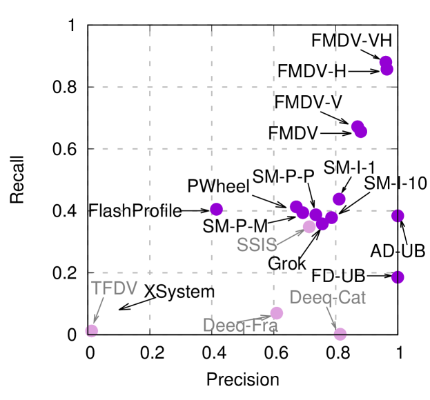
(a) Enterprise benchmark: Numbers reported using a subset of 571 cases where syntactic patterns exist.

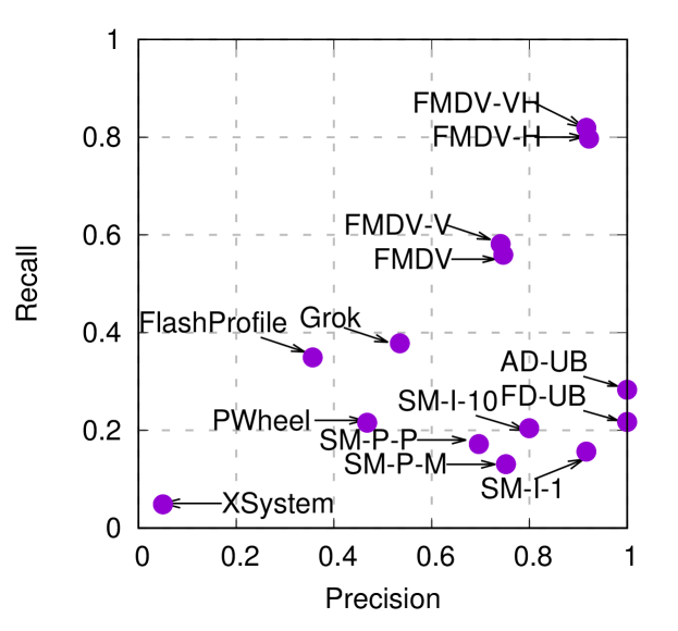
(b) Government benchmark: Numbers reported using a subset of 359 cases where syntactic patterns exist.

Figure 10. Recall vs. Precision comparisons of all methods, on Enterprise and Government benchmarks.

Evaluation Method	precision	recall
Programmatic evaluation	0.961	0.880
Hand curated ground-truth	0.963	0.915

Table 2. Quality results on $\mathbf{B_{E}}$, using programmatic evaluation vs. manually-cleaned ground-truth.

For all comparisons in Figure 10 discussed above, we perform statistical tests using the F-scores between FMDV-VH and all other methods on 1000 columns (where the null-hypothesis being the F-score of FMDV-VH is no better than a given baseline). We report that the $p$-values of all comparisons range from 0.001 to 0.007 (substantially smaller than the $p<0.05$ level), indicating that we should reject the null-hypothesis and the observed advantages are likely significant.

Manually-labeled ground-truth. While our programmatic evaluation provides a good proxy of the ground-truth without needing any labeling effort, we also perform a manual evaluation to verify the validity of the programmatic evaluation.

Specifically, we manually label the ground-truth validation patterns for 1000 test cases in $\mathbf{B_{E}}$, and perform two types of adjustments: (1) To accurately report precision, we manually remove values in the test-set of each column that should not belong to the column (e.g., occasionally column-headers are parsed incorrectly as data values), to ensure that we do not unfairly punish methods that identify correct patterns; and (2) To accurately report recall, we identify ground-truth patterns of each test query column, so that in recall evaluation if another column is drawn from the same domain with the identical pattern, we do not count it as a recall-loss.

We note that both adjustments improve the precision/recall, because our programmatic evaluation under-estimates the true precision/recall. Table 2 compares the quality results using programmatic evaluation and manual ground-truth, which confirms the validity of the programmatic evaluation.

Figure 11 shows a case-by-case analysis of F1 results on $\mathbf{B_{E}}$ with competitive methods, using 100 randomly sampled cases, sorted by their results on FMDV-VH to make comparison easy. We can see that FMDV dominates other methods. An error-analysis on the failed cases shows that these are mainly attributable to advanced pattern-constructs such as flexibly-formatted URLs, and unions of distinct patterns, which are not supported by our current profiler.

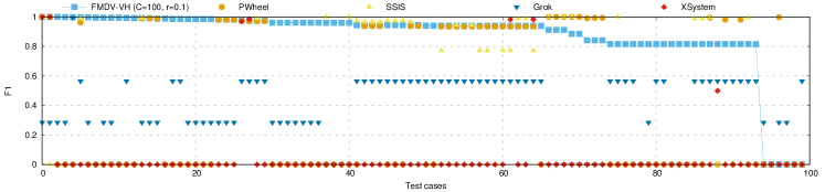
Figure 11. Case-by-case results reported using F-1 scores, on 100 randomly sampled cases.

Sensitivity. Figure 12 shows a detailed sensitivity analysis for all FMDV variants using average precision/recall. Figure 12(a) shows the result with a varying FRP target $r$, from the most strict 0 to a more lax 0.1. As we can see, $r$ values directly translate to a precision/recall trade-off and is an effective knob for different precision targets. For the proposed FMDV-VH variant, its performance is not sensitive for $r\geq 0.02$.

Figure 12(b) shows the effect of varying the coverage target $m$ from 0 to 100. We see that the precision/recall of our algorithms is not sensitive to $m$ in most cases, because the test columns we sample randomly are likely to have popular patterns matching thousands of columns. We recommend using a large $m$ (e.g., at least 100) to ensure confident domain inference.

Figure 12(c) shows the impact of varying $\tau$, which is the max number of tokens in a column for it to be indexed (Section 2.4). As can be seen from the figure, algorithms using vertical-cuts (FMDV-V and FMDV-VH) are insensitive to smaller $\tau$, while algorithms without vertical-cuts (FMDV and FMDV-H) suffer substantial recall loss with a small $\tau=8$, which shows the benefit of using vertical-cuts. We recommend using FMDV-VH with a small $\tau$ (e.g., 8), which is efficient and inexpensive to run.

Figure 12(d) shows the sensitivity to $\theta$. We can see that the algorithm is not sensitive to $\theta$, as long as it is not too small.

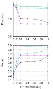
(a) Sensitivity to FPR threshold ($r$)

(b) Sensitivity to Coverage ($m$)

(c) Sensitivity to token-limit ($\tau$)

(d) Sensitivity of FMDV-H to ($\theta$)

Figure 12. Sensitivity analysis of FMDV algorithms on the Enterprise benchmark.

Pattern analysis. Because our offline index enumerates all possible patterns that can be generated from $\mathbf{T}$, it provides a unique opportunity to understand: (1) all common domains in $\mathbf{T}$ independent of query-columns, defined as patterns with high coverage and low FPR; and (2) the characteristics of all candidate patterns generated from $\mathbf{T}$.

For (1) we inspect the “head” patterns in the index file, e.g. patterns matching over 10K columns and with low FPR. This indeed reveals many common “domains” of interest in this data lake, some examples of which are shown in Figure 3. We note that identifying data domains in proprietary formats have applications beyond data validation (e.g., in enterprise data search), and is an interesting area for future research.

For (2), we show an analysis of all patterns in $\mathbf{T}$ using the index in Figure 13. Figure 13(a) shows the frequency of patterns by token-length (each <num>, <letter>, etc. is a token). We can see that the patterns are fairly evenly distributed, where patterns with 5-7 token are the most common. Figure 13(b) shows the frequency of all distinct candidate patterns. We observe a power-law-like distribution – while the “head” patterns are likely useful domain patterns, the vast majority have low coverage that are either generalized too narrowly or are not common domains.

(a) Pattern distr. by #-of-tokens

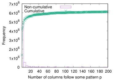
(b) Pattern distr. by frequency

Figure 13. Distribution of patterns in the offline index.

Efficiency. Figure 14 shows the average latency (in milliseconds) to process one query column $C$ in our benchmark. We emphasize that low latency is critical for human-in-the-loop scenarios (e.g., TFDV), where users are expected to verify suggested constraints.

On the right of the figure, we can see the average latency for PWheel, FalshProfile, and XSystem, respectively (we use authors’ original implementations for the last two methods (FlashProfileCode, ; xsystem-code, )). It can be seen that these existing pattern-profiling techniques all require on average 6-7 seconds per column. Given that tables often have tens of columns, the end-to-end latency can be slow.

In comparison, we observe that despite using a more involved algorithm and a large corpus $\mathbf{T}$, all FMDV variants are two orders of magnitude faster, where the most expensive FMDV-VH takes only 0.082 seconds per column. This demonstrates the benefit of the offline indexing step in Section 2.4, which distills $\mathbf{T}$ (in terabytes) down to a small index with summary statistics (with less than one gigabyte), and pushes expensive reasoning to offline, allowing for fast online response time. As an additional reference point, if we do not use offline indexes, the “FMDV (no-index)” method has to scan $\mathbf{T}$ for each query and is many orders of magnitude slower.

For the offline indexing step, we report that the end-to-end latency of our job (on a cluster with 10 virtual-nodes) ranges from around 1 hour (with $\tau=8$), to around 3 hours (with $\tau=13$). We believe this shows that our algorithm is viable even on small-scale clusters, despite using a large number of patterns.

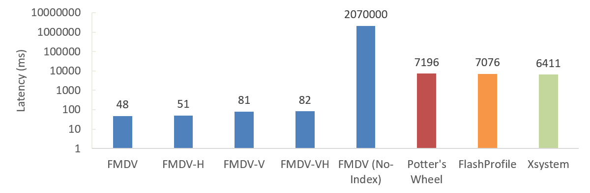
Figure 14. Latency in milliseconds (per query column).

User study. To evaluate the human benefit of suggesting data-validation patterns, we perform a user study by recruiting 5 programmers (all with at least 5 years of programming experience), to write data-validation patterns for 20 sampled test columns in benchmark $\mathbf{B_{E}}$. This corresponds to the scenario of developers manually writing patterns without using the proposed algorithm.

Programmer	avg-time (sec)	avg-precision	avg-recall
#1	145	0.65	0.638
#2	123	0.45	0.431
#3	84	0.3	0.266
FMDV-VH	0.08	1.0	0.978

Table 3. User study comparing 3 developers with FMDV-VH on 20 test columns, by time spent and pattern quality.

We report that 2 out of the 5 users fail completely on the task (their regex are either ill-formed or fail to match given examples). Table 3 shows the results for the remaining 3 users. We observe that on average, they spend 117 seconds to write a regex for one test column (for it often requires many trials-and-errors). This is in sharp contrast to 0.08 seconds required by our algorithm. Programmers’ average precision is 0.47, also substantially lower than the algorithm’s precision of 1.0 on hold-out test data.

Case studies using Kaggle. In order to use publicly available data sets to assess the benefits of data validation against schema-drift, we conduct a case study using 11 tasks sampled from Kaggle (kaggle, ), where each task has at least 2 string-valued categorical attributes. These 11 tasks include 7 for classification: Titanic, AirBnb, BNPParibas, RedHat, SFCrime, WestNile, WalmartTrips; and 4 for regression: HousePrice, HomeDepot, Caterpillar, and WalmartSales.

To simulate schema-drift (breck2019data, ; polyzotis2017data, ; schelter2018automating, ), for each Kaggle task, we keep the training data unchanged, but swap the position of the categorical attributes in the testing data (e.g., if a data set has two attributes date and time at column-position 1 and 2, respectively, after simulated schema-drift the two attributes will be at column-position 2 and 1, respectively). This creates a small schema-mismatch between training/testing data that is hard to detect but can be common in practice like explained in (breck2019data, ; polyzotis2017data, ).

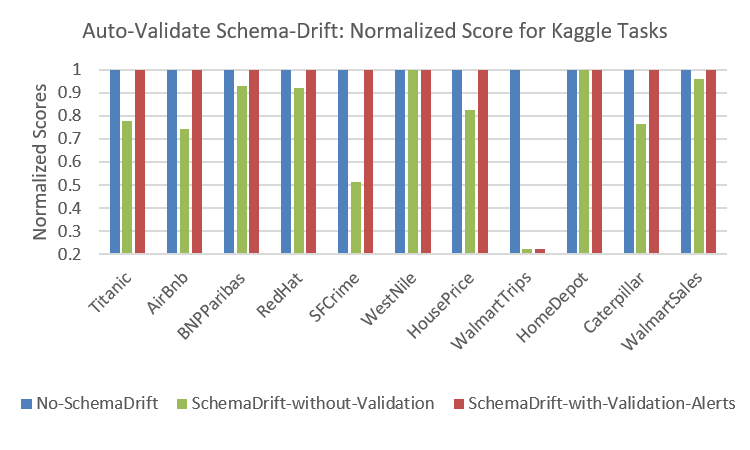
Figure 15. Impact of schema-shift on Kaggle tasks, with and without data-validation. FMDV detects schema-drift in 8 out of 11 cases.

Figure 15 shows the quality results with and without validation on these Kaggle tasks. For all tasks, we use a popular GBDT method called XGBoost (xgboost, ) with default parameters. We report R2 for regression tasks and average-precision for classification tasks.

The left (blue) bar of each task, labeled as No-SchemaDrift, shows the prediction-quality scores, on the original datasets and without schema-drift. We normalize these scores as 100%. The middle (green) bar, SchemaDrift-without-Validation, shows the quality scores with schema-drift, measured relative to the original quality scores. We observe a drop up to 78% (WalmartTrips) in normalized scores. Lastly, the right (red) bar, SchemaDrift-with-Validation shows the quality when data-validation is used, which correctly detect schema-drift in 8 out of 11 tasks (all except WestNile, HomeDepot and WalmartTrips, with no false-positives). Addressing such validation alerts would significantly boost the resulting quality scores. s While it is generally known that schema-drift hurts ML quality (breck2019data, ; TFDV, ), our analysis quantifies its impact on publicly available data and confirms the importance of data-validation.

6. Related Works

Data Validation. Notable recent efforts on data validation include Google’s TensorFlow Data Validation (TFDV) (breck2019data, ; TFDV, ) and Amazon’s Deequ (Deequ, ; schelter2018automating, ). These offerings allow developers to write declarative data quality constraints to describe how “normal” data should look like, which are described in detail in the introduction.

Error Detection. There is an influential line of work on error-detection, including methods that focus on multi-column dependencies, such as FDs and denial constraints (e.g., (berti2018discovery, ; chiang2008discovering, ; chu2013, ; dasu2002mining, ; golab2010data, ; ilyas2004cords, ; kivinen1995approximate, ; yancoded, )), where most techniques would require some amount of human supervision (e.g., manually specified/verified constraints). Auto-Validate is unsupervised and focuses on single-column constraints, which naturally complements existing work.

Recent approaches propose learning-based error-detection methods (e.g., (heidari2019holodetect, ; huang2018auto, ; liu2020picket, ; mahdavi2019raha, ; qahtan2019anmat, ; yan2020scoded, ; wang2019uni, )), some of which are unsupervised (huang2018auto, ; liu2020picket, ; wang2019uni, ) and similar in spirit to Auto-Validate.

Pattern Profiling. There is also a long line of work on pattern profiling, including pioneering methods such as Potter’s wheel (raman2001potter, ) that leverages the MDL principle, and other related techniques (ilyas2018extracting, ; fisher2005pads, ; fisher2008dirt, ; naumann2014data, ). While both data validation and profiling produce patterns, data profiling only aims to produce patterns to “cover” given values in a column $C$, without considering valid values from the same domain but not in $C$, and is thus prone to false-positives when used for data validation (for data that arrive in the future).

Other forms to validation. While pattern-based validation is a natural fit for machine-generated data; alternative forms of validation logic can be more suited for other types of data. For example, for natural-language data drawn from a fixed vocabulary (e.g., countries or airport-codes), dictionary-based validation learned from examples (e.g., set expansion (he2011seisa, ; pantel2009web, ; wang2007language, )) is applicable. For complex types, semantic-type validation (hulsebos2019sherlock, ; yan2018synthesizing, ; zhang2019sato, ) is also a suitable choice.

7. Conclusions and Future Work

Observing the need to automate data-validation in production pipelines, we propose a corpus-driven approach to inferring single-column constraints that can be used to auto=validate string-valued data. Possible directions of future work include extending beyond “machine-generated data” to consider natural-language-like data, and extending the same validation principle also to numeric data.

References

- [1] Amazon Deequ Library for Data Validation. https://github.com/awslabs/deequ.
- [2] AWS Glue custom classifers. https://docs.aws.amazon.com/glue/latest/dg/custom-classifier.html.
- [3] Azure ML: Data Pipelines. https://docs.microsoft.com/en-us/azure/machine-learning/concept-ml-pipelines.
- [4] Azure Purview for data governance. https://azure.microsoft.com/en-us/services/purview/.
- [5] Bing entity search. https://azure.microsoft.com/en-us/services/cognitive-services/bing-entity-search-api/.
- [6] Data Crawler for NationalArchives.gov.uk. https://github.com/alex-bogatu/DataSpiders.
- [7] FlashProfile package. https://www.nuget.org/packages/Microsoft.ProgramSynthesis.Extraction.Text/.
- [8] Google TensorFlow Data Validation. https://www.tensorflow.org/tfx/guide/tfdv.
- [9] Grok Patterns. https://github.com/elastic/elasticsearch/blob/master/libs/grok/src/main/resources/patterns/grok-patterns.
- [10] Informatica Rev. https://www.informatica.com/products/data-quality/rev.html.
- [11] Kaggle. https://www.kaggle.com/.
- [12] Power BI: Data Flow. https://docs.microsoft.com/en-us/power-bi/transform-model/service-dataflows-create-use.
- [13] SSIS: Data Profiling. https://docs.microsoft.com/en-us/sql/integration-services/control-flow/data-profiling-task?view=sql-server-ver15.
- [14] Tableau: Flow. https://help.tableau.com/current/prep/en-us/prep_build_flow.htm.
- [15] Tableau: Flow. https://aws.amazon.com/blogs/big-data/simplify-data-pipelines-with-aws-glue-automatic-code-generation-and-workflows/.
- [16] XGBoost. https://xgboost.readthedocs.io/en/latest/.
- [17] XSystem Code. https://bitbucket.org/andrewiilyas/xsystem-old/src/outlier-detection/.
- [18] A. Agresti et al. A survey of exact inference for contingency tables. Statistical science, 7(1):131–153, 1992.
- [19] L. Berti-Equille, H. Harmouch, F. Naumann, N. Novelli, and S. Thirumuruganathan. Discovery of genuine functional dependencies from relational data with missing values. VLDB, 2018.
- [20] A. Bogatu, A. A. Fernandes, N. W. Paton, and N. Konstantinou. Dataset discovery in data lakes. In 2020 IEEE 36th International Conference on Data Engineering (ICDE), pages 709–720. IEEE, 2020.
- [21] E. Breck, N. Polyzotis, S. Roy, S. Whang, and M. Zinkevich. Data validation for machine learning. In Conference on Systems and Machine Learning (SysML). https://www. sysml. cc/doc/2019/167. pdf, 2019.
- [22] H. Carrillo and D. Lipman. The multiple sequence alignment problem in biology. SIAM journal on applied mathematics, 48(5):1073–1082, 1988.
- [23] R. Chaiken, B. Jenkins, P.-Å. Larson, B. Ramsey, D. Shakib, S. Weaver, and J. Zhou. Scope: easy and efficient parallel processing of massive data sets. Proceedings of the VLDB Endowment, 1(2):1265–1276, 2008.
- [24] G. Chen, K. Yang, L. Chen, Y. Gao, B. Zheng, and C. Chen. Metric similarity joins using mapreduce. IEEE Transactions on Knowledge and Data Engineering, 29(3):656–669, 2016.
- [25] F. Chiang and R. J. Miller. Discovering data quality rules. VLDB, 1(1), 2008.
- [26] X. Chu, I. F. Ilyas, and P. Papotti. Discovering denial constraints. VLDB, 6(13), 2013.
- [27] T. H. Cormen, C. E. Leiserson, R. L. Rivest, and C. Stein. Introduction to algorithms. MIT press, 2009.
- [28] A. Das Sarma, Y. He, and S. Chaudhuri. Clusterjoin: A similarity joins framework using map-reduce. Proceedings of the VLDB Endowment, 7(12):1059–1070, 2014.
- [29] T. Dasu, T. Johnson, S. Muthukrishnan, and V. Shkapenyuk. Mining database structure; or, how to build a data quality browser. In SIGMOD, 2002.
- [30] U. Dayal, M. Castellanos, A. Simitsis, and K. Wilkinson. Data integration flows for business intelligence. In Proceedings of the 12th International Conference on Extending Database Technology: Advances in Database Technology, pages 1–11, 2009.
- [31] K. Fisher and R. Gruber. Pads: a domain-specific language for processing ad hoc data. ACM Sigplan Notices, 40(6):295–304, 2005.
- [32] K. Fisher, D. Walker, K. Q. Zhu, and P. White. From dirt to shovels: fully automatic tool generation from ad hoc data. ACM SIGPLAN Notices, 43(1):421–434, 2008.
- [33] L. Golab, H. Karloff, F. Korn, and D. Srivastava. Data auditor: Exploring data quality and semantics using pattern tableaux. VLDB, 3(1-2), 2010.
- [34] Y. He, J. Song, Y. Wang, S. Chaudhuri, V. Anil, B. Lassiter, Y. Goland, and G. Malhotra. Auto-tag: Tagging-data-by-example in data lakes using pre-training and inferred domain patterns.
- [35] Y. He and D. Xin. Seisa: set expansion by iterative similarity aggregation. In Proceedings of the 20th international conference on World wide web, pages 427–436, 2011.
- [36] A. Heidari, J. McGrath, I. F. Ilyas, and T. Rekatsinas. Holodetect: Few-shot learning for error detection. In Proceedings of the 2019 International Conference on Management of Data, pages 829–846, 2019.
- [37] Z. Huang and Y. He. Auto-Detect: Data-Driven Error Detection in Tables. In SIGMOD, 2018.
- [38] M. Hulsebos, K. Hu, M. Bakker, E. Zgraggen, A. Satyanarayan, T. Kraska, Ç. Demiralp, and C. Hidalgo. Sherlock: A deep learning approach to semantic data type detection. In Proceedings of the 25th ACM SIGKDD International Conference on Knowledge Discovery & Data Mining, pages 1500–1508, 2019.
- [39] N. Hynes, D. Sculley, and M. Terry. The data linter: Lightweight, automated sanity checking for ml data sets. In NIPS MLSys Workshop, 2017.
- [40] A. Ilyas, J. M. da Trindade, R. C. Fernandez, and S. Madden. Extracting syntactical patterns from databases. In 2018 IEEE 34th International Conference on Data Engineering (ICDE), pages 41–52. IEEE, 2018.
- [41] I. F. Ilyas, V. Markl, P. Haas, P. Brown, and A. Aboulnaga. Cords: automatic discovery of correlations and soft functional dependencies. In SIGMOD, 2004.
- [42] W. Just. Computational complexity of multiple sequence alignment with sp-score. Journal of computational biology, 8(6):615–623, 2001.
- [43] G. K. Kanji. 100 statistical tests. Sage, 2006.
- [44] R. M. Karp and A. Wigderson. A fast parallel algorithm for the maximal independent set problem. Journal of the ACM (JACM), 32(4):762–773, 1985.
- [45] J. Kivinen and H. Mannila. Approximate inference of functional dependencies from relations. Theoretical Computer Science, 149(1), 1995.
- [46] Z. Liu, Z. Zhou, and T. Rekatsinas. Picket: Self-supervised data diagnostics for ml pipelines. arXiv preprint arXiv:2006.04730, 2020.
- [47] M. Mahdavi, Z. Abedjan, R. Castro Fernandez, S. Madden, M. Ouzzani, M. Stonebraker, and N. Tang. Raha: A configuration-free error detection system. In Proceedings of the 2019 International Conference on Management of Data, pages 865–882, 2019.
- [48] F. Naumann. Data profiling revisited. ACM SIGMOD Record, 42(4):40–49, 2014.
- [49] S. Padhi, P. Jain, D. Perelman, O. Polozov, S. Gulwani, and T. Millstein. Flashprofile: a framework for synthesizing data profiles. Proceedings of the ACM on Programming Languages, 2(OOPSLA):1–28, 2018.
- [50] P. Pantel, E. Crestan, A. Borkovsky, A.-M. Popescu, and V. Vyas. Web-scale distributional similarity and entity set expansion. In Proceedings of the 2009 Conference on Empirical Methods in Natural Language Processing, pages 938–947, 2009.
- [51] T. Papenbrock and F. Naumann. A hybrid approach to functional dependency discovery. In Proceedings of the 2016 International Conference on Management of Data, pages 821–833, 2016.
- [52] H. Patel, A. Jindal, and C. Szyperski. Big data processing at microsoft: Hyper scale, massive complexity, and minimal cost. In Proceedings of the ACM Symposium on Cloud Computing, pages 490–490, 2019.
- [53] N. Polyzotis, S. Roy, S. E. Whang, and M. Zinkevich. Data management challenges in production machine learning. In Proceedings of the 2017 ACM International Conference on Management of Data, pages 1723–1726, 2017.
- [54] A. Qahtan, N. Tang, M. Ouzzani, Y. Cao, and M. Stonebraker. Anmat: automatic knowledge discovery and error detection through pattern functional dependencies. In Proceedings of the 2019 International Conference on Management of Data, pages 1977–1980, 2019.
- [55] E. Rahm and P. A. Bernstein. A survey of approaches to automatic schema matching. the VLDB Journal, 10(4):334–350, 2001.
- [56] E. Rahm and H. H. Do. Data cleaning: Problems and current approaches. IEEE Data Eng. Bull., 23(4):3–13, 2000.
- [57] V. Raman and J. M. Hellerstein. Potter’s wheel: An interactive data cleaning system. In VLDB, volume 1, 2001.
- [58] S. Schelter, F. Biessmann, D. Lange, T. Rukat, P. Schmidt, S. Seufert, P. Brunelle, and A. Taptunov. Unit testing data with deequ. In Proceedings of the 2019 International Conference on Management of Data, pages 1993–1996, 2019.
- [59] S. Schelter, S. Grafberger, P. Schmidt, T. Rukat, M. Kiessling, A. Taptunov, F. Biessmann, and D. Lange. Differential data quality verification on partitioned data. In 2019 IEEE 35th International Conference on Data Engineering (ICDE), pages 1940–1945. IEEE, 2019.
- [60] S. Schelter, D. Lange, P. Schmidt, M. Celikel, F. Biessmann, and A. Grafberger. Automating large-scale data quality verification. Proceedings of the VLDB Endowment, 11(12):1781–1794, 2018.
- [61] M. Stonebraker and I. F. Ilyas. Data integration: The current status and the way forward. IEEE Data Eng. Bull., 41(2):3–9, 2018.
- [62] A. Swami, S. Vasudevan, and J. Huyn. Data sentinel: A declarative production-scale data validation platform. In 2020 IEEE 36th International Conference on Data Engineering (ICDE), pages 1579–1590. IEEE, 2020.
- [63] P. Vassiliadis and A. Simitsis. Near real time etl. In New trends in data warehousing and data analysis, pages 1–31. Springer, 2009.
- [64] P. Wang and Y. He. Uni-detect: A unified approach to automated error detection in tables. In Proceedings of the 2019 International Conference on Management of Data, pages 811–828, 2019.
- [65] R. C. Wang and W. W. Cohen. Language-independent set expansion of named entities using the web. In Seventh IEEE international conference on data mining (ICDM 2007), pages 342–350. IEEE, 2007.
- [66] C. Yan and Y. He. Auto-Type: Synthesizing type-detection logic for rich semantic data types using open-source code. In Proceedings of the 2018 International Conference on Management of Data. ACM, 2018.
- [67] J. N. Yan, O. Schulte, J. Wang, and R. Cheng. Coded: Column-oriented data error detection with statistical constraints.
- [68] J. N. Yan, O. Schulte, M. Zhang, J. Wang, and R. Cheng. Scoded: Statistical constraint oriented data error detection. In Proceedings of the 2020 ACM SIGMOD International Conference on Management of Data, pages 845–860, 2020.
- [69] D. Zhang, Y. Suhara, J. Li, M. Hulsebos, Ç. Demiralp, and W.-C. Tan. Sato: Contextual semantic type detection in tables. arXiv preprint arXiv:1911.06311, 2019.
- [70] J. Zhou, N. Bruno, M.-C. Wu, P.-A. Larson, R. Chaiken, and D. Shakib. Scope: parallel databases meet mapreduce. The VLDB Journal, 21(5):611–636, 2012.