April 2021

ABSTRACT

Samples of dynamic or time-varying networks and other random object data such as time-varying probability distributions are increasingly encountered in modern data analysis. Common methods for time-varying data such as functional data analysis are infeasible when observations are time courses of networks or other complex non-Euclidean random objects that are elements of general metric spaces. In such spaces, only pairwise distances between the data objects are available and a strong limitation is that one cannot carry out arithmetic operations due to the lack of an algebraic structure. We combat this complexity by a generalized notion of mean trajectory taking values in the object space. For this, we adopt pointwise Fréchet means and then construct pointwise distance trajectories between the individual time courses and the estimated Fréchet  mean trajectory, thus representing the time-varying objects and networks by functional data. Functional principal component analysis of these distance trajectories can reveal interesting features of dynamic networks and object time courses and is useful for downstream analysis. Our approach also makes it possible to study the empirical dynamics of time-varying objects, including dynamic regression to the mean or explosive behavior over time. We demonstrate desirable asymptotic properties of sample based estimators for suitable population targets under mild assumptions. The utility of the proposed methodology is illustrated with dynamic networks, time-varying distribution data and longitudinal growth data.

KEY WORDS: Empirical dynamics; Fréchet mean trajectory; Functional data analysis; Metric space; Object time courses; Time-varying distributions; Time-varying networks.

1. INTRODUCTION

Longitudinal or time-varying data consist of repeated observations for each subject at different time points, where one has such observations for a sample of independent subjects. Tools for analyzing both univariate and multivariate longitudinal data have been well studied (Fitzmaurice et al. 2008; Verbeke et al. 2014; Fieuws and Verbeke 2006; Berrendero et al. 2011; Zhou et al. 2008; Xiang et al. 2013). When such data are scalar or Euclidean vectors and densely measured in time, they can be analyzed as functional data (Rice 2004; Guo 2004; Yang et al. 2007), where functional data analysis provides a flexible nonparametric framework with a well established toolbox. This popular methodology requires a vector space structure of the observed data and is therefore restricted to the case where the measurements at each fixed time are scalars or Euclidean vectors (Ramsay and Silverman 2005; Ferraty et al. 2007; Horvath and Kokoszka 2012; Hsing and Eubank 2015; Wang et al. 2016).

Time-varying object data are becoming more frequent and are encountered in time-varying social networks, traffic networks that change over time, brain networks between hubs that evolve with age, and many other settings (Nie et al. 2017). While such data have similarities with densely measured functional data, the observations at each time point are neither scalars nor vectors as in classical functional data analysis, but instead take values in a general metric space. A major challenge is that in such spaces typical vector space operations such as addition, scalar multiplication or inner products are not defined. In general metric spaces, the only information available are pairwise distances between the random objects at each observation time, and therefore the tools of functional and longitudinal data analysis are not directly applicable. We develop here a simple method that bypasses these challenges by focusing on distances as outcomes.

Models for time courses of non-Euclidean objects have been developed for shape evolution as a continuous diffeomorphic deformation of a baseline shape over time (Durrleman et al. 2013) and for the analysis of longitudinal data taking values in smooth Riemannian manifolds (Schiratti et al. 2015; Muralidharan and Fletcher 2012; Anirudh et al. 2017; Dai and Müller 2018). These methods exploit the local Euclidean nature of Riemannian manifolds but are not applicable for the analysis of data objects in more general metric spaces that do not have a natural Riemannian geometry. For this general case, a fairly complex and challenging methodology has been developed in Dubey and Müller (2019b). We propose here a more straightforward approach that allows us to cut through the challenges posed by longitudinal metric space valued data by focusing on the distance of time-varying random objects from the mean trajectory and thereby reducing such data to classical functional data.

A related topic is the analysis of longitudinal functional data, where the observations at each time point are functional rather than scalar. For this scenario, previous approaches (Chen et al. 2017) have utilized a tensor product representation of the function-valued stochastic process, an approach for which an underlying Hilbert space is essential and that cannot be directly extended to non-Hilbertian data that we consider here. While complex longitudinal network data have been extensively studied (Snijders 2005; Huisman and Snijders 2003; Kossinets and Watts 2006), these efforts have been directed specifically towards studying dynamics of evolution of a single network with a variety of network effects and are not applicable to the study of the dynamics of a sample of network trajectories or longitudinal trajectories of other general data objects.

Our goal in this paper is to provide a straightforward methodology for analyzing functional object data, i.e., time-varying random objects including dynamic networks that live in general metric spaces. Converting such data to functional data makes it possible to tap the rich existing toolbox of functional data analysis, while imposing not more than mild entropy conditions on the underlying object space. We assume that the data objects take values in a totally bounded metric space and that the random object trajectories are fully observed. Since many dynamic developments of interest can be expressed in terms of departure of an observed dynamic process from a baseline process, we use a suitably defined mean trajectory that takes values in the object space as baseline.

For metric space valued data, Fréchet developed a generalization of the usual population and sample means (Fréchet 1948), which then gives rise to a generalization of the notion of variance for object data, quantifying the variation of such data around the Fréchet mean. It is thus natural to take as mean trajectory of the object functional data the trajectory consisting of the pointwise Fréchet means, obtained at each time point. In order to study individual deviations of each time course from this mean trajectory, we first construct squared distance trajectories of the individual object functions from the Fréchet mean trajectory. These squared distance trajectories, which we refer to as subject specific Fréchet variance trajectories, are scalar valued functional data in contrast to the object trajectories themselves, and therefore can be subjected to the standard tools that have been developed for functional data analysis, including the highly successful functional principal component analysis (Kleffe 1973; Hall and Hosseini-Nasab 2006; Li and Guan 2014; Chen and Lei 2015; Lin et al. 2016).

One major obstacle in working with subject specific Fréchet variance trajectories, which makes it difficult to directly apply functional data methods, is that the population Fréchet mean trajectory is not known and has to be estimated from the data. The squared distance trajectories which are used for the analysis are then the squared distances of the individual time courses from the sample Fréchet mean trajectory. This makes the subject-specific Fréchet variance trajectories dependent and so they cannot be treated as independent observations of random trajectories, which is essential for the application of the usual functional data analysis tools. By imposing mild assumptions on the entropy of the underlying metric space and on the continuity of the random object trajectories, we are able to overcome this problem and to establish desirable asymptotic properties of the estimators of suitably defined population targets, including rates of convergence.

As we demonstrate in various applications, functional principal component analysis of the subject-specific Fréchet variance trajectories can lead to interesting insights regarding the behavior of the object trajectories. Clustering is often a useful first step for exploratory data analysis, aiming to identify homogeneous subgroups and patterns that have some meaningful interpretation for the researcher. Functional data are inherently infinite-dimensional and a probability density generally does not exist, which contributes to the challenge of clustering functional data (Chiou and Li 2007; Jacques and Preda 2014; Tarpey and Kinateder 2003; Ciollaro et al. 2016; Suarez and Ghosal 2016). An additional difficulty arises when the observations at each time point are not in a vector space. Eigenfunctions of the covariance surface of the Fréchet variance functions can nevertheless pinpoint predominant modes of variation of the individual Fréchet variance trajectories around the average Fréchet variance trajectory and projection scores of the subject-specific Fréchet variance trajectories along these eigenfunctions can reveal inherent clustering within the object trajectories, as we will illustrate in our data applications.

Identifying extremes and potential outliers is challenging for functional data because the observations at a given time point itself may not be unusual in their value but the overall shape of an observed curve may be very different from that of the bulk of curves. Object time courses are even more intractable. Statistical data depth is a concept introduced to measure the “centrality” or the “outlyingness” of an observation within a given data set or an underlying distribution and this concept has been extended to functional data in recent years (López-Pintado and Romo 2009; Nagy et al. 2017; Nagy and Ferraty 2019; Agostinelli 2018), where it has been used widely for the detection of extremes and potential outliers in functional data (Ren et al. 2017; Febrero et al. 2008; Arribas-Gil and Romo 2014; Romano and Mateu 2013).

An important aspect of our analysis is that conclusions about the behavior of object time courses are drawn based on their squared distances from the Fréchet mean trajectory. The Fréchet mean trajectory is a representative for the most central point for a sample of object functions and the subject specific Fréchet variance time courses carry information about the deviations of individual trajectories from the ‘central’ trajectory, which leads to a central-outward ordering for the sample trajectories. We show that principal component projection scores of the subject specific Fréchet variance time courses along eigenfunctions are useful for visualization of the longitudinal object data and also for the detection of extremes. Another aspect of interest is the dynamics of the evolving object trajectories, especially whether they tend to move closer to the mean function as time progresses, so that a far away trajectory will tend to be drawn towards the center (centripetality) or will move further away from the center (centrifugality), as time progresses.

The paper is organized as follows: In Section 2, we introduce our framework and define the population targets and the corresponding sample based estimators. The theoretical properties of the estimators are established in Section 3. This is followed by data illustrations in Section 4, where we apply the proposed method for the longitudinal network generated by the Chicago Divvy bike data for the years 2014 to 2017, for the longitudinal annual fertility data for 26 countries over 34 calendar years from 1976 to 2009 and for time varying shape data using the Zürich longitudinal growth study. We also demonstrate the proposed quantification of the underlying dynamics of the observed processes. Simulation results for a sample of time-varying networks are presented in Section 5, followed by a discussion in Section 6. Auxiliary results and proofs can be found in the online supplement.

2. PRELIMINARIES AND ESTIMATION

We consider an object space $(\Omega,d)$ that is a totally separable bounded metric space and an $\Omega$-valued stochastic process $\{X(t)\}_{t\in[0,1]}$, alternatively referred to as $X$ for ease of notation, and assume that one observes a sample of random object trajectories $X_{1},X_{2},\dots,X_{n}$, which are independently and identically distributed copies of the random process $X$ with respect to an underlying probability measure $P$. For each subject-specific trajectory $X_{i}$, we aim to quantify its deviation from a baseline object function, which can be thought of as the mean or typical population trajectory. A natural baseline for real-valued functional data is the mean function. For more general general object-valued trajectories, we propose to use the population Fréchet mean trajectory as baseline function, defined as the pointwise Fréchet mean function, where for given $t\in[0,1]$, the population and sample Fréchet mean trajectories at $t$ are defined as

$$\mu(t)=\operatorname*{argmin}_{\omega\in\Omega}E\left(d^{2}(X(t),\omega)\right),\quad\hat{\mu}(t)=\operatorname*{argmin}_{\omega\in\Omega}\frac{1}{n}\sum_{i=1}^{n}d^{2}(X_{i}(t),\omega),$$ (1)

respectively. Here we assume that for all $t\in[0,1]$ these minimizers exist and are unique. While the existence and uniqueness of Fréchet means is not guaranteed in general spaces (Bhattacharya and Patrangenaru 2003), for the case of Hadamard spaces, which have globally nonpositive curvature, Fréchet means as defined in equation (1) exist and are unique (Sturm 2003). For positively curved spaces see Ahidar-Coutrix et al. (2020).

The target functions for our analysis then ideally would be the functions

$$V^{\ast}_{i}(t)=d^{2}(X_{i}(t),\mu(t)),\,\,t\in[0,1],$$ (2)

which correspond to the pointwise squared distance functions of the subject trajectories $X_{i}$ from the population Fréchet mean function $\mu=\mu(t)$ for the subject trajectories $X_{i}$. These can be characterized as the subject-specific oracle Fréchet variance trajectories. They are however unavailable, since the population Fréchet mean trajectory $\mu$ is unknown and needs to be estimated from the data. From (2) one obtains the data-based version

$$V_{i}(t)=d^{2}(X_{i}(t),\hat{\mu}(t)),\,t\in[0,1],$$ (3)

where $\hat{\mu}$ is as in (1) and we refer to the $V_{i}=V_{i}(t)$ as the sample Fréchet variance trajectories and write $V(t)=d^{2}(X(t),\hat{\mu}(t))$ for the generic version. Since they all depend on $\hat{\mu}(t)$, the sample Fréchet variance trajectories are dependent and cannot be treated as independent realizations of a stochastic process, which is the standard framework for functional data analysis, thus posing a challenge for theory.

Suppose for the moment that we have available an i.i.d. sample of oracle Fréchet variance trajectories $V^{\ast}_{i}$, with generic version denoted by $V^{\ast}$. Then a typical dimension reduction step in Functional Data Analysis (FDA) is to apply Functional Principal Component Analysis (FPCA), which facilitates the conversion of the functional data $V^{\ast}_{i}$ to a countable sequence of uncorrelated random variables, the functional principal components (FPCs), where the sequence of FPCs is often truncated at a finite dimensional random vector to achieve dimension reduction. FPCA is based on using the eigenfunctions of the auto-covariance operator of the process $V^{\ast}$. This is an integral operator, a trace class and moreover compact Hilbert Schmidt operator (Hsing and Eubank 2015) that has the population Fréchet covariance surface $C$ as its kernel, where

$$C(s,t)=E\left(d^{2}(X(s),\mu(s))d^{2}(X(t),\mu(t))\right)-E\left(d^{2}(X(s),\mu(s))\right)E\left(d^{2}(X(t),\mu(t))\right).$$ (4)

The eigenvalues of the auto-covariance operator are nonnegative as the covariance surface is symmetric and nonnegative definite. By Mercer’s theorem,

$$C(s,t)=\sum_{j=1}^{\infty}\lambda_{j}\phi_{j}(s)\phi_{j}(t),\quad s,t\in[0,1],$$

with uniform convergence, where the $\lambda_{j}$ are the eigenvalues of the covariance operator, ordered in decreasing order, and $\phi_{j}(\cdot)$ are the corresponding orthonormal eigenfunctions.

This leads to the Karhunen-Loève expansion of the oracle Fréchet variance trajectories,

$$V^{\ast}_{i}(t)=\nu^{\ast}(t)+\sum_{j=1}^{\infty}B_{ij}\phi_{j}(t),$$ (5)

with $L^{2}$ convergence. Here $\nu^{\ast}$ is the mean function of the subjectwise Fréchet variance functions, $\nu^{\ast}(t)=E(d^{2}(X(t),\mu(t))),$ the population Fréchet variance function. The $B_{ij}$ are the FPCs, which are uncorrelated across $j$ with $E(B_{ij})=0$, ${\rm var}(B_{ij})=\lambda_{j}$ and $B_{ij}=\int(V^{\ast}_{i}(t)-\nu^{\ast}(t))\phi_{j}(t)dt.$ If $\mu$ is known, according to (4), the oracle estimator of the Fréchet covariance surface is

$$\tilde{C}(s,t)=\frac{1}{n}\sum_{i=1}^{n}V^{\ast}_{i}(s)V^{\ast}_{i}(t)-\frac{1}{n}\sum_{i=1}^{n}V^{\ast}_{i}(s)\,\,\frac{1}{n}\sum_{i=1}^{n}V^{\ast}_{i}(t).$$ (6)

Under mild assumptions on the functional trajectories $V_{i}^{*}$, standard asymptotic theory from functional data analysis shows that this estimator has desirable asymptotic properties and converges to the true covariance surface $C$ (4) (Hall and Hosseini-Nasab 2006).

As the population Fréchet mean function $\mu$ in reality is however unknown, we need to replace it by the sample based estimator $\hat{\mu}$ of the Fréchet covariance surface,

$$\hat{C}(s,t)=\frac{1}{n}\sum_{i=1}^{n}V_{i}(s)V_{i}(t)-\frac{1}{n}\sum_{i=1}^{n}V_{i}(s)\,\,\frac{1}{n}\sum_{i=1}^{n}V_{i}(t),$$ (7)

using the data-based distance processes $V_{i}(t)$ (3) that depend on estimates $\hat{\mu}$. We show in Section 3 that $\hat{C}$ is asymptotically close to the oracle estimator of the Fréchet covariance surface $\tilde{C}$ under mild regularity conditions on the metric space and the object functions and therefore has desirable asymptotic properties as an estimator of the population Fréchet covariance surface.

Estimates of eigenvalues and eigenfunctions are obtained as the empirical eigenvalues and eigenfunctions of the integral covariance operator with covariance kernel $\hat{C}$, and will be denoted by $\hat{\lambda}_{j}$ and $\hat{\phi_{j}}$, ordered in decreasing order of the eigenvalues. Eigenfunctions $\phi_{j}$ can be interpreted as coordinate directions, thereby providing the basis for principal modes of variation of the subject specific oracle Fréchet variance trajectories around the population Fréchet variance trajectory. Modes of variation (Castro et al. 1986; Lila and Aston 2019) are useful to quantify the departure of a random object trajectory from the Fréchet mean function. The eigenfunctions can be viewed as modes of outlyingness of the subject-specific trajectories. The estimates of the projection scores $B_{ij}$ of the $i^{th}$ oracle Fréchet variance trajectory on the $j^{th}$ eigenfunction are given by

$$\hat{B}_{ij}=\int_{0}^{1}\left(V_{i}(t)-\frac{1}{n}\sum_{k=1}^{n}V_{k}(t)\right)\hat{\phi}_{j}(t)dt.$$ (8)

We show in section 3. that under regularity assumptions, the $\hat{B}_{ij}$ are asymptotically close to the $B_{ij}$ in (5). These scores are useful for visualizing common traits in object trajectories and for detecting extremes, homogeneous subgroups or clusters in the data.

3. THEORY

We establish asymptotic properties of the empirical estimators of the population targets as described in section 2., assuming that the realizations of the object valued random process $X(t),\,\,t\in[0,1]$, have continuous sample paths almost surely and take values in a totally bounded metric space $(\Omega,d)$ and the following conditions are satisfied:

• The objects $\mu(s)$ and $\hat{\mu}(s)$ exist and are unique, the latter almost surely, for each $s\in[0,1]$. Additionally for any $\epsilon>0$,

  $$\inf_{s\in[0,1]}\inf_{\,\omega\in\Omega:\,d(\omega,\mu(s))>\epsilon}E(d^{2}(X(s),\omega))-E(d^{2}(X(s),\mu(s)))>0$$

  and there exists a $\tau=\tau(\epsilon)>0$ such that

  $$\lim_{n\rightarrow\infty}P\left(\inf_{s\in[0,1]}\inf_{\,\omega\in\Omega:\,d(\omega,\hat{\mu}(s))>\epsilon}\frac{1}{n}\sum_{l=1}^{n}\{d^{2}(X_{i}(s),\omega)-d^{2}(X_{i}(s),\hat{\mu}(s))\}\geq\tau(\epsilon)\right)=1.$$

• There exists $\rho>0,\ D>0$ and $\beta>1$ such that

  $$\inf_{s\in[0,1]}\inf_{\,\omega\in\Omega:\,d(\omega,\mu(s))<\rho}\{E(d^{2}(X(s),\omega))-E(d^{2}(X(s),\mu(s)))-Dd^{\beta}(\omega,\mu(s))\}\geq 0.$$

• For some $0<\alpha\leq 1$, the random function $X(\cdot)$ defined on $[0,1]$ and taking values in $\Omega$, where we denote the space of all such functions as $\Omega^{[0,1]}$, is $\alpha$-Hölder continuous, i.e., for nonnegative $G:\Omega^{[0,1]}\rightarrow\mathbb{R}^{+}$ with $E\left(G(X)^{2}\right)<\infty$ , it holds almost surely,

  $$d(X(s),X(t))\leq G(X)|s-t|^{\alpha}.$$

• For $I(\delta)=\int_{0}^{1}\sup_{s\in[0,1]}\sqrt{\log N({\varepsilon\delta},B_{\delta}(\mu(s)),d)}d\varepsilon$ it holds that $I(\delta)=O(1)$ as $\delta\rightarrow 0$. Here $B_{\delta}(\mu(s))=\{\omega\in\Omega:d(\omega,\mu(s))<\delta\}$ is the $\delta$-ball around $\mu(s)$ and $N(\gamma,B_{\delta}(\mu(s)),d)$ is the covering number, i.e., the minimum number of balls of radius $\gamma$ required to cover $B_{\delta}(\mu(s))$ (Van der Vaart and Wellner 1996).

Assumption (A1) guarantees uniform convergence of the sample Fréchet mean trajectory to its population target as it implies $\sup_{s\in[0,1]}d(\hat{\mu}(s),\mu(s))=o_{P}(1)$ (Dubey and Müller 2019b); for convenience, we state this result as Lemma 3 in the Supplement without proof. Measurability issues of the sample Fréchet mean function can be dealt with in a similar fashion as $M$-estimators in general by considering outer probability measures; for more detailed discussion of the measurability issues see sections 1.2, 1.3 and 1.7 of Van der Vaart and Wellner (1996). Assumptions of type (A2) are standard for M-estimators and characterize the local curvature of the target function to be minimized near the minimum; this curvature is characterized by $\beta$, which features in the resulting rate of convergence. Lemma 5 in section A.3 of the Supplement provides the rate of convergence of the Fréchet mean function $\hat{\mu}(s)$, and corrects an algebraic error in Theorem 3 in Dubey and Müller (2019b). When $(\Omega,d)$ is a Hadamard space, $\beta$ takes the value 2 (Sturm 2003) for any probability measure on $\Omega$, and therefore assumptions (A1) and (A2) are satisfied.

Assumptions (A3) and (A4) are required for measuring the size of the space of object functions and imply an entropy condition on the object function space, which then leads to uniform convergence of the plug-in estimator of the Fréchet covariance surface $\tilde{C}$ in (6) given by $\hat{C}$ (7) at a fast rate. In (A3), we assume that the rate of Hölder continuity of the random object trajectories is fixed, with the Hölder constant having a finite second moment, which means that $E\left\{\left(\sup_{s\neq t,s,t\in[0,1]}d(X(s),X(t))/|s-t|^{\alpha}\right)^{2}\right\}$ is finite. This assumption is a mild smoothness assumption satisfied for certain values of $\alpha$ by many common Euclidean-valued random processes, including the Wiener process for $\alpha=\frac{1}{2}$.

Assumption (A3) together with the curvature condition in (A2) implies Hölder continuity of the Fréchet mean function $\mu(\cdot)$. For details, we refer to the proof of Lemma 4 in section A.3 of the Supplement. Assumption (A4) is a bound on the covering number of the object metric space and is satisfied by several commonly encountered random objects, including random probability distributions equipped with the 2-Wasserstein metric, covariance matrices of fixed dimension and graph Laplacians of networks with fixed number of nodes (Dubey and Müller 2019a; Petersen and Müller 2019). We provide a proof and further discussion on this in section A.5 of the Supplement, where we show that the space of univariate distributions with the 2-Wasserstein metric and the space of graph Laplacians with the Frobenius metric satisfy assumptions (A1)-(A4).

A consequence of Lemma 2 in section A.2 of the Supplement is that $\sqrt{n}(\hat{C}(s,t)-C(s,t))$ converges weakly to a Gaussian process limit, which then leads to

$$\sqrt{n}\sup_{s,t\in[0,1]}\left|\hat{C}(s,t)-C(s,t)\right|=O_{P}(1)$$

by an application of the uniform mapping theorem.

Theorem 1 (Weak convergence of $\hat{C}$).

Under assumptions (A1)-(A4), the process $\sqrt{n}(\hat{C}(s,t)-C(s,t))$ converges weakly to a zero mean Gaussian process limit with covariance function $\mathcal{R},$ which for $(s_{1},t_{1}),(s_{2},t_{2})\in[0,1]^{2}$ is given by

$$\mathcal{R}((s_{1},t_{1}),(s_{2},t_{2}))$$

$$\hskip 8.5359pt=\mathrm{cov}\left((V^{\ast}(s_{1})-\nu^{\ast}(s_{1}))(V^{\ast}(t_{1})-\nu^{\ast}(t_{1})),(V^{\ast}(s_{2})-\nu^{\ast}(s_{2}))(V^{\ast}(t_{2})-\nu^{\ast}(t_{2}))\right),$$

$$\text{where}\quad\quad V^{\ast}(s)=d^{2}(X(s),\mu(s)),\quad\nu^{\ast}(s)=E(V^{\ast}(s)).$$

This weak convergence result provides the major justification that observed processes $V$ may be used for the proposed FPCA instead of the oracle processes $V^{\ast}$ when the mean function has to be estimated, as will invariably be the case in practical applications. Uniform convergence and rates of convergence of $|\lambda_{j}-\hat{\lambda}_{j}|$ and $\sup_{s\in[0,1]}\left|\hat{\phi}_{j}(s)-\phi_{j}(s)\right|$ then follow from Theorem 1 by standard perturbation results along the lines of the Davis-Kahan theorem, e.g., Lemma 4.3 of Bosq (2000). Our next result provides a quantification of the asymptotic closeness of the sample based estimators of the FPCs and the oracle FPCs and requires the additional assumption

• For each $j\geq 1$, the eigenvalue $\lambda_{j}$, as defined in section 2., has multiplicity 1, i.e., it holds that $\delta_{j}>0$ where $\delta_{j}=\min_{1\leq l\leq j}(\lambda_{l}-\lambda_{l+1})$.

Theorem 2.

Under assumptions (A1)-(A6), we have

$$|\hat{\lambda}_{j}-\lambda_{j}| = O_{P}\left(\frac{1}{\sqrt{n}}\right),$$

$$\sup_{s\in[0,1]}\left|\hat{\phi}_{j}(s)-\phi_{j}(s)\right| = O_{P}\left(\frac{1}{\delta_{j}\sqrt{n}}\right),$$

$$|\hat{B}_{ij}-B_{ij}| = O_{P}\left(\frac{1}{\delta_{j}\sqrt{n}}\right)+O_{P}\left(\left(\frac{\sqrt{\log{n}}}{n}\right)^{\frac{1}{2(\beta-1)}}\right).$$

Examples of object spaces that satisfy the assumptions include graph Laplacians of connected, undirected and simple graphs corresponding to networks of fixed dimension equipped with the Frobenius metric (Dubey and Müller 2019a), as well as univariate probability distributions equipped with the $2$-Wasserstein metric and correlation matrices of a fixed dimension equipped with the Frobenius metric (Petersen and Müller 2019). For all of the above examples, one has $\beta=2$ in assumption (A2). For a detailed discussion, see Section A.5 in the Supplement.

4. DATA ILLUSTRATIONS

4.1 Chicago Divvy Bike Data

The Chicago Divvy bicycle sharing system makes historical bike trip data publicly available at https://www.divvybikes.com/system-data. The data set includes trip start and end dates and times, duration, start and end locations and anonymized rider data. The bike trip details are recorded at a resolution of seconds in time and include trips between 580 bike stations in Chicago and two adjacent suburbs. We used a cleaned version of the trip records of duration one hour or less between 2013 to 2017, which are available at https://www.kaggle.com/yingwurenjian/chicago-divvy-bicycle-sharing-data.
These data were also analyzed by Gervini and Khanal (2019), who applied a functional version of point processes. Studying patterns in the daily evolution of the number of bike rides between various bike stations can provide insights into the Divvy bike sharing system and patterns of transport in the city. We study time-varying networks that are defined by the number of bike trips between stations of interest and the evolution of these networks during a typical day. We constructed samples of time-varying networks observed over a sample of 1457 days in the years 2013 to 2017.

We focus our analysis on data pertaining to the area east of Greektown, south of Wrigley field and north of Chinatown containing the Lakefront trails, the Navy pier and many other popular destinations. We considered 112 popular bike stations in this region and each day was broken into 20 minute intervals. On each of these intervals we constructed a network with 112 nodes, each one corresponding to one of the bike stations and edge weights representing the number of recorded bike trips between the pairs of stations that define the edges of the network within the 20 minute interval. This generates a time-varying network for each of the 1457 days in the years 2013 to 2017 for which complete records are available. The time points where the network is sampled over the course of each day were chosen as the midpoints of the 20 minute intervals of a day. The observations at each time point correspond to a 112 dimensional graph Laplacian that characterizes the network between the 112 bike stations of interest for that particular 20 minute interval. For a network with $r$ nodes, the adjacency matrix is a $r\times r$ matrix $A$, where the $(i,j)^{th}$ entry $a_{ij}$ represents the edge weight between nodes $i$ and $j$. The graph Laplacians $L$ are given by $L=D-A$, where $D$ is the degree matrix, the off diagonal entries of which are zero, with diagonal entries $d_{ii}=\sum_{j=1}^{r}a_{ij}$. The graph Laplacians determine the network uniquely.

We used the Frobenius metric as a distance measure between graph Laplacians. The sample Fréchet mean trajectory at a particular time point therefore is the sample average of the graph Laplacians of 1457 networks corresponding to different days for that time point. We then obtained the Fréchet variance trajectories for each day, which for a given day and time point correspond to the squared Frobenius distance between the graph Laplacian and the Fréchet mean graph Laplacian, and then applied functional principal component analysis (FPCA) for the resulting 1457 Fréchet variance trajectories.

The mean Fréchet variance trajectory of the daily graph Laplacians for the Divvy bike trip networks as a function of the time within the day, which quantifies the average squared deviation from the mean trajectory, is shown in the left plot of Figure 1. The peaks are at 9am with elevated mean variation between between 7am to 10am and at 6pm with elevated levels between 4pm to 7pm, which reflect morning and late afternoon and early evening commuting surges, where the network variation is seen to be highest.

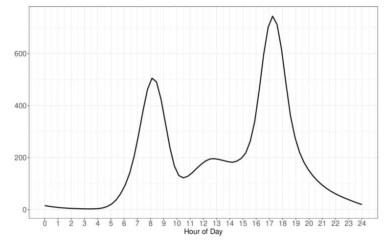
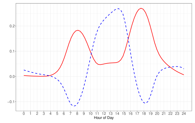
Figure 1: Sample mean function (left plot) and eigenfunctions for the functional principal component analysis (right plot) of the squared distance trajectories at 20 minute intervals of graph Laplacians of daily Divvy bike trip networks in Chicago. In the right plot, the solid red line corresponds to the first eigenfunction, which explains 90.40% of variability in the trajectories and the dashed blue line to the second eigenfunction, which explains 7.28% of the variability.

The predominant directions of variation of the daily Fréchet variance trajectories around the Fréchet mean function are visualized by the first two eigenfunctions in the right plot of Figure 1. The first two functional principal component scores explain about 97.7% of the variation in the Fréchet variance trajectories. The first eigenfunction reflects increased variability around the peaks of the Fréchet variance function that is shown in Figure 1. The peaks are between between 7am to 10am and 4pm to 7pm, which reflect morning and late afternoon and early evening peaks of commute, where the deviations from the mean Fréchet variance function are seen to be largest. The second eigenfunction reflects a contrast between these peaks and the squared deviation from the mean Fréchet variance function during the time period 11am to 4pm.

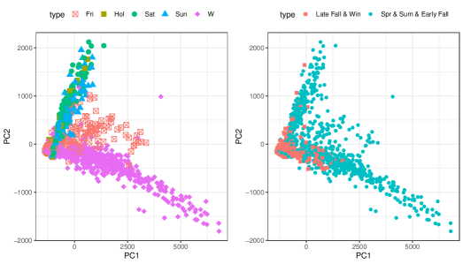
Figure 2: Pairwise plots of the first two FPC scores, distinguished by day of the week (left plot) and by season (right plot). In the left plot, ‘W’ stands for regular Mondays to Thursdays, ‘Fri’ for Fridays, ‘Sat’ for Saturdays, ‘Sun’ for Sundays and ‘Hol’ for special holidays. In the right plot, ‘Late Fall & Win’ includes months between November and March and ‘Spr & Sum & Early Fall’ includes April to October.

Analyzing the FPC scores of the daily Fréchet variance trajectories along the first and second eigenfunctions, Figure 2 reveals several interesting patterns in the daily Fréchet variance trajectories. Weekdays and weekends form distinct clusters. Holidays show patterns similar to weekends. When scrutinizing second versus first FPC scores, an outlying observation is found at August 21, 2017. Researching the background of this day, we found that there was a total solar eclipse, which was in peak view over Chicago at 1:18 pm in the afternoon. The Fréchet variance trajectory of this particular day is illustrated in Figure A.1 in section A.4 of the online supplement. An application of the naive Bayes classifier and the support vector machine on the first two FPC scores of the daily Fréchet variance trajectories with “weekdays” and “weekends and holidays” as the binary response using 75% of the data as training sample and 25% of the data as test sample gave a low misclassification rate of 6.02% in both cases. The classification result is illustrated in Figure A.2 in the online supplement.

We also performed a FPCA of these Fréchet variance trajectories for weekdays, Fridays and weekends, including special holidays in the same group as weekends, separately for the three cases, with results displayed in Figures A.3 and A.4 in the online supplement. Weekdays and weekends, including special holidays, show clear differences in both mean Fréchet variance functions and eigenfunctions. The Friday pattern can be characterized as “transition” from weekdays to weekends. Seasonal differences can impact bike sharing patterns. In the right plot of Figure 2, we display second versus first FPC scores, differentiated according to two broad seasonal groups. Spring, summer and early fall includes months from April to October that exhibit greater variability than the late fall and winter months of November to March, with further illustrations in Figures A.5 and A.6 in the online supplement.

4.2 Fertility Data

The Human Fertility Database provides cohort fertility data for various countries and calendar years. The data are available at www.humanfertility.org and facilitate the study of the time evolution and inter-country differences in fertility over a period spanning more than 30 calendar years (see also Chen et al. 2017). We selected 27 countries with complete fertility records for the time period 1976 to 2009. For each country and year, the age specific total live birth counts correspond to histograms of maternal age with bin size one year. These histograms were smoothed (for which we employed local least squares smoothing using the Hades package available at https://stat.ucdavis.edu/hades/) to obtain smooth probability density functions for maternal age, where we consider the age interval $[12,55]$. We thus obtain samples of time-varying univariate probability distributions, where the subjects are the countries, the time is calendar years between 1976 and 2009 and the observation at each time point for a specific country is its maternal age distribution, i.e., the distribution of ages when females give birth within the age interval $[12,55]$ for the specified country and calendar year.

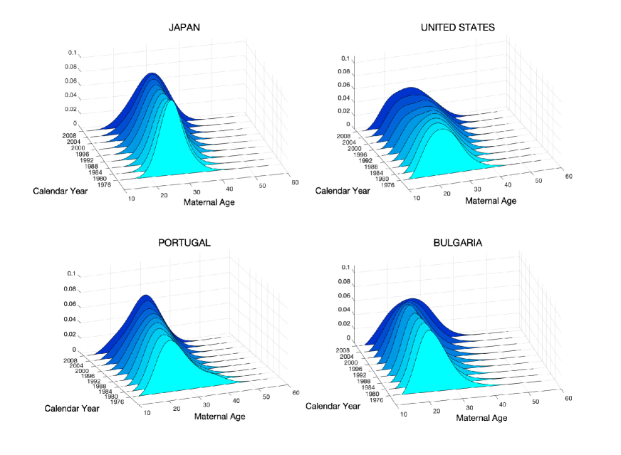
Figure 3: Yearly maternal age distributions represented as density functions for the age interval [12,55] during the time period 1976 to 2009 (selected years). The $x$-axis represents maternal age, the $z$-axis the density functions and the $y$-axis calendar years.

Figure 3 displays the evolving densities for Japan, United States, Portugal and Bulgaria in some selected years over a period spanning 56 years from 1959 to 2014. There are clear differences in the maternal age evolution between countries, but the overall trend is that maternal age increases. This is also reflected in the Fréchet mean densities in Figure 4, which show a shift in their mode locations towards higher age over the years.

We opt for the 2-Wasserstein metric as the distance between probability distributions, which corresponds to the $L^{2}$ distance between their quantile functions, a metric that has proved to be an excellent choice in many applications (Bolstad et al. 2003; Bigot et al. 2018). The sample Fréchet mean trajectory in a particular year then corresponds to the sample average of the quantile functions of the 27 countries in that year (Dubey and Müller 2019a), which is represented as the corresponding density function. We then obtained the Fréchet variance trajectory for each country, where its value for a given calendar year corresponds to the squared 2-Wasserstein distance between the maternal age distribution of the country to the Fréchet mean age distribution for the specified calendar year.

Finally, we performed a FPCA on the 27 country specific Fréchet variance trajectories. Figure 5 shows the estimated mean function of the Fréchet variance trajectories, which is a scalar function that corresponds to the sample average of the Fréchet variance trajectories as a function of calendar year. The predominant directions of variation of the distance trajectories around the Fréchet mean trajectory are captured by the first two eigenfunctions, which are depicted in the left plot of Figure 6. The first and second eigencomponent explain 74.64% and 17.40% of the variation in the distance trajectories. The first eigenfunction is increasing until between 1995 to 2000 and then starts to decrease. This shows increasing deviation of the distance trajectories from the mean Fréchet  variance trajectory until right before the new millennium after which these deviations tend to decrease. The second eigenfunction reflects a contrast between the earlier and later parts of the calendar time interval.

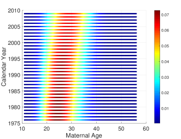
Figure 4: Fréchet mean maternal age distributions represented as a heat plot of density functions for the age interval [12,55] during the time period 1976 to 2009.

The years between 1995 to 2000 mark the critical period when the changes in the mode of maternal age distributions start to take place as displayed in Figure 4. This period of increased activity is also prominent in Figure 5 which shows that the Fréchet variance of maternal age distributions increases in the beginning, reaches a peak between 1995 and 2000 and then starts to decrease. This might be attributed to increasing numbers of women opting for higher education and participating in the labor force in some of the countries included in the dataset over the time interval where the data have been collected. Another likely factor are advanced birth control measures in the past few decades, which led to changes in the maternal age distribution early on for some countries, while these changes were delayed for some other countries, leading to increased discrepancies between countries from 1995 to 2000, which stabilized later as countries moved closer to the mean behavior.

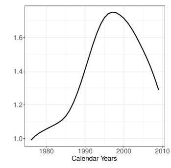
Figure 5: Sample mean function of the Fréchet variance trajectories of the time courses of country specific maternal age distributions.

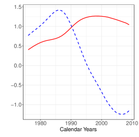
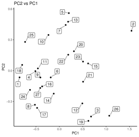
Figure 6: Left panel: First (solid red) and second (blue dashed) eigenfunction of the country specific Fréchet variance trajectories, which explain 74.64% and 17.40% of variability, respectively. Right panel: Second versus first FPC scores of the country specific Fréchet variance trajectories. Here 1 denotes Austria; 2 Bulgaria; 3 Belarus; 4 Canada; 5 Czech Republic; 6 Estoina; 7 Finland; 8 Germany; 9 France; 10 Hungary; 11 Israel; 12 Italy; 13 Japan; 14 Lithuania; 15 Netherlands; 16 Norway; 17 Poland; 18 Portugal; 19 Russia; 20 Slovakia; 21 Spain; 22 Sweden; 23 Switzerland; 24 United Kingdom; 25 Taiwan; 26 Ukraine; 27 United States.

The FPC scores of the trajectories along predominant directions of variation not only reveal interesting patterns but also aid in identifying extremes, which is tricky for the case of time-varying probability distributions. Plotting second versus first FPC scores (right plot of Figure 6), one finds that Bulgaria shows large deviations from the Fréchet mean variance function trajectory along both first and second eigenfunctions. The Czech Republic has the highest second FPC, indicating a large contrast in the distance from the Fréchet mean trajectory between early and later years. Portugal and Austria have negative first FPCs and small second FPCs, which means that their deviation from the Fréchet mean trajectory is less than the average deviation over the calendar time interval.

4.3 Empirical Dynamics

When using FDA for analyzing real valued longitudinal data, a common assumption is that the data are generated by an underlying smooth and square integrable stochastic process. The derivatives of the trajectories of such processes are often the key to understanding the underlying dynamics (Ramsay 2000; Mas and Pumo 2009; Ramsay et al. 2007). Empirical dynamics (Müller and Yao 2010) is a systematic approach to assess the underlying dynamics of longitudinally observed data. It is based on the decomposition

$$Y^{(1)}(t)-\mu^{(1)}(t)=\beta(t)\{Y(t)-\mu(t)\}+Z(t),$$ (9)

where $Y(\cdot)$ is the underlying stochastic process, $\mu(t)=E(Y(t))$, $Y^{(1)}(\cdot)$ and $\mu^{(1)}(\cdot)$ are the derivatives of $Y(\cdot)$ and $\mu(\cdot)$, $\beta(\cdot)$ is a smooth time varying linear coefficient function and $Z(\cdot)$ is a random drift process. For Gaussian processes this decomposition can be easily derived and then $Z$ and $Y$ are independent with $E(Z(t))=0$, leading to

$$E\left[Y^{(1)}(t)-\mu^{(1)}(t)\Big{|}Y(t)\right]=\beta(t)\{Y(t)-\mu(t)\}.$$ (10)

When one has non-Gaussian processes, such as the distance processes $V^{\ast}$ (2), the above decompositions provide useful approximations and can be interpreted in a least squares sense, where the coefficient of determination

$$R^{2}(t)=1-\frac{{\rm var}\{Z(t)\}}{{\rm var}\{Y^{(1)}(t)\}}$$

indicates the fraction of variance explained by the empirical dynamics approximation. On pertinent subdomains where $R^{2}(t)$ is relatively large, the dynamics of the trajectories are determined to a greater extent by the linear model in (10), while otherwise the random drift process $Z$ becomes the driving factor instead of the dynamic equation. The time-varying function $\beta(t)$ summarizes the characteristics of the dynamics of the underlying process. If $\beta(t)<0$, one observes centripetality or dynamic regression to the mean, i.e., a trajectory which is away from the mean function tends to move closer toward the mean function as time progresses. If on the other hand $\beta(t)>0$, one has centrifugality or dynamic explosive behavior, since deviations from the mean at time $t$ tend to increase beyond $t$.

Noting that it is infeasible to define derivatives for trajectories of random objects since the notion of derivative for metric space data is not defined, we apply empirical dynamics instead to the real-valued Fréchet variance trajectories $V^{\ast}$ (2),

$$\frac{d}{dt}(V^{\ast}(t)-EV^{\ast}(t))=\beta(t)(V^{\ast}(t)-EV^{\ast}(t))+Z(t).$$ (11)

We note that centripetality and centrifugality relate to the mean trajectory $EV^{\ast}(t)$, i.e., the mean Fréchet variance function; we quantify the dynamics of the variation relative to this function. For estimation of the time varying coefficient $\beta(\cdot)$ and $R^{2}(t)$, we adopt a plug-in estimation procedure (Liu and Müller 2009; Sentürk and Müller 2010).

We implemented the empirical dynamics model (11) for the sample of time varying maternal age distributions with the R package fdapace. Figure 7 illustrates the estimated slope function $\hat{\beta}(t)$ and coefficient of determination function $\hat{R}^{2}(t)$, where the latter indicates that the dynamics of the maternal age distribution trajectories can be explained by the first order differential equation in the period before 1995 and after 2000, but not in between. The slope function is positive before 2000 and negative after 2000, indicating centrifugality of the maternal age distributions before 2000 and centripetality after 2000, so that in more recent years there is a tendency for the fertility distributions to become more similar in the sense that their variation around the mean distance function is decreasing over calendar time, while the mean distance function itself is also decreasing as seen in Figure 5.

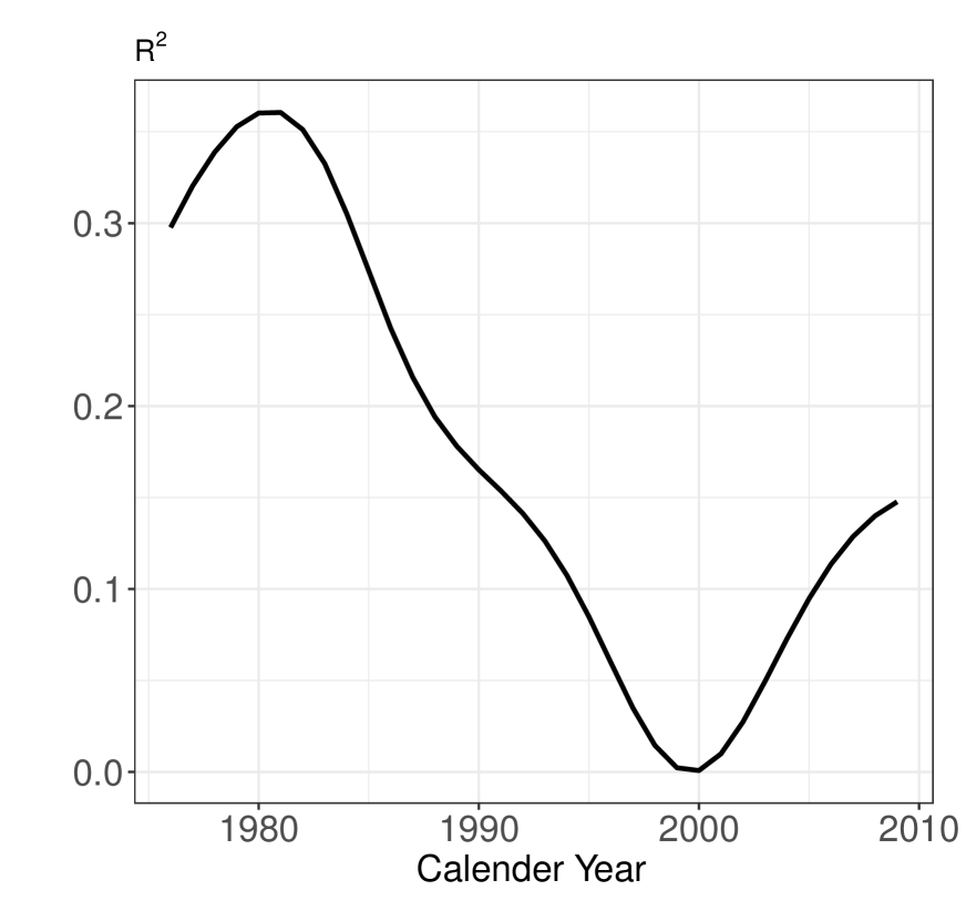
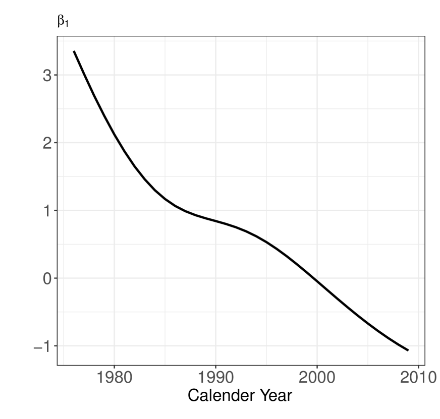
Figure 7: Smooth estimate of the coefficient of determination $R^{2}(t)$ (left) and the varying coefficient function $\beta(t)$(right), capturing empirical dynamics of the distance trajectories of the fertility data.

4.4 Zürich Longitudinal Growth Data

Statistical shape analysis is an emerging field of data analysis that constitutes measuring, describing and comparing random shapes (Dryden and Mardia 2016; Kendall 1984, 1989; Le and Kendall 1993; Patrangenaru and Ellingson 2015; Mardia et al. 2005). Often, shapes are determined using a finite set of coordinate points, known as landmark points. As an example of shapes evolving over time, we consider the growth modalities that are obtained from a longitudinal study on human growth and development (Gasser et al. 1984). This study included growth data for $232$ Swiss children and was conducted in the University Children’s Hospital in Zürich between 1954 and 1978. For each child, we consider trajectories $X_{i}(t)$, where $X_{i}(t)$ is a $4\times 2$ matrix which represents four landmarks in two dimensions. The four landmarks are the foot, which is set to be the point $(0,0)$, the top of the head which has coordinate $(0,\text{standing height})$, the shoulder which is set to have the coordinate $(\text{bi-humeral diameter},0.8\ \text{standing height})$ and the hip which is set at the point $(\text{bi-iliacal diameter},\text{leg length})$. These shape trajectories are observed for the age interval $t\in[0.5,20]$ years.

The trajectories $X_{i}(t)$ described above correspond to two-dimensional landmarks that take values in the planar shape space, which can be viewed as configurations on the complex plane. In this space, we adopt the full Procrustes metric, which has been quite successful in the analysis of planar shapes in a wide variety of applications (Dryden and Mardia 2016). Given centered complex configurations $y=(y_{1},y_{2},\dots,y_{k})$ and $z=(z_{1},z_{2},\dots,z_{k})$, both in $\mathbb{C}^{k}$, with $y^{*}1_{k}=0=z^{*}1_{k}$, the full Procrustes distance between $y$ and $z$ is defined as

$$d_{\mathcal{P}}(y,z)=\left\{1-\frac{y^{*}zz^{*}y}{z^{*}zy^{*}y}\right\}^{1/2}.$$

Accordingly, we first obtained the sample Fréchet mean trajectory of the random shape trajectories under the full Procrustes metric as

$$\hat{\mu}(t)=\operatorname*{argmin}_{\omega\in\Omega}\frac{1}{n}\sum_{i=1}^{n}d^{2}_{\mathcal{P}}(X_{i}(t),\omega),$$

and then analyzed the subject specific Fréchet variance trajectories $d^{2}(X_{i}(t),\hat{\mu}(t)),t\in[0.5,20],i=1,2,\dots,232$ using the tools developed in this paper. The sample Fréchet mean and the computation of the full Procrustes distance were carried out using the R package shapes (Dryden 2012). For details on existence and uniqueness of Fréchet means in shape spaces see Le (1995, 1998).

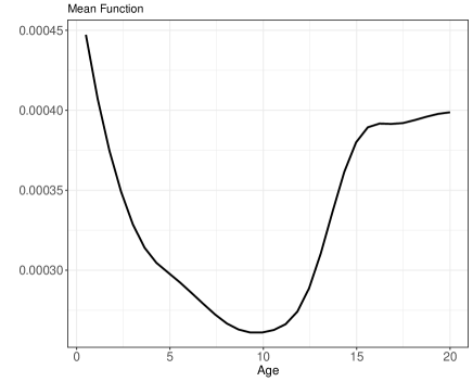
Figure 8: Sample mean function of the Fréchet variance trajectories of the time courses of shape data representing growth modalities.

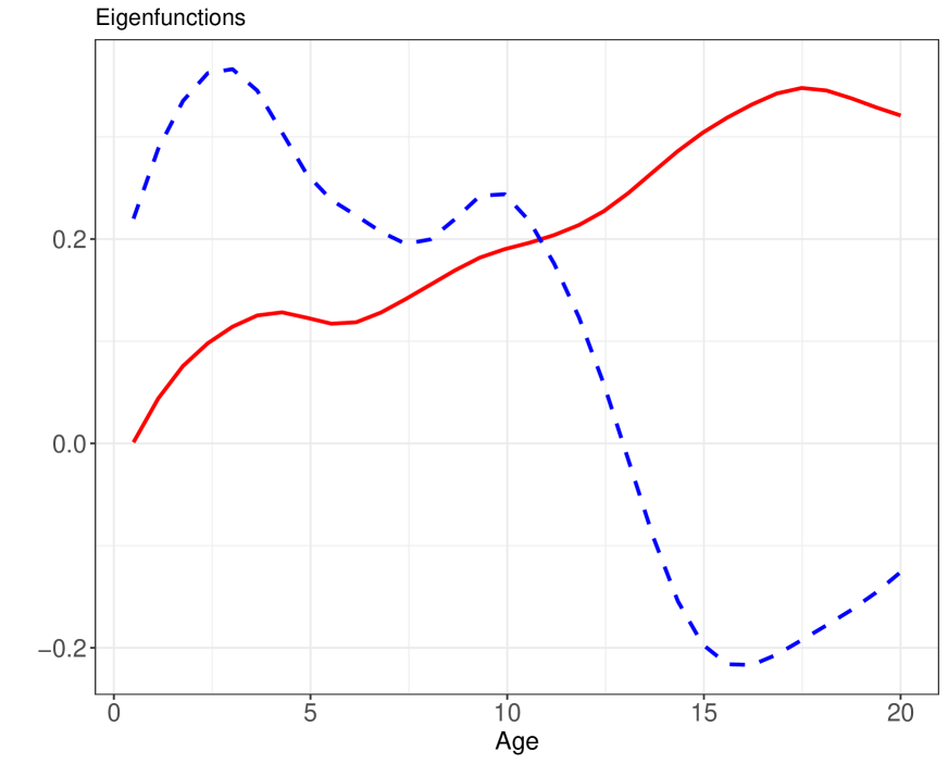
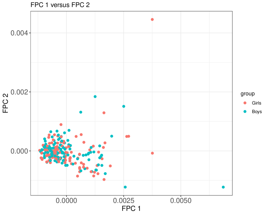
Figure 9: Left panel: First (solid red) and second (blue dashed) eigenfunction of the child specific Fréchet variance trajectories, which explain 76.07% and 18.55% of variability, respectively. Right panel: Second versus first FPC scores of the child specific Fréchet variance trajectories.

Figure A.1 shows the time evolution of population Fréchet variance, which captures the overall variability trends of the shape trajectories around the Fréchet mean trajectory. The periods of early childhood, that is from infancy to about 5 years of age, and the period starting at adolescence until adulthood, i.e. between 13 to 20 years, exhibit greater variability around the Fréchet mean shapes. Figure A.2 show the first two dominant eigenfunctions, which explain 76.07% and 18.55% of the variability in the subject specific Fréchet variance trajectories. The corresponding plot of the second FPC score versus the first FPC score shows that there is no systematic difference between boys and girls when comparing the shape trajectories under the full Procrustes metric.

To illustrate the growth shape patterns, we select four boys as indicated in the left panel of Figure A.3 with the first FPC scores ranging from positive to zero to negative. A negative first FPC score of the subject specific Fréchet variance trajectories loads negatively on the first eigenfunction illustrated in Figure A.2, which highlights growth patterns that are closer to the sample Fréchet mean shape trajectory than average. A first FPC score closer to zero is associated with subjects that exhibit close to average variability around the sample Fréchet mean shape over time, while a positive first FPC score suggests greater than average variability around the mean Fréchet mean trajectory. The four boys “1”,“2”, “3” and “4” illustrated in Figure A.3 fit these prototypes. While “1” is closest to the sample Fréchet mean shape trajectory, “2” represents a child who shows typical deviation around the Fréchet mean shape over the years, whereas “3” exhibits larger than typical variation over the years and “4” stands out from the rest with an extremely high first FPC score. This pattern suggests that the first FPC captures differences in overall size of the children.

Figure A.4 illustrates variability with respect to the second eigenfunction, which corresponds to a contrast between early and later years (Figure A.2). for three selected boys highlighted in the left panel, all of whom have small first FPC scores, and whose second FPC scores vary from negative to zero to positive. For these boys, ‘5” tends to remain thinner during the teenage years as compared to“6” whose hip diameter gets wider during the teenage years, while “7” has the biggest growth in hip diameter among the three.

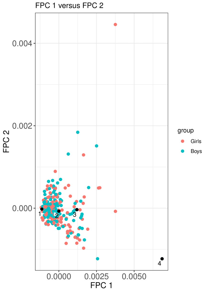
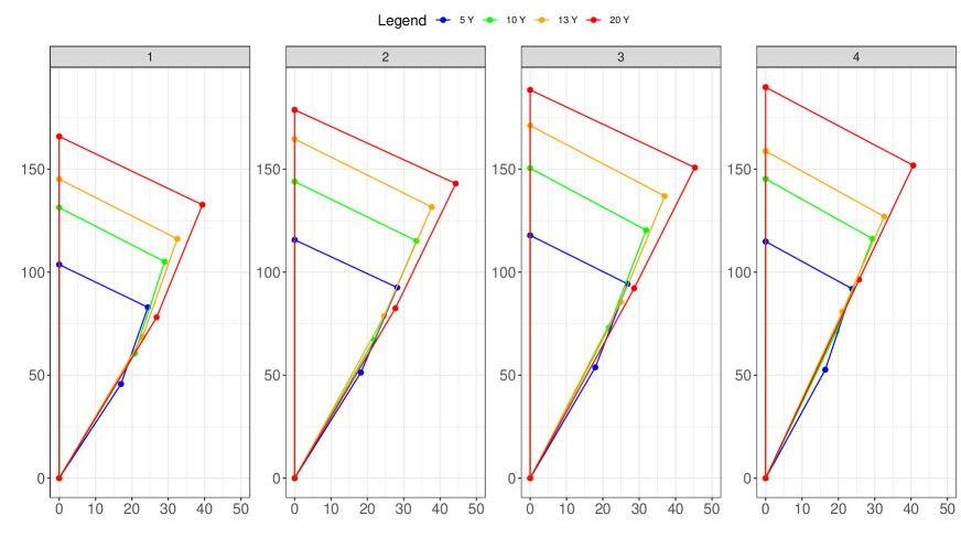
Figure 10: Left panel: Four selected children (black dots). Right panel: The shape trajectories $X_{i}(t),t=5,10,13,20$ for the four selected children in the left panel.

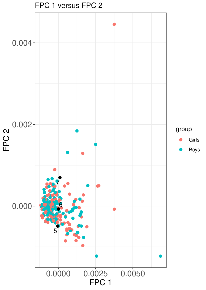
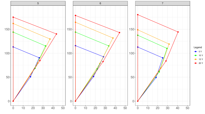
Figure 11: Left panel: Three selected children (black dots). Right panel: The shape trajectories $X_{i}(t),t=5,10,13,20$ for the three selected children in the left panel.

We also implemented empirical dynamics for these shape data. Figure A.6 illustrates the slope function $\hat{\beta}(t)$ and the coefficient of determination $\hat{R}^{2}(t)$. The latter shows that dynamics in the distance trajectories between the mean shape trajectory and the subject specific shape trajectories can be explained to a large extent by a first order differential equation for the age range 5 to 15 years. The slope function $\hat{\beta}(t)$ is positive until 17 years of age and negative thereafter, indicating centrifugality of the distance trajectories between infancy and late teenage years, where children’s shapes diverge, and centripetality near adulthood.

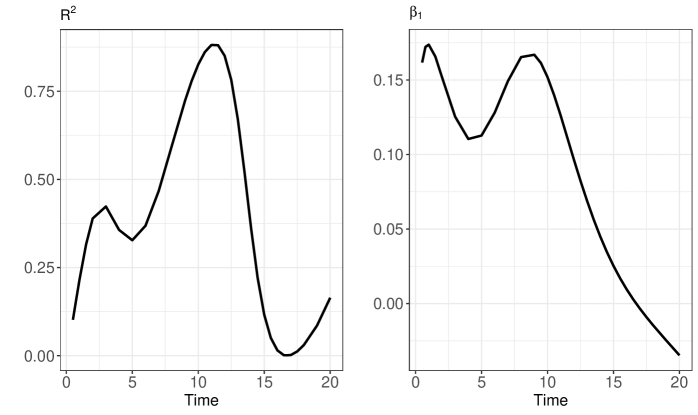
Figure 12: Smooth estimate of the coefficient of determination $R^{2}(t)$ (left) and the varying coefficient function $\beta(t)$(right), capturing empirical dynamics of the distance trajectories of the longitudinal growth shape data.

5. SIMULATIONS

We illustrate our methods by simulations using samples of time-varying networks with 20 nodes, inspired by many real world networks that exhibit community structure, where communities are groups of nodes in a network that show increased within group connectivity and decreased between group connectivity. Existence of community structure is for example prevalent in traffic networks, particularly the bike networks that we study in our data applications, and also brain networks, social networks and many other areas where networks arise. We generated the time varying networks as follows.

Step 1. Three groups of time-varying networks with 20 nodes differing in the community membership of the nodes were generated. Indexing the nodes of the networks by $1,2,\dots,20$ and the communities by $C_{1},C_{2},C_{3},C_{4}$ and $C_{5}$, the community membership composition of the nodes for the three groups of networks was as follows,

Group 1: Five communities, $C_{1}=\{1,2,3,4\}$, $C_{2}=\{5,6,7,8\}$, $C_{3}=\{9,10,11,12\}$, $C_{4}=\{13,14,15,16\}$ and $C_{5}=\{17,18,19,20\}$.

Group 2: Four communities, $C_{1}=\{1,2,3,4,5,6,7,8\}$, $C_{2}=\{9,10,11,12\}$, $C_{3}=\{13,14,15,16\}$ and $C_{4}=\{17,18,19,20\}$.

Group 3: Three communities, $C_{1}=\{1,2,3,4\}$, $C_{2}=\{5,6,7,8\}$ and
$C_{5}=\{9,10,11,12,13,14,15,16,17,18,19,20\}$.

We let the community memberships of the nodes stay fixed in time, while the edge connectivity strengths $W_{jj^{\prime}}(t)$ between the communities change with time. The time-varying connectivity weights $W_{jj^{\prime}}(t)$ between communities $C_{j}$ and $C_{j}^{\prime}$, $j,j^{\prime}\in\{1,2,3,4,5\}$, that we used when generating the random networks are illustrated in Figure 13. The intra-community connection strengths are higher than the inter-community strengths over the entire time interval. Such dynamic connectivity patterns are encountered in brain networks (Calhoun et al. 2014), where densely connected brain regions form communities or hubs and inter-hub connectivity often exhibit changing patterns with age.

Step 2. The network adjacency matrices $A_{i}(t)$ are generated as:

$$(A_{i}(t))_{k,l}=W_{j,j^{{}^{\prime}}}(t)\left\{\frac{1+\text{sin}(\pi(t+U_{i,kl})V_{i,kl})}{D}\right\},\ t\in[0,1],$$

where $C_{j}$ is the community membership of node $k$ and $C_{j}^{{}^{\prime}}$ is the community membership of node $l$, $W_{j,j^{{}^{\prime}}}(t)$ is the edge connectivity strength between nodes in communities $C_{j}$ and $C_{j}^{\prime}$, $U_{i,kl}$ follows $U(0,1)$ and $V_{i,kl}$ is $1$ if $j=j^{\prime}$ and sampled uniformly from $\{5,6,\dots,15\}$ if $j\neq j^{\prime}$. If $j=j^{\prime}$, we set $D=2$, otherwise $D=4$. Here $U_{i,kl}$ and $V_{i,kl}$ determine random phase and frequency shifts of the sine function which regulate at what times and how often the edge weights are zero. As $V_{i,kl}$ increases, so does the frequency of the times within $[0,1]$ at which the edge weight is zero. The trajectories are represented as graph Laplacians

$$X_{i}(t)=D_{i}(t)-A_{i}(t),$$

where $D_{i}(t)$ is a diagonal matrix whose diagonal elements are equal to the sum of the corresponding row elements in $A_{i}(t)$. Adopting the Frobenius metric in the space of graph Laplacians, the Fréchet mean network at time $t$ is the pointwise average of the graph Laplacians at time $t$, and we obtain the Frobenius distance trajectories of the individual subjects from the Fréchet mean trajectory.

Step 3. We carry out FPCA of the distance trajectories generated in Step 2.

The results are shown in Figure 14. The proposed method is seen to perform well in recovering the groups in the scatter plot of the second versus first functional principal component. Groups 1 and 2 are found to have closer cluster centers than groups 1 and 3. This is explained by the fact that group 2 is obtained from group 1 by merging $C_{1}$ and $C_{2}$ in group 1, which show more similarities than when merging $C_{3}$, $C_{4}$ and $C_{5}$ in group 1 to form group 3.

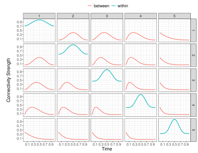
Figure 13: Time varying connectivity weights between the five communities $C_{1},C_{2},\dots,C_{5}$.

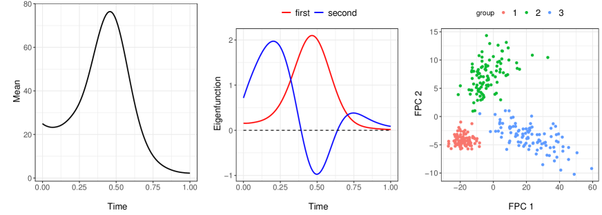
Figure 14: Mean function (left), eigenfunctions (middle) and the scatter plot of second versus first FPC (right) obtained from functional principal component analysis of the distance trajectories for networks. The red line corresponds to the first eigenfunction and the blue line to the second.

6. DISCUSSION

We provide a framework for the analysis of time-varying object data, where the random objects can take values in a general metric space, by defining a generalized notion of mean function in the object space. The key to our approach is that functional data analysis methodology can be applied to squared distance functions of the subject specific curves from the mean function, elucidating the nature of the object time courses, including empirical dynamics, identifying clusters, and detecting extremes and potential outliers in a sample of object trajectories. Another important application is to determine time-specific ranks for subjects, in terms of the distance of the subject’s trajectory from the mean trajectory; such ranks have important applications in health monitoring, for example in neurodevelopment (Dosman et al. 2012). The FPCs that we obtain for time-varying random objects can also be used for regression analysis, where object time courses are responses or possibly predictors.

As pointed out by a referee, another possible interpretation of empirical dynamics can be gained with the notion of antimeans. For compact metric spaces, when the extreme values of the Fréchet function $E(d^{2}(Y,\omega))$ are attained in $\Omega$, the set of maximizers of the Fréchet function forms a newly introduced notion of location parameter called the Fréchet antimean set (Wang et al. 2020; Patrangenaru et al. 2016a, b). Just like Fréchet means, Fréchet antimeans can form useful statistics for describing and comparing samples of object data, as has been illustrated for samples of shapes of lily flowers (Patrangenaru et al. 2016b). For data that reside in compact manifolds where the notion of the data center is obscure, Fréchet antimeans could provide constructive data summaries. Hence once could frame empirical dynamics with respect to not only the Fréchet means, but also the Fréchet antimeans, which might uncover insightful findings in terms of regression to the mean or the antimean, leading to multiple points of interest. In such situations, in the context of centrifugality, one might tend to move closer to the Fréchet antimean, for which anticentripetality might be a fitting term.

Our data examples include samples of time-varying univariate probability distributions and samples of time evolving networks. In practice the object functions may not be fully observed, but instead are observed on a more or less dense time grid, possibly with noise. In such situations one can opt for smoothing the object trajectories if the observation grid is sufficiently dense. To implement preliminary smoothing and interpolation, Fréchet regression provides a possible option (Petersen and Müller 2019). While the role of smoothing individual trajectories in FDA is well understood in the Euclidean case (Hall and Van Keilegom 2007; Zhang and Chen 2007), it remains an open problem to investigate its properties in the much more general setting of longitudinal object data. An even bigger challenge that is also left for future research is the case where measurement grids are sparse and irregular, a problem that was recently studied in Lin et al. (2020); Dai et al. (2020) for data on Riemannian manifolds.

ONLINE SUPPLEMENT

A.1 Overview of the Theoretical Derivations

For an element $\omega$ taking values in $\Omega$ and $s\in[0,1]$, define

$$U_{n}(\omega,s)=\frac{1}{n}\sum_{i=1}^{n}f_{\omega,s}(X_{i})\ \text{and}\ U(\omega,s)=E\{f_{\omega,s}(X)\}$$ (12)

where $f_{\omega,s}(x)=d^{2}(x(s),\omega)-d^{2}(x(s),\mu(s))$. In our setting, $\hat{\mu}(s)$ is the minimizer of $U_{n}(\omega,s)$ and $\mu(s)$ is the minimizer of $U(\omega,s)$. A critical step in establishing uniform convergence of the plug-in estimator of the Fréchet covariance surface $\tilde{C}$ in (6) given by $\hat{C}$ (7) is to find an upper bound for the quantity $E\left(\operatornamewithlimits{sup}_{s\in[0,1],\,\omega\in\Omega:\,d(\omega,\mu(s))<\delta}\left|U_{n}(\omega,s)-U(\omega,s)\right|\right)$ for $\delta>0$. For this, it is convenient to consider function classes

$$\mathcal{F}_{\delta}=\{f_{\omega,s}:s\in[0,1],\,d(\omega,\mu(s))<\delta\}$$ (13)

and to apply empirical process theory. An envelope function for this class is the constant function $F(x)=2M\delta$, where $M$ is the diameter of $\Omega$. The $L_{2}$ norm of the envelope function is $||F||_{2}=2M\delta$.

By Theorem 2.14.2 of Van der Vaart and Wellner (1996),

$$E\left(\operatornamewithlimits{sup}_{s\in[0,1],\,\omega\in\Omega:\,d(\omega,\mu(s))<\delta}\left|U_{n}(\omega,s)-U(\omega,s)\right|\right)\leq\frac{2M\delta\ J_{[]}(1,\mathcal{F}_{\delta},L_{2}(P))}{\sqrt{n}},$$ (14)

where $J_{[]}(1,\mathcal{F}_{\delta},L_{2}(P))$ is the bracketing integral of the function class $\mathcal{F}_{\delta}$, which is

$$J_{[]}(1,\mathcal{F}_{\delta},L_{2}(P))=\int_{0}^{1}\sqrt{1+\log N(\varepsilon||F||_{2},\mathcal{F}_{\delta},L_{2}(P))}d\varepsilon.$$

Here $N(\varepsilon||F||_{2},\mathcal{F}_{\delta},L_{2}(P))$ is the minimum number of balls of radius $\varepsilon||F||_{2}$ required to cover the function class $\mathcal{F}_{\delta}$ under the $L_{2}(P)$ norm. Assumptions (A2)-(A4) imply

$$J_{[]}(1,\mathcal{F}_{\delta},L_{2}(P))=O(\sqrt{\log{1/\delta}})\quad\text{as}\quad\delta\rightarrow 0;$$ (15)

see Lemma 4 in Section A.3.

Equation (15) provides a key result for obtaining the rate of convergence of $\hat{\mu}$. One can show that under assumptions (A1)-(A4),

$$\sup_{s\in[0,1]}d(\hat{\mu}(s),\mu(s))=O_{P}\left(\left(\frac{\sqrt{\log{n}}}{n}\right)^{\frac{1}{2(\beta-1)}}\right),$$ (16)

with $\beta$ as in (A2); see Lemma 5 in Section A.3.

In Lemma 1 in Section A.2 we establish the uniform convergence of the process $\frac{1}{n}\sum_{i=1}^{n}d^{2}(X_{i}(s),\hat{\mu}(s))$ to $\frac{1}{n}\sum_{i=1}^{n}d^{2}(X_{i}(s),\mu(s))$. This is the main step to derive the uniform convergence of the sample based Fréchet covariance surface $\hat{C}(s,t)$ in (7) to the oracle Fréchet covariance surface $\tilde{C}(s,t)$ in (6) (see Lemma 2).

A.2 Proofs of Theorem 1 and 2

Proof of Theorem 1.

For Theorem 1, we need two additional Lemmas:

Lemma 1 (Convergence of sample Fréchet variance function).

Under assumptions (A1)-(A4),

$$\sup_{s\in[0,1]}\sqrt{n}\left|\frac{1}{n}\sum_{i=1}^{n}\{V_{i}(s)-V_{i}^{*}(s)\}\right|=o_{P}(1).$$

Proof of Lemma 1.

Let $\varepsilon>0$ and $\delta>0$. Observe

$$P\left(\sup_{s\in[0,1]}\sqrt{n}\left|\frac{1}{n}\sum_{i=1}^{n}d^{2}(X_{i}(s),\hat{\mu}(s))-\frac{1}{n}\sum_{i=1}^{n}d^{2}(X_{i}(s),\mu(s))\right|>\varepsilon\right)$$

$$=P\left(\inf_{s\in[0,1]}\left(\frac{1}{n}\sum_{i=1}^{n}d^{2}(X_{i}(s),\hat{\mu}(s))-\frac{1}{n}\sum_{i=1}^{n}d^{2}(X_{i}(s),\mu(s))\right)<-\frac{\varepsilon}{\sqrt{n}}\right)$$

$$\leq P\left(\inf_{s\in[0,1],\,\omega\in\Omega:\,d(\omega,\mu(s))<\delta}\left(\frac{1}{n}\sum_{i=1}^{n}d^{2}(X_{i}(s),\omega)-\frac{1}{n}\sum_{i=1}^{n}d^{2}(X_{i}(s),\mu(s))\right)<-\frac{\varepsilon}{\sqrt{n}}\right)$$

$$+P\left(\sup_{s\in[0,1]}d(\hat{\mu}(s),\mu(s))>\delta\right)$$

$$\leq P\left(\sup_{s\in[0,1],\,\omega\in\Omega:\,d(\omega,\mu(s))<\delta}\left|U_{n}(\omega,s)-U(\omega,s)\right|>\frac{\varepsilon}{\sqrt{n}}\right)+P\left(\sup_{s\in[0,1]}d(\hat{\mu}(s),\mu(s))>\delta\right).$$ (17)

This is because $\inf_{s\in[0,1],\,\omega\in\Omega:\,d(\omega,\mu(s))<\delta}\{E(d^{2}(X(s),\omega))-E(d^{2}(X(s),\mu(s))\}=0$ implies

$$\sup_{s\in[0,1],\,\omega\in\Omega:\,d(\omega,\mu(s))<\delta}\left|U_{n}(\omega,s)-U(\omega,s)\right|$$

$$\geq\left|\inf_{s\in[0,1],\,\omega\in\Omega:\,d(\omega,\mu(s))<\delta}U_{n}(\omega,s)-\inf_{s\in[0,1],\,\omega\in\Omega:\,d(\omega,\mu(s))<\delta}U(\omega,s)\right|.$$

Continuing from equation (17), we find that the second term goes to zero due to Lemma 3 in Section A.3. Using Markov inequality, equation (14) and Lemma 4 in Section A.3 , by choosing $\delta$ sufficiently small, the first term is upper bounded by

$$\frac{\sqrt{n}E\left(\sup_{s\in[0,1],\,\omega\in\Omega:\,d(\omega,\mu(s))<\delta}\left|U_{n}(\omega,s)-U(\omega,s)\right|\right)}{\epsilon}\leq\frac{2M\delta J_{[]}(1,\mathcal{F}_{\delta},L_{2}(P))}{\epsilon}.$$ (18)

Given any $\varepsilon>0,h>0$, we aim to show that there exists a sufficiently large integer $N$ such that for all $n\geq N$ we have

$$P\left(\sup_{s\in[0,1]}\sqrt{n}\left|\frac{1}{n}\sum_{i=1}^{n}d^{2}(X_{i}(s),\hat{\mu}(s))-\frac{1}{n}\sum_{i=1}^{n}d^{2}(X_{i}(s),\mu(s))\right|>\varepsilon\right)<h.$$

To do this we first choose $\delta$ small enough such that $\frac{2M\delta J_{[]}(1,\mathcal{F}_{\delta},L_{2}(P))}{\epsilon}<\frac{h}{2}$ and then choose $N$ large enough such that $P\left(\sup_{s\in[0,1]}d(\hat{\mu}(s),\mu(s))>\delta\right)<\frac{h}{2}$. This completes the proof. ∎

Lemma 2 (Convergence of sample Fréchet covariance surface).

Under assumptions (A1)-(A4),

$$\sqrt{n}\sup_{s,t\in[0,1]}\left|\hat{C}(s,t)-\tilde{C}(s,t)\right|=o_{P}(1).$$

Proof of Lemma 2.

Observe that

$$\sqrt{n}\sup_{s,t\in[0,1]}\left|\hat{C}(s,t)-\tilde{C}(s,t)\right|\leq\sqrt{n}\sup_{s,t\in[0,1]}A_{1}(s,t)+2M^{2}\sqrt{n}\sup_{s\in[0,1]}A_{2}(s),$$

where $A_{1}(s,t)$ and $A_{2}(s)$ are given by

$$A_{1}(s,t)=\left|\frac{1}{n}\sum_{i=1}^{n}d^{2}(X_{i}(s),\hat{\mu}(s))d^{2}(X_{i}(t),\hat{\mu}(t))-\frac{1}{n}\sum_{i=1}^{n}d^{2}(X_{i}(s),{\mu}(s))d^{2}(X_{i}(t),{\mu}(t))\right|,$$

$$A_{2}(s)=\left|\frac{1}{n}\sum_{i=1}^{n}d^{2}(X_{i}(s),\hat{\mu}(s))-\frac{1}{n}\sum_{i=1}^{n}d^{2}(X_{i}(s),{\mu}(s))\right|.$$

By Lemma 1, it is enough to show $\sqrt{n}\sup_{s,t\in[0,1]}A_{1}(s,t)$ converges in probability to zero. As

$$\sqrt{n}\sup_{s,t\in[0,1]}A_{1}(s,t)\leq M^{2}\sqrt{n}\sup_{s\in[0,1]}A_{2}(s)+M^{2}\sqrt{n}\sup_{t\in[0,1]}A_{2}(t)$$

the proof is complete by Lemma 1. ∎

We prove the result in Theorem 1 in three steps.

Step 1: Covariance Operators. We first observe that ${C}(s,t)$ is the covariance function of a second order stochastic process $\{Y(s)\}_{s\in[0,1]}$ where $Y(s)=d^{2}(X(s),\mu(s))$ for $s\in[0,1]$ and has mean function $E(Y(s))=E(d^{2}(X(s),\mu(s)))$. The process $\{Y(s)\}_{s\in[0,1]}$ can also be viewed as a random element $\mathcal{Y}\in\mathcal{L}^{2}[0,1]$ with mean $m=E\mathcal{Y}$ and covariance operator generated by the covariance function $C(s,t)$ denoted by $\mathcal{C}$. Let $\mathcal{Y}_{1},\mathcal{Y}_{2},\dots,\mathcal{Y}_{n}$ be i.i.d. realizations of $\mathcal{Y}$ from which one obtains the sample covariance operator $\tilde{\mathcal{C}}$, the covariance operator generated by $\tilde{C}(s,t)$. By the boundedness of the metric, we have $E(||\mathcal{Y}||^{4})<\infty$ and therefore by Theorem 8.1.2 of Hsing and Eubank (2015), $\sqrt{n}(\tilde{\mathcal{C}}-\mathcal{C})$ converges weakly to a Gaussian random element with mean zero and covariance operator given by

$$\mathcal{R}=E\left(((\mathcal{Y}-m)\otimes(\mathcal{Y}-m)-\mathcal{C})\otimes_{HS}((\mathcal{Y}-m)\otimes(\mathcal{Y}-m)-\mathcal{C})\right).$$ (19)

This is equivalent to saying that $\sqrt{n}\left(\tilde{C}(s,t)-C(s,t)\right)$ has a Gaussian process limit with mean zero and covariance operator

$$\mathcal{R}_{(s_{1},t_{1}),(s_{2},t_{2})}=\mathrm{Cov}\left((Y(s_{1})-m(s_{1}))(Y(t_{1})-m(t_{1})),(Y(s_{2})-m(s_{2}))(Y(t_{2})-m(t_{2}))\right),$$

where $Y(s)=d^{2}(X(s),\mu(s))$ and $m(s)=E(Y(s))$.

Step 2: Convergence of the Marginals to a Multivariate Normal Distribution. For any integer $k$ and any $(s_{1},t_{1}),(s_{2},t_{2}),\ldots,(s_{k},t_{k})\in[0,1]^{2}$, let $C_{i}=C(s_{i},t_{i}),$ $\hat{C}_{i}=\hat{C}(s_{i},t_{i})$ and $\tilde{C}_{i}=\tilde{C}(s_{i},t_{i})$, and further $C^{k}=\left(C_{1},C_{2},\ldots,C_{k}\right)$, $\hat{C}^{k}=\left(\hat{C}_{1},\hat{C}_{2},\ldots,\hat{C}_{k}\right)$ and $\tilde{C}^{k}=\left(\tilde{C}_{1},\tilde{C}_{2},\ldots,\tilde{C}_{k}\right)$. Observe that

$$\sqrt{n}\left(\hat{C}^{k}-C^{k}\right)=\sqrt{n}\left(\hat{C}^{k}-\tilde{C}^{k}\right)+\sqrt{n}\left(\tilde{C}^{k}-C^{k}\right),$$

where the first term converges to zero in probability as a consequence of Lemma 2 and the second term converges in distribution to a multivariate normal distribution with mean zero and covariance matrix $\Sigma^{k}=(\Sigma^{k}_{ij})$, where $\Sigma^{k}_{ij}=\mathcal{R}_{(s_{i},t_{i}),(s_{j},t_{j})}$ as a consequence of Step 1. Therefore by Slutsky’s theorem for any integer $k$ and any $(s_{1},t_{1}),(s_{2},t_{2}),\ldots,(s_{k},t_{k})\in[0,1]^{2}$, $\sqrt{n}\left(\hat{C}^{k}-C^{k}\right)$ converges in distribution to $N(0,\Sigma^{k})$.

Step 3: Uniform Asymptotic Equicontinuity of the Process $\sqrt{n}\left(\hat{C}(s,t)-C(s,t)\right)$.
Let $(s_{1},t_{1}),(s_{2},t_{2})\in[0,1]^{2}$ be such that $|s_{1}-s_{2}|+|t_{1}-t_{2}|<\delta$ for some $\delta>0$. We need to show that for any $S>0$ and as $\delta\rightarrow 0$,

$$\limsup_{n\rightarrow\infty}P\left(\sup_{|s_{1}-s_{2}|+|t_{1}-t_{2}|<\delta}\sqrt{n}\left|\hat{C}(s_{1},t_{1})-C(s_{1},t_{1})-\hat{C}(s_{2},t_{2})+C(s_{2},t_{2})\right|>2S\right)\rightarrow 0.$$ (20)

This is true because

$$\limsup_{n\rightarrow\infty}P\left(\sup_{|s_{1}-s_{2}|+|t_{1}-t_{2}|<\delta}\sqrt{n}\left|\hat{C}(s_{1},t_{1})-C(s_{1},t_{1})-\hat{C}(s_{2},t_{2})+C(s_{2},t_{2})\right|>2S\right)$$

$$\leq A_{\delta}+B_{\delta},$$

where $A_{\delta}=\limsup_{n\rightarrow\infty}P\left(2\sup_{(s,t)\in[0,1]}\sqrt{n}\left|\hat{C}(s,t)-\tilde{C}(s,t)\right|>S\right)$ and $B_{\delta}=$
$\limsup_{n\rightarrow\infty}P\left(\sup_{|s_{1}-s_{2}|+|t_{1}-t_{2}|<\delta}\sqrt{n}\left|\tilde{C}(s_{1},t_{1})-C(s_{1},t_{1})-\tilde{C}(s_{2},t_{2})+C(s_{2},t_{2})\right|>S\right)$.
By Lemma 2, we have $A_{\delta}=0$ for any $S>0$ and from Step 1, the uniform asymptotic equicontinuity of the process $\sqrt{n}\left(\tilde{C}(s,t)-C(s,t)\right)$ implies $B_{\delta}\rightarrow 0$ as $\delta\rightarrow 0$ for any $S>0$.

From Steps 1-3 and Theorems 1.5.4 and 1.5.7 in Van der Vaart and Wellner (1996) the result follows. ∎

Proof of Theorem 2.

For any $j$, perturbation theory as stated for example in Lemma 4.3 of Bosq (2000) gives $|\hat{\lambda}_{j}-\lambda_{j}|\leq\sup_{s,t\in[0,1]}\left|\hat{C}(s,t)-C(s,t)\right|$. Along with Theorem 1 this implies $|\hat{\lambda}_{j}-\lambda_{j}|=O_{P}(1/\sqrt{n}).$ For any $j$, one also has

$$\sup_{s\in[0,1]}\left|\hat{\phi}_{j}(s)-\phi_{j}(s)\right|\leq 2\sqrt{2}\delta_{j}^{-1}\sup_{s,t\in[0,1]}\left|\hat{C}(s,t)-C(s,t)\right|.$$

Applying Theorem 1 and assumption (A5) leads to

$$\sup_{s\in[0,1]}\left|\hat{\phi}_{j}(s)-\phi_{j}(s)\right|=O_{P}(1/\delta_{j}\sqrt{n}).$$ (21)

Next we show the convergence of the scores $\hat{B}_{ij}$ to their population targets $B_{ij}$. For this consider the functions $g_{s}(x)=d^{2}(x(s),\mu(s))$ and the function class $\mathcal{F}=\{g_{s}:s\in[0,1]\}$. Then

$$|f_{s}(x)-f_{t}(x)|\leq 2M(d(x(s),x(t))+d(\mu(s),\mu(t))).$$

Following the arguments in the proof of Lemma 5 in Section A.3, under assumptions (A2) and (A3), whenever $|s-t|<\left(\frac{\rho}{K}\right)^{\beta/\alpha}$, we have with $K=\left\{4MD^{-1}E(G(X))\right\}^{1/\beta}$

$$d(\mu(s),\mu(t))\leq K|s-t|^{\frac{\alpha}{\beta}},$$

where $\alpha$, $\beta$, $\rho$, $D$ and $G(\cdot)$ are as defined in assumptions (A2) and (A3). For $0<u<1$, if $s_{1},s_{2},\ldots,s_{K}$ is a $\left(\frac{\rho u}{K}\right)^{\frac{\beta}{\alpha}}$-net for $[0,1]$ with metric $|\cdot|$ , then for any $s\in[0,1]$ one can find $s_{j}\in[0,1]$ such that

$$|f_{s}(x)-f_{s_{j}}(x)|\leq 2M\left\{G(x)\left(\frac{\rho u}{K}\right)^{\beta}+K\left(\frac{\rho u}{K}\right)\right\}\leq G^{\prime}(x)u,$$

where $G^{\prime}(x)=2M\left\{G(x)\left(\frac{\rho}{K}\right)^{\beta}+K\left(\frac{\rho}{K}\right)\right\}$. Hence the brackets $[f_{s_{i}}\pm G^{\prime}u]$ cover the function class $\mathcal{F}$ and are of size $2||G^{\prime}||_{L_{2}}u$, implying that for some constant $C^{\prime}$,

$$N_{[]}(u,\mathcal{F},L_{2}(P))\leq N\left(\left(\frac{\rho u}{2||G^{\prime}||_{L_{2}}K}\right)^{\frac{\beta}{\alpha}},[0,1],|\cdot|\right)\leq\frac{C^{\prime}}{u^{\frac{\beta}{\alpha}}}.$$

Here $N_{[]}(\varepsilon,\mathcal{F},L_{2}(P))$ is the bracketing number, defined in Van der Vaart and Wellner (1996) as the minimum number of $\varepsilon$-brackets needed to cover $\mathcal{F}$, where an $\varepsilon$-bracket is composed of pairs of functions $[l,u]$ such that $||l-u||_{L_{2}}<\varepsilon$. Then

$$\int_{0}^{1}\sqrt{\log N_{[]}(u,\mathcal{F},L_{2}(P))}du$$

$$\leq \int_{0}^{1}\sqrt{\log C^{\prime}-\frac{\beta}{\alpha}\log u}\ du\leq\sqrt{\log C^{\prime}}+\int_{0}^{1}\sqrt{-\frac{\beta}{\alpha}\log u}\ du$$

$$= \sqrt{\log C^{\prime}}+\sqrt{\frac{\beta}{\alpha}}\int_{0}^{\infty}x^{1/2}e^{-x}dx\,\,<\,\,\infty.$$

By Theorem 3.1 in Ossiander (1987) we have that $\mathcal{F}$ has the Donsker property and therefore $\frac{1}{\sqrt{n}}\sum_{i=1}^{n}(V^{\ast}_{i}(t)-\nu^{\ast}(t))$ converges weakly to a Gaussian process limit with zero mean and covariance function $H(s,t)=\mathrm{Cov}(V^{\ast}(s),V^{\ast}(t)).$ By using Lemma 1 and similar arguments as in steps 2 and 3 in the proof of Theorem 1, $\frac{1}{\sqrt{n}}\sum_{i=1}^{n}(V_{i}(t)-\nu^{\ast}(t))$ is seen to converge weakly to a Gaussian process limit with zero mean and covariance function $H(s,t)$, and by uniform mapping

$$\sup_{t\in[0,1]}\left|\frac{1}{n}\sum_{i=1}^{n}(V_{i}(t)-\nu^{\ast}(t))\right|=O_{P}(n^{-1/2}).$$ (22)

Observing

$$|\hat{B}_{ij}-B_{ij}|$$

$$= \Big{|}\int_{0}^{1}\left(V_{i}(t)-\frac{1}{n}\sum_{k=1}^{n}V_{k}(t)\right)\hat{\phi}_{j}(t)dt-\int_{0}^{1}(V^{\ast}_{i}(t)-\nu^{\ast}(t))\phi_{j}(t)dt\Big{|}$$

$$\leq \Big{|}\int_{0}^{1}\left(V_{i}(t)-\frac{1}{n}\sum_{k=1}^{n}V_{k}(t)\right)\left(\hat{\phi}_{j}(t)-\phi_{j}(t)\right)dt\Big{|}$$

$$\quad+\Big{|}\int_{0}^{1}\left(V_{i}(t)-\frac{1}{n}\sum_{k=1}^{n}V_{k}(t)-V^{\ast}_{i}(t)+\nu^{\ast}(t)\right)\phi_{j}(t)dt\Big{|}$$

$$\leq 2M^{2}\sup_{t\in[0,1]}\left|\hat{\phi}_{j}(t)-\phi_{j}(t)\right|+\sup_{t\in[0,1]}\left|V_{i}(t)-V^{\ast}_{i}(t)\right|+\sup_{t\in[0,1]}\left|\frac{1}{n}\sum_{i=1}^{n}V_{i}(t)-\nu^{\ast}(t)\right|$$

and noting that $\sup_{t\in[0,1]}|V_{i}(t)-V^{\ast}_{i}(t)|\leq 2M\sup_{t\in[0,1]}d(\hat{\mu}(t),\mu(t))$, Lemma 5 inA.3 below and (22) and (21) imply

$$|\hat{B}_{ij}-B_{ij}|=O_{P}(1/\delta_{j}\sqrt{n})+O_{P}\left(\left(\frac{\sqrt{\log{n}}}{n}\right)^{\frac{1}{2(\beta-1)}}\right).$$

∎

A.3 Auxiliary Lemmas

Lemma 3 is established in Dubey and Müller (2019b) and is reproduced here for convenience. Lemmas 4 and 5 are established here under weaker conditions by modifying the proofs in Dubey and Müller (2019b), along the way also providing a correction of an algebraic error in Dubey and Müller (2019b).

Lemma 3.

Under assumption (A1),

$$\sup_{s\in[0,1]}d(\hat{\mu}(s),\mu(s))=o_{P}(1).$$

Proof.

See Proposition 4 in Dubey and Müller (2019b) for the proof. ∎

Lemma 4.

Under assumptions (A2),(A3) and (A4), it holds for the function class $\mathcal{F}_{\delta}$ as defined in equation (13) that $J_{[]}(1,\mathcal{F}_{\delta},L^{2}(P))=O(\sqrt{\log{1/\delta}})$ as $\delta\rightarrow 0$.

Proof.

By definition $\mathcal{F}_{\delta}$ comprises of functions $f_{\omega,s}(x)=d^{2}(x(s),\omega)-d^{2}(x(s),\mu(s))$. We see that

$$\left|f_{\omega,s}(x)-f_{\omega^{\ast},s^{\ast}}(x)\right|$$

$$\leq\left|f_{\omega,s}(x)-f_{\omega^{\ast},s}(x)\right|+\left|f_{\omega^{\ast},s}(x)-f_{\omega^{\ast},s^{\ast}}(x)\right|$$

$$\leq 4M\left(d(\omega,\omega^{*})+d(x(s),x(s^{\ast}))+d(\mu(s),\mu(s^{\ast}))\right).$$

Since the random functions $X(\cdot)$ have uniformly Hölder continuous trajectories almost surely, Proposition 3 in Dubey and Müller (2019b) implies that $\mu(\cdot)$ is uniformly continuous. A consequence is that whenever $s$ and $s^{\ast}$ are close enough, such that $d(\mu(s),\mu(s^{\ast}))<\rho$, then using the curvature condition in assumption (A2) and the Hölder continuity of $X(\cdot)$ in assumption (A3) one has

$$d^{\beta}(\mu(s),\mu(s^{\ast}))$$

$$\leq D^{-1}\{E(d^{2}(X(s),\mu(s^{\ast}))-E(d^{2}(X(s),\mu(s))+E(d^{2}(X(s^{\ast}),\mu(s))-E(d^{2}(X(s^{\ast}),\mu(s^{\ast}))\}$$

$$\leq 4MD^{-1}E(d(X(s),X(s^{\ast}))$$

$$\leq 4MD^{-1}E(G(X))|s-s^{\ast}|^{\alpha}.$$

Therefore whenever $s$ and $s^{\ast}$ are such that $|s-s^{\ast}|<\left(\frac{\rho^{\beta}}{4MD^{-1}E(G(X))}\right)^{1/\alpha}$, we have $\alpha/\beta$-Hölder continuity of $\mu(\cdot)$. Therefore, by taking $K=\{4MD^{-1}E(G(X))\}^{1/\beta}$ one has for all $|s-s^{\ast}|<\left(\frac{\rho}{K}\right)^{\beta/\alpha}$,

$$d(\mu(s),\mu(s^{\ast}))\leq K|s-s^{\ast}|^{\alpha/\beta}.$$ (23)

Going back to the bound on $\left|f_{\omega,s}(x)-f_{\omega^{\ast},s^{\ast}}(x)\right|$, by assumption (A3) one has for some $U$ such that $E(U^{2})<\infty$,

$$\left|f_{\omega,s}(X)-f_{\omega^{\ast},s^{\ast}}(X)\right|\leq U\left(d(\omega,\omega^{*})+d(X(s),X(s^{\ast}))+d(\mu(s),\mu(s^{\ast}))\right)$$

and therefore for some constant $L>0$,

$$||f_{\omega,s}-f_{\omega^{\ast},s^{\ast}}||_{L_{2}}\leq L\left(d(\omega,\omega^{*})+|s-s^{\ast}|^{\alpha})+d(\mu(s),\mu(s^{\ast}))\right).$$

In this proof, since we are looking at the limiting behavior $\delta\rightarrow 0$, one can henceforth let $\delta<\min\left(\rho,1\right)$ without any loss of generality. It follows that for any given $0<u<1$, if we take $s^{\ast}$ to be such that $|s-s^{\ast}|<\left(\frac{\delta u}{K}\right)^{\frac{\beta}{\alpha}}$, then $d(\mu(s),\mu(s^{*}))$ can be restricted to be less than or equal to $\delta u$ which means $\mu(s^{\ast})$ is contained in $B_{\delta}(\mu(s))$, and therefore within $B_{2\delta}(\omega)$. Let $s_{1},s_{2},\ldots,s_{K}$ be a $\left(\frac{\delta u}{K}\right)^{\frac{\beta}{\alpha}}$-net for $[0,1]$ with the metric $|\cdot|$ and $\omega^{s_{j}}_{1},\omega^{s_{j}}_{2},\ldots,\omega^{s_{j}}_{L}$ be a $u$-net for $B_{2\delta}(\mu(s_{j}))$ with metric $d$. Then for any $s\in[0,1]$ and $\omega$ such that $d(\omega,\mu(s))<\delta$, one can find $s_{j}$ and $\omega^{s_{j}}_{k}$ such that for some constant $L^{\prime}>0$,

$$||f_{\omega,s}-f_{\omega^{s_{j}}_{k},s_{j}}||_{L_{2}}\leq L^{\prime}u.$$

This implies that

$$N(L^{\prime}u,\mathcal{F}_{\delta},L^{2}(P))\leq N\left(\left(\frac{\delta u}{K}\right)^{\frac{\beta}{\alpha}},[0,1],|\cdot|\right)\sup_{s\in[0,1]}N\left(u,B_{2\delta}(\mu(s)),d\right),$$

where $N(u,\mathcal{F}_{\delta},L^{2}(P))$ is the covering number, i.e. the minimum number of $L_{2}$-balls of radius $u$ needed to cover $\mathcal{F}_{\delta}$. One therefore has that

$$\log N(2M\delta\varepsilon,\mathcal{F}_{\delta},L^{2}(P))$$

$$\leq \log N\left(\left(\frac{2M\delta^{2}\varepsilon}{KL^{\prime}}\right)^{\frac{\beta}{\alpha}},[0,1],|\cdot|\right)+\sup_{s\in[0,1]}\log N\left(\frac{2M\delta\varepsilon}{L^{\prime}},B_{2\delta}(\mu(s)),d\right)$$

$$\leq \log\left(C^{\prime}(\varepsilon\delta^{2})^{-\beta/\alpha}\right)+\sup_{s\in[0,1]}\log N\left(\frac{2M\delta\varepsilon}{L^{\prime}},B_{2\delta}(\mu(s)),d\right)$$

for some constant $C^{\prime}$. Finally we can bound the entropy integral as

$$\int_{0}^{1}\sqrt{1+\log N(\varepsilon||F||_{2},\mathcal{F}_{\delta},L^{2}(P))}d\varepsilon$$

$$= \int_{0}^{1}\sqrt{1+\log N(2M\delta\varepsilon,\mathcal{F}_{\delta},L^{2}(P))}d\varepsilon$$

$$\leq \,\,1+\sqrt{\log(C^{\prime})}+\int_{0}^{1}\sqrt{-\frac{\beta}{\alpha}\log(\varepsilon\delta^{2})}d\varepsilon+\int_{0}^{1}\sup_{s\in[0,1]}\sqrt{\log N\left(2M\delta\varepsilon,B_{2\delta}(\mu(s)),d\right)}d\varepsilon$$

$$\leq \,\,1+\sqrt{\log(C^{\prime})}+\sqrt{\frac{\beta}{\alpha}}\left\{\int_{0}^{1}\sqrt{-\log(\varepsilon)}d\varepsilon+\sqrt{-2\log(\delta)}\right\}$$

$$+\,\,\int_{0}^{1}\sup_{s\in[0,1]}\sqrt{\log N\left(2M\delta\varepsilon,B_{2\delta}(\mu(s)),d\right)}d\varepsilon.$$

Assumption (A4) then implies $J_{[]}(1,\mathcal{F}_{\delta},L^{2}(P))=O(\sqrt{-\log\delta})$ as $\delta\rightarrow 0$, which completes the proof. ∎

Lemma 5.

Under assumptions (A1)-(A4),

$$\sup_{s\in[0,1]}d(\hat{\mu}(s),\mu(s))=O_{P}\left(\left(\frac{\sqrt{\log{n}}}{n}\right)^{\frac{1}{2(\beta-1)}}\right).$$

Proof.

For a sequence $\{q_{n}\}$ define the sets

$$S_{j,n}(s)=\{\omega:2^{j-1}<q_{n}d(\omega,\mu(s))\leq 2^{j}\}.$$

Choose $\rho>0$ to satisfy (A2). For any integer $L$,

$$P\left(q_{n}\sup_{s\in[0,1]}d(\hat{\mu}(s),\mu(s))>2^{L}\right)$$

$$\leq P\left(\sup_{s\in[0,1]}d(\hat{\mu}(s),\mu(s))\geq\rho\right)+\sum_{j\geq L,2^{j}\leq q_{n}\rho}P\left(\hat{\mu}(s)\in S_{j,n}(s)\ \text{for all}\ s\in[0,1]\right)$$

$$\leq P\left(\sup_{s\in[0,1]}d(\hat{\mu}(s),\mu(s))\geq\rho\right)$$

$$\quad\quad+\sum_{j\geq L,2^{j}\leq q_{n}{\rho}}P\left(\sup_{s\in[0,1],\,\omega\in\Omega:\,\omega\in S_{j,n}(s)}\left|U_{n}(\omega,s)-U(\omega,s)\right|\geq D\frac{2^{\beta(j-1)}}{q^{\beta}_{n}}\right),$$ (24)

where (24) follows from assumption (A2) by observing that for any $s\in[0,1]$,

$$\sup_{\,\omega\in\Omega:\,\omega\in S_{j,n}(s)}\left|U_{n}(\omega,s)-U(\omega,s)\right|$$

$$\geq\left|\inf_{\,\omega\in\Omega:\,\omega\in S_{j,n}(s)}U_{n}(\omega,s)-\inf_{\,\omega\in\Omega:\,\omega\in S_{j,n}(s)}U(\omega,s)\right|\geq D\frac{2^{\beta(j-1)}}{q^{\beta}_{n}}.$$

The first term in the last line of (24) goes to zero by the uniform convergence of Fréchet mean and for each $j$ in the second term it holds that $d(\omega,\mu(s))\leq\rho$. We now use the bound on the entropy integral from Lemma 4 which is bounded above by $J\sqrt{\log{1/\delta}}$ for all small enough $\delta>0$, where $J>0$ is a constant. By Theorem 2.14.2 of Van der Vaart and Wellner (1996),

$$E\left(\sup_{s\in[0,1],\,\omega\in\Omega:\,d(\omega,\mu(s))<\delta}\left|U_{n}(\omega,s)-U(\omega,s)\right|\right)\leq\frac{2M\delta\ J_{[]}(1,\mathcal{F}_{\delta},L_{2}(P))}{\sqrt{n}}.$$ (25)

Using this, the entropy bound and the Markov inequality, the second term is upper bounded up to a constant by

$$\sum_{j\geq L,2^{j}\leq q_{n}\tilde{\alpha}}\frac{2MJ2^{j}}{\sqrt{n}q_{n}}\sqrt{\log\frac{q_{n}}{2^{j-1}}}\frac{q_{n}^{\beta}}{D2^{\beta(j-1)}}.$$ (26)

Setting $q_{n}=\left(\frac{n}{\log n}\right)^{1/2(\beta-1)}$, the series in (26) is upper bounded by $O\left(\sum_{j\geq L,2^{j}\leq q_{n}\rho}2^{(1-\beta)j}\right)$, which can be made arbitrarily small by choosing $L$ and $n$ large. This proves the desired result that $\sup_{s\in[0,1]}d(\hat{\mu}(s),\mu(s))=O_{P}(q_{n}^{-1})=O_{P}\left(\left(\frac{n}{\log n}\right)^{\frac{-1}{2(\beta-1)}}\right)$. ∎

A.4 Additional Figures: Chicago Divvy Bike Data

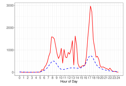
Figure A.1: Squared distance trajectory corresponding to 21 August 2017 (solid red) as compared against the overall Fréchet variance function (dashed blue).

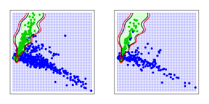
Figure A.2: Classification boundary of the support vector machine (black) and Bayes decision boundary (red), for the training data (left) and the test data (right).

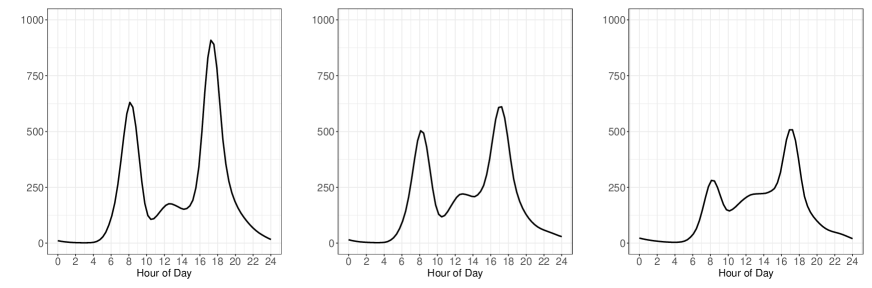
Figure A.3: Mean function $\frac{1}{n}\sum_{i=1}^{n}V_{i}(t)$ of the Fréchet variance trajectories of the time courses of daily Divvy bike trip networks in Chicago for weekdays (left), Fridays (middle) and weekends and holidays (right).

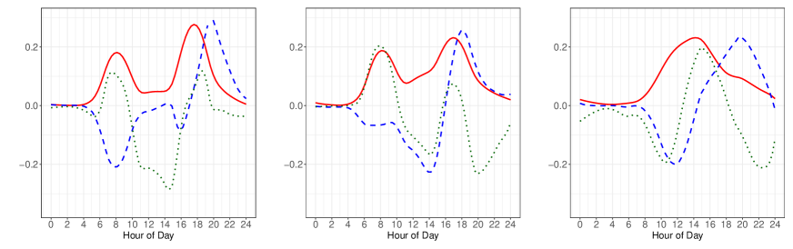
Figure A.4: Eigenfunctions corresponding to the FPCA of the daily Fréchet variance trajectories for weekdays (left), Fridays (middle) and weekends and holidays (right). The solid red line corresponds to the first, the dashed blue line to the second and the dotted green line to the third eigenfunction.

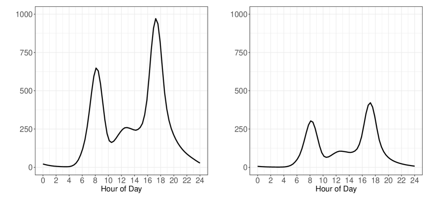
Figure A.5: Mean function $\frac{1}{n}\sum_{i=1}^{n}V_{i}(t)$ of the Fréchet variance trajectories of the time courses of daily Divvy bike trip networks in Chicago for Fridays in Spring, Summer and early Fall (left) and in late Fall and Winter (right).

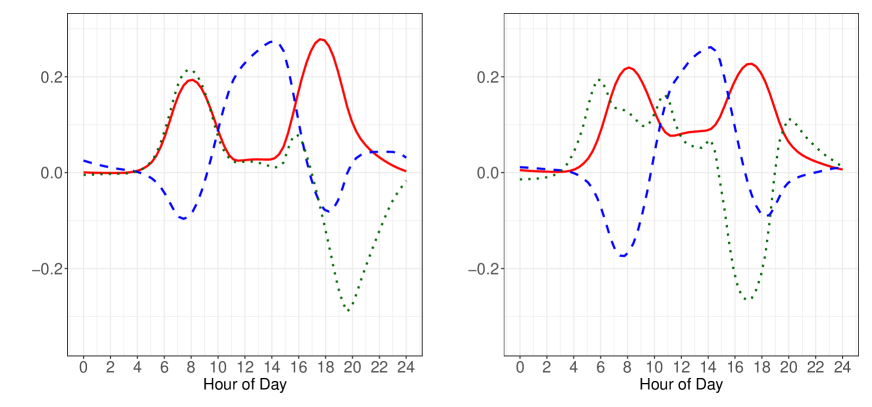
Figure A.6: Eigenfunctions corresponding to the FPCA of the daily Fréchet variance trajectories for spring, summer and early fall, Fridays (left) and late fall and winter (right). The solid red line corresponds to the first eigenfunction, the dashed blue line to the second and the dotted green line to the third eigenfunction.

A.5 Discussion on examples of $(\Omega,d)$ satisfying assumptions (A1)-(A5)

Distributions

Let $\Omega$ be the space of univariate probability distributions represented as quantile functions and let $d$ be the 2-Wasserstein metric. For quantile functions $Q_{1}(\cdot)$ and $Q_{2}(\cdot)$, the 2-Wasserstein metric is the $L_{2}$ metric is

$$d^{2}(Q_{1},Q_{2})=\int_{0}^{1}(Q_{1}(t)-Q_{2}(t))^{2}dt=||Q_{1}-Q_{2}||^{2}_{L_{2}}.$$

Let $Q_{X(s)}$ be the quantile function associated with the distribution of $X(s)$ for a fixed $s$ and $Q_{\omega}$ the quantile function associated with the distribution $\omega\in\Omega$. Then

$$E\{d^{2}(X(s),\omega)\}= E\{||Q_{X(s)}-Q_{\omega}||^{2}_{L_{2}}\}$$

$$= E\{\langle Q_{X(s)}-E(Q_{X(s)})+E(Q_{X(s)})-Q_{\omega},Q_{X(s)}-E(Q_{X(s)})+E(Q_{X(s)})-Q_{\omega}\rangle_{L_{2}}\}$$

$$= E\{\langle Q_{X(s)}-E(Q_{X(s)}),Q_{X(s)}-E(Q_{X(s)})\rangle_{L_{2}}\}+\langle E(Q_{X(s)})-Q_{\omega},E(Q_{X(s)})-Q_{\omega}\rangle_{L_{2}}$$

$$= E\{||Q_{X(s)}-E(Q_{X(s)})||^{2}_{L_{2}}\}+||E(Q_{X(s)})-Q_{\omega}||^{2}_{L_{2}}.$$

Therefore $Q_{\mu(s)}=\operatornamewithlimits{argmin}_{\omega\in\Omega}||E(Q_{X(s)})-Q_{\omega}||^{2}_{L_{2}}=E(Q_{X(s)})$ by the convexity of the space of quantile functions. In the sample version, let $\bar{Q}(s)(\cdot)=\frac{1}{n}\sum_{i=1}^{n}Q_{X_{i}(s)}(\cdot)$. The same algebra as above implies

$$\frac{1}{n}\sum_{i=1}^{n}d^{2}(X_{i}(s),\omega)=\frac{1}{n}\sum_{i=1}^{n}||Q_{X_{i}(s)}-\bar{Q}(s)||^{2}_{L_{2}}+||\bar{Q}(s)-Q_{\omega}||^{2}_{L_{2}},$$

whence $Q_{\hat{\mu}(s)}=\operatorname*{argmin}_{\omega\in\Omega}||\bar{Q}(s)-Q_{\omega}||^{2}_{L_{2}}=\bar{Q}(s)$ by the convexity of the space of quantile functions. Hence both $\mu(s)$ and $\hat{\mu}(s)$ exist and are unique as their quantile representations exist and are unique. Moreover, the above calculations also imply that

$$E\{d^{2}(X(s),\omega)\}-E\{d^{2}(X(s),\mu(s))\}=||Q_{\omega}-Q_{\mu(s)}||^{2}_{L_{2}}$$

and

$$\frac{1}{n}\sum_{i=1}^{n}d^{2}(X_{i}(s),\omega)-\frac{1}{n}\sum_{i=1}^{n}d^{2}(X_{i}(s),\hat{\mu}(s))=||Q_{\omega}-Q_{\hat{\mu}(s)}||^{2}_{L_{2}},$$

whence

$$\inf_{s\in[0,1]}\inf_{\,\omega\in\Omega:\,d(\omega,\mu(s))>\epsilon}E(d^{2}(X(s),\omega))-E(d^{2}(X(s),\mu(s)))>0.$$

Therefore (A1) holds with $\tau(\epsilon)=\epsilon^{2}$ and (A2) holds with $D=1$ and $\beta=2$, while (A4) is satisfied using the arguments in the proof of Proposition 1 of Petersen and Müller (2019).

Assumption (A3) is a common requirement for classical real-valued functional data, where trajectories are sometimes assumed to be twice differentiable with bounded second derivative. An example of time varying distributions is a sample of random density valued trajectories, where $X(t)$ is a normal distribution for all $t$. For an explicit sample construction, assume that the means of these normal distributions are $\mu(t)$ and the variances are $\sigma^{2}(t)$, both taken as random functions

$$\mu(t)=X_{1}+X_{2}\sin(2\pi t)\quad\text{and}\quad\sigma^{2}(t)=X_{3}e^{0.25t},$$

where $X_{1}$ and $X_{2}$ are independent uniform r.v.s in $[-1,1]$ and $X_{3}$ is an independent exponential r.v., with mean one, truncated to lie in $[0.25,3]$. Each $\omega(\cdot)$ in the sample space of trajectories is therefore a density valued process, where $\omega(s)$ is a normal distribution with mean of the form $a+b\sin{2\pi s}$, where $a,b\in[-1,1]$, and variance of the form $ce^{0.25s}$, where $c\in[0.25,3]$. For two univariate normal distributions, $f_{1}\sim N(\mu_{1},\sigma^{2}_{1})$ and $f_{2}\sim N(\mu_{2},\sigma^{2}_{2})$, the Wasserstein distance between $f_{1}$ and $f_{2}$ can be explicitly calculated as

$$d(f_{1},f_{2})=\sqrt{(\mu_{1}-\mu_{2})^{2}+(\sigma_{1}-\sigma_{2})^{2}},$$

which for the example above yields

$$d(X(s),X(t))=\sqrt{X_{2}^{2}(\sin(2\pi s)-\sin(2\pi t))^{2}+X_{3}^{2}(e^{0.25s}-e^{0.25t})^{2}}.$$ (27)

Condition (A3) is satisfied as both $\sin 2\pi t$ and $e^{0.25t}$ have bounded derivatives in $[0,1]$ and the second moments of $X_{1}$, $X_{2}$ and $X_{3}$ are finite.

Networks

Let $\Omega$ be the space of graph adjacency matrices or graph Laplacians of weighted networks, with uniformly bounded weights and let $d$ be the Frobenius metric. For matrices $U$ and $V$ the Frobenius metric is given by

$$d^{2}(U,V)=\sum_{i,j}(u_{ij}-v_{ij})^{2}=(U-V)^{T}(U-V).$$

For any $\omega\in\Omega$, by the properties of the Frobenius metric,

$$E\{d^{2}(X(s),\omega)\}= E\{(X(s)-\omega)^{T}(X(s)-\omega)\}$$

$$= E\{(X(s)-E(X(s))+E(X(s))-\omega)^{T}(X(s)-E(X(s))+E(X(s))-\omega)\}$$

$$= E\{(X(s)-E(X(s)))^{T}(X(s)-E(X(s)))\}+(E(X(s))-\omega)^{T}(E(X(s))-\omega)$$

$$= E\{d^{2}(X(s),E(X(s)))\}+d^{2}(E(X(s)),\omega).$$

Therefore $\mu(s)=\operatornamewithlimits{argmin}_{\omega\in\Omega}E\{d^{2}(X(s),\omega)\}$ = $\operatornamewithlimits{argmin}_{\omega\in\Omega}d^{2}(E(X(s)),\omega)=E(X(s))$ by the convexity of the space of graph Laplacians and adjacency matrices. In the sample version, let $\bar{X}(s)=\frac{1}{n}\sum_{i=1}^{n}X_{i}(s)$. By following the above algebra, one can show that

$$\frac{1}{n}\sum_{i=1}^{n}d^{2}(X_{i}(s),\omega)=\frac{1}{n}\sum_{i=1}^{n}d^{2}(X_{i}(s),\bar{X}(s))+d^{2}(\bar{X}(s),\omega),$$

which implies that $\hat{\mu}(s)=\operatorname*{argmin}_{\omega\in\Omega}\frac{1}{n}\sum_{i=1}^{n}d^{2}(X_{i}(s),\omega)=\operatorname*{argmin}_{\omega\in\Omega}d^{2}(\bar{X}(s),\omega)=\bar{X}(s)$, again by the convexity of the space of graph Laplacians and adjacency matrices. Hence both $\mu(s)$ and $\hat{\mu}(s)$ exist and are unique. Moreover, the above calculations imply that

$$E\{d^{2}(X(s),\omega)\}-E\{d^{2}(X(s),\mu(s))\}=d^{2}(\omega,\mu(s))$$

and

$$\frac{1}{n}\sum_{i=1}^{n}d^{2}(X_{i}(s),\omega)-\frac{1}{n}\sum_{i=1}^{n}d^{2}(X_{i}(s),\hat{\mu}(s))=d^{2}(\omega,\hat{\mu}(s)),$$

whence

$$\inf_{s\in[0,1]}\inf_{\,\omega\in\Omega:\,d(\omega,\mu(s))>\epsilon}E(d^{2}(X(s),\omega))-E(d^{2}(X(s),\mu(s)))>0$$

and therefore (A1) holds with $\tau(\epsilon)=\epsilon^{2}$ and (A2) holds with $D=1$ and $\beta=2$. As the graph adjacency matrices and graph Laplacians of networks with bounded edge connectivities form a subset of a larger finite-dimensional bounded Euclidean space, (A4) is also satisfied using the arguments in the proof of Proposition 2 of Petersen and Müller (2019).

In our example of graph Laplacians or graph adjacencies of weighted networks with a fixed number of nodes, assumption (A3) on Hölder continuity translates into Hölder equicontinuity of the individual edge connectivities. For an example of a practical data generating model that satisfies this criterion, assume that the network adjacency matrix $X(t)$ is generated as

$$\{X(t)\}_{k,l}=W_{kl}(t)\left\{\frac{1+\sin(V_{kl}\pi(t+U_{kl}))}{2}\right\},$$

where $W_{kl}(t)$ is a smooth weight function with bounded derivatives, $U_{kl}$ is generated independently from $U(0,1)$ and $V_{kl}$ is generated uniformly from $\{1,2,\dots,10\}$. Here $U_{kl}$ and $V_{kl}$ are the random phase and frequency shift of the sine function which controls where in the time domain and how many times the edge connectivity $\{X(t)\}_{k,l}$ hits zero, in which case there is no link between nodes $k$ and $l$. Each network in the sample space, with adjacency matrix $\omega(t)$, is of the form

$$\{\omega(t)\}_{k,l}=W_{kl}(t)\left\{\frac{1+\sin(v\pi(t+u))}{2}\right\}.$$

Therefore all the networks in the sample space satisfy assumption (A3). We also adopt this construction as a data generating model in our simulations.

REFERENCES

- Agostinelli (2018) Agostinelli, C. (2018), “Local half-region depth for functional data,” Journal of Multivariate Analysis, 163, 67–79.
- Ahidar-Coutrix et al. (2020) Ahidar-Coutrix, A., Le Gouic, T., and Paris, Q. (2020), “Convergence rates for empirical barycenters in metric spaces: curvature, convexity and extendable geodesics,” Probability theory and related fields, 177, 323–368.
- Anirudh et al. (2017) Anirudh, R., Turaga, P., Su, J., and Srivastava, A. (2017), “Elastic functional coding of Riemannian trajectories,” IEEE Transactions on Pattern Analysis and Machine Intelligence, 39, 922–936.
- Arribas-Gil and Romo (2014) Arribas-Gil, A. and Romo, J. (2014), “Shape outlier detection and visualization for functional data: the outliergram,” Biostatistics, 15, 603–619.
- Berrendero et al. (2011) Berrendero, J., Justel, A., and Svarc, M. (2011), “Principal components for multivariate functional data,” Computational Statistics and Data Analysis, 55, 2619–2634.
- Bhattacharya and Patrangenaru (2003) Bhattacharya, R. and Patrangenaru, V. (2003), “Large sample theory of intrinsic and extrinsic sample means on manifolds - I,” Annals of Statistics, 31, 1–29.
- Bigot et al. (2018) Bigot, J., Cazelles, E., and Papadakis, N. (2018), “Data-driven regularization of Wasserstein barycenters with an application to multivariate density registration,” arXiv preprint arXiv:1804.08962.
- Bolstad et al. (2003) Bolstad, B. M., Irizarry, R., Åstrand, M., and Speed, T. (2003), “A comparison of normalization methods for high density oligonucleotide array data based on variance and bias,” Bioinformatics, 19, 185–193.
- Bosq (2000) Bosq, D. (2000), Linear Processes in Function Spaces: Theory and Applications, New York: Springer-Verlag.
- Calhoun et al. (2014) Calhoun, V. D., Miller, R., Pearlson, G., and Adali, T. (2014), “The chronnectome: time-varying connectivity networks as the next frontier in fMRI data discovery,” Neuron, 84, 262–274.
- Castro et al. (1986) Castro, P. E., Lawton, W. H., and Sylvestre, E. A. (1986), “Principal modes of variation for processes with continuous sample curves,” Technometrics, 28, 329–337.
- Chen et al. (2017) Chen, K., Delicado, P., and Müller, H.-G. (2017), “Modeling function-valued stochastic processes, with applications to fertility dynamics,” Journal of the Royal Statistical Society, Series B (Theory and Methodology), 79, 177–196.
- Chen and Lei (2015) Chen, K. and Lei, J. (2015), “Localized functional principal component analysis,” Journal of the American Statistical Association, 110, 1266–1275.
- Chiou and Li (2007) Chiou, J.-M. and Li, P.-L. (2007), “Functional clustering and identifying substructures of longitudinal data,” Journal of the Royal Statistical Society: Series B, 69, 679–699.
- Ciollaro et al. (2016) Ciollaro, M., Genovese, C. R., and Wang, D. (2016), “Nonparametric clustering of functional data using pseudo-densities,” Electronic Journal of Statistics, 10, 2922–2972.
- Dai et al. (2020) Dai, X., Lin, Z., and Müller, H.-G. (2020), “Modeling sparse longitudinal data on Riemannian manifolds,” Biometrics (to appear).
- Dai and Müller (2018) Dai, X. and Müller, H.-G. (2018), “Principal Component Analysis for Functional Data on Riemannian Manifolds and Spheres,” Annals of Statistics, 46, 3334–3361.
- Dosman et al. (2012) Dosman, C. F., Andrews, D., and Goulden, K. J. (2012), “Evidence-based milestone ages as a framework for developmental surveillance,” Paediatrics & child health, 17, 561–568.
- Dryden (2012) Dryden, I. (2012), “Shapes package,” R Package Version, 1.
- Dryden and Mardia (2016) Dryden, I. L. and Mardia, K. V. (2016), Statistical shape analysis: with applications in R, vol. 995, John Wiley & Sons.
- Dubey and Müller (2019a) Dubey, P. and Müller, H.-G. (2019a), “Fréchet analysis of variance for random objects,” Biometrika, 106, 803–821.
- Dubey and Müller (2019b) — (2019b), “Functional models for time-varying random objects,” arXiv preprint arXiv:1907.10829 Journal of the Royal Statistical Society B, to appear.
- Durrleman et al. (2013) Durrleman, S., Pennec, X., Trouvé, A., Braga, J., Gerig, G., and Ayache, N. (2013), “Toward a comprehensive framework for the spatiotemporal statistical analysis of longitudinal shape data,” International Journal of Computer Vision, 103, 22–59.
- Febrero et al. (2008) Febrero, M., Galeano, P., and González-Manteiga, W. (2008), “Outlier detection in functional data by depth measures, with application to identify abnormal NOx levels,” Environmetrics, 19, 331–345.
- Ferraty et al. (2007) Ferraty, F., Mas, A., and Vieu, P. (2007), “Nonparametric regression on functional data: inference and practical aspects,” Australian and New Zealand Journal of Statistics, 49, 459–461.
- Fieuws and Verbeke (2006) Fieuws, S. and Verbeke, G. (2006), “Pairwise fitting of mixed models for the joint modeling of multivariate longitudinal profiles,” Biometrics, 62, 424–431.
- Fitzmaurice et al. (2008) Fitzmaurice, G., Davidian, M., Verbeke, G., and Molenberghs, G. (2008), Longitudinal data analysis, CRC Press.
- Fréchet (1948) Fréchet, M. (1948), “Les éléments aléatoires de nature quelconque dans un espace distancié,” Annales de l’Institut Henri Poincaré, 10, 215–310.
- Gasser et al. (1984) Gasser, T., Müller, H.-G., Köhler, W., Molinari, L., and Prader, A. (1984), “Nonparametric Regression Analysis of Growth Curves,” Annals of Statistics, 12, 210–229.
- Gervini and Khanal (2019) Gervini, D. and Khanal, M. (2019), “Exploring patterns of demand in bike sharing systems via replicated point process models,” Journal of the Royal Statistical Society Series C: Applied Statistics, 68, 585–602.
- Guo (2004) Guo, W. (2004), “Functional data analysis in longitudinal settings using smoothing splines,” Statistical Methods in Medical Research, 13, 49–62.
- Hall and Hosseini-Nasab (2006) Hall, P. and Hosseini-Nasab, M. (2006), “On properties of functional principal components analysis,” Journal of the Royal Statistical Society: Series B, 68, 109–126.
- Hall and Van Keilegom (2007) Hall, P. and Van Keilegom, I. (2007), “Two-sample tests in functional data analysis starting from discrete data,” Statistica Sinica, 1511–1531.
- Horvath and Kokoszka (2012) Horvath, L. and Kokoszka, P. (2012), Inference for Functional Data with Applications, New York: Springer.
- Hsing and Eubank (2015) Hsing, T. and Eubank, R. (2015), Theoretical Foundations of Functional Data Analysis, with an Introduction to Linear Operators, John Wiley & Sons.
- Huisman and Snijders (2003) Huisman, M. and Snijders, T. A. (2003), “Statistical analysis of longitudinal network data with changing composition,” Sociological Methods & Research, 32, 253–287.
- Jacques and Preda (2014) Jacques, J. and Preda, C. (2014), “Model-based clustering for multivariate functional data,” Computational Statistics and Data Analysis, 71, 92–106.
- Kendall (1984) Kendall, D. G. (1984), “Shape manifolds, procrustean metrics, and complex projective spaces,” Bulletin of the London mathematical society, 16, 81–121.
- Kendall (1989) — (1989), “A survey of the statistical theory of shape,” Statistical Science, 87–99.
- Kleffe (1973) Kleffe, J. (1973), “Principal components of random variables with values in a separable Hilbert space,” Mathematische Operationsforschung und Statistik, 4, 391–406.
- Kossinets and Watts (2006) Kossinets, G. and Watts, D. J. (2006), “Empirical analysis of an evolving social network,” science, 311, 88–90.
- Le (1995) Le, H. (1995), “Mean size-and-shapes and mean shapes: a geometric point of view,” Advances in Applied Probability, 27, 44–55.
- Le (1998) — (1998), “On the consistency of procrustean mean shapes,” Advances in Applied Probability, 53–63.
- Le and Kendall (1993) Le, H. and Kendall, D. G. (1993), “The Riemannian structure of Euclidean shape spaces: a novel environment for statistics,” The annals of Statistics, 1225–1271.
- Li and Guan (2014) Li, Y. and Guan, Y. (2014), “Functional principal component analysis of spatiotemporal point processes with applications in disease surveillance,” Journal of the American Statistical Association, 109, 1205–1215.
- Lila and Aston (2019) Lila, E. and Aston, J. A. (2019), “Statistical Analysis of Functions on Surfaces, with an application to Medical Imaging,” Journal of the American Statistical Association.
- Lin et al. (2020) Lin, Z., Shao, L., and Yao, F. (2020), “Intrinsic Riemannian Functional Data Analysis for Sparse Longitudinal Observations,” arXiv preprint arXiv:2009.07427.
- Lin et al. (2016) Lin, Z., Wang, L., and Cao, J. (2016), “Interpretable functional principal component analysis,” Biometrics, 72, 846–854.
- Liu and Müller (2009) Liu, B. and Müller, H.-G. (2009), “Estimating derivatives for samples of sparsely observed functions, with application to on-line auction dynamics.” Journal of the American Statistical Association, 104, 704–714.
- López-Pintado and Romo (2009) López-Pintado, S. and Romo, J. (2009), “On the concept of depth for functional data,” Journal of the American Statistical Association, 104, 718–734.
- Mardia et al. (2005) Mardia, K. V., Patrangenaru, V., et al. (2005), “Directions and projective shapes,” The Annals of Statistics, 33, 1666–1699.
- Mas and Pumo (2009) Mas, A. and Pumo, B. (2009), “Functional linear regression with derivatives,” Journal of Nonparametric Statistics, 21, 19–40.
- Müller and Yao (2010) Müller, H.-G. and Yao, F. (2010), “Empirical dynamics for longitudinal data,” Annals of Statistics, 38, 3458–3486.
- Muralidharan and Fletcher (2012) Muralidharan, P. and Fletcher, P. T. (2012), “Sasaki metrics for analysis of longitudinal data on manifolds,” in Computer Vision and Pattern Recognition (CVPR), 2012 IEEE Conference on, IEEE, pp. 1027–1034.
- Nagy and Ferraty (2019) Nagy, S. and Ferraty, F. (2019), “Data depth for measurable noisy random functions,” Journal of Multivariate Analysis, 170, 95–114.
- Nagy et al. (2017) Nagy, S., Gijbels, I., and Hlubinka, D. (2017), “Depth-based recognition of shape outlying functions,” Journal of Computational and Graphical Statistics, 26, 883–893.
- Nie et al. (2017) Nie, Y., Wang, L., and Cao, J. (2017), “Estimating time-varying directed gene regulation networks,” Biometrics.
- Ossiander (1987) Ossiander, M. (1987), “A Central Limit Theorem under metric entropy with bracketing,” The Annals of Probability, 15, 897–919.
- Patrangenaru and Ellingson (2015) Patrangenaru, V. and Ellingson, L. (2015), Nonparametric Statistics on Manifolds and Their Applications to Object Data Analysis, CRC Press.
- Patrangenaru et al. (2016a) Patrangenaru, V., Guo, R., and Yao, K. D. (2016a), “Nonparametric inference for location parameters via Fréchet functions,” in 2016 Second International Symposium on Stochastic Models in Reliability Engineering, Life Science and Operations Management (SMRLO), IEEE, pp. 254–262.
- Patrangenaru et al. (2016b) Patrangenaru, V., Yao, K. D., and Guo, R. (2016b), “Extrinsic means and antimeans,” in Nonparametric Statistics, Springer, pp. 161–178.
- Petersen and Müller (2019) Petersen, A. and Müller, H.-G. (2019), “Fréchet regression for random objects with Euclidean predictors,” Annals of Statistics, 47, 691–719.
- Ramsay (2000) Ramsay, J. (2000), “Differential equation models for statistical functions,” Cnadian Journal of Statistics, 28, 225–240.
- Ramsay et al. (2007) Ramsay, J. O., Hooker, G., Campbell, D., and Cao, J. (2007), “Parameter Estimation for Differential Equations: A Generalized Smoothing Approach (with discussion),” Journal of the Royal Statistical Society: Series B, 69, 741–796.
- Ramsay and Silverman (2005) Ramsay, J. O. and Silverman, B. W. (2005), Functional Data Analysis, Springer Series in Statistics, New York: Springer, 2nd ed.
- Ren et al. (2017) Ren, H., Chen, N., and Zou, C. (2017), “Projection-based outlier detection in functional data,” Biometrika, 104, 411–423.
- Rice (2004) Rice, J. A. (2004), “Functional and longitudinal data analysis: Perspectives on smoothing,” Statistica Sinica, 631–647.
- Romano and Mateu (2013) Romano, E. and Mateu, J. (2013), “Outlier detection for geostatistical functional data: an application to sensor data,” in Classification and Data Mining, Springer, pp. 131–138.
- Schiratti et al. (2015) Schiratti, J.-B., Allassonniere, S., Colliot, O., and Durrleman, S. (2015), “Learning spatiotemporal trajectories from manifold-valued longitudinal data,” in Advances in Neural Information Processing Systems, pp. 2404–2412.
- Sentürk and Müller (2010) Sentürk, D. and Müller, H.-G. (2010), “Functional varying coefficient models for longitudinal data,” Journal of the American Statistical Association, 105, 1256–1264.
- Snijders (2005) Snijders, T. A. (2005), “Models for longitudinal network data,” Models and methods in social network analysis, 1, 215–247.
- Sturm (2003) Sturm, K.-T. (2003), “Probability measures on metric spaces of nonpositive curvature,” Heat Kernels and Analysis on Manifolds, Graphs, and Metric Spaces (Paris, 2002). Contemp. Math., 338. Amer. Math. Soc., Providence, RI, 357–390.
- Suarez and Ghosal (2016) Suarez, A. J. and Ghosal, S. (2016), “Bayesian clustering of functional data using local features,” Bayesian Analysis, 11, 71–98.
- Tarpey and Kinateder (2003) Tarpey, T. and Kinateder, K. K. (2003), “Clustering functional data,” Journal of Classification, 20, 093–114.
- Van der Vaart and Wellner (1996) Van der Vaart, A. and Wellner, J. (1996), Weak Convergence and Empirical Processes, Springer, New York.
- Verbeke et al. (2014) Verbeke, G., Fieuws, S., Molenberghs, G., and Davidian, M. (2014), “The analysis of multivariate longitudinal data: A review,” Statistical Methods in Medical Research, 23, 42–59.
- Wang et al. (2016) Wang, J.-L., Chiou, J.-M., and Müller, H.-G. (2016), “Functional Data Analysis,” Annual Review of Statistics and its Application, 3, 257–295.
- Wang et al. (2020) Wang, Y., Patrangenaru, V., and Guo, R. (2020), “A Central Limit Theorem for extrinsic antimeans and estimation of Veronese-Whitney means and antimeans on planar Kendall shape spaces,” Journal of Multivariate Analysis, 104600.
- Xiang et al. (2013) Xiang, D., Qiu, P., and Pu, X. (2013), “Nonparametric regression analysis of multivariate longitudinal data,” Statistica Sinica, 23, 769–789.
- Yang et al. (2007) Yang, X., Shen, Q., Xu, H., and Shoptaw, S. (2007), “Functional regression analysis using an F test for longitudinal data with large numbers of repeated measures,” Statistics in Medicine, 26, 1552–1566.
- Zhang and Chen (2007) Zhang, J.-T. and Chen, J. (2007), “Statistical inferences for functional data,” The Annals of Statistics, 35, 1052–1079.
- Zhou et al. (2008) Zhou, L., Huang, J., and Carroll, R. (2008), “Joint modelling of paired sparse functional data using principal components,” Biometrika, 95, 601–619.