Inferring Risks of Coronavirus Transmission from Community Household Data

Abstract

The response of many governments to the COVID-19 pandemic has involved measures to control within- and between-household transmission, providing motivation to improve understanding of the absolute and relative risks in these contexts. Here, we perform exploratory, residual-based, and transmission-dynamic household analysis of the Office for National Statistics (ONS) COVID-19 Infection Survey (CIS) data from 26 April 2020 to 15 July 2021 in England. This provides evidence for: (i) temporally varying rates of introduction of infection into households broadly following the trajectory of the overall epidemic and vaccination programme; (ii) Susceptible-Infectious Transmission Probabilities (SITPs) of within-household transmission in the 15-35% range; (iii) the emergence of the Alpha and Delta variants, with the former being around 50% more infectious than wildtype and 35% less infectious than Delta within households; (iv) significantly (in the range 25-300%) more risk of bringing infection into the household for workers in patient-facing roles pre-vaccine; (v) increased risk for secondary school-age children of bringing the infection into the household when schools are open; (vi) increased risk for primary school-age children of bringing the infection into the household when schools were open since the emergence of new variants.

1 Introduction

1.1 Analysis of household infection data

Households have often played an important role in infectious disease epidemiology, with policies in place and under consideration in the UK to reduce both within- and between-household transmission (Scientific Advisory Group for Emergencies, 2021). This is because the close, repeated nature of contact within the household means that within-household transmission of infectious disease is common. Also, most of the population lives in relatively small, stable households (Office for National Statistics, 2019). From the point of view of scientific research, the household is a natural unit for epidemiological data collection and households are small enough to allow for explicit solution of relatively complex transmission models. Some of the earliest work in this field was carried out by Reed and Frost, whose model was first described in the literature by Abbey (1952) in a paper that analysed transmission in boarding schools and other closed populations. Frost’s 1928 lecture was later published posthumously (Frost, 1976), with a re-analysis of his original household dataset from the 1918 influenza pandemic carried out using modern computational and modelling approaches by Fraser et al. (2011).

Subsequent important contributions were made in empirical studies of transmission in households, for example the highly influential study of childhood diseases by Hope Simpson (1952), and epidemic theory based on the analyses of discrete- and continuous-time Markovian epidemics presented by Bailey (1957). A key development was the solution by Ball (1986) of the final size distribution of a random epidemic in a household without requiring Markovian recovery from infection, which then enabled statistical analyses of household infection data such as that by Addy et al. (1991). Still further progress is possible due to the use of modern computational methods, particularly Monte Carlo approaches, to augment datasets (O’Neill and Roberts, 1999; Cauchemez et al., 2004; Demiris and O’Neill, 2005) or to avoid likelihood calculations (Neal, 2012).

Continued methodological developments and data availability have enabled increasingly sophisticated inferences to be drawn from household studies of respiratory pathogens, dealing with for example interactions between adults and children (van Boven et al., 2010), case ascertainment (House et al., 2012), interactions between strains (Kombe et al., 2019), and details of family structure (Endo et al., 2019). During the current pandemic, there have been numerous household studies (Madewell et al., 2020), with three recently published studies being notable for combining fitting of a transmission model with significant differentiation of risks being those of Dattner et al. (2021), Li et al. (2021) and Reukers et al. (2021).

1.2 Context for this study

The severe acute respiratory syndrome coronavirus 2 (SARS-CoV-2) emerged in the human population in late 2019 and the WHO declared a pandemic in March 2020 (World Health Organization, 2020). Early in the pandemic, it became clear that risks of transmission, mortality and morbidity from the associated coronavirus disease (COVID-19) were highly heterogeneous with age (Davies et al., 2020), and also that work in patient-facing roles was associated with increased risk of positivity in the community (Pouwels et al., 2021) as would be expected given the risks of healthcare-associated transmission (Bhattacharya et al., 2021).

During the period of the study, there have been two major ‘sweeps’ in the UK, during which a SARS-CoV-2 variant of concern (VOC) emerged and became dominant.

The first of these was PANGO lineage B.1.1.7 (Rambaut et al., 2020b), or ‘Alpha’ under WHO nomenclature (World Health Organization, 2021). The first samples of this variant were found in September 2020 (Rambaut et al., 2020b), and it was designated a VOC on 18 December 2020 (Public Health England, 2021c). There is evidence for both increased transmissibility of this variant, and increased mortality amongst infected cases (Davies et al., 2021; Challen et al., 2021; Grint et al., 2021), although conditional on hospitalisation outcomes may not be worse (Frampton et al., 2021). The second VOC to emerge was PANGO lineage B.1.617.2 (Rambaut et al., 2020a), or ‘Delta’ under WHO nomenclature (World Health Organization, 2021), which was designated a VOC on 6 May 2021 and is at time of writing the dominant variant in the UK (Public Health England, 2021b).

Both of these variants were relatively easy to track through the S gene target in commonly-used polymerase chain reaction (PCR) tests, with more details on this approach provided in §2.1 below.

Throughout 2021, the UK rolled out a comprehensive vaccination programme with priority given to healthcare workers, the clinically vulnerable, and then with prioritisation by age, from oldest to youngest (Office for National Statistics, 2021; Public Health England, 2021a). We will not include vaccination here at the individual level, but rather note its overall effect on infection and transmission at different times.

Here, we apply a combination of methods, including a regression that explicitly accounts for transmission, to the Office for National Statistics (ONS) COVID-19 Infection Survey (CIS) data from 26 April 2020 to 15 July 2021 (Pouwels et al., 2021). We particularly consider the absolute magnitude of transmission within and between households, as well as the associations between these and household size, age, infection with VOCs (inferred via S gene target) and work in patient-facing roles.

2 Methods

2.1 Description of data

ONS CIS has a design based on variable levels of recruitment by region and time as required by policy, but otherwise uniformly random selection of households from address lists and previous ONS studies on an ongoing basis. If verbal agreement to participate is obtained, a study worker visits each household to take written informed consent, which is obtained from parents/carers for those aged 2-15 years. Participants aged 10-15 years provide written assent and those under 2 years old are not eligible.

Participants are asked questions on issues including work and age as well as being tested for SARS-CoV-2 infection via reverse transcription PCR (RT-PCR). To reduce transmission risks, participants aged 12 years and over self-collect nose and throat swabs following study worker instructions, and parents/carers take swabs from children aged under 12 years. At the first visit, participants are asked for optional consent for follow-up visits every week for the next month, then monthly for 12 months from enrolment. The first few weeks of a hypothetical household participating in this study are shown schematically in Figure 1.

Swabs were analysed at the UK’s national Lighthouse Laboratories at Milton Keynes and Glasgow using identical methodology. RT-PCR for three SARS-CoV-2 genes (N protein, S protein and ORF1ab) used the Thermo Fisher TaqPath RT-PCR COVID-19 Kit, and analysed using UgenTec FastFinder 3.300.5, with an assay-specific algorithm and decision mechanism that allows conversion of amplification assay raw data from the ABI 7500 Fast into test results with minimal manual intervention. Samples are called positive if at least a single N-gene and/or ORF1ab are detected. Although S gene cycle threshold (Ct) values are determined, S gene detection alone is not considered sufficient to call a sample positive.

This analysis includes all SARS-CoV-2 RT-PCR tests of nose and throat swabs from 26 April 2020 to 15 July 2021 for English households in the ONS CIS. We restrict our analysis to households of size 6 and under, partly for computational reasons that we will discuss below, and partly because this captures the overwhelming majority of households, with larger households being atypical in various ways (Office for National Statistics, 2019). Over 94% of households have all members participating, and for the remainder we treat the household as composed of participants only. In contrast to other studies, the households we select constitute an approximately representative sample from the population when stratified by date and region. The restriction to England was chosen because we split the data into four time periods, corresponding to changing situations about policies that are devolved (i.e. policies are different in Scotland, Wales and Northern Ireland). These time periods split the data into the following tranches, with associated time periods and notable events (described broadly).

• Tranche 1: 26 April 2020 to 31 August 2020; low prevalence; schools closed; Alpha and Delta variants not emerged yet; no vaccine available.

• Tranche 2: 1 September 2020 to 14 November 2020; high prevalence; schools open; negligible Alpha variant; Delta variant not emerged yet; no vaccine available.

• Tranche 3: 15 November 2020 to 31 December 2020; high prevalence; schools open; Alpha variant becomes dominant; Delta variant not emerged yet; negligible vaccine coverage.

• Tranche 4: 1 January 2021 to 14 February 2021; high prevalence; schools closed (except for pre-school); Alpha variant dominant; Delta variant not emerged yet; over 10 million first vaccine doses by end of time period.

• Tranche 5: 15 February 2021 to 29 April 2021; low prevalence; schools open; Delta variant negligible; over 35 million first and 15 million second vaccine doses by end of time period.

• Tranche 6: 30 April 2021 to 15 July 2021; high prevalence; schools open; Delta variant becomes dominant; over 45 million first and 35 million second doses distributed by end of time period.

These properties are summarised again in Table 1. The properties of the data allocated to these tranches are shown in Table 2. Note that, while we do not include new primary infections in households after 15 July 2021, but do include later secondary infections in households where the primary infection happened before 15 July 2021. This is done to reduce problems with censoring.

2.2 Mathematical representation of data

Suppose we have a set of $n$ individuals (participants), indexed $i,j,\ldots\in[n]$, where we use the notation $[k]$ to stand for the set of integers from $1$ to $k$ inclusive. These individuals are members of $m$ households, and we represent the $a$-th household using a set of individual indices $H_{a}$. These are specified such that each individual is in exactly one household, so formally,

$$H_{a}\subseteq[n],\forall a\in[m]\text{ ,}\quad H_{a}\cap H_{b}=\varnothing,\forall a\in[m],b\in[m]\setminus\{a\}\text{ ,}\quad\bigcup_{a=1}^{m}H_{a}=[n]\text{ .}$$

The size of the $a$-th household is then $n_{a}=|H_{a}|$. The $a$-th household is visited at a set of times $\mathcal{T}_{a}$, and for each $t\in\mathcal{T}_{a}$ we let $\mathbf{x}_{i,t}$ be the length-$p$ feature vector (also called covariates) associated with the $i$-th individual at time $t$, and $y_{i,t}$ be the test result so that $y_{i,t}=1$ if the swab is positive and $y_{i,t}=0$ if not. Note that not all $i\in H_{a}$ will register a valid observation for features and swab results for each $t\in\mathcal{T}_{a}$.

We let a tranche be defined by a time interval $T=[t_{1},t_{2})$, and the household $H_{a}$ will appear in the analysis associated with the tranche $T$ if $\mathcal{T}_{a}\cap T\neq\varnothing$. For the analysis that we will perform, we require a method for associating a unique positivity and feature vector with each individual for the duration of the tranche. Under our modelling assumptions, the following definition of tranche positivity is most natural. For each household $H_{a}$ associated with tranche $T$,

$$\forall i\in H_{a}\text{ ,}\quad y_{i}=\begin{cases}1&\text{ if }\exists t,y_{i,t}=1\ \&\ \min\{\tau|\exists j\in H_{a},y_{j,\tau}=1\}\in T\text{ ,}\\ 0&\text{ otherwise.}\end{cases}$$ (1)

This means that we associate every positive in the household with the tranche in which the first positive appears in that household. Such an approach would need revision for a situation where individuals were infected a large number of times (i.e. common reinfection) or if incidence were so high that a significant number of households would be expected to have multiple introductions, but we do not see these scenarios in our data. For features, the appropriate rule will depend on the feature. An example such rule for the case where there is only one feature $x_{i,t}\in\{0,1\},\forall i,t$ would be

$$x_{i}=\max\{x_{i,t}|t\in\mathcal{T}_{a}\cap T\}\text{ ,}$$

i.e. we take this feature to be $1$ if it is measured as $1$ at any point during the tranche in question.

2.3 Exploratory analysis of density and ages

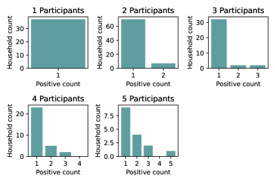
(a) Tranche 1

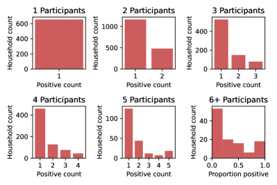
(b) Tranche 2

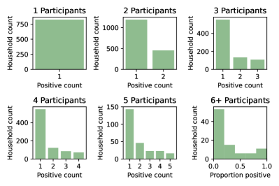
(c) Tranche 3

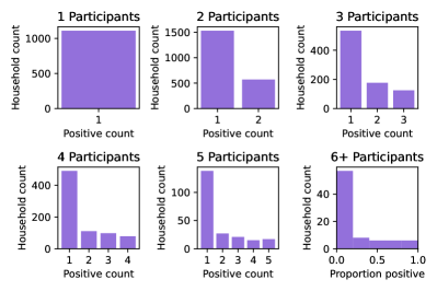
(d) Tranche 4

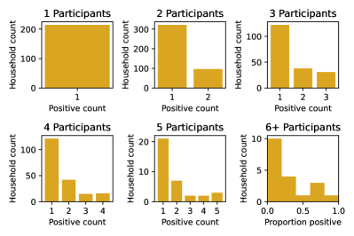
(e) Tranche 5

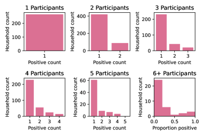
(f) Tranche 6

Figure 2: Histograms of household attack rates

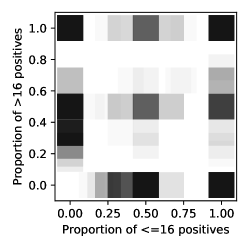
(d) Tranche 4

(e) Tranche 5

(f) Tranche 6

(g) Legend

Figure 3: Kernel density plots showing proportion of positives in different age classes in households.

An important part of our analysis will be consideration of counts / proportions of households with a given composition of cases displayed as histograms as in Figure 2, and density plots as in Figure 3.

The heights of the histogram bars are given by

$$Z_{k,\ell}=\sum_{a=1}^{m}\mathbb{1}_{\{n_{a}=\ell\}}\mathbb{1}_{\{\sum_{i\in H_{a}}y_{i}=k\}}\text{ ,}\quad\ell\in\{2,3,4,5,6\}\text{ ,}\quad k\in\{0,\ldots,\ell\}\text{ ,}$$

where $\mathbb{1}$ stands for the indicator function. Verbally, $Z_{k,\ell}$ is the count of households of size $\ell$ with $k$ participants testing positive.

The density plots are obtained by considering some feature (in this case, age) that takes values $0$ or $1$. We then form a point $\mathbf{r}_{a}\in[0,1]^{2}$ for each household $H_{a}$ such that

$$\sum_{i\in H_{a}}\mathbb{1}_{\{y_{i}=1\}}>0\text{ ,}\quad\sum_{i\in H_{a}}\mathbb{1}_{\{x_{i}=1\}}>0\text{ ,}\quad\sum_{i\in H_{a}}\mathbb{1}_{\{x_{i}=0\}}>0\text{ ,}$$

through the definition

$$\mathbf{r}_{a}=\left(\frac{\sum_{i\in H_{a}}\mathbb{1}_{\{y_{i}=1\&x_{i}=1\}}}{\sum_{i\in H_{a}}\mathbb{1}_{\{x_{i}=1\}}},\frac{\sum_{i\in H_{a}}\mathbb{1}_{\{y_{i}=1\&x_{i}=0\}}}{\sum_{i\in H_{a}}\mathbb{1}_{\{x_{i}=0\}}}\right)\text{ .}$$

Then we can construct a kernel density estimate in the usual way by summing then normalising kernel functions around the points, in particular the width-$w$ square kernel function

$$\mathcal{K}(\mathbf{r},\mathbf{r}_{a})=\mathbb{1}_{\{||\mathbf{r}-\mathbf{r}_{a}||_{\infty}<w\}}\text{ .}$$

We use age (16 years old and under versus over 16 years old) as the feature in making the density plots in Figure 3.

2.4 Residual analysis and gene positivity pattern

We are also interested in tabulation of features and positives in households in a manner that allows their clustering to be assessed. In particular, this involves calculation of Pearson residuals for the within-household pairs of features and positives. Let $x_{i}$ be the feature for individual $i$ that takes values with generic labels $A,B,\ldots$ (here mainly patterns of PCR target positivity and negativity indicative of viral strain). We are then interested in the table of pairs of individuals in households in the set $\mathcal{H}\subseteq[m]$ with certain properties,

$$Y_{AB}=\sum_{a\in\mathcal{H},i\in H_{a},j\in H_{a}\setminus\{i\}}\mathbb{1}_{\{x_{i}=A\}}\mathbb{1}_{\{x_{j}=B\}}\text{ .}$$

Verbally, $Y_{AB}$ is the count in the sample of $A$-$B$ pairs of distinct individuals in households from the set of households under consideration. On its own, this does not indicate whether $A$ and $B$ are more strongly associated with each other in households than would be expected from their overall prevalence in the household population. If we let

$$z_{A}=\sum_{a\in\mathcal{H},i\in H_{a}}\mathbb{1}_{\{x_{i}=A\}}\text{ ,}$$

then under the null hypothesis of independence, $\hat{\pi}_{A}=z_{A}/|\mathcal{H}|$ is the maximum likelihood estimator for the population probability of being in state $A$ and we can then construct an ‘expected’ table corresponding to each household pair having independent state with elements

$$E_{AB}=\hat{\pi}_{A}\hat{\pi}_{B}\sum_{a\in\mathcal{H}}n_{a}(n_{a}-1)\text{ .}$$

The Pearson residual associated with the $(A,B)$-th table entry is then

$$R_{AB}=\frac{Y_{AB}-E_{AB}}{\sqrt{E_{AB}}}\text{ .}$$ (2)

In simpler contexts, such residuals are typically asymptotically standard normal under the null hypothesis (Bishop et al., 1975). For our case, this simple result does not follow straightforwardly, but if we consider a sampled household $H$, let $X_{i}$ be the random variable state of the $i$-th household member, and let

$$Z_{A}=\sum_{i\in H}\mathbb{1}_{\{X_{i}=A\}}\text{ ,}$$

then the moment generating function for the random vector $\mathbf{Z}=(Z_{A})$ under the assumption of independence will be the multinomial

$$M_{\mathbf{Z}}(\mathbf{t})=\left(\sum_{A}\pi_{A}{\rm e}^{t_{A}}\right)^{|H|}\text{ .}$$

We can then calculate moments of the distribution of pairs through differentiation of this function, for example

$$\mathbb{E}\left[Z_{A}\left(Z_{B}-\mathbb{1}_{\{A=B\}}\right)\right]=\left.\frac{\partial^{2}M}{\partial t_{A}\partial t_{B}}\right|_{\mathbf{t}=\mathbf{0}}=\pi_{A}\pi_{B}n(n-1)\text{ .}$$

And so we can see that $R_{AB}$ as in (2) will be $0$ where there is no correlation between states at the household level. While explicit calculation of $\mathrm{Var}(Z_{A}(Z_{B}-\mathbb{1}_{\{A=B\}}))$ to determine its asymptotic distribution in the case of many households is beyond the scope of the current work, we believe that this would be an interesting direction for future study. Nevertheless, due to the arguments presented above we can interpret larger values of $R_{AB}$ as indicative of more positive correlation between states at the household level and vice versa.

Here we will use pattern of PCR target failure as a feature and the restriction of households to those in which there is at least one infection (to avoid domination of the tables by all-negative households), i.e.

$$\mathcal{H}=\bigg{\{}a\in[m]\;\bigg{|}\;\sum_{i\in H_{a}}y_{i}>0\bigg{\}}\text{ ,}$$

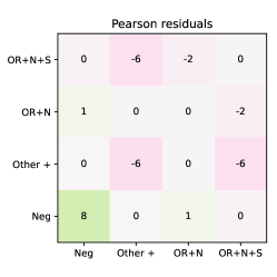
(a) Tranche 1

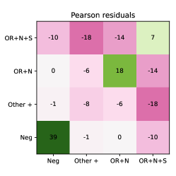
(b) Tranche 2

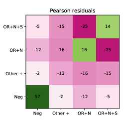
(c) Tranche 3

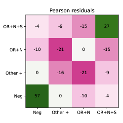
(d) Tranche 4

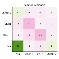
(e) Tranche 5

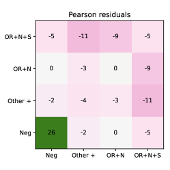
(f) Tranche 6

Figure 5: Residual plots for PCR gene positivity patterns.

to produce the plots in Figure 5.

There are three main patterns of gene positivity that we are interested in: OR+N+S, which is generally seen in common pre-Alpha variants and the Delta variant; OR+N, which is associated with the Alpha variant; or Other, which is usually indicative of too low a viral load to be confident in strain. Where an individual is positive on multiple visits with varying PCR gene positivity patterns, here and throughout we consider the maximal pattern, i.e. that containing the least target failures. So for example, an individual with an N+S positive at one visit followed by an OR+N+S positive at the next visit and then an N positive at the next visit would be counted as an OR+N+S positive overall.

2.5 Full probability model

While the more exploratory methods above are useful for formulating hypotheses, the main part of our analysis will be household regression, using time, household size and individual features to predict positivity. We start by defining a vector and matrix for each household $H_{a},a\in[m]$,

$$\mathbf{y}_{a}:=(y_{i})_{i\in H_{a}}\text{ ,}\qquad\boldsymbol{X}_{a}:=[(\mathbf{x}_{i})_{k}]_{i\in H_{a},k\in[p]}\text{ .}$$ (3)

Note that the outcomes of swab positivity are not independent of each other due to transmission within households, but otherwise the households are selected as uniformly as possible from the population. This means that an independent-households assumption is appropriate, in which we write the likelihood function as

$$L(\boldsymbol{\theta})=\prod_{a\in[m]}P_{\mathbf{y}_{a}}(\boldsymbol{X}_{a},\boldsymbol{\theta})\text{ .}$$ (4)

Here, $\boldsymbol{\theta}$ is a vector of model parameters, and $P_{\mathbf{y}}$ is a function mapping a household feature matrix and set of model parameters onto a probability of a given set of household positivity outcomes. We can derive a set of equations for such probabilities from equation (4) of Addy et al. (1991) as in Kinyanjui and House (2019), and which we present now with some explanation but not a formal derivation of all components.

We will consider the relevant equations for a household $H$ of size $n$ with outcome vector $\mathbf{y}$ and feature matrix $\boldsymbol{X}$ (i.e. suppressing the household index $a$ to simplify notation). In particular, given a map $\iota:\{0,1\}^{n}\rightarrow\{1,\ldots,2^{n}\}$, we will be able to form the vector $\mathbf{P}=(P_{\iota(\mathbf{y})})_{\mathbf{y}\in\{0,1\}^{n}}$ of probabilities of different outcomes in the household. This will be a solution to the set of linear equations

$$\boldsymbol{B}(\boldsymbol{\theta})\mathbf{P}=\mathbf{1}\text{ ,}$$ (5)

where $\mathbf{1}$ is a length-$2^{n}$ vector of all ones, and $\boldsymbol{B}=[B_{\iota(\boldsymbol{\nu}),\iota(\boldsymbol{\omega})}]_{\boldsymbol{\nu},\boldsymbol{\omega}\in\{0,1\}^{n}}$, which has

$$B_{\iota(\boldsymbol{\nu}),\iota(\boldsymbol{\omega})}=\mathcal{B}_{\boldsymbol{\nu},\boldsymbol{\omega}}=\frac{1}{\prod_{j\in H}\Phi\left(\sum_{i\in H}(1-\nu_{i})\lambda_{ij}\right)^{\omega_{j}}Q_{j}^{1-\nu_{j}}}\text{ ,}\quad\boldsymbol{\nu}\leq\boldsymbol{\omega}\in\{0,1\}^{n}\text{ ,}$$ (6)

and other elements equal to zero, where we write $\leq$ between vectors to stand for the statement that each element on the left-hand side is less than or equal to the corresponding element on the right-hand side. The associated condition imposes that each $\boldsymbol{\nu}$ above will correspond to a sub-epidemic of $\boldsymbol{\omega}$ meaning that the equation (5) can be solved iteratively. There are then three main ingredients of the transmission model that we will enumerate below and in doing so define the terms in Equation (6).

The first model component is the probability of avoiding infection from outside; for the $i$-th individual this is

$$Q_{i}=\mathrm{e}^{-\Lambda_{i}}\text{ ,}\qquad\Lambda_{i}=\Lambda\mathrm{e}^{\boldsymbol{\alpha}\cdot\mathbf{x}_{i}}=\mathrm{e}^{\alpha_{0}+\boldsymbol{\alpha}\cdot\mathbf{x}_{i}}\text{ .}$$ (7)

In the language of infectious disease modelling, $\Lambda_{i}$ is the cumulative force of infection experienced by the $i$-th individual. Then $\exp(\alpha_{k})$ is the relative external exposure associated with the $k$-th feature / covariate, meaning that it is the multiplier in front of the baseline force of infection, which is that for an individual whose feature vector is all zeros, $\mathbf{0}$. This baseline probability of avoiding infection from outside is then

$$q=\exp(-\Lambda)=\exp(-\exp(\alpha_{0}))\text{ .}$$ (8)

Because this is often much closer to $1$ than to $0$, we will report the probability of being infected from outside the household as a percentage, i.e. $(1-q)\times 100\%$ will be given in figures and tables. We will present this alongside the relative external exposures that are elements of the vector $\boldsymbol{\alpha}$, although it would also be possible to use (8) to relate $q$ to the baseline force of infection $\Lambda$ or intercept of the linear predictor, $\alpha_{0}$. Note that some care must be taken in interpretation of this variable when the data are split into time periods as in this work, since to appear as a household with at least one positive in one tranche, it is necessary to appear as a household with no positives in the previous tranches for which the household was in the study. Values of $1-q$ will typically be low enough here that this conditional dependence is not strong, but this might not be true at higher levels of incidence for the same design.

The second component of the model is variability in the infectiousness at the individual level, usually interpreted as arising from the distribution of infectious periods. Suppose, in particular, that a household has just one susceptible and one infectious individual, and that the infectious individual exerts a force of infection $\lambda$ on the susceptible for a random period of time $T$. Let the cumulative force of infection be

$$C(t)=\int_{u=0}^{\mathrm{min}(T,t)}\!\!\lambda\,\,\mathrm{d}u\text{ .}$$ (9)

The first step in analysing this model is to apply the Sellke (1983) construction, where the susceptible individual picks a random variable $\Xi\sim\mathrm{Exp}(1)$ and infection happens once $C(t)>\Xi$, or no infection happens if $C(T)<\Xi$. To see why this is equivalent to infection at a rate $\lambda$, take (9) and note that

$$\mathrm{Pr}(\Xi>C(t+\delta t)|\Xi>C(t))=\frac{\int_{0}^{C(t+\delta t)}\mathrm{exp}(-\xi)\mathrm{d}\xi}{\int_{0}^{C(t)}\mathrm{exp}(-\xi)\mathrm{d}\xi}=1-\lambda\delta t+o(\delta t)\text{ .}$$

The furthest right expression in this equation is what we mean by infection at a rate.

Using $F_{X}$ to stand for a cumulative distribution function and $f_{X}$ for a probability density function of a random variable $X$, we have the total probability of avoiding infection as

$$\mathrm{Pr}(\Xi>C(T))=\int_{0}^{\infty}F_{\Xi}(\lambda t)f_{T}(t)\mathrm{d}t=\int_{0}^{\infty}\mathrm{e}^{-\lambda t}f_{T}(t)\mathrm{d}t=\mathcal{L}[f_{T}](\lambda)=:\Phi(\lambda)\text{ ,}$$ (10)

where $\mathcal{L}$ stands for Laplace transformation. We can then use this result to write down the probabilities of different outcomes in a two-person household without covariates:

$$\mathrm{Pr}(\mathbf{y}=(0,0))=Q^{2}\text{ ,}\quad\mathrm{Pr}(\mathbf{y}=(0,1))=\mathrm{Pr}(\mathbf{y}=(1,0))=Q(1-Q)\Phi(\lambda)\text{ ,}$$

which are expressions that can also be obtained from (6). A more general argument is presented by Ball (1986) for the full system of equations, but the expressions above should give some intuition for why these hold.

For our modelling, we assume that each individual picks an infectious period from a unit-mean Gamma distribution since the equations are not sensitive to the mean and this therefore provides a natural one-parameter distribution with appropriate support. The Laplace transform of this as used in (6) is

$$\Phi(s)=(1+\vartheta s)^{-1/\vartheta}\text{ .}$$ (11)

The parameter $\vartheta$ is the variance of the Gamma distribution, i.e. it is larger for more individual variability.

The third component of the model is the infection rate from individual $j$ to individual $i$,

$$\lambda_{ij}=n^{\eta}\lambda\sigma_{i}\tau_{j}=n^{\eta}\lambda\mathrm{e}^{\boldsymbol{\beta}\cdot\mathbf{x}_{i}}\mathrm{e}^{\boldsymbol{\gamma}\cdot\mathbf{x}_{j}}=\mathrm{e}^{\boldsymbol{\beta}\cdot\mathbf{x}_{i}}\mathrm{e}^{\gamma_{0}+\eta\log(n)+\boldsymbol{\gamma}\cdot\mathbf{x}_{j}}\text{ .}$$ (12)

In this equation: $\lambda$ is the baseline rate of infection; $\sigma_{i}=\mathrm{e}^{\boldsymbol{\beta}\cdot\mathbf{x}_{i}}$ is the relative susceptibility of the $i$-th participant, and $\exp(\beta_{k})$ is the relative susceptibility associated with the $k$-th feature; $\tau_{j}=\mathrm{e}^{\boldsymbol{\gamma}\cdot\mathbf{x}_{j}}$ is the relative transmissibility of the $j$-th participant, and $\exp(\gamma_{k})$ is the relative transmissibility associated with the $k$-th feature / covariate. As can be seen from (12), we can interpret $\log(\lambda)$ as the intercept of the linear predictor for transmissibility. The term $n^{\eta}$ is a modelling approach to the effect of household size usually attributed to Cauchemez et al. (2004); as can be seen from (12), this is equivalent to taking $\log(n)$ as a covariate for transmissibility. Experience with fitting these models (Kinyanjui et al., 2018) suggests that it is a good idea to impose hard bounds on the Cauchemez parameter, i.e. insist that $\eta\in[\eta_{\mathrm{min}},\eta_{\mathrm{max}}]$, meaning that here we will treat $\eta$ separately from other parameters.

2.6 Model variables and fitting

We now enumerate all of the model parameters, distinguishing between the ‘natural’ representations of parameters that sit in $\mathbb{R}$ and transforms of natural parameter space $\mathbb{R}^{\kappa}$ that are most epidemiologically interpretable and therefore suitable for reporting. Since $\Lambda$, $\lambda$ and $\vartheta$ have positive support, we can use logarithmic and exponential functions to transform between epidemiological and natural parameters. As noted above, we want $\eta$ to have compact support, and so note that the function $\mathrm{tan}:[-\pi/2,\pi/2]\rightarrow\mathbb{R}$ and its inverse can be used. We choose $\eta_{\mathrm{min}}=-2$ and $\eta_{\mathrm{max}}=2$, meaning that our natural parameter vector is $\boldsymbol{\theta}=(\log(\Lambda),\log(\lambda),\log(\vartheta),\tan(\pi\eta/4),\boldsymbol{\alpha},\boldsymbol{\beta},\boldsymbol{\gamma})\in\mathbb{R}^{\kappa}$.

The first part of this parameter vector is the external force of infection, with natural representation $\alpha_{0}=\log(\Lambda)$. Here we will quote the baseline probability of infection from outside as a percentage, which is $(1-q)\times 100\%$ for $q$ as in (8).

The second part of the parameter space relates to baseline within-household transmission with natural representation $\gamma_{0}=\log(\lambda)$, $\log(\vartheta)$, and $\tan(\pi\eta/4)$, where we use this transform for $\eta$ to make a hard constraint of epidemiologically meaningful values. For interpretability, we work with probabilities of infection by household size, which from generalising (10) to a size-scaled transmission rate are

$$p_{n}=1-\Phi(n^{\eta}\lambda)\text{ .}$$ (13)

Such quantities have been called Susceptible-Infectious Transmission Probabilities (SITP) by e.g. Fraser et al. (2011), who estimated values close to 20% from historical data on the 1918 influenza pandemic.

The third part are features, where we consider:

• Three age groups: 2-11 years old; 12-16 years old; and older.

• Working in a patient-facing role or not.

• Pattern of PCR gene target positivity: OR+N+S, which is associated with pre-Alpha variants and the Delta variant; OR+N, which is associated with the Alpha variant; or other, which is usually indicative of too low a viral load to be confident in strain.

We assume that age and working in a patient-facing role have an association with external risk, leading to natural parameters $\alpha_{\text{2-11}}$, $\alpha_{\text{12-16}}$ and $\alpha_{\text{PF}}$; that age has an association with susceptibility, leading to natural parameters $\beta_{\text{2-11}}$ and $\beta_{\text{12-16}}$; and that age and gene positivity in PCR have an association with transmissibility, leading to natural parameters $\gamma_{\text{2-11}}$, $\gamma_{\text{12-16}}$, $\gamma_{\text{OR+N}}$ and $\gamma_{\text{oth}}$. For any natural parameter $r$, we will report the multiplicative effect $\exp(r)$.

Model fitting was performed in an approximate Bayesian framework using the Laplace approximation. As noted above, households of size 7 and larger were excluded from the analysis partly because these are often very different in composition from smallerhouseholds, and partly because of the numerical cost of solving a linear system of size $2^{n}$ We combine the likelihood (4) with a standard normal prior on natural parameters, $\boldsymbol{\theta}\sim\mathcal{N}_{\kappa}(\mathbf{0},\boldsymbol{I})$. Sensitivity of results to this prior was considered for different variances and revealed essentially no impact on the highly identifiable parameters such as $\Lambda$ and $\lambda$, and that while a higher variance could slightly reduce the shrinkage of effect sizes towards zero, it could also lead to instability in fitting, meaning that this prior achieves regularisation of the inference problem without excessive bias. The maximum a posteriori estimate was obtained using multiple restarts of a Quasi-Newton optimiser. The Hessian was calculated numerically for the natural parameters and used in the Laplace approximation to the posterior on the natural parameters. The credible intervals (CIs) are then transformed from natural to epidemiologically interpretable parameters.

2.7 Data processing and software implementation

The analysis was carried out on the ONS Secure Research Server in the Python 3 language. To illustrate issues with data processing, note that the ‘flat’ form for the data extracted from the database after cleaning takes a form like:

    HID   PID   Visit Date   Age   Test Result   Work PF   Pattern
    ...
    123   456   2020-10-02   8     Negative      No        NA
    123   457   2020-10-02   38    Negative      No        NA
    123   456   2020-10-10   8     Negative      No        NA
    123   457   2020-10-10   38    Positive      No        OR+N+S
    123   456   2020-10-17   9     Positive      No        OR+N+S
    123   457   2020-10-17   38    Negative      No        NA
    ...
    124   458   2021-02-15   53    Negative      Yes       NA
    ...

In particular, there is a hierarchical structure to the data. Households, each with a unique household ID in the HID column, have a number of study participants with a unique participant ID in the PID column, and each participant being visited on a number of dates as in the Visit Date column. Each visit will have associated participant features (e.g. as in the Age column above) and a Test Result.

The large size of this flat file (slightly under three million rows) means that it is advantageous to use specialist libraries, in this case pandas (The pandas development team, 2020; McKinney, 2010) together with NumPy (Harris et al., 2020). To deal with the nested structure of the data, we used the ‘split-apply-combine’ paradigm that this library encourages by analogy with SQL operations. In the example above, this would involve first associating each participant with an age using pandas.groupby(’PID’) and pandas.DataFrame.apply(numpy.min), and then producing an array of ages for each household using pandas.groupby(’HID’) and pandas.DataFrame.apply(numpy.array). A similar approach is possible for test results and multiple features.

Apart from data processing, the main computational cost of the analysis is the linear algebra associated with solving (5), particularly for larger households. Due to portability, this was carried out in NumPy on the ONS system, however we found that implementation in Numba (Lam et al., 2015) can generate significant speed-ups, as might use of GPU hardware through use of e.g. PyTorch (Paszke et al., 2019).

Access to ONS CIS data is possible via the Office for National Statistics’ Secure Research Service, and Python code demonstrating the methodology applied to publicly available data is at https://github.com/thomasallanhouse/covid19-housefs.

3 Results and Discussion

3.1 Exploratory analysis

Figure 2 shows the distribution of positives in households; comparison with Table 2 shows that the numbers of households with two or more positives are much greater than would be expected under the assumption of independence. In fact, some histograms even take a bimodal ‘U’ shape.

This multi-modality is even more apparent in the kernel plots in Figure 3, which also demonstrate that it is common to see households with only child positives, only adult positives, or both. In particular, this suggests that both children and adults can be responsible for bringing infection into the household. While some of the child-infection-only households could arise due to failure of ascertainment of an adult infection in the household, this is unlikely to be true for most, meaning, the introduction of infection to the household would have been due to a child (and vice versa for adult-infection-only households).

3.2 Residual analysis

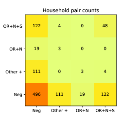
(a) Tranche 1

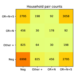
(b) Tranche 2

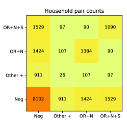
(c) Tranche 3

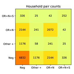
(d) Tranche 4

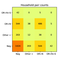
(e) Tranche 5

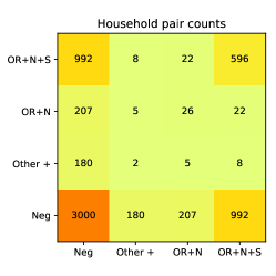
(f) Tranche 6

Figure 4: Pair counts for PCR gene positivity patterns.

The pair counts and Pearson residual analysis – applied to the maximal PCR target gene positivity pattern being OR+N+S, OR+N, other positive, or negative – are shown in Figures 4 and 5. The pair counts show at the household level the replacement of the OR+N+S pattern as the main source of positive pairs in households with the OR+N pattern, and then the return of the OR+N+S pattern. We also see from the residual plots that while there is positive correlation of (OR+N+S)-(OR+N+S) and (OR+N)-(OR+N) pairs, as well as of negative-negative pairs, there is a negative correlation associated with (OR+N+S)-(OR+N) pairs and also between pairs involving any other positive pattern. While this analysis is not mechanistic or causal, we expect that the main factor generating correlation / clustering of positives in households is transmission. As such, the results are consistent with our understanding of the sweeps of the Alpha and Delta variants as arising due to these being more transmissible strains than those that they replaced.

3.3 Regression analysis

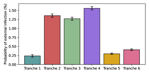
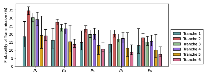
Figure 6: Visualisation of the fitted model. Top: Baseline probability of infection from outside. Bottom: Per-pair baseline probabilities of secondary transmission within the household, not including tertiary transmission effects.

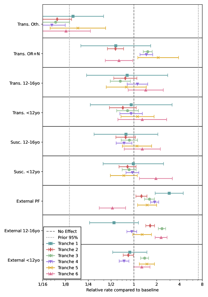
Figure 7: Visualisation of the fitted model. Relative effects on transmission, susceptibility and external exposure compared to baseline of an adult not working in a patient-facing role with OR+N+S maximal PCR gene positivity pattern if positive. ‘Trans.’ stands for relative transmissibility, ‘Susc.’ for relative susceptibility, and ‘External’ for relative external exposure.

The regression analysis has its outputs shown in Table 3, Figure 6, and Figure 7. We now present these in order.

The baseline external probabilities of infection shown in the top plot of Figure 6 follow the rough pattern that would be expected from community prevalence and Tranche duration, with the notable exception of Tranche 6, when it is likely that vaccination significantly reduced the infection risk despite high prevalence. In terms of the baseline probabilities of within-household transmission in the bottom plot of Figure 6, these are largely consistent in terms of overlapping credible intervals for Tranches 2, 3 and 4, with Tranche 6 noticeably lower and with credible intervals that do not overlap with those for Tranches 2, 3 and 4, likely due to the impact of vaccination (and despite the emergence of the Delta variant). The low-prevalence Tranches 1 and 5 have large credible intervals, so are hard to distinguish statistically from the other Tranches, despite having lower point estimates. It is worth noting that for periods of low prevalence following periods of high prevalence, we expect lower viral loads on average as noted by Hay et al. (2021), and this might impact on overall transmissibility estimates.

Turning to Figure 7, we see that ‘other’ patterns of gene positivity (besides OR+N and OR+N+S) are consistently associated with much lower transmissibility, as would be expected given target failure is more likely at lower viral loads(Walker et al., 2021). We also see lower transmissibility of OR+N prior to the emergence of the Alpha variant, since S-gene target failure would have been associated with lower viral loads at that point as well, but higher transmissibility for this pattern after the emergence of Alpha but before the emergence of Delta. After the emergence of Delta, the OR+N pattern is associated with lower transmissibility than OR+N+S, as would be expected.

In terms of child susceptibility and transmissibility, there is no strong evidence for an effect. While it is plausible that non-vaccination of children would lead to increasing their relative susceptibility at later times, this is consistent with the Tranche 6 results but not strongly evidenced by them.

For patient-facing staff, external risk of infection has been consistently high until reduced in Tranche 6, most likely due to the impact of vaccination. For children, external risk of infection is generally raised compared to baseline when schools are open, with the exception of primary school aged children before the emergence of Alpha. Whether this change in association is due to some causal factor not accounted for here, or is related to the new variants spreading more efficiently amongst young children than wildtype, requires further investigation.

3.4 Limitations and directions for future work

While we have taken many steps to ensure that the results presented here are as robust as possible, there are key limitations to the analysis that need to be borne in mind. The main one of these is failures in ascertainment of positives and other missingness in the longitudinal design in question. The most likely consequence of this will be to depress susceptible-infectious transmission probability estimates. One theoretical approach to deal with this would be imputation of the transmission tree as suggested by Demiris and O’Neill (2005), but this is likely to be too computationally intensive to be practical in the current context. Another would be analytical work to include failure of ascertainment into the likelihood function as in House et al. (2012), however it is unclear how to model ascertainment probabilistically in a tractable manner. A data-driven approach would be to try to include positives from other sources such as Test and Trace case data or self-reported episodes of illness. There is also a harder to quantify potential bias of non-participation in the study, particularly if this is with respect to some factor that is not measured.

Another important limitation is the possibility that other features, for example the geographical region that households are in, more detailed information about viral load and symptoms, or information about the physical structure of the household, might play an important explanatory role in the associations observed. Finally, there are possible refinements of the work: trends in external infection over time could be modelled as a flexible functional form (e.g. a spline as in Pouwels et al. (2021)); extra features could be added, and features selected using formal criteria, including relaxing of the Cauchemez assumption to allow transmission probabilities to depend in a general manner on household size, and explicit correction to attack rates due to shrinking and growing epidemics could be made as proposed by Ball and Shaw (Ball and Shaw, 2015; Shaw, 2016); model parameters – e.g. baseline transmission probabilities – could be shared across tranches; the work could be extended to Wales, Scotland and Northern Ireland; more formal analysis of causal pathways could be performed; and improvements could be made in implementation data processing, model evaluation through improved linear algebra, and fitting algorithm. These and other directions should be the subject of future studies.

Tranche	Start date	End date	Prevalence	Schools	Alpha variant	Delta variant	Vaccination
1	26-Apr-20	31-Aug-20	Low	Closed	Not emerged	Not emerged	None
2	1-Sep-20	14-Nov-20	High	Open	Negligible	Not emerged	None
3	15-Nov-20	31-Dec-20	High	Open	Becomes dominant	Not emerged	Negligible
4	1-Jan-21	14-Feb-21	High	Mainly closed	Dominant	Not emerged	$>10$M 1st, negligible 2nd
5	15-Feb-21	29-Apr-21	Low	Open	Dominant	Negligible	$>35$M 1st, $>15$M 2nd
6	30-Apr-21	15-Jul-21	High	Open	Declining	Becomes dominant	$>45$M 1st, $>35$M 2nd

Table 1: Summary of properties of the time periods (tranches) that the data are split into for analysis.

	Tranche 1	Tranche 2	Tranche 3	Tranche 4	Tranche 5	Tranche 6	Overall
Number of participants	89624	293570	315187	329532	343821	351879	408278
Number of households	43300	144904	157432	165238	171809	178955	200876
Number of positive individuals	242	5625	6078	6925	1440	1890	23392
Households with $1+$ positive	206	4074	4433	5123	1071	1506	17180
Children $<$12	7483	23257	24045	24686	25408	25050	32307
Children 12–16	4814	15503	16790	18098	19012	19294	22250
OR+N+S positives	124	4051	2263	695	33	1382	9543
OR+N positives	12	547	2535	4353	1036	244	8842
Patient-facing participants	3335	9464	10046	10069	11103	11437	15213

Table 2: Features of the dataset and different tranches.

	Tranche 1	Tranche 2	Tranche 3	Tranche 4	Tranche 5	Tranche 6
$1-q$	0.237 (0.205,0.274) %	1.35 (1.31,1.4) %	1.27 (1.22,1.31) %	1.56 (1.51,1.61) %	0.296 (0.277,0.317) %	0.408 (0.384,0.433) %
$p_{2}$	18.4 (12.1,27.9) %	34.5 (32.1,37.0) %	30.2 (27.7,33.1) %	29.0 (25.2,33.5) %	19.2 (11.1,31.3) %	18.9 (16.0,22.9) %
$p_{3}$	16.2 (11.3,23.4) %	27.4 (25.7,29.2) %	23.8 (21.8,26.0) %	23.3 (20.1,26.7) %	15.3 (8.92,25.5) %	13.6 (11.8,16.9) %
$p_{4}$	14.8 (10.2,22.0) %	23.0 (21.3,25.2) %	19.8 (17.9,22.5) %	19.7 (16.8,23.6) %	12.9 (7.38,22.6) %	10.7 (9.09,14.6) %
$p_{5}$	13.7 (8.86,22.5) %	20.0 (18.1,22.5) %	17.1 (15.1,20.0) %	17.3 (14.5,21.1) %	11.3 (6.25,20.9) %	8.79 (7.22,13.3) %
$p_{6}$	12.9 (8.06,23.4) %	17.7 (15.7,20.5) %	15.1 (13.0,18.6) %	15.5 (12.7,19.4) %	10.1 (5.4,19.7) %	7.48 (5.97,12.2) %
$\exp(\alpha_{\text{2-11}})$	0.883 (0.525,1.49)	0.845 (0.723,0.987)	1.39 (1.23,1.56)	0.742 (0.64,0.86)	1.48 (1.18,1.87)	1.27 (0.993,1.63)
$\exp(\alpha_{\text{12-16}})$	0.546 (0.26,1.15)	1.64 (1.44,1.87)	2.35 (2.1,2.63)	0.938 (0.807,1.09)	1.29 (0.967,1.71)	2.29 (1.91,2.74)
$\exp(\alpha_{\text{PF}})$	2.93 (1.91,4.49)	1.26 (1.06,1.49)	1.61 (1.38,1.87)	1.88 (1.66,2.13)	1.5 (1.12,2.0)	0.521 (0.349,0.778)
$\exp(\beta_{\text{2-11}})$	0.984 (0.393,2.46)	0.824 (0.636,1.07)	0.865 (0.7,1.07)	0.956 (0.787,1.16)	0.737 (0.49,1.11)	1.95 (1.18,3.22)
$\exp(\beta_{\text{12-16}})$	0.786 (0.298,2.07)	0.778 (0.578,1.05)	0.872 (0.68,1.12)	0.741 (0.583,0.943)	1.1 (0.704,1.71)	1.29 (0.746,2.24)
$\exp(\gamma_{\text{2-11}})$	0.922 (0.266,3.2)	0.715 (0.476,1.07)	0.824 (0.593,1.15)	0.919 (0.652,1.29)	1.12 (0.676,1.85)	1.29 (0.615,2.71)
$\exp(\gamma_{\text{12-16}})$	0.815 (0.237,2.8)	0.771 (0.542,1.1)	0.662 (0.488,0.899)	1.11 (0.815,1.52)	0.794 (0.432,1.46)	1.43 (0.841,2.45)
$\exp(\gamma_{\text{OR+N}})$	0.576 (0.199,1.67)	0.572 (0.447,0.731)	1.52 (1.33,1.75)	1.46 (1.2,1.77)	2.09 (1.13,3.89)	0.636 (0.419,0.965)
$\exp(\gamma_{\text{CT-oth}})$	0.157 (0.062,0.398)	0.097 (0.0626,0.15)	0.0926 (0.0607,0.141)	0.0826 (0.055,0.124)	0.182 (0.0783,0.424)	0.127 (0.0604,0.267)

Table 3: The parameter point estimates and CIs.

Figure 1: Schematic of a hypothetical but realistic data pattern for a four-person household in the first two months after recruitment. Each negative test is shown as a blue circle containing $\times$ and each positive test is shown as a red circle containing $+$. One potential route for infection coming into and transmitting within the household is shown as through a series of red arrows. This is not directly observed in the study design, and in fact other transmission trees (for example one in which PID2 is infected before PID3) are consistent with the data that would be obtained from this household.

(a) Tranche 1

(b) Tranche 2

(c) Tranche 3

References

- Abbey (1952) H. Abbey. An examination of the Reed-Frost theory of epidemics. Human Biology, 24(3):201–233, 1952.
- Addy et al. (1991) C. L. Addy, I. M. Longini, and M. Haber. A generalized stochastic model for the analysis of infectious disease final size data. Biometrics, 47(3):961–974, 1991.
- Bailey (1957) N. T. J. Bailey. The Mathematical Theory of Epidemics. Griffin, London, 1957.
- Ball and Shaw (2015) F. Ball and L. Shaw. Estimating the within-household infection rate in emerging SIR epidemics among a community of households. Journal of Mathematical Biology, 71(6-7):1705–1735, 2015.
- Ball (1986) F. G. Ball. A unified approach to the distribution of total size and total area under the trajectory of infectives in epidemics models. Advances in Applied Probability, 18(2):289–310, 1986.
- Bhattacharya et al. (2021) A. Bhattacharya, S. M. Collin, J. Stimson, S. Thelwall, O. Nsonwu, S. Gerver, J. Robotham, M. Wilcox, S. Hopkins, and R. Hope. Healthcare-associated COVID-19 in England: a national data linkage study. medRxiv, 2021. DOI: 10.1101/2021.02.16.21251625.
- Bishop et al. (1975) Y. Bishop, S. E. Fienberg, and P. W. Holland. Discrete Multivariate Analysis: Theory and Practice. Massachusetts Institute of Technology Press, Cambridge, 1975.
- Cauchemez et al. (2004) S. Cauchemez, F. Carrat, C. Viboud, A. J. Valleron, and P. Y. Boëlle. A Bayesian MCMC approach to study transmission of influenza: application to household longitudinal data. Statistics in Medicine, 23(22):3469–3487, 2004.
- Challen et al. (2021) R. Challen, E. Brooks-Pollock, J. M. Read, L. Dyson, K. Tsaneva-Atanasova, and L. Danon. Risk of mortality in patients infected with SARS-CoV-2 variant of concern 202012/1: matched cohort study. BMJ, 372:n579, 2021.
- Dattner et al. (2021) I. Dattner, Y. Goldberg, G. Katriel, R. Yaari, N. Gal, Y. Miron, A. Ziv, R. Sheffer, Y. Hamo, and A. Huppert. The role of children in the spread of COVID-19: Using household data from Bnei Brak, Israel, to estimate the relative susceptibility and infectivity of children. PLOS Computational Biology, 17(2):1–19, 2021.
- Davies et al. (2020) N. G. Davies, P. Klepac, Y. Liu, K. Prem, M. Jit, C. A. B. Pearson, B. J. Quilty, A. J. Kucharski, H. Gibbs, S. Clifford, A. Gimma, K. van Zandvoort, J. D. Munday, C. Diamond, W. J. Edmunds, R. M. G. J. Houben, J. Hellewell, T. W. Russell, S. Abbott, S. Funk, N. I. Bosse, Y. F. Sun, S. Flasche, A. Rosello, C. I. Jarvis, R. M. Eggo, and CMMID COVID-19 working group. Age-dependent effects in the transmission and control of COVID-19 epidemics. Nature Medicine, 26(8):1205–1211, 2020.
- Davies et al. (2021) N. G. Davies, S. Abbott, R. C. Barnard, C. I. Jarvis, A. J. Kucharski, J. D. Munday, C. A. B. Pearson, T. W. Russell, D. C. Tully, A. D. Washburne, T. Wenseleers, A. Gimma, W. Waites, K. L. M. Wong, K. van Zandvoort, J. D. Silverman, CMMID COVID-19 working group, K. COVID-19 Genomics UK (COG-UK) Consortium Diaz-Ordaz, R. Keogh, R. M. Eggo, S. Funk, M. Jit, K. E. Atkins, and W. J. Edmunds. Estimated transmissibility and impact of SARS-CoV-2 lineage B.1.1.7 in England. Science, page eabg3055, 2021. DOI: 10.1126/science.abg3055.
- Demiris and O’Neill (2005) N. Demiris and P. D. O’Neill. Bayesian inference for stochastic multitype epidemics in structured populations via random graphs. Journal of the Royal Statistical Society: Series B (Statistical Methodology), 67(5):731–745, 2005.
- Endo et al. (2019) A. Endo, M. Uchida, A. J. Kucharski, and S. Funk. Fine-scale family structure shapes influenza transmission risk in households: Insights from primary schools in Matsumoto city, 2014/15. PLOS Computational Biology, 15(12):e1007589, 2019.
- Frampton et al. (2021) D. Frampton, T. Rampling, A. Cross, H. Bailey, J. Heaney, M. Byott, R. Scott, R. Sconza, J. Price, M. Margaritis, M. Bergstrom, M. J. Spyer, P. B. Miralhes, P. Grant, S. Kirk, C. Valerio, Z. Mangera, T. Prabhahar, J. Moreno-Cuesta, N. Arulkumaran, M. Singer, G. Y. Shin, E. Sanchez, S. M. Paraskevopoulou, D. Pillay, R. A. McKendry, M. Mirfenderesky, C. F. Houlihan, and E. Nastouli. Genomic characteristics and clinical effect of the emergent SARS-CoV-2 B.1.1.7 lineage in London, UK: a whole-genome sequencing and hospital-based cohort study. The Lancet Infectious Diseases, 21(9):1246–1256, 2021.
- Fraser et al. (2011) C. Fraser, D. A. T. Cummings, D. Klinkenberg, D. S. Burke, and N. M. Ferguson. Influenza transmission in households during the 1918 pandemic. American Journal of Epidemiology, 174(5):505–514, 2011.
- Frost (1976) W. H. Frost. Some conceptions of epidemics in general. American Journal of Epidemiology, 103(2):141–151, 1976.
- Grint et al. (2021) D. J. Grint, K. Wing, E. Williamson, H. I. McDonald, K. Bhaskaran, D. Evans, S. J. Evans, A. J. Walker, G. Hickman, E. Nightingale, A. Schultze, C. T. Rentsch, C. Bates, J. Cockburn, H. J. Curtis, C. E. Morton, S. Bacon, S. Davy, A. Y. Wong, A. Mehrkar, L. Tomlinson, I. J. Douglas, R. Mathur, P. Blomquist, B. MacKenna, P. Ingelsby, R. Croker, J. Parry, F. Hester, S. Harper, N. J. DeVito, W. Hulme, J. Tazare, B. Goldacre, L. Smeeth, and R. M. Eggo. Case fatality risk of the SARS-CoV-2 variant of concern B.1.1.7 in England, 16 November to 5 February. Eurosurveillance, 26(11):2100256, 2021.
- Harris et al. (2020) C. R. Harris, K. J. Millman, S. J. van der Walt, R. Gommers, P. Virtanen, D. Cournapeau, E. Wieser, J. Taylor, S. Berg, N. J. Smith, R. Kern, M. Picus, S. Hoyer, M. H. van Kerkwijk, M. Brett, A. Haldane, J. F. del Río, M. Wiebe, P. Peterson, P. Gérard-Marchant, K. Sheppard, T. Reddy, W. Weckesser, H. Abbasi, C. Gohlke, and T. E. Oliphant. Array programming with NumPy. Nature, 585(7825):357–362, 2020.
- Hay et al. (2021) J. A. Hay, L. Kennedy-Shaffer, S. Kanjilal, N. J. Lennon, S. B. Gabriel, M. Lipsitch, and M. J. Mina. Estimating epidemiologic dynamics from cross-sectional viral load distributions. Science, 373(6552):eabh0635, 2021.
- Hope Simpson (1952) R. E. Hope Simpson. Infectiousness of communicable diseases in the household: (measles, chickenpox, and mumps). The Lancet, 260(6734):549–554, 1952. Originally published as Volume 2, Issue 6734.
- House et al. (2012) T. House, N. Inglis, J. V. Ross, F. Wilson, S. Suleman, O. Edeghere, G. Smith, B. Olowokure, and M. J. Keeling. Estimation of outbreak severity and transmissibility: Influenza A(H1N1)pdm09 in households. BMC Medicine, 10(117):https://doi.org/10.1186/1741–7015–10–117, 2012.
- Kinyanjui and House (2019) T. Kinyanjui and T. House. Generalised linear models for dependent binary outcomes with applications to household stratified pandemic influenza data, 2019. [arXiv:1911.12115].
- Kinyanjui et al. (2018) T. Kinyanjui, J. Middleton, S. Güttel, J. Cassell, J. Ross, and T. House. Scabies in residential care homes: Modelling, inference and interventions for well-connected population sub-units. PLOS Computational Biology, 14(3):e1006046, 2018.
- Kombe et al. (2019) I. K. Kombe, P. K. Munywoki, M. Baguelin, D. J. Nokes, and G. F. Medley. Model-based estimates of transmission of respiratory syncytial virus within households. Epidemics, 27:1–11, 2019.
- Lam et al. (2015) S. K. Lam, A. Pitrou, and S. Seibert. Numba: A LLVM-based Python JIT compiler. In Proceedings of the Second Workshop on the LLVM Compiler Infrastructure in HPC, number 7 in LLVM ’15, 2015. DOI: 10.1145/2833157.2833162.
- Li et al. (2021) F. Li, Y.-Y. Li, M.-J. Liu, L.-Q. Fang, N. E. Dean, G. W. K. Wong, X.-B. Yang, I. Longini, M. E. Halloran, H.-J. Wang, P.-L. Liu, Y.-H. Pang, Y.-Q. Yan, S. Liu, W. Xia, X.-X. Lu, Q. Liu, Y. Yang, and S.-Q. Xu. Household transmission of SARS-CoV-2 and risk factors for susceptibility and infectivity in Wuhan: A retrospective observational study. The Lancet Infectious Diseases, 2021. https://doi.org/10.1016/S1473-3099(20)30981-6.
- Madewell et al. (2020) Z. J. Madewell, Y. Yang, J. Longini, Ira M., M. E. Halloran, and N. E. Dean. Household transmission of SARS-CoV-2: A systematic review and meta-analysis. JAMA Network Open, 3(12):e2031756, 2020.
- McKinney (2010) W. McKinney. Data Structures for Statistical Computing in Python. In Stéfan van der Walt and Jarrod Millman, editors, Proceedings of the 9th Python in Science Conference, pages 56–61, 2010. DOI: 10.25080/Majora-92bf1922-00a.
- Neal (2012) P. Neal. Efficient likelihood-free Bayesian computation for household epidemics. Statistics and Computing, 22(6):1239–1256, 2012.
- Office for National Statistics (2019) Office for National Statistics. Families and households, Edition: 15 November, 2019. https://www.ons.gov.uk/peoplepopulationandcommunity/birthsdeathsandmarriages/families/ datasets/familiesandhouseholdsfamiliesandhouseholds.
- Office for National Statistics (2021) Office for National Statistics. Coronavirus (COVID-19) latest insights: Vaccines, 2021. URL https://www.ons.gov.uk/peoplepopulationandcommunity/healthandsocialcare/conditionsanddiseases/articles/coronaviruscovid19latestinsights/vaccines.
- O’Neill and Roberts (1999) P. D. O’Neill and G. O. Roberts. Bayesian inference for partially observed stochastic epidemics. Journal of the Royal Statistical Society: Series A (Statistics in Society), 162(1):121–129, 1999.
- Paszke et al. (2019) A. Paszke, S. Gross, F. Massa, A. Lerer, J. Bradbury, G. Chanan, T. Killeen, Z. Lin, N. Gimelshein, L. Antiga, A. Desmaison, A. Kopf, E. Yang, Z. DeVito, M. Raison, A. Tejani, S. Chilamkurthy, B. Steiner, L. Fang, J. Bai, and S. Chintala. PyTorch: An imperative style, high-performance deep learning library. In H. Wallach, H. Larochelle, A. Beygelzimer, F. d’Alché Buc, E. Fox, and R. Garnett, editors, Advances in Neural Information Processing Systems 32, pages 8024–8035. Curran Associates, Inc., 2019. http://papers.neurips.cc/paper/9015-pytorch-an-imperative-style-high-performance-deep-learning-library.pdf.
- Pouwels et al. (2021) K. B. Pouwels, T. House, E. Pritchard, J. V. Robotham, P. J. Birrell, A. Gelman, K.-D. Vihta, N. Bowers, I. Boreham, H. Thomas, J. Lewis, I. Bell, J. I. Bell, J. N. Newton, J. Farrar, I. Diamond, P. Benton, A. S. Walker, D. Crook, P. C. Matthews, T. Peto, N. Stoesser, A. Howarth, G. Doherty, J. Kavanagh, K. K. Chau, S. B. Hatch, D. Ebner, L. Martins Ferreira, T. Christott, B. D. Marsden, W. Dejnirattisai, J. Mongkolsapaya, S. Hoosdally, R. Cornall, D. I. Stuart, G. Screaton, D. Eyre, J. Bell, S. Cox, K. Paddon, T. James, J. N. Newton, J. V. Robotham, P. Birrell, H. Jordan, T. Sheppard, G. Athey, D. Moody, L. Curry, P. Brereton, J. Hay, H. Vansteenhouse, A. Lambert, E. Rourke, S. Hawkes, S. Henry, J. Scruton, P. Stokes, T. Thomas, J. Allen, R. Black, H. Bovill, D. Braunholtz, D. Brown, S. Collyer, M. Crees, C. Daglish, B. Davies, H. Donnarumma, J. Douglas-Mann, A. Felton, H. Finselbach, E. Fordham, A. Ipser, J. Jenkins, J. Jones, K. Kent, G. Kerai, L. Lloyd, V. Masding, E. Osborn, A. Patel, E. Pereira, T. Pett, M. Randall, D. Reeve, P. Shah, R. Snook, R. Studley, E. Sutherland, E. Swinn, A. Tudor, J. Weston, S. Leib, J. Tierney, G. Farkas, R. Cobb, F. Van Galen, L. Compton, J. Irving, J. Clarke, R. Mullis, L. Ireland, D. Airimitoaie, C. Nash, D. Cox, S. Fisher, Z. Moore, J. McLean, and M. Kerby. Community prevalence of SARS-CoV-2 in England from April to November, 2020: results from the ONS Coronavirus Infection Survey. The Lancet Public Health, 6(1):e30–e38, 2021.
- Public Health England (2021a) Public Health England. Vaccinations in United Kingdom, 2021a. URL https://coronavirus.data.gov.uk/details/vaccinations.
- Public Health England (2021b) Public Health England. SARS-CoV-2 variants of concern and variants under investigation in England: technical briefing 10, 2021b. URL https://assets.publishing.service.gov.uk/government/uploads/system/uploads/attachment_data/file/984274/Variants_of_Concern_VOC_Technical_Briefing_10_England.pdf.
- Public Health England (2021c) Public Health England. Investigation of novel SARS-CoV-2 variant 202012/01: technical briefing 1, 2021c. URL https://assets.publishing.service.gov.uk/government/uploads/system/uploads/attachment_data/file/959438/Technical_Briefing_VOC_SH_NJL2_SH2.pdf.
- Rambaut et al. (2020a) A. Rambaut, E. C. Holmes, Á. O’Toole, V. Hill, J. T. McCrone, C. Ruis, L. du Plessis, and O. G. Pybus. A dynamic nomenclature proposal for SARS-CoV-2 lineages to assist genomic epidemiology. Nature Microbiology, 5(11):1403–1407, 2020a.
- Rambaut et al. (2020b) A. Rambaut, N. Loman, O. Pybus, W. Barclay, J. Barrett, A. Carabelli, T. Connor, T. Peacock, D. L. Robertson, E. Volz, and COVID-19 Genomics Consortium UK (CoG-UK). Preliminary genomic characterisation of an emergent SARS-CoV-2 lineage in the UK defined by a novel set of spike mutations, 2020b. https://virological.org/t/preliminary-genomic-characterisation-of-an-emergent-sars-cov-2-lineage-in-the-uk-defined-by-a-novel-set-of-spike-mutations/563.
- Reukers et al. (2021) D. F. M. Reukers, M. van Boven, A. Meijer, N. Rots, C. Reusken, I. Roof, A. B. van Gageldonk-Lafeber, W. van der Hoek, and S. van den Hof. High infection secondary attack rates of SARS-CoV-2 in Dutch households revealed by dense sampling. Clinical Infectious Diseases, page ciab237, 2021.
- Scientific Advisory Group for Emergencies (2021) Scientific Advisory Group for Emergencies. Reducing within- and between-household transmission in light of new variant SARS-CoV-2, 14 January, 2021. Paper prepared by the Environmental Modelling Group (EMG), the Scientific Pandemic Insights Group on Behaviours (SPI-B) and the Scientific Pandemic Influenza Group on Modelling (SPI-M).
- Sellke (1983) T. Sellke. On the asymptotic distribution of the size of a stochastic epidemic. Journal of Applied Probability, 20:390–394, 1983.
- Shaw (2016) L. Shaw. SIR epidemics in a population of households. PhD thesis, The University of Nottingham, 2016. http://eprints.nottingham.ac.uk/38606/1/LaurenceShawThesis4185911.pdf.
- The pandas development team (2020) The pandas development team. Pandas, 2020. https://doi.org/10.5281/zenodo.3509134.
- van Boven et al. (2010) M. van Boven, T. Donker, M. van der Lubben, R. B. van Gageldonk-Lafeber, D. E. te Beest, M. Koopmans, A. Meijer, A. Timen, C. Swaan, A. Dalhuijsen, S. Hahné, A. van den Hoek, P. Teunis, M. A. B. van der Sande, and J. Wallinga. Transmission of novel influenza A(H1N1) in households with post-exposure antiviral prophylaxis. PLOS ONE, 5(7):e11442, 2010.
- Walker et al. (2021) A. S. Walker, E. Pritchard, T. House, J. V. Robotham, P. J. Birrell, I. Bell, J. I. Bell, J. N. Newton, J. Farrar, I. Diamond, R. Studley, J. Hay, K.-D. Vihta, T. E. A. Peto, N. Stoesser, P. C. Matthews, D. W. Eyre, K. Pouwels, and the COVID-19 Infection Survey team. Ct threshold values, a proxy for viral load in community SARS-CoV-2 cases, demonstrate wide variation across populations and over time. medRxiv, 2021. DOI: 10.1101/2020.10.25.20219048.
- World Health Organization (2020) World Health Organization. WHO Director-General’s opening remarks at the media briefing on COVID-19-11 March 2020, 2020.
- World Health Organization (2021) World Health Organization. Tracking SARS-CoV-2 variants, 2021. URL https://www.who.int/en/activities/tracking-SARS-CoV-2-variants/.