Scale-Invariant Quadratic Gravity and Inflation in the Palatini Formalism

Abstract

In the framework of classical scale invariance, we consider quadratic gravity in the Palatini formalism and investigate the inflationary predictions of the theory. Our model corresponds to a two-field scalar-tensor theory, that involves the Higgs field and an extra scalar field stemming from a gauge $U(1)_{X}$ extension of the Standard Model, which contains an extra gauge boson and three right-handed neutrinos. Both scalar fields couple nonminimally to gravity and induce the Planck scale dynamically, once they develop vacuum expectation values. By means of the Gildener-Weinberg approach, we describe the inflationary dynamics in terms of a single scalar degree of freedom along the flat direction of the tree-level potential. The one-loop effective potential in the Einstein frame exhibits plateaus on both sides of the minimum and thus the model can accommodate both small and large field inflation. The inflationary predictions of the model are found to comply with the latest bounds set by the Planck collaboration for a wide range of parameters and the effect of the quadratic in curvature terms is to reduce the value of the tensor-to-scalar ratio.

1 Introduction

The combined analysis of the latest cosmological data based on various observations such as the cosmic microwave background (CMB), the large scale structures, the supernova data etc., favor [1] a flat, homogeneous and isotropic Universe. Cosmic inflation [2, 3, 4, 5] not only naturally explains the aforementioned features of the Universe, but quite importantly, when treated quantum mechanically, it also provides a mechanism for the production of the necessary primordial anisotropies, which act as seeds for the generation of the large scale structures that we observe today. Data from the Planck mission combined with previous observations [6] have severely constrained the parameter space of the inflationary models and essentially ruled out many of those, including the simplest ones where a scalar field is minimally coupled to gravity. On the other hand, more involved models such as the Starobinsky [2], where an $\mathcal{R}^{2}$ term is added to the Einstein-Hilbert action, seem to lie within the allowed range. This kind of nonminimal models belongs in the general class of scalar-tensor (ST) theories [7, 8, 9, 10, 11, 12, 13, 14, 15, 16, 17, 18, 19, 20, 21, 22]. In such models, the scalar field $\phi$ typically couples to gravity via a term of the form $\xi\phi^{2}\mathcal{R}$, where $\xi$ is a dimensionless coupling constant and $\mathcal{R}$ is the Ricci scalar. It is noteworthy that this type of coupling allows for the Planck scale to be generated dynamically when $\phi$ develops a vacuum expectation value (VEV).

The dynamical generation of the Planck scale is usually achieved in scale-invariant theories [23, 24, 25, 26, 27, 28, 29, 30, 31, 32, 33, 34, 35, 36, 37, 38, 39, 40, 41, 42, 43, 44, 45, 46, 47, 48, 49, 50, 51, 52, 53, 54, 55, 56, 57, 58, 59, 60, 61, 62, 63, 64, 65, 66, 67, 68, 69, 70], where the running of the inflaton quartic coupling induces symmetry breaking à la Coleman–Weinberg. Scale invariance posits that the Lagrangian of a theory should not contain any ad hoc mass parameters. Utilizing the restrictive power of scale invariance, one can built three more terms that respect the symmetry: the Starobinsky term $\alpha\mathcal{R}^{2}$ and the terms $\beta\mathcal{R}_{\mu\nu}\mathcal{R}^{\mu\nu}$ and $\gamma\mathcal{R}_{\mu\nu\sigma\lambda}\mathcal{R}^{\mu\nu\sigma\lambda}$, where $\mathcal{R}_{\mu\nu\sigma\lambda}$ and $\mathcal{R}_{\mu\nu}$ are the Riemann and Ricci tensors, respectively, and $\alpha$, $\beta$ and $\gamma$ are dimensionless constants. This gravitational theory is called quadratic gravity and has recently received a lot of attention as a possible realization of quantum gravity [71, 72, 73, 74, 35, 75, 47, 76, 77, 63, 78, 62, 79, 80, 70, 81]. Of course, in extended theories of gravity, the issue of the correct formulation arises, i.e. whether one should employ the metric or the Palatini formalism when varying the action.

It has been known that the Palatini formulation [82, 83] of General Relativity (GR) (first-order formalism) is an alternative to the well-known metric formulation (second-order formalism). In the latter, the spacetime connection is the usual Levi-Civita one, while in the Palatini approach the connection $\Gamma^{\lambda}_{\,\,\mu\nu}$ and the metric $g_{\mu\nu}$ are treated as independent variables. In the context of GR, the two formalisms are equivalent at the level of the field equations, with the Levi-Civita connection in the Palatini approach being recovered on shell. When nonminimal couplings between gravity and matter [84, 85, 86, 87, 88, 89, 90, 91, 92, 93, 94, 95, 96, 97, 98, 99, 100, 101, 102, 103, 104, 105, 106, 65, 107, 108, 109, 20, 110, 111, 112, 113, 114, 21, 115, 116, 117, 118, 22, 119, 120, 121] or/and $f(R)$ theories [122, 123, 124, 125, 126, 127, 128, 129, 130, 131, 132, 133, 134, 80, 135, 69, 70, 136, 137, 138, 139, 140] are considered, the resultant field equations are no longer the same and thus the two formalisms lead to different cosmological predictions. A remarkable example is the Starobinsky model of inflation [2], where the addition of an $\mathcal{R}^{2}$ term in the usual Einstein-Hilbert action is translated to a new propagating scalar degree of freedom which plays the role of the inflaton. In the Palatini formalism there are no extra propagating degrees of freedom, therefore the inflaton has to be added ad hoc in the action. The advantage of considering the Palatini formulation is that the addition of the $R^{2}$ term can be used to reduce the tensor-to-scalar ratio $r$ [124]. Thereby, various models where inflation is driven by a scalar field can be rendered again compatible with the observations [125, 126]. Furthermore, the addition of a symmetric Ricci tensor squared term $R_{(\mu\nu)}R^{(\mu\nu)}$ in the Einstein-Hilbert action has the same effect as the pure $R^{2}$ term (see [141]), at least with respect to the modification of the scalar potential, and consequently leads to the reduction of the tensor-to-scalar ratio [124]. The main, but not significant, difference between these two quadratic scale-invariant terms is that in the Einstein frame (EF) the $R^{2}$ term translates also to a second-order kinetic term, while the $R_{(\mu\nu)}R^{(\mu\nu)}$ term yields a series of higher-order kinetic terms. These higher-order kinetic terms are nevertheless negligible at least during slow roll.

In this paper we construct a model of scale-invariant quadratic gravity, where the Planck scale is dynamically generated through the VEVs of a scalar field $\phi$ and the Higgs $h$, which are nonminimally coupled to gravity through terms of the form $\xi_{i}\Phi_{i}^{2}R$, where $\Phi_{i}=\phi,\,h$. The extra scalar field $\phi$ stems from a general $U(1)_{X}$ extension of the Standard Model (SM) gauge structure that contains an extra gauge boson $X_{\mu}$ and three right-handed neutrinos $N_{R}$ that can generate masses for the SM neutrinos via a type-I seesaw mechanism. The model can easily accommodate dark matter in a natural way and we outline three distinct possibilities. Moreover, the mass of the Higgs and the electroweak scale is generated through a portal coupling between $\phi$ and $h$ of the form $\lambda_{h\phi}h^{2}\phi^{2}$. Thus, the addition of the extra scalar field $\phi$ is necessary to preserve the scale invariance of our model since the known Higgs mass term contained in the SM Lagrangian is not scale invariant.

The rest of the paper is organised as follows: In Section 2, we describe the beyond SM (BSM) part of the model, along with the extended gravity part that contains terms quadratic in curvature and is studied in the Palatini formulation. We also briefly describe the dark matter candidates that can arise from our setup. Then, in Section 3, we employ the Gildener-Weinberg approach [142] (which is a generalization of the Coleman-Weinberg mechanism [143] to multiple fields) in order to obtain the flat direction of the tree-level potential. Along the flat direction, the theory effectively becomes single field and by computing the quantum corrections we obtain the one-loop effective potential, which is stable due to the extra $U(1)_{X}$ gauge boson. In Section 4, we introduce an auxiliary field $\Sigma_{\mu\nu}$ in order to parametrize the terms quadratic in curvature. By applying a Weyl rescaling and a disformal transformation of the metric, we obtain the EF representation of the theory. In the process, higher-order kinetic terms arise, but these have been shown to not significantly influence the inflationary [132] and reheating [139] dynamics. At the same time, the EF potential is modified and develops plateaus on both sides of the VEV. In Section 5, we obtain the inflationary predictions of the model in the slow roll approximation and impose constraints on the free parameters. Finally, we summarize and conclude in Section 6. Further details about the disformal transformation are relegated to the Appendices.

We use natural units $\hbar=c=k_{\mathrm{B}}=1$ and the metric signature $(-,\!+,\!+,\!+)$ throughout. We also use $M_{\rm P}^{2}=1$ in most formulas except when we want the dimensionality to be explicit.

2 The model

We begin the discussion of our model by describing the scale-invariant $U(1)_{X}$ extension of the SM that we use [144, 145, 146, 147, 148, 149, 150, 151, 152, 153, 154, 155, 156, 157, 158, 159, 160, 161, 162], which contains a complex scalar field $\Phi$, a gauge boson $X_{\mu}$ and three right-handed neutrinos $N^{i}_{R}$. We also outline three distinct possibilities for the model to accommodate dark matter candidates. Subsequently, we focus on the gravity part of the theory and study it in the Palatini formalism.

2.1 $U(1)_{X}$ extension of the Standard Model

We consider the $U(1)_{X}$ extension of the SM based on the gauge group $SU(3)_{c}\crossproduct SU(2)_{L}\crossproduct U(1)_{Y}\crossproduct U(1)_{X}$. In Table 1 we present the matter fields of this model which contains the SM matter fields along with three generations of right-handed neutrinos $N^{i}_{R}$ ($i=1,2,3$) and a $U(1)_{X}$ complex scalar field $\Phi$, whose VEV will generate the mass of the vector boson $X_{\mu}$ as well as the masses of the right-handed neutrinos. This $U(1)_{X}$ extension can be recognized as a linear combination of the $U(1)_{Y}$ and the $U(1)_{B-L}$ gauge group, with the latter being free of gauge and gravitational anomalies. The existence of the three right-handed neutrinos plays a crucial role to this anomaly cancellation. Following [163] we introduce the real parameters $x_{H}$ and $x_{\Phi}$ which are used in the determination of the $U(1)_{X}$ charge of the field $\Phi$, that is given by

$$Q_{X}=Yx_{H}+Q_{BL}\;x_{\Phi}\,,$$ (2.1)

with $Y$ and $Q_{BL}$ being its hypercharge and $B-L$ charge respectively. Two interesting choices for the parameters $x_{H}$ and $x_{\Phi}$ are the choice $(x_{H},x_{\Phi})=(0,1)$, which corresponds to the $U(1)_{B-L}$ model and the $(x_{H},x_{\Phi})=(-2,1)$ choice which coincides with the SM with an additional $U(1)_{R}$ symmetry.

The covariant derivative associated with the $U(1)_{Y}\crossproduct U(1)_{X}$ gauge interaction is defined as

$$D_{\mu}=\partial_{\mu}-i\left(g_{1}Y+\tilde{g}Q_{X}\right)B_{\mu}-ig_{X}Q_{X}X_{\mu}\,,$$ (2.2)

where $g_{1}$ and $g_{X}$ are the $U(1)_{Y}$ and $U(1)_{X}$ gauge couplings respectively. In (2.2), the possible kinetic mixing between the two $U(1)$ gauge bosons can be ignored for simplicity assuming that the mixing coupling $\tilde{g}$ vanishes at the $U(1)_{X}$ symmetry breaking scale.

	$SU(3)_{c}$	$SU(2)_{L}$	$U(1)_{Y}$	$U(1)_{X}$
$q^{i}_{L}$	3	2	$1/6$	$(1/6)x_{H}+(1/3)x_{\Phi}$
$u^{i}_{R}$	3	1	$2/3$	$(2/3)x_{H}+(1/3)x_{\Phi}$
$d^{i}_{R}$	3	1	$-1/3$	$(-1/3)x_{H}+(1/3)x_{\Phi}$
$\ell^{i}_{L}$	1	2	$-1/2$	$(-1/2)x_{H}+(-1)x_{\Phi}$
$e^{i}_{R}$	1	1	$-1$	$(-1)x_{H}+(-1)x_{\Phi}$
$H$	1	2	$1/2$	$(1/2)x_{H}$
$N^{i}_{R}$	1	1	$0$	$(-1)x_{\Phi}$
$\Phi$	1	1	$0$	$(+2)x_{\Phi}$

Table 1: The matter fields of the $U(1)_{X}$ extension of the SM along with the corresponding charges. In addition to the SM particle content ($i=1,2,3$), three right-handed neutrinos $N_{R}^{i}$ ($i=1,2,3$) and a $U(1)_{X}$ complex scalar field $\Phi$ are introduced. The $U(1)_{X}$ charge is determined by the two real parameters, $x_{H}$ and $x_{\Phi}$, as $Q_{X}=Yx_{H}+Q_{BL}\,x_{\Phi}$ with its hypercharge $Y$ and $B-L$ charge $Q_{BL}$.

In the known SM Yukawa sector we need to add the BSM Yukawa sector arising from the $U(1)_{X}$ extension which reads

$$\mathcal{L}^{\rm BSM}_{\rm Yukawa}=-y_{D}^{ij}\overline{\ell}^{i}_{L}HN^{j}_{R}-\frac{1}{2}y_{M}^{i}\Phi\overline{N}^{iC}_{R}N^{i}_{R}+h.c.\,,$$ (2.3)

where $y_{D}$ and $y_{M}$ are the Dirac and Majorana Yukawa couplings respectively. Also, without loss of generality, the Majorana Yukawa couplings are assumed to be already diagonal in our basis. Furthermore, it is interesting to note that in this setting a lepton asymmetry can be generated from decays of the heavy right-handed neutrinos into SM leptons at high temperatures. Then, the lepton asymmetry can be converted into a baryon asymmetry via electroweak sphalerons [164, 165] (see also [151, 166, 167]).

Assuming that the $U(1)_{X}$ complex scalar field $\Phi$ develops a nonzero VEV $v_{\phi}$ and working in the unitary gauge, we have that

$$\Phi=\frac{1}{\sqrt{2}}(\phi+v_{\phi})\,.$$ (2.4)

Thus, the BSM scalar Lagrangian and the gravity Lagrangian are given by

$$\mathcal{L}^{\rm BSM}_{\rm scalar} = -\frac{1}{2}g^{\mu\nu}\partial_{\mu}\phi\partial_{\nu}\phi-\frac{1}{4}\lambda_{\phi}\phi^{4}+\frac{1}{4}\lambda_{h\phi}h^{2}\phi^{2}\,,$$

$$\mathcal{L}_{\rm gravity} = \frac{1}{2}\left(\xi_{\phi}\phi^{2}+\xi_{h}h^{2}\right)g^{\mu\nu}R_{\mu\nu}(\Gamma)\,,$$ (2.5)

where $h$ is the Higgs field also written in the unitary gauge and $\xi_{\phi}$, $\xi_{h}$ are the nonminimal couplings between gravity and matter. Note that the Ricci tensor depends only on the connection $\Gamma$ since we are working in the Palatini formalism. Also, there are no mass terms for either $\phi$ or $h$ since the theory must respect classical scale invariance. The reduced Planck mass $M_{\rm P}$ is generated dynamically when $\phi$ and h develop their VEVs,

$$M^{2}_{\rm P}=\xi_{\phi}v_{\phi}^{2}+\xi_{h}v_{h}^{2}\,.$$ (2.6)

Associated with the $U(1)_{X}$ and the electroweak symmetry breaking, the $U(1)_{X}$ gauge boson $X_{\mu}$ and the Majorana right-handed neutrinos $N^{i}_{R}$ acquire their masses as

$$M_{X}=\sqrt{\left(2x_{\Phi}g_{X}v_{\phi}\right)^{2}+\left(x_{H}g_{X}v_{h}\right)^{2}}\simeq 2x_{\Phi}g_{X}v_{\phi}\,,\qquad M_{N^{i}_{R}}=\frac{y^{i}_{M}}{\sqrt{2}}v_{\phi}\,.$$ (2.7)

The part of the action that contains the scalar $\phi$ and the Higgs $h$ is

$$S=\int\differential^{4}x\sqrt{-g}\left[\frac{1}{2}\left(\xi_{\phi}\phi^{2}+\xi_{h}h^{2}\right)g^{\mu\nu}R_{\mu\nu}(\Gamma)-\frac{1}{2}g^{\mu\nu}\partial_{\mu}\phi\partial_{\nu}\phi-\frac{1}{2}g^{\mu\nu}\partial_{\mu}h\partial_{\nu}h-V^{(0)}(\phi,h)\right]\,,$$ (2.8)

with the tree-level potential given by

$$V^{(0)}(\phi,h)=\frac{1}{4}\left(\lambda_{\phi}\phi^{4}-\lambda_{h\phi}h^{2}\phi^{2}+\lambda_{h}h^{4}\right)\,.$$ (2.9)

Note that the coupling constants $\lambda_{\phi}$, $\lambda_{h}$ and $\lambda_{h\phi}$ are dimensionless, assumed to be positive and the minus sign in front of the portal coupling term is introduced to allow for the spontaneous breaking of the symmetry due to the running of the coupling constants.

2.2 Potential dark matter candidates

An interesting feature of the $U(1)_{X}$ model under consideration is that it can provide us with viable dark matter candidates in a minimal and natural way.

1. A first possibility is that the extra gauge boson $X_{\mu}$ constitutes dark matter [168, 169, 170]. The $U(1)_{X}$ gauge group contains an intrinsic $Z_{2}$ discrete symmetry, which automatically renders $X_{\mu}$ stable. Note, however, that this statement applies if that $U(1)_{X}$ is sequestered and has no tree-level mixing with the hypercharge. In that case, no mixing can be generated at the one-loop level either.

2. A second possibility arises by introducing a $Z_{2}$ parity and imposing one of the three right-handed neutrinos to be odd, while the others are even [171, 172]. Thus, the odd right-handed neutrino becomes stable and can be a DM candidate. The rest of the right-handed neutrinos suffice to produce the observed neutrino oscillations.

3. A third possibility arises by adding an extra Dirac fermion $\zeta$, which is singlet under the SM gauge group and has a generic $\mathrm{U}(1)_{X}$ charge $Q_{X}$ [173]. It is worth noting that the addition of the Dirac fermion does not spoil the anomaly cancellation of the $U(1)_{X}$ extended SM. The $\zeta$ field interacts with the SM particles due to $U(1)_{X}$ gauge interactions and its relic freeze-out abundance is calculated through the processes $\zeta\bar{\zeta}\overset{X_{\mu}}{\longleftrightarrow}f\bar{f}$, where $f$ is a SM fermion. On the other hand in [174], a freeze-in DM scenario is studied, where either $X_{\mu}$ or the right-handed neutrinos can be light of the order $100\ \rm MeV$ to $1\ \rm GeV$.

2.3 Palatini quadratic gravity

In the metric formulation of gravity, the large number of symmetries of the Riemann tensor allows one to consider only a few quadratic terms, namely $\mathcal{R}^{2}$, $\mathcal{R}_{\mu\nu}\mathcal{R}^{\mu\nu}$ and $\mathcal{R}_{\mu\nu\sigma\lambda}\mathcal{R}^{\mu\nu\sigma\lambda}$. Furthermore, by virtue of the Gauss-Bonnet theorem the homonymous term $\mathcal{R}^{2}-4\mathcal{R}_{\mu\nu}\mathcal{R}^{\mu\nu}+\mathcal{R}_{\mu\nu\sigma\lambda}\mathcal{R}^{\mu\nu\sigma\lambda}$ reduces to a topological surface term in four dimensions and thus solving for the quadratic in the Riemann tensor term one ends up with

$$S=\int\differential^{4}x\sqrt{-g}\left(\frac{M^{2}_{\rm P}}{2}\mathcal{R}+\alpha\mathcal{R}^{2}+\beta\mathcal{R}_{\mu\nu}\mathcal{R}^{\mu\nu}\right)\,.$$ (2.10)

This Lagrangian has been proven to be renormalizable in all orders of perturbation theory [71], but this comes with the cost of a ghostlike antigraviton state [73, 76].

On the other hand, in the Palatini formulation the situation is slightly more complicated when adding quadratic curvature invariants to the action. In contrast to the metric case there is now a plethora of invariants that can be constructed out of the Ricci and Riemann tensors [175, 141]. Actually there are three different nonvanishing contractions of the Riemann tensor, so the Ricci tensor can be defined as

$$R_{\mu\nu}=R^{\lambda}_{\,\,\,\,\mu\lambda\nu},\,\,\,\,\hat{R}^{\mu}_{\,\,\,\,\nu}=g^{\lambda\sigma}R^{\mu}_{\,\,\,\,\sigma\nu\lambda}\,\,\,\,\text{and}\,\,\,\,R^{\prime}_{\mu\nu}=R^{\lambda}_{\,\,\,\,\lambda\mu\nu}\,.$$ (2.11)

The most general Lagrangian second order in the Riemann tensor contains 16 possible contractions and can be written as

$$S = \int\differential^{4}x\sqrt{-g}\left[\alpha R^{2}+\beta_{1}R_{\mu\nu}R^{\mu\nu}+\beta_{2}R_{\mu\nu}R^{\nu\mu}+\beta_{3}R_{\mu\nu}\hat{R}^{\mu\nu}+\beta_{4}R_{\mu\nu}\hat{R}^{\nu\mu}+\right.$$ (2.12)

$$\left.\qquad\beta_{5}\hat{R}_{\mu\nu}\hat{R}^{\mu\nu}+\beta_{6}\hat{R}_{\mu\nu}\hat{R}^{\nu\mu}+\beta_{7}\hat{R}_{\mu\nu}R^{\prime\mu\nu}+\beta_{8}R^{\prime}_{\mu\nu}R^{\prime\mu\nu}+\beta_{9}R_{\mu\nu}R^{\prime\mu\nu}+\right.$$

$$\left.\qquad\gamma_{1}R_{\mu\nu\sigma\lambda}R^{\mu\nu\sigma\lambda}+\gamma_{2}R_{\mu\nu\sigma\lambda}R^{\mu\sigma\nu\lambda}+\gamma_{3}R_{\mu\nu\sigma\lambda}R^{\nu\mu\sigma\lambda}+\gamma_{4}R_{\mu\nu\sigma\lambda}R^{\nu\sigma\mu\lambda}+\right.$$

$$\left.\qquad\gamma_{5}R_{\mu\nu\sigma\lambda}R^{\sigma\nu\mu\lambda}+\gamma_{6}R_{\mu\nu\sigma\lambda}R^{\sigma\lambda\mu\nu}\right]\,.$$

The quadratic action above is too complicated, therefore in order to make our computations analytically tractable, we will work under several simplifying assumptions. First, we assume that the spacetime connection is symmetric $\Gamma^{\lambda}_{\,\,\mu\nu}=\Gamma^{\lambda}_{\,\,\nu\mu}$, like the Levi-Civita one. Additionally, we discard the terms constructed from the Riemann tensor. In order to consider an invariant action under projective transformations, which does not introduce extra gravitational degrees of freedom, we assume only a symmetric Ricci tensor. Nonsymmetric Ricci and therefore metric tensors contain new gravitational degrees of freedom and can lead to instabilities [176]. Then, the action that we consider in the Jordan frame (JF) containing the $\phi$, the Higgs $h$ and the nonminimal couplings between gravity and matter reads

$$S = \int\differential^{4}x\sqrt{-g}\left\{\frac{1}{2}\left[\left(\xi_{\phi}\phi^{2}+\xi_{h}h^{2}\right)g^{\mu\nu}R_{\mu\nu}+\alpha R^{2}+\beta R_{\mu\nu}R^{\mu\nu}\right]\right.$$ (2.13)

$$\qquad\qquad\left.-\frac{1}{2}g^{\mu\nu}\partial_{\mu}\phi\partial_{\nu}\phi-\frac{1}{2}g^{\mu\nu}\partial_{\mu}h\partial_{\nu}h-V^{(0)}(\phi,h)\right\}\,,$$

where the most general classically scale-invariant potential that can be constructed out of two real scalar fields is given by (2.9). Notice that one could consider a doublet of inflatons without including the $R_{\mu\nu}R^{\mu\nu}$ term or add $R_{\mu\nu}R^{\mu\nu}$ without adding a doublet of inflatons. Nevertheless, we have included both extensions in the action for reasons of generality as well as for practical reasons associated with the lowering of the tensor-to-scalar ratio to observationally viable values and the dynamical generation of the Planck mass. More precisely, the specific choice of higher-curvature extension of the action is justified on the grounds of considering a general gravity sector that respects classical scale invariance and goes beyond the $R^{2}$ term that is known to lower the predicted value for the tensor-to-scalar ratio. This way, we will be in a position to investigate the interplay between the higher-curvature corrections and the overall effect that they have on the inflationary predictions. The inclusion of the extra scalar is deemed necessary for the dynamical generation of the Planck scale mainly via the VEV of the extra scalar field in order to avoid an unnaturally large value for the nonminimal coupling constant of the Higgs field with gravity that would be otherwise required.

With the aim of eventually recasting the action (2.13) in the EF where the gravity sector consists solely of the Einstein-Hilbert term, we will start by performing a Weyl rescaling of the metric of the form

$$g^{\mu\nu}\longrightarrow\Omega^{2}g^{\mu\nu}\,,\,\,\,\,\Omega^{2}=\xi_{\phi}\phi^{2}+\xi_{h}h^{2}\,.$$ (2.14)

The quadratic in curvature terms are invariant under the rescaling (2.14) in contrast to the Einstein-Hilbert term which rescales as $R\longrightarrow\Omega^{2}R$ and so the action takes the form

$$S=\int\differential^{4}x\sqrt{-g} \left\{\frac{1}{2}\left[g^{\mu\nu}R_{\mu\nu}+\alpha R^{2}+\beta R_{\mu\nu}R^{\mu\nu}\right]\right.-\frac{1}{2\Omega^{2}}g^{\mu\nu}\partial_{\mu}\phi\partial_{\nu}\phi$$ (2.15)

$$\left.-\frac{1}{2\Omega^{2}}g^{\mu\nu}\partial_{\mu}h\partial_{\nu}h-\frac{V^{(0)}(\phi,h)}{\Omega^{4}}\right\}\,.$$

Following the notation of [69] we will call this frame the “intermediate frame” to account for the fact that, even though we have eliminated the nonminimal coupling that appears in the JF, we have not dealt with the quadratic terms yet.

3 Gildener-Weinberg approach

Classically scale-invariant models containing multiple scalar fields are usually studied with the help of the Gildener-Weinberg formalism [177]. In this approach, the perturbative minimization is realized at a definite energy scale due to the running of the coupling constants in the full quantum theory. Initially, one identifies the flat directions (FD) of the tree-level potential in the field space. These are directions along which the first derivatives of the potential with respect to each of the fields vanish. The flatness of the tree-level potential entails that the dynamics of the system is governed by the one-loop corrections which dominate along the FD. This way, the flatness is removed perturbatively and the physical vacuum of the theory is singled out from the valley of degenerate minima along the FD. In this section, we make use of the Gildener-Weinberg formalism and eventually end up with a single-field inflationary action.

3.1 Tree-level minimization

The tree-level potential after the Weyl rescaling of the JF action is given by

$$U^{(0)}(\phi,h)\equiv\frac{V^{(0)}(\phi,h)}{\Omega^{4}}=\frac{\left(\lambda_{\phi}\phi^{4}-\lambda_{h\phi}h^{2}\phi^{2}+\lambda_{h}h^{4}\right)}{4\left(\xi_{\phi}\phi^{2}+\xi_{h}h^{2}\right)^{2}}\,.$$ (3.1)

The first derivatives of $U^{(0)}(\phi,h)$ with respect to the two fields vanish along the trajectories in field space that satisfy the following conditions

$$\partial_{\phi}U^{(0)}(\phi,h)=0\quad\Rightarrow\quad h^{2}=\left(\frac{\lambda_{h\phi}\,\xi_{\phi}+2\lambda_{\phi}\,\xi_{h}}{\lambda_{h\phi}\,\xi_{h}+2\lambda_{h}\,\xi_{\phi}}\right)\,\phi^{2}\,,$$ (3.2)

$$\partial_{h}U^{(0)}(\phi,h)=0\quad\Rightarrow\quad\phi^{2}=\left(\frac{\lambda_{h\phi}\,\xi_{h}+2\lambda_{h}\,\xi_{\phi}}{\lambda_{h\phi}\,\xi_{\phi}+2\lambda_{\phi}\,\xi_{h}}\right)\,h^{2}\,.$$ (3.3)

A trajectory corresponds to a FD if it simultaneously satisfies both Eqs. (3.2) and (3.3). Notice that, in our model, the two extremization conditions yield the same constraint and consequently they directly correspond to the FDs of $U^{(0)}(\phi,h)$. The two different signs correspond to the two independent FDs of the tree-level potential. We consider $\phi$ and $h$ to be positive definite and so, the relevant FD for our analysis is the one defined by the condition

$$v_{h}=\sqrt{\frac{\lambda_{h\phi}\,\xi_{\phi}+2\lambda_{\phi}\,\xi_{h}}{\lambda_{h\phi}\,\xi_{h}+2\lambda_{h}\,\xi_{\phi}}}\,v_{\phi}\,,$$ (3.4)

where the fields are at their VEV along the FD since it corresponds to the minimum of the potential. Note that for $\xi_{h}\ll 1$, if $v_{\phi}\sim M_{\rm P}$ and $\lambda_{h}\sim 0.1$, we find that the portal coupling needs to be extremely small, $\lambda_{h\phi}\sim 10^{-30}$. Upon employing Eq. (3.4) we can compute the value of $U^{(0)}(\phi,h)$ along the FD in terms of the coupling constants of the model

$$U^{(0)}_{\rm min}\equiv U^{(0)}(v_{\phi},v_{h})=\frac{\left(4\lambda_{h}\lambda_{\phi}-\lambda_{h\phi}^{2}\right)M^{4}_{\rm P}}{16\left[\lambda_{\phi}\xi_{h}^{2}+\xi_{\phi}\left(\lambda_{h\phi}\xi_{h}+\lambda_{h}\xi_{\phi}\right)\right]}\,.$$ (3.5)

Notice that the minimum of the tree-level potential (3.5) can be negative, zero or positive depending on the value of the combination $4\lambda_{h}\lambda_{\phi}-\lambda_{h\phi}^{2}$. On the contrary, had we applied the Gildener-Weinberg approach to the JF tree-level potential (2.9) instead, the identification of the resulting extremization conditions would impose the constraint $\lambda_{h\phi}^{2}=4\lambda_{h}\lambda_{\phi}$ and consequently, the minimum of (2.9) would be fixed to zero. This freedom in specifying the minimum of the potential will play an important role in the next section where the one-loop corrections will be taken into account.

Having identified the FD of the tree-level potential we can move on to the computation of the mass matrix. Its elements are given by

$$M_{ij}^{2}\equiv\frac{\partial^{2}U^{(0)}}{\partial\Phi^{i}\,\partial\Phi^{j}}\biggr{\rvert}_{\Phi^{i}=v_{\Phi^{i}},\Phi^{j}=v_{\Phi^{j}}}\,,$$ (3.6)

where we denote $\left(\Phi^{1},\Phi^{2}\right)=\left(\phi,h\right)$ and $\upsilon_{\Phi^{i}}$ are their respective VEVs. In terms of the ratio of the two VEVs we can define the mixing angle $\omega$ that corresponds to the angle between the $h=0$ axis in field space and the FD (see Fig. (1)) as follows:

$$\omega\equiv\arctan{\left(\frac{v_{h}}{v_{\phi}}\right)}=\arctan{\left(\sqrt{\frac{\lambda_{\phi h}\,\xi_{\phi}+2\lambda_{\phi}\,\xi_{h}}{\lambda_{\phi h}\,\xi_{h}+2\lambda_{h}\,\xi_{\phi}}}\right)}\,,$$ (3.7)

where in the last equality we have employed the condition (3.4). We may now perform an orthogonal rotation described by the transformation

$$\left(\begin{array}[]{c}\phi\\ h\end{array}\right)=\begin{pmatrix}\cos{\omega}&-\sin{\omega}\\ \sin{\omega}&\cos{\omega}\end{pmatrix}\left(\begin{array}[]{c}s\\ \sigma\end{array}\right)\,,$$ (3.8)

in order to move from the initial frame of fields $\left(\phi,h\right)$ to the “FD frame” $\left(s,\sigma\right)$ where the direction of the so-called “scalon” field $s$ is identified with the FD and $\sigma$ is the perpendicular direction.

Then, we may write the potential in terms of the FD frame fields in order to compute the mass matrix directly in that frame with $\left(\Phi^{1},\Phi^{2}\right)=\left(s,\sigma\right)$. The advantage of performing the rotation to the FD frame prior to the computation of the mass matrix is that the resultant matrix is diagonal. Thus, the mass eigenvalues for the fields $\left(s,\sigma\right)$ lie in the main diagonal and are given by the following expressions:

$$m^{2}_{s} = 0\,,$$ (3.9)

$$m^{2}_{\sigma} = \frac{M_{\rm P}^{4}\left(\lambda_{h\phi}\xi_{h}+2\lambda_{h}\xi_{\phi}\right)\left(2\lambda_{\phi}\xi_{h}+\lambda_{h\phi}\xi_{\phi}\right)^{2}\left[\left(\lambda_{h\phi}+2\lambda_{\phi}\right)\xi_{h}+\left(2\lambda_{h}+\lambda_{h\phi}\right)\xi_{\phi}\right]}{8\,v_{h}^{2}\left[\lambda_{\phi}\xi_{h}^{2}+\xi_{\phi}\left(\lambda_{h\phi}\xi_{h}+\lambda_{h}\xi_{\phi}\right)\right]^{3}}\,,$$ (3.10)

where we have once again employed Eq. (3.4). As expected, the mass of $s$ is exactly zero at tree-level since it corresponds to the pseudo-Goldstone boson of broken classical scale symmetry. However, as we will see next, when quantum corrections are taken into account a nonzero mass will be generated for it. Furthermore, we identify the mass $m_{\sigma}$ with the measured value of the Higgs boson mass.

Along the FD ($\sigma=0$) the only relevant degree of freedom is the scalon $s$ which is related to $\phi$ and $h$ via

$$s^{2}=\phi^{2}+h^{2}\,,\qquad s=\frac{\phi}{\cos\omega}=\frac{h}{\sin\omega}\,.$$ (3.11)

The above relations can be easily verified by a simple inspection of the field space in Fig. (1). Upon employing Eqs. (3.11) we may rewrite the noncanonical kinetic terms for $h$ and $\phi$ in terms of $s$ as

$$\frac{1}{\Omega^{2}}\left[\frac{1}{2}g^{\mu\nu}\partial_{\mu}\phi\partial_{\nu}\phi+\frac{1}{2}g^{\mu\nu}\partial_{\mu}h\partial_{\nu}h\right]=\frac{1}{\Omega^{2}}\left[\frac{1}{2}g^{\mu\nu}\partial_{\mu}s\partial_{\nu}s\right]\,,$$

where, the nonminimal coupling functional expressed in terms of $s$ has the following form:

$$\frac{1}{\Omega^{2}}=\frac{1}{\xi_{\phi}\phi^{2}+\xi_{h}h^{2}}=\frac{1}{\xi_{s}s^{2}}\,.$$ (3.12)

In the last equation, we have defined an “effective” nonminimal coupling constant for the scalon as

$$\xi_{s}\equiv\xi_{\phi}\cos^{2}\omega+\xi_{h}\sin^{2}\omega\,.$$ (3.13)

Finally, we perform the following field redefinition in order to render the kinetic term of $s$ canonical:

$$s_{c}-v_{c}=\int_{v_{s}}^{s}\frac{1}{\sqrt{\xi_{s}}}\frac{\differential s^{\prime}}{s^{\prime}}=\frac{1}{\sqrt{\xi_{s}}}\ln\frac{s}{v_{s}}\,.$$ (3.14)

The field $s_{c}$ is the one that drives inflation in our model and thus we shall refer to it as the inflaton field.

3.2 One-loop effective potential

The one-loop corrections along the flat direction for the canonical field $s_{c}$ at the scale $\Lambda$ may be written as

$$U^{(1)}(s_{c})=\mathbb{A}\,s_{c}^{4}+\mathbb{B}\,s_{c}^{4}\ln\frac{s_{c}^{2}}{\Lambda^{2}}\,,$$ (3.15)

where in our model

$$\mathbb{A} = \frac{1}{64\pi^{2}v_{s}^{4}}\left\{M_{h}^{4}\left(\ln\frac{M_{h}^{2}}{v^{2}_{s}}-\frac{3}{2}\right)+6M_{W}^{4}\left(\ln\frac{M_{W}^{2}}{v^{2}_{s}}-\frac{5}{6}\right)+3M_{Z}^{4}\left(\ln\frac{M_{Z}^{2}}{v^{2}_{s}}-\frac{5}{6}\right)\right.$$ (3.16)

$$\left.\qquad\ +3M_{X}^{4}\left(\ln\frac{M_{X}^{2}}{v^{2}_{s}}-\frac{5}{6}\right)-6M_{N_{R}}^{4}\left(\ln\frac{M_{N_{R}}^{2}}{v^{2}_{s}}-1\right)-12M_{t}^{4}\left(\ln\frac{M_{t}^{2}}{v^{2}_{s}}-1\right)\right\}\,,$$

$$\mathbb{B} = \frac{\mathcal{M}^{4}}{64\pi^{2}v^{4}_{s}}\,,\qquad\mathcal{M}^{4}\equiv M_{h}^{4}+3M_{X}^{4}+6M_{W}^{4}+3M_{Z}^{4}-6M_{N_{R}}^{4}-12M_{t}^{4}\,.$$ (3.17)

Minimizing (3.15), we can determine the scale $\Lambda$ as

$$\Lambda=v_{s}\exp\left[\frac{\mathbb{A}}{2\mathbb{B}}+\frac{1}{4}\right]\,.$$ (3.18)

Then, we can express the one-loop correction as

$$U^{(1)}(s_{c})=\frac{\mathcal{M}^{4}}{64\pi^{2}v^{4}_{s}}s_{c}^{4}\left[\ln\frac{s_{c}^{2}}{v^{2}_{s}}-\frac{1}{2}\right]\,.$$ (3.19)

One can see that the addition of the $U(1)_{X}$ gauge symmetry and in particular the mass of the extra gauge boson $X_{\mu}$ can render $\mathcal{M}^{4}$ positive if $3M_{X}^{4}-6M_{N_{R}}^{4}\gtrsim\left(317\ \rm GeV\right)^{4}$, which in turn implies that the one-loop potential is bounded from below at large field values. From the one-loop corrections we can obtain the radiatively generated mass for the $s$ scalar

$$m^{2}_{s}=\frac{\mathcal{M}^{4}}{8\pi^{2}v^{2}_{s}}\,.$$ (3.20)

Notice that at the minimum, the one-loop correction (3.19) is negative. With this observation, the choice to consider the one-loop corrections in the “intermediate frame” (2.15), and not in the JF action (2.13) is justified. Had we opted for the latter, the extremization conditions for the tree-level JF potential would fix its value to zero along the flat direction, as we have already mentioned, and thus the full one-loop effective potential (tree-level + one-loop) would correspond to an anti-de Sitter vacuum. This issue can of course be easily circumvented by including a positive cosmological constant in the effective potential in order to reach a Minkowski vacuum, albeit in this case, the model ceases to be scale invariant and instead is characterized as quasiscale invariant.

We now require that the full one-loop effective potential is zero at $v_{s}$ which can be realized once we assume that $4\lambda_{h}\lambda_{\phi}-\lambda_{h\phi}^{2}>0$, so that $U^{(0)}_{\rm min}>0$. Then we may write

$$U_{\rm eff}(v_{s})=U^{(0)}_{\rm min}+U^{(1)}(v_{s})=0\,,$$ (3.21)

which finally yields

$$U_{\rm eff}(s_{c})=\frac{\mathcal{M}^{4}}{128\pi^{2}}\left[\frac{s^{4}_{c}}{v^{4}_{s}}\left(2\ln\frac{s^{2}_{c}}{v^{2}_{s}}-1\right)+1\right]\,.$$ (3.22)

Note that the condition (3.21) effectively means that the cosmological constant can potentially be generated from two or higher-order loop corrections.

The VEV of the inflaton $s_{c}$ is associated with the reduced Planck mass via the value of the effective nonminimal coupling constant (3.13) as

$$v^{2}_{s}=\frac{M^{2}_{\rm P}}{\xi_{s}}\,,$$ (3.23)

and thus, it is evident that in principle $v_{s}$ can be super-Planckian for $\xi_{s}<1$. Indeed, as we will see in Sec. 5, this is exactly the case in our model since observationally viable inflation requires $\xi_{s}\lesssim\mathcal{O}(10^{-3})$.

Finally, the effective action along the FD written explicitly in terms of the inflaton field reads

$$S=\int{\differential^{4}x\sqrt{-g}}\left\{\frac{1}{2}\left[g^{\mu\nu}R_{\mu\nu}+\alpha R^{2}+\beta R_{\mu\nu}R^{\mu\nu}\right]-\frac{1}{2}g^{\mu\nu}\partial_{\mu}s_{c}\partial_{\nu}s_{c}-U_{\rm eff}(s_{c})\right\}\,.$$ (3.24)

In the next section, our objective is to identify and employ the appropriate transformations in order to remove the higher-curvature terms and eventually recast the effective action (3.24) in the EF with the gravity sector consisting solely of the Einstein-Hilbert term.

4 Einstein frame representation

In this section, in order to obtain the predictions of the model for the cosmological observables, we will pass from the “intermediate frame” of Eq. (2.15) or (3.24) into the EF applying the procedure which was outlined in [141] (see also [218]).

4.1 The Legendre transformation

The action (3.24) can be cast in the form

$$S=\int\differential^{4}x\sqrt{-g}\left[\frac{1}{2}C(g_{\mu\nu},R_{\mu\nu})+\mathcal{L}_{m}(g_{\mu\nu},\,s_{c},\,\partial_{\mu}s_{c})\right]\,,$$ (4.1)

where we have defined the “curvature” function

$$C(g_{\mu\nu},R_{\mu\nu})=g^{\mu\nu}R_{\mu\nu}+\alpha R^{2}+\beta R_{\mu\nu}R^{\mu\nu}\,,$$ (4.2)

and the matter Lagrangian density

$$\mathcal{L}_{m}(g_{\mu\nu},\,s_{c},\,\partial_{\mu}s_{c})=-\frac{1}{2}g^{\mu\nu}\partial_{\mu}s_{c}\partial_{\nu}s_{c}-U_{\rm eff}(s_{c})\,.$$ (4.3)

From this point onward the $\partial_{\mu}s_{c}$ dependence in the argument of $\mathcal{L}_{m}$ will be ignored for brevity. Now, upon introducing the auxiliary field $\Sigma_{\mu\nu}$ the action becomes

$$S=\int\differential^{4}x\sqrt{-g}\left[\frac{1}{2}C(g_{\mu\nu},\Sigma_{\mu\nu},s_{c})+\frac{1}{2}\frac{\partial C}{\partial\Sigma_{\mu\nu}}\left(R_{\mu\nu}-\Sigma_{\mu\nu}\right)+\mathcal{L}_{m}(g_{\mu\nu},s_{c})\right]\,.$$ (4.4)

It is trivial to see that the variation $\delta S/\delta\Sigma_{\mu\nu}=0$ gives that $\Sigma_{\mu\nu}=R_{\mu\nu}$. The advantage of action (4.4) is that it is linear in the Ricci tensor so it is one step closer to the final EF action. We introduce the new variable $q^{\mu\nu}$ which is defined as

$$\sqrt{-q}q^{\mu\nu}=\sqrt{-g}\frac{\partial C}{\partial\Sigma_{\mu\nu}}\,,$$ (4.5)

where $q=\det(q_{\mu\nu})$ and $q^{\mu\nu}q_{\mu\lambda}=\delta^{\nu}_{\,\,\,\,\lambda}$. Using (4.5) we can solve the $\Sigma_{\mu\nu}$ in terms of the $g_{\mu\nu}$, $s_{c}$ and $q_{\mu\nu}$, thus the action can be written as

$$S=\int\differential^{4}x\left\{\frac{\sqrt{-q}}{2}q^{\mu\nu}R_{\mu\nu}-\frac{\sqrt{-g}}{2}\left[\frac{\partial C}{\partial\Sigma_{\mu\nu}}\Sigma_{\mu\nu}(q_{\mu\nu},g_{\mu\nu},s_{c})-C(q_{\mu\nu},g_{\mu\nu},s_{c})-2\mathcal{L}_{m}(g_{\mu\nu},s_{c})\right]\right\}\,.$$ (4.6)

The gravitational sector of (4.6) is the typical Einstein-Hilbert term for the metric $q_{\mu\nu}$. Varying the action (4.6) with respect to $g_{\mu\nu}$ (see Appendix A) will give us $g_{\mu\nu}$ as a function of $q_{\mu\nu}$, $s_{c}$ and $\partial_{\mu}s_{c}$. This way we obtain that

$$\frac{1}{\sqrt{-g}}\frac{\delta S}{\delta g^{\mu\nu}}= -\frac{1}{4(\beta+4\alpha)}\frac{\sqrt{-q}}{\sqrt{-g}}q^{\sigma\lambda}g_{\sigma\mu}g_{\lambda\nu}$$ (4.7)

$$+\frac{1}{4\beta}\frac{q}{g}\left(q^{\sigma\lambda}q^{\rho\delta}g_{\lambda\delta}g_{\rho\nu}g_{\sigma\mu}-\frac{\alpha}{\beta+4\alpha}q^{\delta\rho}g_{\delta\rho}q^{\sigma\lambda}g_{\sigma\mu}g_{\lambda\nu}\right)$$

$$+\frac{1}{2}g_{\mu\nu}\left[\frac{1}{\beta+4\alpha}\left(\frac{1}{2}+\frac{\alpha}{8\beta}\frac{q}{g}q^{\lambda\sigma}g_{\lambda\sigma}q^{\rho\delta}g_{\rho\delta}\right)-\frac{q}{g}\frac{1}{8\beta}q^{\lambda\sigma}q^{\delta\rho}g_{\lambda\delta}g_{\sigma\rho}\right]$$

$$+\frac{1}{2}g_{\mu\nu}\left(\frac{1}{2}g^{\lambda\sigma}\partial_{\lambda}s_{c}\partial_{\sigma}s_{c}+U_{\rm eff}(s_{c})\right)-\frac{1}{2}\partial_{\mu}s_{c}\partial_{\nu}s_{c}=0\,.$$

which will help us to solve the metric $g_{\mu\nu}$ in terms of the metric $q_{\mu\nu}$ and the inflaton field.

4.2 The disformal transformation

Another useful type of metric transformation is the disformal transformation [219, 220, 221, 222, 223], a generalization of the well-known conformal transformation. It can be used in order to bring complicated actions, e.g. (3.24), into the EF. This is of the form

$$g_{\mu\nu}=A\,q_{\mu\nu}+B\,\partial_{\mu}s_{c}\partial_{\nu}s_{c}\,,$$ (4.8)

where the coefficients $A$ and $B$ are functions of $s_{c}$ and $X_{q}$ with

$$X_{q}\equiv-\frac{1}{2}q^{\mu\nu}\partial_{\mu}s_{c}\partial_{\nu}s_{c}\,.$$ (4.9)

The relation that correlates the determinants of the metrics $g_{\mu\nu}$ and $q_{\mu\nu}$ can be easily obtained upon substituting the general form of the disformal transformation (4.8) into $\det\left(q^{\mu\sigma}g_{\mu\nu}\right)=q^{-1}g$. That is,

$$g=qA^{3}\left(A-2BX_{q}\right)\,.$$ (4.10)

For our computation we also need the inverse metric $g^{\mu\nu}$. Following [224] we obtain that

$$g^{\mu\nu}=\bar{A}\,q^{\mu\nu}+\bar{B}q^{\mu\lambda}q^{\nu\sigma}\partial_{\lambda}s_{c}\partial_{\sigma}s_{c}\,,$$ (4.11)

where

$$\bar{A}=\frac{1}{A}\,,\quad\bar{B}=-\frac{B}{A^{2}-2ABX_{q}}\,.$$ (4.12)

Finally, using (4.9) and (4.11) it is quite trivial to prove that the kinetic terms for the metric $g_{\mu\nu}$ can be expressed in terms of the kinetic terms for the metric $q_{\mu\nu}$ as

$$X_{g}=\bar{A}X_{q}-2\bar{B}{X_{q}}^{2}\,.$$ (4.13)

Now, we can substitute (4.8) and (4.13) in (4.7). This substitution will give us two algebraic equations. Each equation arises from the requirement that the coefficients of $q_{\mu\nu}$, and $\partial_{\mu}s_{c}\partial_{\nu}s_{c}$ must vanish identically. These equations are listed below:

$$\frac{1}{16\beta(4\alpha+\beta)R_{5}} \left(4(4\alpha+\beta)A^{2}-4\beta A\sqrt{R_{5}}-4\alpha AR_{2}-(4\alpha+\beta)R_{3}+4\beta R_{5}+\alpha R_{2}^{2}\right)$$ (4.14)

$$+\frac{U_{\rm eff}(s_{c})}{2}-\frac{X_{g}}{2}=0\,,$$

$$\frac{1}{16\beta(4\alpha+\beta)R_{5}} \Big{(}4(4\alpha+\beta)R_{4}-4\beta R_{1}\sqrt{R_{5}}-4\alpha R_{2}R_{1}-(4\alpha+\beta)BR_{3}+4\beta BR_{5}$$ (4.15)

$$+\alpha BR_{2}^{2}\Big{)}+\frac{BU_{\rm eff}(s_{c})}{2}-\frac{BX_{g}}{2}-\frac{1}{2}=0\,,$$

where the functions $R_{i}$ are given in Appendix B. Equations (4.14) and (4.15) accorded well with Eqs. (6.44) and (6.45) of [141]. Our aim is to solve the system (4.14) and (4.15), but this a very difficult task. However, we can approximate the solutions assuming that in the slow roll approximation the higher-order kinetic terms are negligible at least during inflation [132], but also during reheating [139]. Thus the approximate solution is of the form

$$A = a_{0}+a_{1}X_{q}+\mathcal{O}(X_{q}^{2})\,,$$

$$B = b_{0}+b_{1}X_{q}+\mathcal{O}(X_{q}^{2})\,.$$ (4.16)

By substituting (4.16) in the system (4.14) and (4.15) and expanding in terms of the kinetic term (4.9), we can solve for the coefficients $a_{i}$, and $b_{i}$ after forcing that the coefficient of each order vanishes identically. These coefficients are listed in Appendix B.

Having done all the groundwork, we can substitute the solution (4.16) with the coefficients (B.2) to the matter sector (A.3) and expand again in the kinetic term. This gives us the final EF action

$$S=\int\differential^{4}x\sqrt{-q} \left[\frac{1}{2}q^{\mu\nu}R_{\mu\nu}+K(s_{c})X_{q}-\bar{U}(s_{c})+\mathcal{O}(X_{q}^{2})\right]\,,$$ (4.17)

with

$$K(s_{c})=\frac{1}{1+\tilde{\alpha}\,U_{\rm eff}(s_{c})}\,\,\,\,\text{and}\,\,\,\,\bar{U}(s_{c})=\frac{U_{\rm eff}(s_{c})}{1+\tilde{\alpha}\,U_{\rm eff}(s_{c})}\,,$$ (4.18)

where we have defined the “effective” higher-curvature coupling $\tilde{\alpha}\equiv 2\beta+8\alpha$. To avoid ghosts we require that $K>0$ and thus $\tilde{\alpha}>0$. This is true if both $\alpha$ and $\beta$ are positive, but also if $\beta>-4\alpha$. Regarding the magnitude of the parameter $\tilde{\alpha}$, according to [139], unitarity considerations suggest that $\tilde{\alpha}\lesssim 10^{21}$.

We have thus far mentioned various potentials and in order to demonstrate their qualitative differences we plot them collectively in Fig. 1. The surface with the color gradient corresponds to the normalized two-field tree-level JF potential $U^{(0)}(\phi,h)/U^{(0)}_{\rm min}$ as given in Eq. (3.1). Its FD which we have identified by means of the GW approach is depicted with the cyan line. Once quantum corrections are taken into account, the one-loop corrected potential (3.22) with a unique minimum singled out from the valley of degenerate vacua along the FD is obtained and we depict it with the red curve in its normalized form $U_{\rm eff}(s_{c})/U_{\rm eff}(0)$. Finally, the normalized inflationary potential $\bar{U}(s_{c})/\bar{U}(0)$ for our model (4.18) is depicted with the green curve. Notice that $\bar{U}(s_{c})$ exhibits plateaus on both sides of the minimum and thus it is suitable for both small field inflation and large field inflation i.e. excursions of the inflaton field in the regions $s_{c}<v_{s}$ and $s_{c}>v_{s}$ respectively.

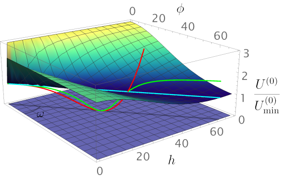
Figure 1: The normalized tree-level potential $U^{(0)}(\phi,h)/U^{(0)}_{\rm min}$ (3.1) and its flat direction (cyan line). We also plot the normalized one-loop corrected potential along the flat direction $U_{\rm eff}(s_{c})/U_{\rm eff}(0)$ (3.22) (red curve) and the normalized inflaton potential $\bar{U}(s_{c})/\bar{U}(0)$ (4.18) (green curve). The values of the parameters are $\tilde{\alpha}=10^{9},\,\xi_{s}=10^{-3},\,$ and $\mathcal{M}\simeq 0.0357$. For illustrative purposes we have chosen the values of the couplings $\lambda_{\phi},\,\lambda_{h},\,\lambda_{h\phi}$ such that the mixing angle (3.7) has the unrealistic value of $\omega\simeq 0.732$.

In the end, having started with a general scale invariant action which involves adimensional matter-gravity and matter-matter couplings, we have obtained an action with a noncanonical scalar field that is minimally coupled to the usual Einstein-Hilbert action at the expense of negligible higher-order kinetic terms and a modified potential, which as we will see next is suitable for successful inflation in accordance with observations.

5 Slow roll approximation and contact with observations

In this section, in order to constrain the parametric space of our model, we compare its predictions for the cosmological observables with their corresponding latest observational bounds as set by the Planck collaboration.

5.1 Inflationary observables and number of $e$-folds

The number of $e$-folds elapsed during the inflationary phase can be obtained in terms of the potential $\bar{U}(s_{c})$ and the kinetic term coupling function $K(s_{c})$ as

$$N_{\star}\equiv N(s_{c\star})=\int_{s_{c,\rm end}}^{s_{c\star}}{K(s_{c})\frac{\bar{U}(s_{c})}{\bar{U}^{\prime}(s_{c})}}\differential s_{c}\,,$$ (5.1)

where primes are used to denote differentiation with respect to the argument, while the subscripts $``\star"$ and $``{\rm end}"$ denote quantities at the time of horizon crossing of the pivot scale $k_{\star}$, and at the end of inflation respectively. The potential slow roll parameters (PSRPs) are defined as

$$\epsilon(s_{c})\equiv\frac{1}{2K(s_{c})}\left[\frac{\bar{U}^{\prime}(s_{c})}{\bar{U}(s_{c})}\right]^{2}\,,\quad\eta(s_{c})\equiv\frac{1}{\bar{U}(s_{c})\sqrt{K(s_{c})}}\left[\frac{\bar{U}^{\prime}(s_{c})}{\sqrt{K(s_{c})}}\right]^{\prime}\,.$$ (5.2)

During slow roll inflation $\epsilon(s_{c})\ll 1$ and $|\eta(s_{c})|\ll 1$ and inflation ends, to a very good approximation, when $\epsilon(s_{c})=1$. The values of the cosmological observables in the slow roll approximation can be obtained in terms of the PSRPs evaluated at the time of horizon crossing $\epsilon_{\star}\equiv\epsilon(s_{c\star})$ and $\eta_{\star}\equiv\eta(s_{c\star})$. The observables that are relevant for our analysis are the tensor-to-scalar ratio

$$r\simeq 16\,\epsilon_{\star}\,,$$ (5.3)

the tilt of the scalar power spectrum

$$n_{s}\simeq 1-6\,\epsilon_{\star}+2\,\eta_{\star}\,,$$ (5.4)

and the amplitude of scalar perturbations

$$A_{s}\simeq\frac{1}{24\pi^{2}}\frac{\bar{U}(s_{c\star})}{\epsilon_{\star}}\,.$$ (5.5)

The Planck collaboration [6] has set the following bounds on the values of the observables:

$$A_{s}\simeq 2.1\times 10^{-9},\qquad\quad n_{s}=\left\{\begin{matrix}\left(0.9607,0.9691\right),&\ 1\sigma\text{ region}\\ \left(0.9565,0.9733\right),&\ 2\sigma\text{ region}\end{matrix}\right.,\qquad\quad r\lesssim 0.056\,.$$ (5.6)

The number of $e$-folds at the pivot scale $k_{\star}$ assuming instantaneous reheating can be very well approximated as [6, 225]

$$N_{\star}=\ln\left[\left(\frac{\pi^{2}}{30}\right)^{\frac{1}{4}}\frac{(g_{s,0})^{\frac{1}{3}}}{\sqrt{3}}\frac{T_{0}}{H_{0}}\right]-\ln\left[\frac{k_{\star}}{a_{0}H_{0}}\right]+\frac{1}{4}\ln\left[\frac{\bar{U}^{2}(s_{c\star})}{\rho_{\rm end}}\right]-\frac{1}{12}\ln\left[g_{s,{\rm reh}}\right]\,,$$ (5.7)

where the subscripts $``0"$ and $``{\rm reh}"$ denote quantities at the present epoch and reheating phase respectively. With $\rho$ we denote the energy density. The entropy density degrees of freedom $g_{s}$ have the values $g_{s,0}=43/11$ and $g_{s,{\rm reh}}=\mathcal{O}(100)$ in our model and for reheating temperatures $\sim 1\,\mathrm{TeV}$ or higher. At the present epoch the CMB temperature and the Hubble constant are $T_{0}=2.725\,\mathrm{K}$ and $H_{0}=67.6\,\mathrm{km/s/Mpc}$ respectively and we fix the pivot scale to $k_{\star}=0.002\,\text{Mpc}^{-1}$. Being more accurate we should calculate $\rho_{\rm end}$ by taking into account that the Hubble slow roll parameter $\epsilon_{1}\equiv-\dot{H}/H^{2}$ is exactly $\epsilon_{1}=1$ at the end of inflation. This condition gives that $\rho_{\rm end}=3\bar{U}(s_{c,\rm end})/2$. Using this and writing (5.7) in terms of the potential (3.22) we can make explicit the dependence of the number of $e$-folds on the parameter $\tilde{\alpha}$, that is,

$$N_{\star}=64.3+\frac{1}{4}\ln\left(\frac{2{U_{\rm eff}^{\star}}^{2}(1+\tilde{\alpha}U_{\rm eff}^{\rm end})}{3U_{\rm eff}^{\rm end}(1+\tilde{\alpha}U_{\rm eff}^{\star})^{2}}\right)\,.$$ (5.8)

In [131, 69], the higher-order kinetic terms appearing in the action (4.17) have been taken into account in the calculation of $\rho_{\rm end}$, but as it is shown there, only an insignificant correction arises in the numerical factor of the number of $e$-folds. In addition, in [131, 140] the reheating mechanism in $R^{2}$ Palatini inflationary models has been studied, but beyond the case of instantaneous reheating, allowing a wider range for the number of $e$-folds for various values of the equation of state parameter.

5.2 Small and large field inflation

Prior to performing the full parametric space investigation for the inflationary predictions of the model, we mention some asymptotic limits with respect to the value of the effective nonminimal coupling $\xi_{s}$. For $\xi_{s}\ll 1$ and $\tilde{\alpha}=0$ we find that the predictions for both small field inflation (SFI) and large field inflation (LFI) correspond to those of quadratic inflation,

$$n_{s}\simeq 1-\frac{2}{N_{\star}}\,,\qquad r_{0}\simeq\frac{8}{N_{\star}}\,,$$ (5.9)

where $r_{0}$ denotes the tensor-to-scalar ratio for $\tilde{\alpha}=0$. On the other hand, for $\xi_{s}\gg 1$ we find

$$n_{s}\simeq 1-\frac{3}{N_{\star}}\,,$$ (5.10)

for both SFI and LFI, while

$$r_{0}\simeq\frac{16}{N_{\star}}\,\quad\text{(for LFI)}\,,\qquad r_{0}\simeq 0\,\quad\text{(for SFI)\,,}$$ (5.11)

Note that the first limit corresponds to the prediction of quartic inflation. When $\tilde{\alpha}\neq 0$, the predictions for $n_{s}$ remain the same but $r$ gets modified as [124, 69]

$$r=\frac{r_{0}}{1+\tilde{\alpha}U^{\star}_{\rm eff}}=\frac{r_{0}}{1+\frac{3}{2}\pi^{2}\tilde{\alpha}A_{s}r_{0}}\,,$$ (5.12)

therefore, the presence of the parameter $\tilde{\alpha}$ results in a suppression of the value of tensor-to-scalar ratio.

Let us now turn to the full analysis of the parametric space of our model with respect to its predictions for the cosmological observables. For each given set of values for the parameters $\tilde{\alpha}$ and $\xi_{\rm s}$, we have employed Eq. (5.8) to obtain the number of $e$-folds that complies with the constraints from reheating, while the value of $\mathcal{M}$ has been fixed in each case such that we always have $A_{s}=2.1\times 10^{-9}$ at $k_{\star}=0.05\,\text{Mpc}^{-1}$ in accordance with the bounds set by the Planck collaboration. For both SFI and LFI, we have considered various values of $\tilde{\alpha}$ and a wide range of values for $\xi_{\rm s}$ ranging from $\xi_{\rm s}\ll 1$ to $\xi_{\rm s}\gg 1$ and in Fig. 2 we plot the corresponding predictions for the tensor-to-scalar ratio and the scalar tilt against the $68\%$ (dark blue) and $95\%$ (light blue) CL regions for $n_{\rm s}$ and $r$ at $k_{*}=0.002\,\text{Mpc}^{-1}$ as obtained with the combined data from Planck+BK15+BAO [6].

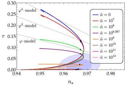
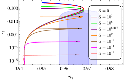
Figure 2: The predictions for the tensor-to-scalar ratio ($r$) and the tilt of the scalar spectrum ($n_{\rm s}$) as $\xi_{\rm s}$ ranges from $\xi_{\rm s}\ll 1$ to $\xi_{\rm s}\gg 1$ for various values of $\tilde{\alpha}$. For each one of the curves, the black dot corresponds to the $\xi_{\rm s}\rightarrow 0$ limit (see Table 2) and $\xi_{\rm s}$ increases monotonically as we move away from it along each one of the two directions on the curve. The upper (lower) part of a curve with respect to its $\xi_{\rm s}\rightarrow 0$ limit, corresponds to the predictions of large (small) field inflation. On the left (right) panel, the predictions are depicted in linear (logarithmic) scale.

The different curves correspond to fixed values of $\tilde{\alpha}$, while $\xi_{\rm s}$ ranges along the curves with the black dot on each curve corresponding to the $\xi_{\rm s}\rightarrow 0$ limit. These dots also designate the transition point between the predictions of SFI and LFI with the lower (upper) part of each curve corresponding to small (large) field inflation. Evidently in the limit of small $\xi_{\rm s}$ the predictions of SFI and LFI are identical. As we move away from the $\xi_{\rm s}\rightarrow 0$ limit along a given curve in both directions $\xi_{\rm s}$ increases monotonically with the top end of the curves corresponding to $\xi_{\rm s}$ values of $\mathcal{O}\left(10^{8}\right)$ and the bottom end (more clearly shown in the right panel of Fig. 2) to values of $\mathcal{O}\left(10^{-1}\right)$.

$\tilde{\alpha}$	$0$	$10^{7}$	$10^{8}$	$1.85\times 10^{8}$	$10^{9}$	$10^{10}$	$10^{11}$	$10^{12}$
$r$	0.13090	0.12526	0.09022	0.07134	0.02368	0.00282	0.00029	0.00003
$n_{s}$	0.96727	0.96726	0.96717	0.96711	0.96681	0.96621	0.96563	0.96517
$N_{\star}$	60.6	60.6	60.4	60.3	59.8	58.8	58.0	57.3

Table 2: The predicted values for the tensor-to-scalar ratio ($r$), tilt of the scalar spectrum ($n_{\rm s}$) and number of efolds ($N_{\star}$), in the limit $\xi_{\rm s}\rightarrow 0$ for various values of $\tilde{\alpha}$.

The effect of $\tilde{\alpha}$ on the inflationary predictions is to suppresses the value of $r$ (cf. Eq. (5.12)). This effect becomes important for values $\tilde{\alpha}\gtrsim 10^{6}-10^{7}$. As the right panel of Fig. 2 reveals, for sufficiently large values of $\tilde{\alpha}$ the predictions of SFI and LFI are identical along an extended range of values of $\xi_{\rm s}$. This can be understood via the shape of the inflationary potential that becomes symmetric about the location of the VEV for $\tilde{\alpha}\gg 1$, see Fig. 3.

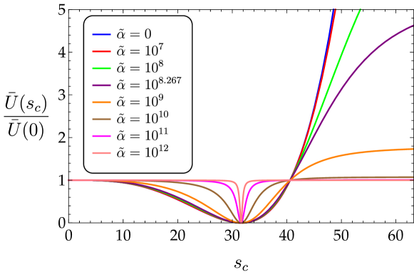
Figure 3: The normalized potential $\bar{U}(s_{c})$ for $\xi_{\rm s}=0.001$ and various values of $\tilde{\alpha}$. In the limit $\tilde{\alpha}\gg 1$, the potential becomes symmetric about its VEV and consequently the predictions for small and large field inflation are identical.

A further inspection of Fig. 2 reveals that for values of $\tilde{\alpha}\lesssim 10^{8.267}\simeq 1.85\times 10^{8}$, LFI is not viable since its predictions lay outside the $95\%$ CL region for the measured values for $r$ and $n_{s}$. On the other hand, SFI complies with observations for a finite range of values of $\xi_{\rm s}$ with the smallest (largest) viable value of $\xi_{\rm s}$ yielding the largest (smallest) predicted value for $r$ for a given $\tilde{\alpha}$, see also Table 3. This range is $2\times 10^{-4}\lesssim\xi_{s}\lesssim 4\times 10^{-3}$ and consequently, via (3.23) the VEV of the inflaton is restricted to $15\,M_{\rm P}\lesssim v_{s}\lesssim 70\,M_{\rm P}$. Furthermore, the finite range of allowed values for $\xi_{\rm s}$ implies a corresponding finite range of viable values for the parameter $\mathcal{M}$ as can be seen in Fig. 4.

Small field inflation
$\tilde{\alpha}$	$\xi_{\rm s}^{\rm(min)}$	$\mathcal{M}$	$r$	$n_{s}$	$N_{\star}$
$0$	$0.0006267$	$0.0502432$	$0.0729636$	$0.968159$	$60.3$
$10^{7}$	$0.0005830$	$0.0510926$	$0.0730490$	$0.968233$	$60.3$
$10^{8}$	$0.0002017$	$0.0651665$	$0.0732724$	$0.968439$	$60.3$
$\tilde{\alpha}$	$\xi_{\rm s}^{\rm(max)}$	$\mathcal{M}$	$r$	$n_{s}$	$N_{\star}$
$0$	$0.0041417$	$0.0297085$	$0.0161109$	$0.957741$	$59.6$
$10^{7}$	$0.0041389$	$0.0297168$	$0.0160355$	$0.957747$	$59.6$
$10^{8}$	$0.0041367$	$0.0297308$	$0.0152745$	$0.957739$	$59.6$

Table 3: For $\tilde{\alpha}\lesssim 10^{8.267}\simeq 1.85\times 10^{8}$, only small field inflation yields viable values for $r$ and $n_{s}$ (see Fig. 2). Here, we give the minimum and maximum values of $\xi_{\rm s}$ for which we obtain viable predictions for various $\tilde{\alpha}$. We also give the values of $\mathcal{M}$, $r$, $n_{s}$ and $N_{\star}$ for these marginal values of $\xi_{\rm s}$.

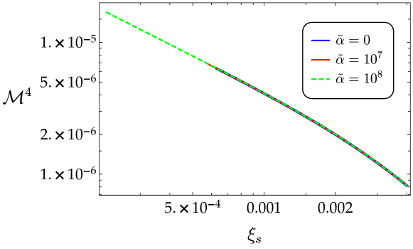
Figure 4: The parameter $\mathcal{M}^{4}$ as a function of $\xi_{\rm s}$, for the viable range of values for $\xi_{\rm s}$ as given in Table 3 for small field inflation. For $\tilde{\alpha}\gtrsim 10^{8.267}\simeq 1.85\times 10^{8}$, the $\xi_{\rm s}\rightarrow 0$ limit is located in the observationally viable $95\%$ CL region of the $r$-$n_{s}$ plot and thus there is no lower cutoff for the value of $\xi_{\rm s}$. Consequently in this case there is no upper cutoff for $\mathcal{M}^{4}$.

For values of $\tilde{\alpha}\gtrsim 10^{8.267}\simeq 1.85\times 10^{8}$ the $\xi_{\rm s}\rightarrow 0$ limit is located within the observationally viable $95\%$ CL region of the $r$-$n_{s}$ plot (see Fig. 2) and so SFI and LFI exhibit only an upper cutoff, $\xi_{s}\lesssim 4\times 10^{-3},$ for the viable values of $\xi_{\rm s}$ as it is shown in Table 4. This in turn implies a lower cutoff, $15\,M_{\rm P}\lesssim v_{s}$, for the VEV of the inflaton.

To summarize, in all the cases $v_{s}$ must be super-Planckian which imposes that $v_{s}\simeq v_{\phi}$ as $v_{h}\sim\mathcal{O}(10^{-16})\,M_{\rm P}$. It is then evident that the mixing angle as defined in Eq. (3.7) will satisfy $\omega\simeq 0$ and thus the flat direction, for values of the parameters that lay in the viable regions of the parametric space, will be nearly identified with the direction of the field $\phi$ in field space, see Fig. 1.

Small field inflation
$\tilde{\alpha}$	$\xi_{\rm s}^{\rm(max)}$	$\mathcal{M}$	$r$	$n_{s}$	$N_{\star}$
$10^{9}$	$0.0040967$	$0.0299033$	$0.0103843$	$0.957734$	$59.4$
$10^{10}$	$0.0039033$	$0.0306853$	$0.0024263$	$0.957835$	$58.8$
$10^{11}$	$0.0036767$	$0.0316817$	$0.0002763$	$0.957919$	$58.0$
$10^{12}$	$0.0035200$	$0.0324432$	$0.0000280$	$0.957921$	$57.3$
Large field inflation
$\tilde{\alpha}$	$\xi_{\rm s}^{\rm(max)}$	$\mathcal{M}$	$r$	$n_{s}$	$N_{\star}$
$10^{9}$	$0.0028733$	$0.0245332$	$0.0248280$	$0.958142$	$60.0$
$10^{10}$	$0.0025667$	$0.0259176$	$0.0027631$	$0.957819$	$59.0$
$10^{11}$	$0.0020250$	$0.0286194$	$0.0002796$	$0.957922$	$58.1$
$10^{12}$	$0.0017108$	$0.0306805$	$0.0000280$	$0.957918$	$57.4$

Table 4: For various $\tilde{\alpha}\gtrsim 10^{8.267}\simeq 1.85\times 10^{8}$, and for both small and large field inflation, we give the corresponding maximum values of $\xi_{\rm s}$ that yield predictions that comply with the observational bounds. We also give the values of $\mathcal{M}$, $r$, $n_{s}$ and $N_{\star}$ for these marginal values of $\xi_{\rm s}$.

6 Conclusions

In this paper we have studied a model of scale-invariant quadratic gravity in the context of the Palatini formulation. The Planck scale is dynamically generated via the Coleman-Weinberg formalism through the VEVs of the scalar field $\phi$ and the Higgs field $h$. These scalar fields were nonminimally coupled to gravity through terms of the form $\xi_{i}\Phi_{i}^{2}R$, where $\Phi_{i}=\phi,h$. The extra scalar field $\phi$ originated from an $U(1)_{X}$ extension of the SM containing an extra gauge boson $X_{\mu}$ and three right-handed neutrinos $N^{i}_{R}$. The Higgs mass was generated through the portal coupling $\lambda_{h\phi}h^{2}\phi^{2}$. This is exactly the significance of the addition of the extra scalar field $\phi$. Without it, the necessity of the existence of a Higgs mass term with a dimensionful coupling would have broken the scale invariance of our model. A possible extra $Z_{2}$ symmetry facilitates the stability of the potential dark matter candidates in the context of our model. As discussed, these can be either the new fermions of the model e.g. the right-handed neutrinos or the extra Dirac fermion $\zeta$, or the extra $U(1)_{X}$ gauge boson.

We have employed the Gildener-Weinberg approach, the generalization of the Coleman-Weinberg mechanism to the multiple fields case, in order to identify the flat direction of the tree-level potential. Along the flat direction, the theory effectively becomes single field and by computing the quantum corrections we obtain the one-loop effective potential, which is stabilized due to the extra $U(1)_{X}$ gauge boson. In the effective single-field description, two parameters are important for our analysis namely the effective nonminimal coupling $\xi_{s}$, which is constructed out of the nonminimal couplings of $\phi$ and $h$ and their mixing angle $\omega$, and the effective higher-curvature coupling $\tilde{\alpha}$ which corresponds to a combination of the coupling constants of the quadratic curvature corrections in the action. These quadratic in curvature terms are the usual scale invariant terms $R^{2}$ and $R_{(\mu\nu)}R^{(\mu\nu)}$. The fact that their effect on the inflationary observables can be described collectively by the common coupling $\tilde{\alpha}$ reveals that their contribution to the final EF potential is the same. On the other hand, the higher order kinetic terms generated in the EF are not of the same form, as the $R^{2}$ term gives us only a second order kinetic term, while the $R_{(\mu\nu)}R^{(\mu\nu)}$ term gives higher than the second order terms. The study of such kinetic terms was out of the scope of this paper as they are negligible at least during slow roll.

In order to transform the action into the EF and compare the predictions of the model with observations, the use of both conformal and disformal transformations is required. The one-loop corrections are taken in the “intermediate frame”, that is after having performed the conformal transformation that decouples the scalar fields from the Einstein-Hilbert term, but before the disformal transformation that removes the quadratic curvature terms from the gravity sector. It is in this intermediate frame that we may have a one-loop effective potential with a minimum at zero without invoking a cosmological constant term that would render our model “quasi scale invariant”. Upon recasting the action to the EF, we end up with a modified effective potential $\bar{U}(s_{c})$ in terms of a canonical scalar field $s_{c}$ that plays the role of the inflaton. The shape of the potential $\bar{U}(s_{c})$ exhibits plateaus on both sides of the minimum and thus both small field inflation (SFI) and large field inflation (LFI) can be accommodated in our model. The additional higher-order kinetic terms that arise in the EF are negligible in the slow roll approximation, and so we have retained only linear order terms in our analysis. Applying the cosmological data on inflation we were able to constrain the size of the VEV of these scalar fields, and consequently the masses of the extra gauge boson and the right-handed neutrinos.

In order to constrain the parametric space we have considered the latest bounds on cosmological observables as set by the Planck collaboration and we have found that our model complies with observations for a wide range of parameters. More precisely, for values of the parameter $\tilde{\alpha}$ in the range $\tilde{\alpha}\gtrsim 1.85\times 10^{8}$, both SFI and LFI support viable inflation when $\xi_{s}\lesssim\mathcal{O}(10^{-3})$. In the large $\tilde{\alpha}$ limit, the inflationary potential becomes symmetric about its minimum and consequently the predictions for the observables of SFI and LFI are identical.

When $\tilde{\alpha}\lesssim 1.85\times 10^{8}$, and independently of the value of $\xi_{s}$, LFI is nonviable since the predicted values for the tensor-to-scalar ratio and the tilt of the scalar power spectrum lay outside the $95\%$ CL region. On the other hand, SFI exhibits regions in the parametric space that are viable for any $\tilde{\alpha}$ with $\xi_{s}$ interpolating between a maximum and a minimum value. Eventually, the largest viable value for $\xi_{s}$ in our model is obtained within the context of SFI and is approximately $\xi_{s}\simeq 4\times 10^{-3}$ which translates to a minimum value for the VEV of $s_{c}$ in the vicinity of $15\,M_{\rm P}$. It will be interesting to investigate whether the rest of the shortcomings of the SM, such as the strong CP problem, can be addressed in a similar setting where successful inflation can be realized and the dark matter and baryon asymmetry problems can be solved in a common framework.

Appendix A Details on the variations

Substituting (4.2) in (4.5) gives us that the auxiliary field $\Sigma_{\mu\nu}$ in terms of $q_{\mu\nu}$ and $g_{\mu\nu}$ reads

$$\Sigma_{\mu\nu}=\frac{1}{2\beta}\frac{\sqrt{-q}}{\sqrt{-g}}q^{\kappa\lambda}g_{\kappa\mu}g_{\lambda\nu}-\frac{1}{2\beta+8\alpha}\left(1+\frac{\alpha}{\beta}\frac{\sqrt{-q}}{\sqrt{-g}}q^{\kappa\lambda}g_{\kappa\lambda}\right)g_{\mu\nu}\,,$$ (A.1)

and its trace is

$$\Sigma=g^{\mu\nu}\Sigma_{\mu\nu}=\frac{-4}{2\beta+8\alpha}+\frac{1}{2\beta+8\alpha}\frac{\sqrt{-q}}{\sqrt{-g}}q^{\kappa\lambda}g_{\kappa\lambda}\,.$$ (A.2)

The part of the Lagrangian density that has to be varied with respect to $g_{\mu\nu}$ is

$$\sqrt{-g}\mathcal{L}_{g} = -\sqrt{-g}\left(\frac{1}{2}\frac{\partial C}{\partial\Sigma_{\mu\nu}}\Sigma_{\mu\nu}-\frac{1}{2}C-\mathcal{L}_{m}\right)$$ (A.3)

$$= -\sqrt{-g}\left(\frac{\alpha}{2}\Sigma^{2}+\frac{\beta}{2}\Sigma_{\mu\nu}\Sigma^{\mu\nu}+\frac{1}{2}g^{\mu\nu}\partial_{\mu}s_{c}\partial_{\nu}s_{c}+U_{\rm eff}(s_{c})\right)\,.$$

Varying (A.3) we obtain that

$$\delta\left(\sqrt{-g}\mathcal{L}_{g}\right) = -\sqrt{-g}\bigg{[}\alpha\Sigma\delta\Sigma+\beta g^{\mu\gamma}\Sigma_{\mu\nu}\delta\left(g^{\rho\nu}\Sigma_{\gamma\rho}\right)+\frac{1}{2}\partial_{\mu}s_{c}\partial_{\nu}s_{c}\delta g^{\mu\nu}\bigg{]}$$ (A.4)

$$-\frac{1}{2}\sqrt{-g}g_{\mu\nu}\delta g^{\mu\nu}\bigg{[}-\frac{\alpha}{2}\Sigma^{2}-\frac{\beta}{2}\Sigma_{\mu\nu}\Sigma^{\mu\nu}-U_{\rm eff}(s_{c})-\frac{1}{2}g^{\kappa\lambda}\partial_{\kappa}s_{c}\partial_{\lambda}s_{c}\bigg{]}\,.$$

Substituting (A.1) and (A.2) in (A.4) and after manipulations we have that

$$\frac{1}{\sqrt{-g}}\frac{\delta S}{\delta g^{\mu\nu}}= -\frac{1}{4(\beta+4\alpha)}\frac{\sqrt{-q}}{\sqrt{-g}}q^{\sigma\lambda}g_{\sigma\mu}g_{\lambda\nu}$$ (A.5)

$$+\frac{1}{4\beta}\frac{q}{g}\left(q^{\sigma\lambda}q^{\rho\delta}g_{\lambda\delta}g_{\rho\nu}g_{\sigma\mu}-\frac{\alpha}{\beta+4\alpha}q^{\delta\rho}g_{\delta\rho}q^{\sigma\lambda}g_{\sigma\mu}g_{\lambda\nu}\right)$$

$$+\frac{1}{2}g_{\mu\nu}\left[\frac{1}{\beta+4\alpha}\left(\frac{1}{2}+\frac{\alpha}{8\beta}\frac{q}{g}q^{\lambda\sigma}g_{\lambda\sigma}q^{\rho\delta}g_{\rho\delta}\right)-\frac{q}{g}\frac{1}{8\beta}q^{\lambda\sigma}q^{\delta\rho}g_{\lambda\delta}g_{\sigma\rho}\right]$$

$$+\frac{1}{2}g_{\mu\nu}\left(\frac{1}{2}g^{\lambda\sigma}\partial_{\lambda}s_{c}\partial_{\sigma}s_{c}+U_{\rm eff}(s_{c})\right)-\frac{1}{2}\partial_{\mu}s_{c}\partial_{\nu}s_{c}=0\,.$$

Appendix B The functions $R_{i}$, $a_{i}$, and $b_{i}$

The functions $R_{i}$ which have been displayed in Eqs. (4.14)-(4.15) are listed below

$$R_{1} = B\left(2A-2BX_{q}\right)\,,$$

$$R_{2} = 4A-2BX_{q}\,,$$

$$R_{3} = 4A^{2}-4ABX_{q}+4B^{2}X_{q}^{2}\,,$$

$$R_{4} = A(R_{1}+AB)-2BR_{1}X_{q}\,,$$

$$R_{5} = A^{3}\left(A-2BX_{q}\right)\,.$$ (B.1)

The coefficients $a_{i}$, and $b_{i}$ which have been displayed in Eq. (4.16) are

$$a_{0} = \frac{1}{1+\tilde{\alpha}U_{\rm eff}}\,,$$

$$b_{0} = \frac{(\tilde{\beta}-\tilde{\alpha})}{(1+\tilde{\alpha}U_{\rm eff})(1+\tilde{\beta}U_{\rm eff})}\,,$$

$$a_{1} = \frac{\tilde{\beta}}{2(1+\tilde{\beta}U_{\rm eff})}\,,$$

$$b_{1} = \frac{(\tilde{\beta}-\tilde{\alpha})\left(3\tilde{\beta}-2\tilde{\alpha}+(2\tilde{\beta}-\tilde{\alpha})(\tilde{\alpha}+\tilde{\beta})U_{\rm eff}+\tilde{\alpha}\tilde{\beta}^{2}U_{\rm eff}^{2}\right)}{(1+\tilde{\alpha}U_{\rm eff})(1+\tilde{\beta}U_{\rm eff})^{3}}\,,$$ (B.2)

where we have defined $\tilde{\alpha}=2\beta+8\alpha$, $\tilde{\beta}=4\beta+8\alpha$ and $U_{\rm eff}=U_{\rm eff}(s_{c})$. As it seems, for $\tilde{\alpha}=\tilde{\beta}$, the coefficients $b_{0}$ and $b_{1}$, like the rest higher order $b$ coefficients of the same series (4.16), are equal to zero. This is expected, as the equality of the tilted factors is translated to an elimination of the $R_{\mu\nu}R^{\mu\nu}$ term and so the disformal transformation is reduced again to the usual conformal.

References

- [1] Planck Collaboration, N. Aghanim et al., Planck 2018 results. VI. Cosmological parameters, Astron. Astrophys. 641 (2020) A6, [arXiv:1807.06209].
- [2] A. A. Starobinsky, A New Type of Isotropic Cosmological Models Without Singularity, Phys. Lett. 91B (1980) 99–102.
- [3] A. H. Guth, The Inflationary Universe: A Possible Solution to the Horizon and Flatness Problems, Phys. Rev. D23 (1981) 347–356.
- [4] A. D. Linde, A New Inflationary Universe Scenario: A Possible Solution of the Horizon, Flatness, Homogeneity, Isotropy and Primordial Monopole Problems, Phys. Lett. 108B (1982) 389–393.
- [5] A. Albrecht and P. J. Steinhardt, Cosmology for Grand Unified Theories with Radiatively Induced Symmetry Breaking, Phys. Rev. Lett. 48 (1982) 1220–1223.
- [6] Planck Collaboration, Y. Akrami et al., Planck 2018 results. X. Constraints on inflation, Astron. Astrophys. 641 (2020) A10, [arXiv:1807.06211].
- [7] V. Faraoni, E. Gunzig, and P. Nardone, Conformal transformations in classical gravitational theories and in cosmology, Fund. Cosmic Phys. 20 (1999) 121, [gr-qc/9811047].
- [8] V. Faraoni, Cosmology in scalar tensor gravity. 2004.
- [9] E. E. Flanagan, The Conformal frame freedom in theories of gravitation, Class. Quant. Grav. 21 (2004) 3817, [gr-qc/0403063].
- [10] L. Jarv, P. Kuusk, and M. Saal, Scalar-tensor cosmology at the general relativity limit: Jordan versus Einstein frame, Phys. Rev. D 76 (2007) 103506, [arXiv:0705.4644].
- [11] T. Chiba and M. Yamaguchi, Conformal-Frame (In)dependence of Cosmological Observations in Scalar-Tensor Theory, JCAP 10 (2013) 040, [arXiv:1308.1142].
- [12] M. Postma and M. Volponi, Equivalence of the Einstein and Jordan frames, Phys. Rev. D 90 (2014), no. 10 103516, [arXiv:1407.6874].
- [13] L. Järv, P. Kuusk, M. Saal, and O. Vilson, Invariant quantities in the scalar-tensor theories of gravitation, Phys. Rev. D 91 (2015), no. 2 024041, [arXiv:1411.1947].
- [14] L. Järv, P. Kuusk, M. Saal, and O. Vilson, Transformation properties and general relativity regime in scalar–tensor theories, Class. Quant. Grav. 32 (2015) 235013, [arXiv:1504.02686].
- [15] P. Kuusk, M. Rünkla, M. Saal, and O. Vilson, Invariant slow-roll parameters in scalar–tensor theories, Class. Quant. Grav. 33 (2016), no. 19 195008, [arXiv:1605.07033].
- [16] L. Järv, K. Kannike, L. Marzola, A. Racioppi, M. Raidal, M. Rünkla, M. Saal, and H. Veermäe, Frame-Independent Classification of Single-Field Inflationary Models, Phys. Rev. Lett. 118 (2017), no. 15 151302, [arXiv:1612.06863].
- [17] A. Karam, T. Pappas, and K. Tamvakis, Frame-dependence of higher-order inflationary observables in scalar-tensor theories, Phys. Rev. D 96 (2017), no. 6 064036, [arXiv:1707.00984].
- [18] D. Burns, S. Karamitsos, and A. Pilaftsis, Frame-Covariant Formulation of Inflation in Scalar-Curvature Theories, Nucl. Phys. B907 (2016) 785–819, [arXiv:1603.03730].
- [19] S. Karamitsos and A. Pilaftsis, On the Cosmological Frame Problem, PoS CORFU2017 (2018) 036, [arXiv:1801.07151].
- [20] L. Järv, A. Karam, A. Kozak, A. Lykkas, A. Racioppi, and M. Saal, Equivalence of inflationary models between the metric and Palatini formulation of scalar-tensor theories, Phys. Rev. D 102 (2020), no. 4 044029, [arXiv:2005.14571].
- [21] I. D. Gialamas, A. Karam, A. Lykkas, and T. D. Pappas, Palatini-Higgs inflation with nonminimal derivative coupling, Phys. Rev. D 102 (2020), no. 6 063522, [arXiv:2008.06371].
- [22] A. Karam, S. Karamitsos, and M. Saal, -function reconstruction of Palatini inflationary attractors, arXiv:2103.01182.
- [23] M. Shaposhnikov and D. Zenhausern, Scale invariance, unimodular gravity and dark energy, Phys. Lett. B671 (2009) 187–192, [arXiv:0809.3395].
- [24] J. Garcia-Bellido, J. Rubio, M. Shaposhnikov, and D. Zenhausern, Higgs-Dilaton Cosmology: From the Early to the Late Universe, Phys. Rev. D 84 (2011) 123504, [arXiv:1107.2163].
- [25] F. Bezrukov, G. K. Karananas, J. Rubio, and M. Shaposhnikov, Higgs-Dilaton Cosmology: an effective field theory approach, Phys. Rev. D 87 (2013), no. 9 096001, [arXiv:1212.4148].
- [26] V. V. Khoze, Inflation and Dark Matter in the Higgs Portal of Classically Scale Invariant Standard Model, JHEP 1311 (2013) 215, [arXiv:1308.6338].
- [27] T. G. Steele, Z.-W. Wang, D. Contreras, and R. B. Mann, Viable dark matter via radiative symmetry breaking in a scalar singlet Higgs portal extension of the standard model, Phys. Rev. Lett. 112 (2014), no. 17 171602, [arXiv:1310.1960].
- [28] J. Ren, Z.-Z. Xianyu, and H.-J. He, Higgs Gravitational Interaction, Weak Boson Scattering, and Higgs Inflation in Jordan and Einstein Frames, JCAP 06 (2014) 032, [arXiv:1404.4627].
- [29] K. Kannike, A. Racioppi, and M. Raidal, Embedding inflation into the Standard Model - more evidence for classical scale invariance, JHEP 1406 (2014) 154, [arXiv:1405.3987].
- [30] C. Csaki, N. Kaloper, J. Serra, and J. Terning, Inflation from Broken Scale Invariance, Phys. Rev. Lett. 113 (2014) 161302, [arXiv:1406.5192].
- [31] K. Kannike, G. Hütsi, L. Pizza, A. Racioppi, M. Raidal, et al., Dynamically Induced Planck Scale and Inflation, JHEP 1505 (2015) 065, [arXiv:1502.01334].
- [32] K. Kannike, A. Racioppi, and M. Raidal, Linear inflation from quartic potential, JHEP 01 (2016) 035, [arXiv:1509.05423].
- [33] Z.-W. Wang, T. G. Steele, T. Hanif, and R. B. Mann, Conformal Complex Singlet Extension of the Standard Model: Scenario for Dark Matter and a Second Higgs Boson, JHEP 08 (2016) 065, [arXiv:1510.04321].
- [34] A. Barvinsky, A. Y. Kamenshchik, and D. Nesterov, Origin of inflation in CFT driven cosmology: -gravity and non-minimally coupled inflaton models, Eur. Phys. J. C 75 (2015), no. 12 584, [arXiv:1510.06858].
- [35] A. Farzinnia and S. Kouwn, Classically scale invariant inflation, supermassive WIMPs, and adimensional gravity, Phys. Rev. D 93 (2016), no. 6 063528, [arXiv:1512.05890].
- [36] M. Rinaldi and L. Vanzo, Inflation and reheating in theories with spontaneous scale invariance symmetry breaking, Phys. Rev. D94 (2016), no. 2 024009, [arXiv:1512.07186].
- [37] L. Marzola, A. Racioppi, M. Raidal, F. R. Urban, and H. Veermäe, Non-minimal CW inflation, electroweak symmetry breaking and the 750 GeV anomaly, JHEP 03 (2016) 190, [arXiv:1512.09136].
- [38] N. D. Barrie, A. Kobakhidze, and S. Liang, Natural Inflation with Hidden Scale Invariance, Phys. Lett. B756 (2016) 390–393, [arXiv:1602.04901].
- [39] P. G. Ferreira, C. T. Hill, and G. G. Ross, Scale-Independent Inflation and Hierarchy Generation, Phys. Lett. B 763 (2016) 174–178, [arXiv:1603.05983].
- [40] K. Kannike, A. Racioppi, and M. Raidal, Super-heavy dark matter – Towards predictive scenarios from inflation, Nucl. Phys. B918 (2017) 162–177, [arXiv:1605.09378].
- [41] L. Marzola and A. Racioppi, Minimal but non-minimal inflation and electroweak symmetry breaking, JCAP 1610 (2016), no. 10 010, [arXiv:1606.06887].
- [42] G. K. Karananas and J. Rubio, On the geometrical interpretation of scale-invariant models of inflation, Phys. Lett. B761 (2016) 223–228, [arXiv:1606.08848].
- [43] G. Tambalo and M. Rinaldi, Inflation and reheating in scale-invariant scalar-tensor gravity, Gen. Rel. Grav. 49 (2017), no. 4 52, [arXiv:1610.06478].
- [44] K. Kannike, M. Raidal, C. Spethmann, and H. Veermäe, The evolving Planck mass in classically scale-invariant theories, JHEP 04 (2017) 026, [arXiv:1610.06571].
- [45] M. Artymowski and A. Racioppi, Scalar-tensor linear inflation, JCAP 1704 (2017), no. 04 007, [arXiv:1610.09120].
- [46] P. G. Ferreira, C. T. Hill, and G. G. Ross, Weyl Current, Scale-Invariant Inflation and Planck Scale Generation, Phys. Rev. D 95 (2017), no. 4 043507, [arXiv:1610.09243].
- [47] A. Salvio, Inflationary Perturbations in No-Scale Theories, Eur. Phys. J. C77 (2017), no. 4 267, [arXiv:1703.08012].
- [48] A. Karam, T. Pappas, and K. Tamvakis, Frame-dependence of higher-order inflationary observables in scalar-tensor theories, Phys. Rev. D96 (2017), no. 6 064036, [arXiv:1707.00984].
- [49] K. Kaneta, O. Seto, and R. Takahashi, Very low scale Coleman-Weinberg inflation with non-minimal coupling, Phys. Rev. D97 (2018), no. 6 063004, [arXiv:1708.06455].
- [50] A. Karam, L. Marzola, T. Pappas, A. Racioppi, and K. Tamvakis, Constant-Roll (Quasi-)Linear Inflation, JCAP 05 (2018) 011, [arXiv:1711.09861].
- [51] A. Racioppi, New universal attractor in nonminimally coupled gravity: Linear inflation, Phys. Rev. D 97 (2018), no. 12 123514, [arXiv:1801.08810].
- [52] P. G. Ferreira, C. T. Hill, J. Noller, and G. G. Ross, Inflation in a scale invariant universe, Phys. Rev. D 97 (2018), no. 12 123516, [arXiv:1802.06069].
- [53] D. Benisty and E. I. Guendelman, Two scalar fields inflation from scale-invariant gravity with modified measure, Class. Quant. Grav. 36 (2019), no. 9 095001, [arXiv:1809.09866].
- [54] A. Barnaveli, S. Lucat, and T. Prokopec, Inflation as a spontaneous symmetry breaking of Weyl symmetry, JCAP 01 (2019) 022, [arXiv:1809.10586].
- [55] J. Kubo, M. Lindner, K. Schmitz, and M. Yamada, Planck mass and inflation as consequences of dynamically broken scale invariance, Phys. Rev. D 100 (2019), no. 1 015037, [arXiv:1811.05950].
- [56] S. Mooij, M. Shaposhnikov, and T. Voumard, Hidden and explicit quantum scale invariance, Phys. Rev. D 99 (2019), no. 8 085013, [arXiv:1812.07946].
- [57] M. Shaposhnikov and K. Shimada, Asymptotic Scale Invariance and its Consequences, Phys. Rev. D 99 (2019), no. 10 103528, [arXiv:1812.08706].
- [58] C. Wetterich, Quantum scale symmetry, arXiv:1901.04741.
- [59] S. Vicentini, L. Vanzo, and M. Rinaldi, Scale-invariant inflation with one-loop quantum corrections, Phys. Rev. D 99 (2019), no. 10 103516, [arXiv:1902.04434].
- [60] A. Shkerin, Dilaton-assisted generation of the Fermi scale from the Planck scale, Phys. Rev. D 99 (2019), no. 11 115018, [arXiv:1903.11317].
- [61] P. G. Ferreira, C. T. Hill, J. Noller, and G. G. Ross, Scale-independent inflation, Phys. Rev. D 100 (2019), no. 12 123516, [arXiv:1906.03415].
- [62] D. Ghilencea, Weyl R2 inflation with an emergent Planck scale, JHEP 10 (2019) 209, [arXiv:1906.11572].
- [63] A. Salvio, Quasi-Conformal Models and the Early Universe, Eur. Phys. J. C 79 (2019), no. 9 750, [arXiv:1907.00983].
- [64] I. Oda, Planck Scale from Broken Local Conformal Invariance in Weyl Geometry, Adv. Stud. Theor. Phys. 14 (2020), no. 1-4 9–28, [arXiv:1909.09889].
- [65] A. Racioppi, Non-Minimal (Self-)Running Inflation: Metric vs. Palatini Formulation, JHEP 21 (2021) 011, [arXiv:1912.10038].
- [66] D. Benisty, E. Guendelman, E. Nissimov, and S. Pacheva, Dynamically Generated Inflationary Lambda-CDM, Symmetry 12 (2020), no. 3 481, [arXiv:2002.04110].
- [67] D. Benisty, E. Guendelman, E. Nissimov, and S. Pacheva, Quintessential Inflation with Dynamical Higgs Generation as an Affine Gravity, Symmetry 12 (2020) 734, [arXiv:2003.04723].
- [68] Y. Tang and Y.-L. Wu, Weyl scaling invariant gravity for inflation and dark matter, Phys. Lett. B 809 (2020) 135716, [arXiv:2006.02811].
- [69] I. D. Gialamas, A. Karam, and A. Racioppi, Dynamically induced Planck scale and inflation in the Palatini formulation, JCAP 11 (2020) 014, [arXiv:2006.09124].
- [70] D. M. Ghilencea, Gauging scale symmetry and inflation: Weyl versus Palatini gravity, Eur. Phys. J. C 81 (2021), no. 6 510, [arXiv:2007.14733].
- [71] K. Stelle, Renormalization of Higher Derivative Quantum Gravity, Phys. Rev. D 16 (1977) 953–969.
- [72] T. Biswas, A. Mazumdar, and W. Siegel, Bouncing universes in string-inspired gravity, JCAP 03 (2006) 009, [hep-th/0508194].
- [73] A. Salvio and A. Strumia, Agravity, JHEP 06 (2014) 080, [arXiv:1403.4226].
- [74] A. Edery and Y. Nakayama, Restricted Weyl invariance in four-dimensional curved spacetime, Phys. Rev. D 90 (2014) 043007, [arXiv:1406.0060].
- [75] A. Salvio and A. Strumia, Agravity up to infinite energy, Eur. Phys. J. C78 (2018), no. 2 124, [arXiv:1705.03896].
- [76] A. Salvio, Quadratic Gravity, Front. in Phys. 6 (2018) 77, [arXiv:1804.09944].
- [77] A. Salvio, A. Strumia, and H. Veermäe, New infra-red enhancements in 4-derivative gravity, Eur. Phys. J. C 78 (2018), no. 10 842, [arXiv:1808.07883].
- [78] A. Edery and Y. Nakayama, Critical gravity from four dimensional scale invariant gravity, JHEP 11 (2019) 169, [arXiv:1908.08778].
- [79] A. Salvio and H. Veermäe, Horizonless ultracompact objects and dark matter in quadratic gravity, JCAP 02 (2020) 018, [arXiv:1912.13333].
- [80] D. M. Ghilencea, Palatini quadratic gravity: spontaneous breaking of gauged scale symmetry and inflation, Eur. Phys. J. C 80 (4, 2020) 1147, [arXiv:2003.08516].
- [81] A. Salvio, Dimensional Transmutation in Gravity and Cosmology, Int. J. Mod. Phys. A 36 (2021), no. 08n09 2130006, [arXiv:2012.11608].
- [82] A. Palatini, Deduzione invariantiva delle equazioni gravitazionali dal principio di hamilton, Rendiconti del Circolo Matematico di Palermo (1884-1940) 43 (Dec, 1919) 203–212.
- [83] M. Ferraris, M. Francaviglia, and C. Reina, Variational formulation of general relativity from 1915 to 1925 “palatini’s method” discovered by einstein in 1925, General Relativity and Gravitation 14 (Mar, 1982) 243–254.
- [84] F. Bauer and D. A. Demir, Inflation with Non-Minimal Coupling: Metric versus Palatini Formulations, Phys. Lett. B 665 (2008) 222–226, [arXiv:0803.2664].
- [85] F. Bauer, Filtering out the cosmological constant in the Palatini formalism of modified gravity, Gen. Rel. Grav. 43 (2011) 1733–1757, [arXiv:1007.2546].
- [86] N. Tamanini and C. R. Contaldi, Inflationary Perturbations in Palatini Generalised Gravity, Phys. Rev. D 83 (2011) 044018, [arXiv:1010.0689].
- [87] F. Bauer and D. A. Demir, Higgs-Palatini Inflation and Unitarity, Phys. Lett. B 698 (2011) 425–429, [arXiv:1012.2900].
- [88] S. Rasanen and P. Wahlman, Higgs inflation with loop corrections in the Palatini formulation, JCAP 11 (2017) 047, [arXiv:1709.07853].
- [89] T. Tenkanen, Resurrecting Quadratic Inflation with a non-minimal coupling to gravity, JCAP 12 (2017) 001, [arXiv:1710.02758].
- [90] A. Racioppi, Coleman-Weinberg linear inflation: metric vs. Palatini formulation, JCAP 12 (2017) 041, [arXiv:1710.04853].
- [91] T. Markkanen, T. Tenkanen, V. Vaskonen, and H. Veermäe, Quantum corrections to quartic inflation with a non-minimal coupling: metric vs. Palatini, JCAP 03 (2018) 029, [arXiv:1712.04874].
- [92] L. Järv, A. Racioppi, and T. Tenkanen, Palatini side of inflationary attractors, Phys. Rev. D 97 (2018), no. 8 083513, [arXiv:1712.08471].
- [93] C. Fu, P. Wu, and H. Yu, Inflationary dynamics and preheating of the nonminimally coupled inflaton field in the metric and Palatini formalisms, Phys. Rev. D 96 (2017), no. 10 103542, [arXiv:1801.04089].
- [94] A. Racioppi, New universal attractor in nonminimally coupled gravity: Linear inflation, Phys. Rev. D 97 (2018), no. 12 123514, [arXiv:1801.08810].
- [95] P. Carrilho, D. Mulryne, J. Ronayne, and T. Tenkanen, Attractor Behaviour in Multifield Inflation, JCAP 06 (2018) 032, [arXiv:1804.10489].
- [96] A. Kozak and A. Borowiec, Palatini frames in scalar–tensor theories of gravity, Eur. Phys. J. C 79 (2019), no. 4 335, [arXiv:1808.05598].
- [97] S. Rasanen and E. Tomberg, Planck scale black hole dark matter from Higgs inflation, JCAP 01 (2019) 038, [arXiv:1810.12608].
- [98] S. Rasanen, Higgs inflation in the Palatini formulation with kinetic terms for the metric, Open J. Astrophys. 2 (2019), no. 1 [arXiv:1811.09514].
- [99] J. P. B. Almeida, N. Bernal, J. Rubio, and T. Tenkanen, Hidden Inflaton Dark Matter, JCAP 03 (2019) 012, [arXiv:1811.09640].
- [100] K. Shimada, K. Aoki, and K.-i. Maeda, Metric-affine Gravity and Inflation, Phys. Rev. D 99 (2019), no. 10 104020, [arXiv:1812.03420].
- [101] T. Takahashi and T. Tenkanen, Towards distinguishing variants of non-minimal inflation, JCAP 04 (2019) 035, [arXiv:1812.08492].
- [102] R. Jinno, K. Kaneta, K.-y. Oda, and S. C. Park, Hillclimbing inflation in metric and Palatini formulations, Phys. Lett. B 791 (2019) 396–402, [arXiv:1812.11077].
- [103] J. Rubio and E. S. Tomberg, Preheating in Palatini Higgs inflation, JCAP 04 (2019) 021, [arXiv:1902.10148].
- [104] N. Bostan, Non-minimally coupled quartic inflation with Coleman-Weinberg one-loop corrections in the Palatini formulation, Phys. Lett. B 811 (2020) 135954, [arXiv:1907.13235].
- [105] N. Bostan, Quadratic, Higgs and hilltop potentials in the Palatini gravity, Commun. Theor. Phys. 72 (2020) 085401, [arXiv:1908.09674].
- [106] T. Tenkanen and L. Visinelli, Axion dark matter from Higgs inflation with an intermediate , JCAP 08 (2019) 033, [arXiv:1906.11837].
- [107] T. Tenkanen, Tracing the high energy theory of gravity: an introduction to Palatini inflation, Gen. Rel. Grav. 52 (2020), no. 4 33, [arXiv:2001.10135].
- [108] M. Shaposhnikov, A. Shkerin, and S. Zell, Quantum Effects in Palatini Higgs Inflation, JCAP 07 (2020) 064, [arXiv:2002.07105].
- [109] A. Borowiec and A. Kozak, New class of hybrid metric-Palatini scalar-tensor theories of gravity, JCAP 07 (2020) 003, [arXiv:2003.02741].
- [110] A. Karam, M. Raidal, and E. Tomberg, Gravitational dark matter production in Palatini preheating, JCAP 03 (2021) 064, [arXiv:2007.03484].
- [111] J. McDonald, Does Palatini Higgs Inflation Conserve Unitarity?, JCAP 04 (2021) 069, [arXiv:2007.04111].
- [112] M. Langvik, J.-M. Ojanperä, S. Raatikainen, and S. Räsänen, Higgs inflation with the Holst and the Nieh–Yan term, Phys. Rev. D 103 (2021), no. 8 083514, [arXiv:2007.12595].
- [113] M. Shaposhnikov, A. Shkerin, I. Timiryasov, and S. Zell, Higgs inflation in Einstein-Cartan gravity, JCAP 02 (2021) 008, [arXiv:2007.14978].
- [114] M. Shaposhnikov, A. Shkerin, I. Timiryasov, and S. Zell, Einstein-Cartan gravity, matter, and scale-invariant generalization, JHEP 10 (2020) 177, [arXiv:2007.16158].
- [115] Y. Mikura, Y. Tada, and S. Yokoyama, Conformal inflation in the metric-affine geometry, EPL 132 (2020), no. 3 39001, [arXiv:2008.00628].
- [116] S. Verner, Quintessential Inflation in Palatini Gravity, arXiv:2010.11201.
- [117] V.-M. Enckell, S. Nurmi, S. Räsänen, and E. Tomberg, Critical point Higgs inflation in the Palatini formulation, JHEP 04 (2021) 059, [arXiv:2012.03660].
- [118] Y. Reyimuaji and X. Zhang, Natural inflation with a nonminimal coupling to gravity, JCAP 03 (2021) 059, [arXiv:2012.14248].
- [119] Y. Mikura, Y. Tada, and S. Yokoyama, Minimal -inflation in light of the conformal metric-affine geometry, Phys. Rev. D 103 (2021), no. 10 L101303, [arXiv:2103.13045].
- [120] M. Kubota, K.-Y. Oda, K. Shimada, and M. Yamaguchi, Cosmological Perturbations in Palatini Formalism, JCAP 03 (2021) 006, [arXiv:2010.07867].
- [121] D. Sáez-Chillón Gómez, 3+1 decomposition in modified gravities within the Palatini formalism and some applications, arXiv:2103.16319.
- [122] G. J. Olmo, Palatini Approach to Modified Gravity: f(R) Theories and Beyond, Int. J. Mod. Phys. D 20 (2011) 413–462, [arXiv:1101.3864].
- [123] F. Bombacigno and G. Montani, Big bounce cosmology for Palatini gravity with a Nieh–Yan term, Eur. Phys. J. C 79 (2019), no. 5 405, [arXiv:1809.07563].
- [124] V.-M. Enckell, K. Enqvist, S. Rasanen, and L.-P. Wahlman, Inflation with term in the Palatini formalism, JCAP 02 (2019) 022, [arXiv:1810.05536].
- [125] I. Antoniadis, A. Karam, A. Lykkas, and K. Tamvakis, Palatini inflation in models with an term, JCAP 11 (2018) 028, [arXiv:1810.10418].
- [126] I. Antoniadis, A. Karam, A. Lykkas, T. Pappas, and K. Tamvakis, Rescuing Quartic and Natural Inflation in the Palatini Formalism, JCAP 03 (2019) 005, [arXiv:1812.00847].
- [127] T. Tenkanen, Minimal Higgs inflation with an term in Palatini gravity, Phys. Rev. D 99 (2019), no. 6 063528, [arXiv:1901.01794].
- [128] A. Edery and Y. Nakayama, Palatini formulation of pure gravity yields Einstein gravity with no massless scalar, Phys. Rev. D 99 (2019), no. 12 124018, [arXiv:1902.07876].
- [129] M. Giovannini, Post-inflationary phases stiffer than radiation and Palatini formulation, Class. Quant. Grav. 36 (2019), no. 23 235017, [arXiv:1905.06182].
- [130] T. Tenkanen, Trans-Planckian censorship, inflation, and dark matter, Phys. Rev. D 101 (2020), no. 6 063517, [arXiv:1910.00521].
- [131] I. D. Gialamas and A. Lahanas, Reheating in Palatini inflationary models, Phys. Rev. D 101 (2020), no. 8 084007, [arXiv:1911.11513].
- [132] T. Tenkanen and E. Tomberg, Initial conditions for plateau inflation: a case study, JCAP 04 (2020) 050, [arXiv:2002.02420].
- [133] A. Lloyd-Stubbs and J. McDonald, Sub-Planckian inflation in the Palatini formulation of gravity with an term, Phys. Rev. D 101 (2020), no. 12 123515, [arXiv:2002.08324].
- [134] I. Antoniadis, A. Lykkas, and K. Tamvakis, Constant-roll in the Palatini- models, JCAP 04 (2020), no. 04 033, [arXiv:2002.12681].
- [135] N. Das and S. Panda, Inflation and Reheating in f(R,h) theory formulated in the Palatini formalism, arXiv:2005.14054.
- [136] S. Bekov, K. Myrzakulov, R. Myrzakulov, and D. S.-C. Gómez, General slow-roll inflation in gravity under the Palatini approach, Symmetry 12 (2020), no. 12 1958, [arXiv:2010.12360].
- [137] K. Dimopoulos and S. Sánchez López, Quintessential inflation in Palatini gravity, Phys. Rev. D 103 (2021), no. 4 043533, [arXiv:2012.06831].
- [138] D. S.-C. Gómez, Variational principle and boundary terms in gravity à la Palatini, Phys. Lett. B 814 (2021) 136103, [arXiv:2011.11568].
- [139] A. Karam, E. Tomberg, and H. Veermäe, Tachyonic preheating in Palatini inflation, JCAP 06 (2021) 023, [arXiv:2102.02712].
- [140] A. Lykkas and K. Tamvakis, Extended interactions in the Palatini- inflation, arXiv:2103.10136.
- [141] J. Annala, Higgs inflation and higher-order gravity in Palatini formulation, Masters’s thesis, Helsinki U. , arXiv:2106.09438.
- [142] E. Gildener and S. Weinberg, Symmetry Breaking and Scalar Bosons, Phys.Rev. D13 (1976) 3333.
- [143] S. R. Coleman and E. J. Weinberg, Radiative Corrections as the Origin of Spontaneous Symmetry Breaking, Phys.Rev. D7 (1973) 1888–1910.
- [144] R. Hempfling, The Next-to-minimal Coleman-Weinberg model, Phys.Lett. B379 (1996) 153–158, [hep-ph/9604278].
- [145] W.-F. Chang, J. N. Ng, and J. M. S. Wu, Shadow Higgs from a scale-invariant hidden U(1)(s) model, Phys. Rev. D 75 (2007) 115016, [hep-ph/0701254].
- [146] S. Iso, N. Okada, and Y. Orikasa, Classically conformal extended Standard Model, Phys.Lett. B676 (2009) 81–87, [arXiv:0902.4050].
- [147] S. Iso, N. Okada, and Y. Orikasa, The minimal model naturally realized at TeV scale, Phys.Rev. D80 (2009) 115007, [arXiv:0909.0128].
- [148] S. Iso and Y. Orikasa, TeV Scale B-L model with a flat Higgs potential at the Planck scale - in view of the hierarchy problem -, PTEP 2013 (2013) 023B08, [arXiv:1210.2848].
- [149] C. Englert, J. Jaeckel, V. Khoze, and M. Spannowsky, Emergence of the Electroweak Scale through the Higgs Portal, JHEP 1304 (2013) 060, [arXiv:1301.4224].
- [150] E. J. Chun, S. Jung, and H. M. Lee, Radiative generation of the Higgs potential, Phys. Lett. B 725 (2013) 158–163, [arXiv:1304.5815]. [Erratum: Phys.Lett.B 730, 357–359 (2014)].
- [151] V. V. Khoze and G. Ro, Leptogenesis and Neutrino Oscillations in the Classically Conformal Standard Model with the Higgs Portal, JHEP 1310 (2013) 075, [arXiv:1307.3764].
- [152] S. Benic and B. Radovcic, Electroweak breaking and Dark Matter from the common scale, Phys. Lett. B 732 (2014) 91–94, [arXiv:1401.8183].
- [153] V. V. Khoze, C. McCabe, and G. Ro, Higgs vacuum stability from the dark matter portal, JHEP 1408 (2014) 026, [arXiv:1403.4953].
- [154] S. Benic and B. Radovcic, Majorana dark matter in a classically scale invariant model, JHEP 01 (2015) 143, [arXiv:1409.5776].
- [155] J. Guo, Z. Kang, P. Ko, and Y. Orikasa, Accidental dark matter: Case in the scale invariant local B-L model, Phys. Rev. D 91 (2015), no. 11 115017, [arXiv:1502.00508].
- [156] Z.-W. Wang, F. S. Sage, T. G. Steele, and R. B. Mann, Asymptotic Safety in the Conformal Hidden Sector?, J. Phys. G 45 (2018), no. 9 095002, [arXiv:1511.02531].
- [157] W. Altmannshofer, W. A. Bardeen, M. Bauer, M. Carena, and J. D. Lykken, Light Dark Matter, Naturalness, and the Radiative Origin of the Electroweak Scale, JHEP 1501 (2015) 032, [arXiv:1408.3429].
- [158] A. Das, N. Okada, and N. Papapietro, Electroweak vacuum stability in classically conformal B-L extension of the Standard Model, Eur. Phys. J. C 77 (2017), no. 2 122, [arXiv:1509.01466].
- [159] R. Jinno and M. Takimoto, Probing a classically conformal B-L model with gravitational waves, Phys. Rev. D 95 (2017), no. 1 015020, [arXiv:1604.05035].
- [160] A. Das, S. Oda, N. Okada, and D.-s. Takahashi, Classically conformal U(1)’ extended standard model, electroweak vacuum stability, and LHC Run-2 bounds, Phys. Rev. D93 (2016), no. 11 115038, [arXiv:1605.01157].
- [161] S. Oda, N. Okada, and D.-s. Takahashi, Right-handed neutrino dark matter in the classically conformal U(1)’ extended standard model, Phys. Rev. D 96 (2017), no. 9 095032, [arXiv:1704.05023].
- [162] C. Marzo, L. Marzola, and V. Vaskonen, Phase transition and vacuum stability in the classically conformal B–L model, Eur. Phys. J. C 79 (2019), no. 7 601, [arXiv:1811.11169].
- [163] S. Oda, N. Okada, D. Raut, and D.-s. Takahashi, Nonminimal quartic inflation in classically conformal U(1)X extended standard model, Phys. Rev. D 97 (2018), no. 5 055001, [arXiv:1711.09850].
- [164] S. Davidson and A. Ibarra, A Lower bound on the right-handed neutrino mass from leptogenesis, Phys. Lett. B 535 (2002) 25–32, [hep-ph/0202239].
- [165] S. Davidson, E. Nardi, and Y. Nir, Leptogenesis, Phys. Rept. 466 (2008) 105–177, [arXiv:0802.2962].
- [166] V. V. Khoze and A. D. Plascencia, Dark Matter and Leptogenesis Linked by Classical Scale Invariance, JHEP 11 (2016) 025, [arXiv:1605.06834].
- [167] A. Biswas, S. Choubey, and S. Khan, Neutrino mass, leptogenesis and FIMP dark matter in a model, Eur. Phys. J. C 77 (2017), no. 12 875, [arXiv:1704.00819].
- [168] O. Lebedev, H. M. Lee, and Y. Mambrini, Vector Higgs-portal dark matter and the invisible Higgs, Phys.Lett. B707 (2012) 570–576, [arXiv:1111.4482].
- [169] S. Baek, P. Ko, W.-I. Park, and E. Senaha, Higgs Portal Vector Dark Matter : Revisited, JHEP 1305 (2013) 036, [arXiv:1212.2131].
- [170] C. Gross, O. Lebedev, and Y. Mambrini, Non-Abelian gauge fields as dark matter, JHEP 08 (2015) 158, [arXiv:1505.07480].
- [171] N. Okada and O. Seto, Higgs portal dark matter in the minimal gauged model, Phys. Rev. D 82 (2010) 023507, [arXiv:1002.2525].
- [172] S. Benic and B. Radovcic, Majorana dark matter in a classically scale invariant model, JHEP 1501 (2015) 143, [arXiv:1409.5776].
- [173] S. Kawai, N. Okada, and S. Okada, Low-energy implications of cosmological data in U(1)X Higgs inflation, Phys. Rev. D 103 (2021), no. 3 035026, [arXiv:2012.06637].
- [174] N. Okada, S. Okada, and Q. Shafi, Light and dark matter from U(1)X gauge symmetry, Phys. Lett. B 810 (2020) 135845, [arXiv:2003.02667].
- [175] M. Borunda, B. Janssen, and M. Bastero-Gil, Palatini versus metric formulation in higher curvature gravity, JCAP 11 (2008) 008, [arXiv:0804.4440].
- [176] T. Damour, S. Deser, and J. G. McCarthy, Nonsymmetric gravity theories: Inconsistencies and a cure, Phys. Rev. D 47 (1993) 1541–1556, [gr-qc/9207003].
- [177] E. Gildener and S. Weinberg, Symmetry Breaking and Scalar Bosons, Phys. Rev. D 13 (1976) 3333.
- [178] R. Foot, A. Kobakhidze, and R. R. Volkas, Electroweak Higgs as a pseudo-Goldstone boson of broken scale invariance, Phys. Lett. B 655 (2007) 156–161, [arXiv:0704.1165].
- [179] R. Foot, A. Kobakhidze, K. L. McDonald, and R. R. Volkas, Neutrino mass in radiatively-broken scale-invariant models, Phys. Rev. D 76 (2007) 075014, [arXiv:0706.1829].
- [180] R. Foot, A. Kobakhidze, K. L. McDonald, and R. R. Volkas, A Solution to the hierarchy problem from an almost decoupled hidden sector within a classically scale invariant theory, Phys. Rev. D 77 (2008) 035006, [arXiv:0709.2750].
- [181] M. Holthausen, M. Lindner, and M. A. Schmidt, Radiative Symmetry Breaking of the Minimal Left-Right Symmetric Model, Phys. Rev. D 82 (2010) 055002, [arXiv:0911.0710].
- [182] R. Foot, A. Kobakhidze, and R. R. Volkas, Stable mass hierarchies and dark matter from hidden sectors in the scale-invariant standard model, Phys. Rev. D 82 (2010) 035005, [arXiv:1006.0131].
- [183] L. Alexander-Nunneley and A. Pilaftsis, The Minimal Scale Invariant Extension of the Standard Model, JHEP 09 (2010) 021, [arXiv:1006.5916].
- [184] R. Foot, A. Kobakhidze, and R. R. Volkas, Cosmological constant in scale-invariant theories, Phys. Rev. D 84 (2011) 075010, [arXiv:1012.4848].
- [185] R. Foot and A. Kobakhidze, Electroweak Scale Invariant Models with Small Cosmological Constant, Int. J. Mod. Phys. A 30 (2015), no. 21 1550126, [arXiv:1112.0607].
- [186] J. S. Lee and A. Pilaftsis, Radiative Corrections to Scalar Masses and Mixing in a Scale Invariant Two Higgs Doublet Model, Phys. Rev. D 86 (2012) 035004, [arXiv:1201.4891].
- [187] A. Farzinnia, H.-J. He, and J. Ren, Natural Electroweak Symmetry Breaking from Scale Invariant Higgs Mechanism, Phys. Lett. B 727 (2013) 141–150, [arXiv:1308.0295].
- [188] O. Antipin, M. Mojaza, and F. Sannino, Conformal Extensions of the Standard Model with Veltman Conditions, Phys. Rev. D 89 (2014), no. 8 085015, [arXiv:1310.0957].
- [189] J. Guo and Z. Kang, Higgs Naturalness and Dark Matter Stability by Scale Invariance, Nucl. Phys. B 898 (2015) 415–430, [arXiv:1401.5609].
- [190] A. Farzinnia and J. Ren, Higgs Partner Searches and Dark Matter Phenomenology in a Classically Scale Invariant Higgs Boson Sector, Phys. Rev. D 90 (2014), no. 1 015019, [arXiv:1405.0498].
- [191] M. Lindner, S. Schmidt, and J. Smirnov, Neutrino Masses and Conformal Electro-Weak Symmetry Breaking, JHEP 10 (2014) 177, [arXiv:1405.6204].
- [192] Z. Kang, Upgrading sterile neutrino dark matter to FIP using scale invariance, Eur. Phys. J. C 75 (2015), no. 10 471, [arXiv:1411.2773].
- [193] A. Karam and K. Tamvakis, Dark matter and neutrino masses from a scale-invariant multi-Higgs portal, Phys. Rev. D 92 (2015), no. 7 075010, [arXiv:1508.03031].
- [194] K. Ghorbani and H. Ghorbani, Scalar Dark Matter in Scale Invariant Standard Model, JHEP 04 (2016) 024, [arXiv:1511.08432].
- [195] A. J. Helmboldt, P. Humbert, M. Lindner, and J. Smirnov, Minimal conformal extensions of the Higgs sector, JHEP 07 (2017) 113, [arXiv:1603.03603].
- [196] K. Hashino, M. Kakizaki, S. Kanemura, and T. Matsui, Synergy between measurements of gravitational waves and the triple-Higgs coupling in probing the first-order electroweak phase transition, Phys. Rev. D 94 (2016), no. 1 015005, [arXiv:1604.02069].
- [197] A. Ahriche, K. L. McDonald, and S. Nasri, The Scale-Invariant Scotogenic Model, JHEP 06 (2016) 182, [arXiv:1604.05569].
- [198] V. V. Khoze and A. D. Plascencia, Dark Matter and Leptogenesis Linked by Classical Scale Invariance, JHEP 11 (2016) 025, [arXiv:1605.06834].
- [199] F. Wu, Aspects of a nonminimal conformal extension of the standard model, Phys. Rev. D 94 (2016), no. 5 055011, [arXiv:1606.08112].
- [200] A. Karam and K. Tamvakis, Dark Matter from a Classically Scale-Invariant , Phys. Rev. D 94 (2016), no. 5 055004, [arXiv:1607.01001].
- [201] L. Chataignier, T. Prokopec, M. G. Schmidt, and B. Świeżewska, Systematic analysis of radiative symmetry breaking in models with extended scalar sector, JHEP 08 (2018) 083, [arXiv:1805.09292].
- [202] F. Loebbert, J. Miczajka, and J. Plefka, Consistent Conformal Extensions of the Standard Model, Phys. Rev. D 99 (2019), no. 1 015026, [arXiv:1805.09727].
- [203] V. Brdar, Y. Emonds, A. J. Helmboldt, and M. Lindner, Conformal Realization of the Neutrino Option, Phys. Rev. D 99 (2019), no. 5 055014, [arXiv:1807.11490].
- [204] S. Yaser Ayazi and A. Mohamadnejad, Scale-Invariant Two Component Dark Matter, Eur. Phys. J. C 79 (2019), no. 2 140, [arXiv:1808.08706].
- [205] T. Prokopec, J. Rezacek, and B. Świeżewska, Gravitational waves from conformal symmetry breaking, JCAP 02 (2019) 009, [arXiv:1809.11129].
- [206] A. Karam, T. Pappas, and K. Tamvakis, Nonminimal Coleman–Weinberg Inflation with an term, JCAP 02 (2019) 006, [arXiv:1810.12884].
- [207] S. Yaser Ayazi and A. Mohamadnejad, Conformal vector dark matter and strongly first-order electroweak phase transition, JHEP 03 (2019) 181, [arXiv:1901.04168].
- [208] A. Mohamadnejad, Accidental scale-invariant Majorana dark matter in leptoquark-Higgs portals, Nucl. Phys. B 949 (2019) 114793, [arXiv:1904.03857].
- [209] K. Kannike, A. Kubarski, and L. Marzola, Geometry of Flat Directions in Scale-Invariant Potentials, Phys. Rev. D 99 (2019), no. 11 115034, [arXiv:1904.07867].
- [210] D.-W. Jung, J. Lee, and S.-H. Nam, Scalar dark matter in the conformally invariant extension of the standard model, Phys. Lett. B 797 (2019) 134823, [arXiv:1904.10209].
- [211] A. Mohamadnejad, Gravitational waves from scale-invariant vector dark matter model: Probing below the neutrino-floor, Eur. Phys. J. C 80 (2020), no. 3 197, [arXiv:1907.08899].
- [212] K. Lane and E. Pilon, Phenomenology of the new light Higgs bosons in Gildener-Weinberg models, Phys. Rev. D 101 (2020), no. 5 055032, [arXiv:1909.02111].
- [213] Z. Kang and J. Zhu, Scale-genesis by Dark Matter and Its Gravitational Wave Signal, Phys. Rev. D 102 (2020), no. 5 053011, [arXiv:2003.02465].
- [214] A. G. Dias, J. Leite, B. L. Sánchez-Vega, and W. C. Vieira, Dynamical symmetry breaking and fermion mass hierarchy in the scale-invariant 3-3-1 model, Phys. Rev. D 102 (2020), no. 1 015021, [arXiv:2005.00556].
- [215] J. Braathen, S. Kanemura, and M. Shimoda, Two-loop analysis of classically scale-invariant models with extended Higgs sectors, JHEP 03 (2021) 297, [arXiv:2011.07580].
- [216] K. Kannike, K. Loos, and L. Marzola, Minima of Classically Scale-Invariant Potentials, arXiv:2011.12304.
- [217] K. Kannike, L. Marzola, M. Raidal, and A. Strumia, Light Higgs boson from multi-phase criticality in dynamical symmetry breaking, Phys. Lett. B 816 (2021) 136241, [arXiv:2102.01084].
- [218] V. I. Afonso, C. Bejarano, J. Beltran Jimenez, G. J. Olmo, and E. Orazi, The trivial role of torsion in projective invariant theories of gravity with non-minimally coupled matter fields, Class. Quant. Grav. 34 (2017), no. 23 235003, [arXiv:1705.03806].
- [219] J. D. Bekenstein, The Relation between physical and gravitational geometry, Phys. Rev. D 48 (1993) 3641–3647, [gr-qc/9211017].
- [220] M. Zumalacárregui and J. Garcia-Bellido, Transforming gravity: from derivative couplings to matter to second-order scalar-tensor theories beyond the Horndeski Lagrangian, Phys. Rev. D 89 (2014) 064046, [arXiv:1308.4685].
- [221] M. Minamitsuji, Disformal transformation of cosmological perturbations, Phys. Lett. B 737 (2014) 139–150, [arXiv:1409.1566].
- [222] S. Tsujikawa, Disformal invariance of cosmological perturbations in a generalized class of Horndeski theories, JCAP 04 (2015) 043, [arXiv:1412.6210].
- [223] G. Domènech, A. Naruko, and M. Sasaki, Cosmological disformal invariance, JCAP 10 (2015) 067, [arXiv:1505.00174].
- [224] H. Firouzjahi, M. A. Gorji, S. A. Hosseini Mansoori, A. Karami, and T. Rostami, Two-field disformal transformation and mimetic cosmology, JCAP 11 (2018) 046, [arXiv:1806.11472].
- [225] A. R. Liddle and S. M. Leach, How long before the end of inflation were observable perturbations produced?, Phys. Rev. D 68 (2003) 103503, [astro-ph/0305263].