Understanding Event-Generation Networks via Uncertainties

Marco Bellagente¹, Manuel Haußmann², Michel Luchmann¹, and Tilman Plehn¹

Abstract

Following the growing success of generative neural networks in LHC simulations, the crucial question is how to control the networks and assign uncertainties to their event output. We show how Bayesian normalizing flows or invertible networks capture uncertainties from the training and turn them into an uncertainty on the event weight. Fundamentally, the interplay between density and uncertainty estimates indicates that these networks learn functions in analogy to parameter fits rather than binned event counts.

 

Content

1. 1 Introduction
2. 2 Generative networks with uncertainties
   1. 2.1 Uncertainties on event samples
   2. 2.2 Invertible Neural Networks
   3. 2.3 Bayesian INN
3. 3 Toy events with uncertainties
   1. 3.1 Wedge ramp
   2. 3.2 Kicker ramp
   3. 3.3 Gaussian ring
   4. 3.4 Errors vs training statistics
   5. 3.5 Marginalizing phase space
4. 4 LHC events with uncertainties
5. 5 Outlook

 

1 Introduction

The role of first-principle simulations in our understanding of large data sets makes LHC physics stand out in comparison to many other areas of science. Three aspects define the application of modern big data methods in this field:

• ATLAS and CMS deliver proper big data with excellent control over uncertainties;

• perturbative quantum field theory provides consistent precision predictions;

• fast and reliable precision simulations generate events from first principles.

The fact that experiments, field theory calculations, and simulations control their uncertainties implies that we can work with a complete uncertainty budget, including statistical, systematic, and theory uncertainties. To sustain this approach at the upcoming HL-LHC, with a data set more than 25 times the current Run 2 data set, the theory challenge is to provide faster simulations and keep full control of the uncertainties at the per-cent level and better.

In recent years it has been shown that modern machine learning can improve LHC event simulations in many ways [1]. Promising techniques include generative adversarial networks (GAN) [2, 3, 4], variational autoencoders [5, 6], and normalizing flows [7, 8, 9, 10, 11], including invertible networks (INNs) [12, 13, 14]. They can improve phase space integration [15, 16], phase space sampling [17, 18, 19], and amplitude computations [20, 21]. Further developments are fully NN-based event generation [22, 23, 24, 25, 26], event subtraction [27], event unweighting [28, 29], detector simulation [30, 31, 32, 33, 34, 35, 36, 37, 38, 39], or parton showering [40, 41, 42, 43, 44]. Generative models will also improve searches for physics beyond the Standard Model [45], anomaly detection [46, 47], detector resolution [48, 49], and inference [50, 51, 52]. Finally, conditional GANs and INNs allow us to invert the simulation chain to unfold detector effects [53, 54] and extract the hard scattering process at parton level [55]. The problem with these applications is that we know little about

1. how these generative networks work, and

2. what the uncertainty on the generative network output is.

As we will see in this paper, these two questions are closely related.

In general, we can track statistical and systematic uncertainties in neural network outputs with Bayesian networks [56, 57, 58, 59]. Such networks have been used in particle physics for a long time [60, 61, 62]. For the LHC we have proposed to use them to extract uncertainties in jet classification [63] and jet calibration [64]. They can cover essentially all uncertainties related to statistical, systematic, and structural limitations of the training sample [65]. Similar ideas can be used as part of ensemble techniques [66]. We propose to use a Bayesian INN (BINN) to extract uncertainties on a generated event sample induced by the network training.

Because Bayesian networks learn the density and uncertainty maps in one pass, their relation offers us fundamental insight into the way an INN learns a distribution. While Bayesian classification [63] and regression networks [64] highlight the statistical and systematic nature of uncertainties, our Bayesian generative network exhibits a very different structure. We will discuss the learning pattern of the Bayesian INN in details for a set of simple toy processes in Sec. 3, before we apply the network to a semi-realistic LHC example in Sec. 4.

2 Generative networks with uncertainties

We start by reminding ourselves that we often assume that a generative model has learned a phase space density perfectly, so the only remaining source of uncertainty is the statistics of the generated sample binned in phase space. However, we know that such an assumption is not realistic [63, 64], and we need to estimate the effect of statistical or systematic limitations of the training data. The problem with such a statistical limitation is that it is turned into a systematic shortcoming of the generative model [25] — once we generate a new sample, the information on the training data is lost, and the only way we might recover it is by training many networks and comparing their outcome. For most applications this is not a realistic or economic option, so we will show how an alternative solution could look.

2.1 Uncertainties on event samples

Uncertainties on a simulated kinematic or phase space distribution are crucial for any LHC analysis. For instance, we need to know to what degree we can trust a simulated $p_{T}$-distribution in mono-jet searches for dark matter. We denote the complete phase space weight for a given phase space point as $p(x)$, such that we can illustrate a total cross section as

$$\sigma_{\text{tot}}=\int_{0}^{1}dx\;p(x)\quad\text{with}\quad p(x)>0\;.$$ (1)

In this simplified notation $x$ stands for a generally multi-dimensional phase space. For each phase space position, we can also define an uncertainty $\sigma(x)$.

Two contributions to the error budget are theory and systematic uncertainties, $\sigma_{\text{th/sys}}(x)$. The former reflects our ignorance of aspects of the training data, which do not decrease when we increase the amount of training data. The latter captures the degree to which we trust our prediction, for instance based on self-consistency arguments. For example, we can account for possible large, momentum-dependent logarithms as a simple function of phase space. If we use a numerical variation of the factorization and renormalization scales to estimate a theory uncertainty, we typically re-weight events with the scales. Another uncertainty arises from the statistical limitations of the training data, $\sigma_{\text{stat}}(x)$. For instance in mono-jet production, the tails of the predicted $p_{T}$-distribution for the Standard Model will at some point be statistics limited. In the Gaussian limit, a statistical uncertainty can be defined by binning the phase space and in that limit we expect a scaling like $\sigma_{\text{stat}}(x)\sim\sqrt{p(x)}$, and we will test that hypothesis in detail in Sec. 3.

Once we know the uncertainties as a function of the phase space position, we can account for them as additional entries in unweighted or weighted events. For instance, relative uncertainties can be easily added to unweighted events,

$$\text{ev}_{i}=\begin{pmatrix}\sigma_{\text{stat}}/p\\ \sigma_{\text{syst}}/p\\ \sigma_{\text{th}}/p\\ \{x_{\mu,j}\}\\ \{p_{\mu,j}\}\end{pmatrix}\;,\qquad\text{with $\mu=0~{}...~{}3$ for each particle $j$.}$$ (2)

The entries $\sigma$ or $\sigma/p$ are smooth functions of phase space. The challenge in working with this definition is how to extract $\sigma_{\text{stat}}$ without binning. We will show how Bayesian networks give us access to limited information in the training data. Specific theory and systematics counterparts can be either computed directly or extracted by appropriately modifying the training data [63, 64].

2.2 Invertible Neural Networks

To model complex densities such as LHC phase space distributions, we can employ normalizing flows [7, 13, 14, 10]. They use the fact we can transform a random variable $z\sim p_{Z}(z)$ using a bijective map $G:z\to x$ to a random variable $x=G(z)$ with the density

$$p_{X}(x)=p_{Z}(z)\left|\det\frac{\partial G(z)}{\partial z}\right|^{-1}=p_{Z}\big{(}G^{-1}(x)\big{)}\left|\det\frac{\partial G^{-1}(x)}{\partial x}\right|\;.$$ (3)

Given a sample $z$ from the base distribution, we can then use the map $G$ to generate a sample from the target distribution going in the forward direction. Alternatively, we can use a sample $x$ from the target distribution to compute its density using the inverse direction. We will suppress the subscripts in the distributions $p_{Z},p_{X}$ whenever the density is clear from the context, to lighten the notation.

For this to be a useful approach, we require the base distribution $p_{Z}$ to be simple enough to allow for efficient sample generation, $G$ to be flexible enough for a non-trivial transformation, and its Jacobian determinant to be efficiently computable. If these constraints are fulfilled, $G$ gives us a powerful generative pipeline to model the phase space density,

$$\text{base distribution $z\sim p_{Z}$}\stackrel{{\scriptstyle[}}{{\leftarrow}}\;\overline{G}(x)]{G(z)\rightarrow}{\xleftrightarrow{\hskip 42.67912pt}}\text{phase space distribution $x\sim p_{X}$}\;,$$ (4)

where $\overline{G}(x)=G^{-1}(x)$.

To fulfill the first constraint, we choose the base distribution $p_{Z}$ to be a multivariate Gaussian with zero mean and an identity matrix as the covariance. The construction of $G$ relies on the property that the composition of a chain of simple invertible nonlinear maps gives us a complex map. In contrast, the determinant of the Jacobian of the composition remains simple in the sense that we can decompose it into the product of determinants of each of the individual transformations. There exists a broad literature of different transformations, each with different strengths and weaknesses [10]. We rely on the real non-volume preserving flow [13] in the invertible neural network (INN) formulation [12].

An INN composes multiple transformation maps into coupling layers with the following structure. The input vector $z$ into a layer is split in half, $z=(z_{1},z_{2})$, allowing us to compute the output $x=(x_{1},x_{2})$ of the layer as

$$\begin{pmatrix}x_{1}\\ x_{2}\end{pmatrix}=\begin{pmatrix}z_{1}\odot e^{s_{2}(z_{2})}+t_{2}(z_{2})\\ z_{2}\odot e^{s_{1}(x_{1})}+t_{1}(x_{1})\end{pmatrix},$$ (5)

where $s_{i},t_{i}$ ($i=1,2$) are arbitrary functions, and $\odot$ is the element-wise product. In practice each is a small multi-layer perceptron. This transformation has the benefit of being easily invertible. Given a vector $x=(x_{1},x_{2})$ the inverse is given by

$$\begin{pmatrix}z_{1}\\ z_{2}\end{pmatrix}=\begin{pmatrix}(x_{1}-t_{2}(z_{2}))\odot e^{-s_{2}(z_{2})}\\ (x_{2}-t_{1}(x_{1}))\odot e^{-s_{1}(x_{1})}\end{pmatrix}\;.$$ (6)

Additionally, its Jacobian is an upper triangular matrix

$$\frac{\partial G(z)}{\partial z}=\begin{pmatrix}\text{diag}\left(e^{s_{2}(z_{2})}\right)&\text{finite}\\ 0&\text{diag}\left(e^{s_{1}(x_{1})}\right)\end{pmatrix}\;,$$ (7)

whose determinant is just the product of the diagonal entries, irrespective of the entries on the off-diagonal. As such, it is computationally inexpensive, easily composable, yet still allows for complex transformations.

We refer to the overall map composing a sequence of such coupling layers as $G(z;\theta)$, where we collected the parameters of the individual nets $s$, $t$ of each layer into a joint $\theta$. Note that each coupling layer has a separate set of nets, whose indices we suppress (e.g. $s^{l},t^{l}$ for the $l$-th layer). We can then train the overall model via a maximum likelihood approach. It relies on the assumption that we have access to a data set of $N$ samples $\mathcal{D}=\{x_{1},\ldots,x_{N}\}$ of the intractable target phase space distribution $p_{X}^{*}(x)$ and want to fit our model distribution $p_{X}(x;\theta)$ via the INN $G$. The maximum likelihood loss is

$$\mathcal{L}_{\text{ML}} =-\sum_{n=1}^{N}\log p_{X}(x_{n};\theta)$$

$$=-\sum_{n=1}^{N}\log p_{Z}\big{(}\overline{G}(x_{n};\theta)\big{)}+\log\left|\det\frac{\partial\overline{G}(x_{n};\theta)}{\partial x_{n}}\right|\;.$$ (8)

Given the structure of $\overline{G}(x;\theta)$ and the base distribution $p_{Z}$, each of the terms is tractable and can be computed efficiently. We can approximate the sum over the complete training data via a mini-batch and optimize the overall objective with a stochastic gradient descent approach. Note that one can see this maximum likelihood approach as minimizing the Kullback-Leibler (KL) divergence between the true but unknown phase space distribution $p_{X}^{*}(x)$ and our approximating distribution $p_{X}(x;\theta)$.

2.3 Bayesian INN

The invertible neural net provides us with a powerful generative model of the underlying data distribution. However, it lacks a mechanism to account for our uncertainty in the transformation parameters $\theta$ themselves. To model it, we switch from deterministic transformations to probabilistic transformations, replacing the deterministic sub-networks $s_{1,2}$ and $t_{1,2}$ in each of the coupling layers with Bayesian neural nets. In this section, we first review the structure of a classical Bayesian neural net (BNN) [67, 68] as used in a supervised learning task, and then explain how we can use BNNs for our problem of modeling the phase space density, extending the INN into a Bayesian invertible neural net (BINN).

Bayesian Neural Net

Assuming a data set $\mathcal{D}$ consisting of $N$ pairs of observations $(\mathbf{x}_{i},y_{i})$, $\mathcal{D}=\{(\mathbf{x}_{1},y_{1}),\ldots,(\mathbf{x}_{N},y_{N})\}$, in the supervised learning problem we want to model the relation $y=f_{\theta}(\mathbf{x})$ through a neural network parameterised by weights $\theta$. Placing a prior over the weights and allowing for some observation noise, the generative model is given as

$$\begin{split}\theta&\sim p(\theta)\;,\\ y_{i}|\theta,\mathbf{x}_{i}&\sim p(y_{i}|\theta,\mathbf{x}_{i}),\qquad\qquad i=1,\ldots,N\;.\end{split}$$ (9)

In case of a regression with $y_{i}\in\mathds{R}$ we often use a Gaussian likelihood, $p(y_{i}|\theta,\mathbf{x}_{i})=\mathcal{N}\left(y_{i}|f_{\theta}(\mathbf{x}_{i}),\alpha^{-1}\right)$, and a Gaussian prior over the weights $p(\theta)=\mathcal{N}\left(\theta|\mathbf{0},\beta^{-1}\mathbf{1}\right)$, with precisions $\alpha,\beta$ and $\mathbf{1}$ the identity matrix of suitable dimensionality [64]. We are not bound to these distributions and could for example choose a prior with a strongly sparsifying character for further regularization[69, 70]. Given the highly nonlinear structure of $f_{\theta}$ the posterior $p(\theta|\mathcal{D})$ is, for practically relevant applications, analytically intractable. While MCMC-based approaches can work for specific use cases and small networks [71], they quickly become too expensive for large architectures, so we instead rely on variational inference (VI) [72]. A VI-based model approximates the posterior $p(\theta|\mathcal{D})$ with a tractable simplified family of distributions, $q_{\phi}(\theta)$, parameterized by $\phi$. We will rely on mean-field Gaussians throughout this work, learning a separate mean and variance parameter for each network weight. These parameters are learned by minimizing the KL-divergence

$$\min_{\phi}\text{KL}\big{(}q_{\phi}(\theta),p(\theta|\mathcal{D})\big{)}\;.$$ (10)

However, this objective is intractable, as it relies on the unknown posterior. Using Bayes’ theorem we reformulate it as

$$\text{KL}\big{(}q_{\phi}(\theta),p(\theta|\mathcal{D})\big{)} =-\int d\theta\;q_{\phi}(\theta)\log\frac{p(\mathcal{D}|\theta)p(\theta)/p(\mathcal{D})}{q_{\phi}(\theta)}$$

$$=-\int d\theta\;q_{\phi}(\theta)\log p(\mathcal{D}|\theta)-\int d\theta\;q_{\phi}(\theta)\log\frac{p(\theta)}{q_{\phi}(\theta)}+\log p(\mathcal{D})\;.$$ (11)

Now, the log evidence $\log p(\mathcal{D})$ is bounded from below as

$$\log p(\mathcal{D}) =\text{KL}\big{(}q_{\phi}(\theta),p(\theta|\mathcal{D})\big{)}+\int d\theta\;q_{\phi}(\theta)\log p(\mathcal{D}|\theta)-\text{KL}\big{(}q_{\phi}(\theta),p(\theta)\big{)}$$

$$\geq\int d\theta\;q_{\phi}(\theta)\log p(\mathcal{D}|\theta)-\text{KL}\big{(}q_{\phi}(\theta),p(\theta)\big{)}\;.$$ (12)

Maximizing this evidence lower bound (ELBO) then is equivalent to minimizing Eq.(10), giving us as the objective without the intractable posterior

$$\mathcal{L}_{\text{ELBO}}=\sum_{i=1}^{N}\Big{\langle}\log p(y_{i}|\theta,\mathbf{x}_{i})\Big{\rangle}_{\theta\sim q_{\phi}(\theta)}-\text{KL}\big{(}q_{\phi}(\theta),p(\theta)\big{)}\;.$$ (13)

This turns the inference problem into an optimization problem, which allows us to take advantage of gradient descent methods such as Adam [73]. As the choice of prior $p(\theta)$ is under our control, the KL-term between the variational posterior and the prior is tractable. The intractable expectation in the first term we can approximate by taking $S$ samples from the variational posterior and instead of computing the gradient over the whole data set in each iteration switch to a stochastic gradient setup, approximating the sum with a mini-batch of size $M$, giving us

$$\mathcal{L}_{\text{ELBO}}\approx\frac{N}{M}\sum_{i=1}^{M}\frac{1}{S}\sum_{s=1}^{S}\log p(y_{i}|\theta^{(s)},\mathbf{x}_{i})-\text{KL}\big{(}q_{\phi}(\theta),p(\theta)\big{)}\qquad\text{with}\quad\theta^{(s)}\sim q_{\phi}(\theta)\;.$$ (14)

In practice, it is often sufficient to approximate the expectation via a single sample ($S=1$) per forward pass to keep the computational cost low and further rely on local re-parametrization [74] to reduce the variance of the gradients.

Bayesian INN

As discussed in Sec. 2.2, our generative model of the density consists of a map $G:z\to x$ from a base distribution $p_{Z}(z)$ to the phase-space $p_{X}(x)$ parameterized via an INN. Replacing the deterministic sub-networks $s_{1,2}$ and $t_{1,2}$ in Eq.(5) with BNNs, we get as the generative pipeline for our BINN

$$\begin{split}\theta&\sim p(\theta),\\ x|\theta&\sim p_{X}(x|\theta)=p_{Z}(\overline{G}(x;\theta))\Big{|}\det\frac{\partial\overline{G}(x;\theta)}{\partial x}\Big{|}\;.\end{split}$$ (15)

Given a set of $N$ observations $\mathcal{D}=\{x_{1},\ldots,x_{N}\}$, we can approximate the intractable posterior $p(\theta|\mathcal{D})$ as before with a mean-field Gaussian as the variational posterior $q_{\phi}(\theta)$. Learning the map and the posterior then is achieved by maximizing the equivalent of the ELBO loss in Eq.(14) for event samples,

$$\mathcal{L} =\sum_{n=1}^{N}\langle\log p_{X}(x_{n}|\theta)\rangle_{\theta\sim q_{\phi}(\theta)}-\text{KL}\big{(}q_{\phi}(\theta),p(\theta)\big{)}$$

$$=\sum_{n=1}^{N}\Big{\langle}\log p_{Z}\big{(}\overline{G}(x_{n};\theta)\big{)}+\log\Big{|}\det\frac{\partial\overline{G}(x_{n};\theta)}{\partial x_{n}}\Big{|}\Big{\rangle}_{\theta\sim q_{\phi}(\theta)}-\text{KL}\big{(}q_{\phi}(\theta),p(\theta)\big{)}$$

$$\approx\frac{N}{M}\sum_{m=1}^{M}\frac{1}{S}\sum_{s=1}^{S}\log p_{Z}\big{(}\overline{G}(x_{m};\theta^{(s)})\big{)}+\log\Big{|}\det\frac{\partial\overline{G}(x_{m};\theta^{(s)})}{\partial x_{m}}\Big{|}-\text{KL}\big{(}q_{\phi}(\theta),p(\theta)\big{)}\;,$$ (16)

with a mini-batch of size $M$ and $S$ samples $\theta^{(s)}$ from the variational posterior $q_{\phi}(\theta)$. By design all three terms, the log likelihood, the log determinant of the Jacobian as well as the Kullback-Leibler divergence can be computed easily. Automatic differentiation [75] allows us to get the gradients of $\mathcal{L}$ with respect to $\phi$ in order to fit our generative pipeline via a stochastic gradient descent update scheme.

3 Toy events with uncertainties

Parameter	Flow
Hidden layers (per block)	3
Units per hidden layer	32
Batch size	512
Epochs	300
Trainable weights	75k
Optimizer	Adam
($\alpha$, $\beta_{1}$, $\beta_{2}$)	($1\times 10^{-3}$, 0.9, 0.999)
Coupling layers	20
Training size	300k
Prior width	1

Table 1: Hyper-parameters for all toy models, implemented in PyTorch (v1.4.0) [75].

Before we tackle a semi-realistic LHC setup, we first study the behavior of BINNs for a set of toy examples, namely distributions over the minimally allowed two-dimensional parameter space where in one dimension the density is flat. Aside from the fact that these toy examples illustrate that the BINN actually constructs a meaningful uncertainty distribution, we will use the combination of density and uncertainty maps to analyse how an INN actually learns a density distributions. We will see that the INN describes the density map in the sense of a few-parameter fit, rather than numerically encoding patches over the parameter space independently.

The default architecture for our toy models is a network with 32 units per layer, three layers per coupling block, and a total of 20 coupling blocks. It’s implemented in PyTorch [75]. More details are given in Tab. 1. The most relevant hyperparameter is the number of coupling blocks in that more blocks provide a more stable performance with respect to several trainings of the same architecture. Generally, moderate changes for instance of the number of units per layer do not have a visible impact on the performance. For each of the trainings we use a sample of 300k events. The widths of the Gaussian priors is set to one. We check that variations of this over several orders of magnitude did not have a significant impact on the performance.

3.1 Wedge ramp

Our first toy example is a two-dimensional ramp distribution, linear in one direction and flat in the other,

$$p(x,y)=\text{Linear}(x\in[0,1])\times\text{Const}(y\in[0,1])=x\times 2\;.$$ (17)

The second term ensures that the distribution $p(x,y)$ is normalized to one, and the network output is shown in Fig. 1. The network output consists of unweighted events in the two-dimensional parameters space, $(x,y)$. We show one-dimensional distributions after marginalizing over the unobserved direction and find that the network reproduces Eq.(17) well.

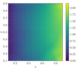
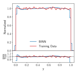
Figure 1: Two-dimensional and marginal densities for the linear wedge ramp.

In Fig. 2 we include the predictive uncertainty given by the BINN. For this purpose we train a network on the two-dimensional parameter space and evaluate it for a set of points with $x\in[0,1]$ and a constant $y$-value. In the left panel we indicate the predictive uncertainty as an error bar around the density estimate. Throughout the paper we always remove the phase space boundaries, because we know that the network is unstable there, and the uncertainties explode just like we expect. For this example, this is taken into account by restricting $x,y\in[0.1,0.9]$. The relative uncertainty grows for small values of $x$ and hence small values of $p(x,y)$, and it covers the deviation of the extracted density from the true density well. These features are common to all our network trainings. In the central and right panel of Fig. 2 we show the relative and absolute predictive uncertainties. The error bar indicates how much $\sigma_{\text{pred}}$ varies for different choices of $y$. We compute it as the standard deviation of different values of $\sigma_{\text{pred}}$, after confirming that the central values agree within this range. As expected, the relative uncertainty decreases towards larger $x$. However, the absolute uncertainty shows a distinctive minimum in $\sigma_{\text{pred}}$ around $x\approx 0.45$. This minimum is a common feature in all our trainings, so we need to explain it.

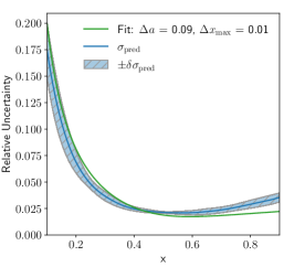
Figure 2: Density and predictive uncertainty distribution for the wedge ramp. In the left panel the density and uncertainty are averaged over several lines with constant $y$. In the central and right panels, the uncertainty band on $\sigma_{\text{pred}}$ is given by their variation. The green curve represents a two-parameter fit to Eq.(23).

To understand this non-trivial uncertainty distribution $\sigma_{\text{pred}}(x)$ we focus on the non-trivial $x$-coordinate and its linear behavior

$$p(x)=ax+b\qquad\text{with}\qquad x\in[0,1]\;.$$ (18)

Because the network learns a density, we can remove $b$ by fixing the normalization,

$$p(x)=a\left(x-\frac{1}{2}\right)+1\;.$$ (19)

If we now assume that a network acts like a fit of $a$, we can relate the uncertainty $\Delta a$ to an uncertainty in the density,

$$\sigma_{\text{pred}}\equiv\Delta p\approx\left|x-\frac{1}{2}\right|\;\Delta a\;.$$ (20)

The absolute value appears because the uncertainties are defined to be positive, as encoded in the usual quadratic error propagation. The uncertainty distribution has a minimum at $x=1/2$, close to the observed value in Fig. 2.

The differences between the simple prediction in Eq.(20) and our numerical findings in Fig. 2 is that the predictive uncertainty is not symmetric and does not reach zero. To account for these sub-leading effects we can expand our very simple ansatz to

$$p(x)=ax+b\qquad\text{with}\qquad x\in[x_{\text{min}},x_{\text{max}}]\;.$$ (21)

Using the normalization condition we again remove $b$ and find

$$p(x)=ax+\frac{1-\frac{a}{2}(x_{\text{max}}^{2}-x_{\text{min}}^{2})}{x_{\text{max}}-x_{\text{min}}}\;.$$ (22)

Again assuming a fit-like behavior of the flow network we expect for the predictive uncertainty

$$\sigma_{\text{pred}}^{2}\equiv(\Delta p)^{2}=\left(x-\frac{1}{2}\right)^{2}(\Delta a)^{2}+\left(1+\frac{a}{2}\right)^{2}(\Delta x_{\text{max}})^{2}+\left(1-\frac{a}{2}\right)^{2}(\Delta x_{\text{min}})^{2}\;.$$ (23)

Adding $x_{\text{min}}$ or $x_{\text{max}}$ leads to an $x$-independent offset and does not change the $x$-dependence of the predictive uncertainty. The slight shift of the minimum and the asymmetry between the lower and upper boundaries in $x$ are not explained by this argument. We ascribe them to boundary effects, specifically the challenge for the network to describe the correct approach towards $p(x)\to 0$.

The green line in Fig. 2 gives a two-parameter fit of $\Delta a$ and $\Delta x_{\text{max}}$ to the $\sigma_{\text{pred}}$ distribution from the BINN. It indicates that there is a hierarchy in the way the network extracts the $x$-independent term with high precision, whereas the uncertainty on the slope $a$ is around 4%.

3.2 Kicker ramp

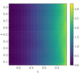
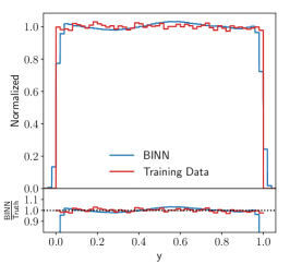
Figure 3: Two-dimensional and marginal densities for the quadratic kicker ramp.

We can test our findings from the linear wedge ramp using the slightly more complex quadratic or kicker ramp,

$$p(x,y)=\text{Quadr}(x\in[0,1])\times\text{Const}(y\in[0,1])=x^{2}\times 3\;.$$ (24)

We show the results from the network training for the density in Fig. 3 and find that the network describes the density well, limited largely by the flat, low-statistics approach towards the lower boundary with $p(x)\to 0$.

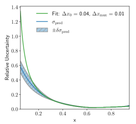
Figure 4: Density and predictive uncertainty distribution for the kicker ramp. In the left panel the density and uncertainty are averaged over several lines with constant $y$. In the central and right panels, the uncertainty band on $\sigma_{\text{pred}}$ is given by their variation. The green curve represents a two-parameter fit to Eq.(27).

In complete analogy to Fig. 2 we show the complete BINN output with the density $p(x,y)$ and the predictive uncertainty $\sigma_{\text{pred}}(x,y)$ in Fig. 4. As for the linear case, the BINN reproduces the density well, deviations from the truth being within the predictive uncertainty in all points of phase space. We remove the phase space boundaries restricting $x,y\in[0.05,0.95]$, as the network becomes unstable and the predictive uncertainties grows correspondingly. The indicated error bar on $\sigma_{\text{pred}}(x,y)$ is given by the variation of the predictions for different $y$-values, after ensuring that their central values agree. The relative uncertainty at the lower boundary $x=0$ is large, reflecting the statistical limitation of this phase space region. An interesting feature appears again in the absolute uncertainty, namely a maximum-minimum combination as a function of $x$.

Again in analogy to Eq.(21) for the wedge ramp, we start with the parametrization of the density

$$p(x)=a\,(x-x_{0})^{2}\qquad\text{with}\qquad x\in[x_{0},x_{\text{max}}]\;,$$ (25)

where we assume that the lower boundary coincides with the minimum and there is no constant offset. We choose to describe this density through the minimum position $x_{0}$, coinciding the the lower end of the $x$-range, and $x_{\text{max}}$ as the second parameter. The parameter $a$ can be eliminated through the normalization condition and we find

$$p(x)=3\frac{(x-x_{0})^{2}}{(x_{\text{max}}-x_{0})^{3}}\;.$$ (26)

If we vary $x_{0}$ and $x_{\text{max}}$ we can trace two contributions to the uncertainty in the density,

$$\sigma_{\text{pred}}\equiv\Delta p \supset\frac{9}{(x_{\text{max}}-x_{0})^{4}}\left|(x-x_{0})\left(x-\frac{x_{0}}{3}-\frac{2x_{\text{max}}}{3}\right)\right|\Delta x_{0}$$

$$\text{and}\qquad\sigma_{\text{pred}}\equiv\Delta p \supset\frac{9}{(x_{\text{max}}-x_{0})^{4}}\;(x-x_{0})^{2}\;\Delta x_{\text{max}}\;,$$ (27)

one from the variation of $x_{0}$ and one from the vriation of $x_{\text{max}}$. In analogy to Eq.(23) they need to be added in quadrature. If the uncertainty on $\Delta x_{0}$ dominates, the uncertainty has a trivial minimum at $x=0$ and a non-trivial minimum at $x=2/3$. From $\Delta x_{\text{max}}$ we get another contribution which scales like $\Delta p\propto p(x)$. In Fig. 4 we clearly observe both contributions, and the green line is given by the corresponding 2-parameter fit to the $\sigma_{\text{pred}}$ distribution from the BINN.

3.3 Gaussian ring

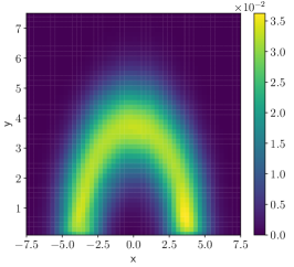
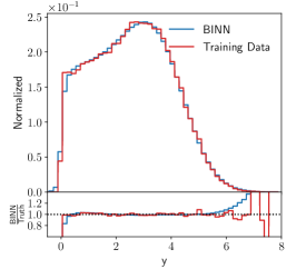
Figure 5: Two-dimensional and marginal densities for the Gaussian (half-)ring.

Our third example is a two dimensional Gaussian ring, which in terms of polar coordinates reads

$$p(r,\phi)=\text{Gauss}(r>0;\mu=4,w=1)\times\text{Const}(\phi\in[0,\pi])\;,$$ (28)

We define the Gaussian density as the usual

$$\text{Gauss}(r) =\frac{1}{\sqrt{2\pi}\;w}\exp\left[-\frac{1}{2w^{2}}(r-\mu)^{2}\right]$$ (29)

The density defined in Eq.(28) can be translated into Cartesian coordinates as

$$p(x,y)=\text{Gauss}(r(x,y);\mu=4,w=1)\,\times\text{Const}(\phi(x,y)\in[0,\pi])\times\dfrac{1}{r(x,y)}$$ (30)

where the additional factor $1/r$ comes from the Jacobian. We train the BINN on Cartesian coordinates, just like in the two examples before, and limit ourselves to $y>0$ to avoid problems induced by learning a non-trivial topology in mapping the latent and phase spaces. In Fig. 5 we once again see that our network describes the true two-dimensional density well.

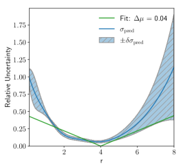
Figure 6: Cartesian density and predictive uncertainty distribution for the Gaussian ring. In the left panel the density and uncertainty are averaged over several lines with constant $\phi$. In the central and right panels, the uncertainty band on $\sigma_{\text{pred}}$ is given by their variation. The green curve represents a two-parameter fit to Eq.(31).

In Fig. 6 we show the Cartesian density but evaluated on a line of constant angle. This form includes the Jacobian and has the expected, slightly shifted peak position at $r_{\text{max}}=2+\sqrt{3}=3.73$. The BINN returns a predictive uncertainty, which grows towards both boundaries. The error band easily covers the deviation of the density learned by the BINN and the true density. While the relative predictive uncertainty appears to have a simple minimum around the peak of the density, we again see that the absolute uncertainty has a distinct structure with a local minimum right at the peak. The question is what we can learn about the INN from this pattern in the BINN.

As before, we describe our distribution in the relevant direction in terms of convenient fit parameters. For the Gaussian radial density these are the mean $\mu$ and the width $w$ used in Eq.(28). The contributions driven by the extraction of the mean in Cartesian coordinates reads

$$\sigma_{\text{pred}} \equiv\Delta p\supset\left|\frac{G(r)}{r}\,\frac{\mu-r}{w^{2}}\right|\Delta\mu$$

$$\text{and}\qquad\sigma_{\text{pred}} \equiv\Delta p\supset\left|\frac{(r-\mu)^{2}}{w^{3}}-\frac{1}{w}\right|\Delta w\;.$$ (31)

In analogy to Eq.(23) the two contributions need to be added in quadrature for the full, fit-like uncertainty. The contribution from the the mean has a minimum at $r=\mu=4$ and is otherwise dominated by the exponential behavior of the Gaussian, just as we observe in the BINN result. In the central and right panels we show a one-parameter fit of the BINN output and find that the network determined the mean of the Gaussian as $\mu=4\pm 0.037$. We observe that including $\Delta w$ doesn’t improve the goodness of the fit.

3.4 Errors vs training statistics

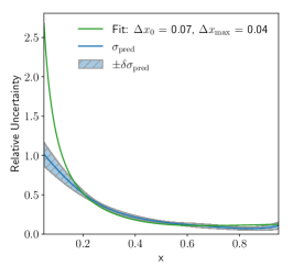
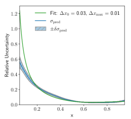
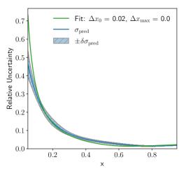
Figure 7: Dependence of the density (upper) and absolute uncertainty (lower) on the training statistics for the kicker ramp. We illustrate BINNs trained on 10k, 100k, and 1M events (left to right), to be compared to 300k events used for Fig. 4. Our training routine ensures that all models receive the same number of weights updates, regardless of the training set size.

Even though it is clear from the above discussion that we cannot expect the predictive uncertainties to have a simple scaling pattern, like for the regression [64] and classification [63] networks, there still remains the question how the BINN uncertainties change with the size of the training sample.

In Fig. 7 we show how the BINN predictions for the density and uncertainty change if we vary the training sample size from 10k events to 1M training events. Note that for all toy models, including the kicker ramp in Sec. 3.2, we use 300k training events. For the small 10k training sample, we see that the instability of the BINN density becomes visible even for our reduced $x$-range. The peak-dip pattern of the absolute uncertainty, characteristic for the kicker ramp, is also hardly visible, indicating that the network has not learned the density well enough to determine its shape. Finally, the variation of the predictive density explodes for $x>0.4$, confirming the picture of a poorly trained BINN. As a rough estimate, the absolute uncertainty at $x=0.5$ with a density value $p(x,y)=0.75$ ranges around $\sigma_{\text{pred}}=0.11~{}...~{}0.15$.

For 100k training events we see that the patterns discussed in Sec. 3.2 begin to form. The density and uncertainty encoded in the network are stable, and the peak-dip with a minimum around $x=2/3$ becomes visible. As a rough estimate we can read off $\sigma_{\text{pred}}(0.5)\approx 0.06\pm 0.03$. For 1M training events the picture improves even more and the network extracts a stable uncertainty of $\sigma_{\text{pred}}(0.5)\approx 0.03\pm 0.01$. Crucially, the dip around $x\approx 2/3$ remains, and even compared to Fig. 4 with its 300k training events the density and uncertainty at the upper phase space boundary are much better controlled.

Finally, we briefly comment on a frequentist interpretation of the BINN output. We know from simpler Bayesian networks [63, 64] that it is possible to reproduce the predictive uncertainty using an ensemble of deterministic networks with the same architecture. However, from those studies we also know that our class of Bayesian networks has a very efficient built-in regularization, so this kind of comparison is not trivial. For the BINN results shown in this paper we find that the detailed patterns in the absolute uncertainties are extracted by the Bayesian network much more efficiently than they would be for ensembles of deterministic INNs. For naive implementations with a similar network size and no fine-tuned regularization these patterns are somewhat harder to extract. On the other hand, in stable regions without distinctive patterns the spread of ensembles of deterministic networks reproduces the predictive uncertainty reported by the BINN.

3.5 Marginalizing phase space

Before we move to a more LHC-related problem, we need to study how the BINN provides uncertainties for marginalized kinematic distribution. In all three toy examples the two-dimensional phase space consists of one physical and one trivial direction. For instance, the kicker ramp in Sec. 3.2 has a quadratic physical direction, and in a typical phase space problem we would integrate out the trivial, constant direction and show a one-dimensional kinematic distribution. From our effectively one-dimensional uncertainty extraction, we know that the absolute uncertainty has a characteristic maximum-minimum combination, as seen in the central panel of Fig. 4.

To compute the uncertainty for a properly marginalized phase space direction, we remind ourselves how the BINN computes the density and the predictive uncertainty by sampling over the weights,

$$p(x,y) =\int d\theta\,q(\theta)\,p(x,y|\theta)$$

$$\sigma_{\text{pred}}^{2}(x,y) =\int d\theta\,q(\theta)\left[p(x,y|\theta)-p(x,y)\right]^{2}\,.$$ (32)

If we integrate over the $y$-direction, the marginalized density is defined as

$$p(x)=\int dy\,p(x,y)= \int dyd\theta\,q(\theta)\,p(x,y|\theta)$$

$$= \int d\theta\,q(\theta)\,\int dy\,p(x,y|\theta)\equiv\int d\theta\,q(\theta)\,p(x|\theta)\;,$$ (33)

which implicitly defines $p(x|\theta)$ in the last step, notably without providing us with a way to extract it in a closed form. The key step in this definition is that we exchange the order of the $y$ and $\theta$ integrations. Nevertheless, with this definition at hand, we can define the uncertainty on the marginalized distribution as

$$\sigma_{\text{pred}}^{2}(x)=\int d\theta\,q(\theta)\left[p(x|\theta)-p(x)\right]^{2}\;.$$ (34)

We illustrate this construction with a trivial $p(x,y)=p(x,y_{0})$, where we can replace the trivial $y$-dependence by a fixed choice $y=y_{0}$ just like for the wedge and kicker ramps. Here we find, modulo a normalization constant in the $y$-integration

$$\sigma_{\text{pred}}^{2}(x) =\int d\theta\,q(\theta)\left[p(x|\theta)-p(x)\right]^{2}$$

$$=\int d\theta\,q(\theta)\int dy\;\left[p(x,y_{0}|\theta)-p(x,y_{0})\right]^{2}$$

$$=\int dyd\theta\,q(\theta)\;\left[p(x,y_{0}|\theta)-p(x,y_{0})\right]^{2}=\int dy\,\sigma_{\text{pred}}^{2}(x,y_{0})=\sigma_{\text{pred}}^{2}(x,y_{0})\;.$$ (35)

Adding a trivial $y$-direction does not affect the predictive uncertainty in the physical $x$-direction.

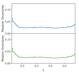
Figure 8: Marginalized densities and predictive uncertainties for the kicker ramp. Instead of the true distribution we now show the training data as a reference, to illustrate possible limitations. We use 10M phase space point to guarantee a stable prediction.

As mentioned above, unlike for the joint density $p(x,y|\theta)$, we do not know the closed form of the marginal distributions $p(x)$ or $p(x|\theta)$. Instead, we can approximate the marginalized uncertainties through a combined sampling in $y$ and $\theta$. We start with one set of weights $\theta_{i}$ from the weight distribution, based on one random number per INN weight. We now sample $N$ points in the latent space, $z_{j}$, and compute $N$ phase space points $x_{j}$ using the BINN configuration $\theta_{i}$. We then bin the wanted phase space direction $x$ and approximate $p(x|\theta_{i})$ by a histogram. We repeat this procedure $i=1~{}...~{}M$ times to extract $M$ histograms with identical binning. This allows us to compute a mean and a standard deviation from $M$ histograms to approximate $p(x)$ and $\sigma_{\text{pred}}(x)$. The approximation of $\sigma_{\text{pred}}$ should be an over-estimate, because it includes the statistical uncertainty related to a finite number of samples per bin. For $N\gg 1$ this contribution should become negligible. With this procedure we effectively sample $N\times M$ points in phase space.

Following Eq.(33), we can also fix the phase space points, so instead of sampling for each weight sample another set of phase space points, we use the same phase space points for each weight sampling. This should stabilize the statistical fluctuations, but with the drawback of relying only on an effective number of $N$ phase space points. Both approaches lead to the same $\sigma_{\text{pred}}$ for sufficiently large $N$, which we typically set to $10^{5}~{}...~{}10^{6}$. For the Bayesian weights we find stable results for $M=30~{}...~{}50$.

In Fig. 8 we show the marginalized densities and predictive uncertainties for the kicker ramp. In $y$-direction the density and the predictive uncertainty show the expected flat behavior. The only exceptions are the phase space boundaries, where the density starts to deviate slightly from the training data and the uncertainty correctly reflects that instability. In $x$-direction, the marginalized density and uncertainty can be compared to their one-dimensional counterparts in Fig.4. While we expect the same peak-dip structure, the key question is if the numerical values for $\sigma_{\text{pred}}(x)$ change. If the network learns the $y$-direction as uncorrelated additional data, the marginalized uncertainty should decrease through a larger effective training sample. This is what we typically see for Monte Carlo simulations, where a combination of bins in an unobserved direction leads to the usual reduced statistical uncertainty. On the other hand, if the network learns that the $y$-directions is flat, then adding events in this direction will have no effect on the uncertainty of the marginalized distribution. This would correspond to a set of fully correlated bins, where a combination will not lead to any improvement in the uncertainty. In Fig. 8 we see that the $\sigma_{\text{pred}}(x)$ values on the peak, in the dip, and to the upper end of the phase space boundary hardly change from the one-dimensional results in Fig.4. This confirms our general observation, that the (B)INN learns a functional form of the density in both directions, in close analogy to a fit. It also means that the uncertainty from the generative network training is not described by the simple statistical scaling we observed for simpler networks [63, 64] and instead points towards a GANplification-like [4] pattern.

4 LHC events with uncertainties

Parameter	Flow
Hidden layers (per block)	2
Units per hidden layer	64
Batch size	512
Epochs	500
Trainable weights	$\sim$ 182k
Number of training events	$\sim$ 1M
Optimizer	Adam
($\alpha$, $\beta_{1}$, $\beta_{2}$)	($1\times 10^{-3}$, 0.9, 0.999)
Coupling layers	20
Prior width	1

Table 2: Hyper-parameters for the Drell-Yan data set, implemented in PyTorch (v1.4.0) [75].

As a physics example we consider the Drell-Yan process

$$pp\rightarrow Z\rightarrow e^{+}e^{-}\;,$$ (36)

with its simple $2\to 2$ phase space combined with the parton density. The training set consists of an unweighted set of 4-vectors simulated with Madgraph5 [76] at 13 TeV collider energy with the NNPDF2.3 parton densities [77]. We fix the masses of the final-state leptons and enforce momentum conservation in the transverse direction, which leaves us with a four-dimensional phase space. In our discussion we limit ourselves to a sufficiently large set of one-dimensional distributions. For these marginalized uncertainties we follow the procedure laid out in Sec. 3.5 with 50 samples in the BINN-weight space. In Tab. 2 we give the relevant hyper-parameters for this section.

Figure 9: One-dimensional (marginalized) kinematic distributions for the Drell-Yan process. We show the central prediction from the BINN and include the predictive uncertainty from the BINN as the blue band. The red band indicates the statistical uncertainty of the training data per bin in the Gaussian limit.

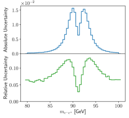
Figure 10: Absolute and relative uncertainties as a function of some of the kinematic Drell-Yan observables shown in Fig. 9.

To start with, we show a set of generated kinematic distributions in Fig. 9. The positron energy features the expected strong peak from the $Z$-resonance. Its sizeable tail to larger energies is well described by the training data to $E_{e}\approx 280$ GeV. The central value learned by the BINN becomes unstable at slightly lower values of 250 GeV, as expected. The momentum component $p_{x}$ is not observable given the azimuthal symmetry of the detector, but it’s broad distribution is nevertheless reproduced correctly. The predictive uncertainty covers the slight deviations over the entire range. What is observable at the LHC is the transverse momentum of the outgoing leptons, with a similar distribution as the energy, just with the $Z$-mass peak at the upper end of the distribution. Again, the predictive uncertainty determined by the BINN covers the slight deviations from the truth on the pole and in both tails. In the second row we show the $p_{z}$ component as an example of a strongly peaked distribution, similar to the Gaussian toy model in Sec. 3.3.

While the energy of the lepton pair has a similar basic form as the individual energies, we also show the invariant mass of the electron-positron pair, which is described by the usual Breit-Wigner peak. It is well known that this intermediate resonance is especially hard to learn for a network, because it forms a narrow, highly correlated phase space structure. Going beyond the precision shown here would for instance require an additional MMD loss, as described in Ref. [25] and in more detail in Ref. [54]. This resonance peak is the only distribution where the predictive uncertainty does not cover the deviation of the BINN density from the truth. This apparent failure corresponds to the fact that generative networks always overestimate the width and hence underestimate the height of this mass peak [25]. This is an example of the network being limited by the expressive power in phase space resolution, generating an uncertainty which the Bayesian version cannot account for.

In Fig. 10 we show a set of absolute and relative uncertainties from the BINN. The strong peak combined with a narrow tail in the $E_{e}$ distribution shows two interesting features. Just above the peak the absolute uncertainty drops more rapidly than expected, a feature shared by the wedge and kicker ramps at their respective upper phase space boundaries. The shoulder around $E_{e}\approx 280$ GeV indicates that for a while the predictive uncertainty follows the increasingly poor modelling of the phase space density by the BINN, to a point where the network stops following the truth curve altogether and the predictive uncertainty is limited by the expressive power of the network. Unlike the absolute uncertainty, the relative uncertainty keeps growing for increasing values of $E_{e}$. This behavior illustrates that in phase space regions where the BINN starts failing altogether, we cannot trust the predictive uncertainty either, but we see a pattern in the intermediate phase space regime where the network starts failing.

The second kinematic quantity we select is the (unobservable) $x$-component of the momentum. It forms a relative flat central plateau with sharp cliffs at each side. Any network will have trouble learning the exact shape of such sharp phase space patterns. Here the BINN keeps track of this, the absolute and the relative predictive uncertainties indeed explode. The only difference between the two is that the (learned) density at the foot of the plateau drops even faster than the learned absolute uncertainty, so their ratio keeps growing.

Finally, we show the result for the Breit-Wigner mass peak, the physical counterpart of the Gaussian ring model of Sec. 3.3. Indeed, we see exactly the same pattern, namely a distinctive minimum in the predictive uncertainty right on the mass peak. This pattern can be explained by the network learning the general form of a mass peak and then adjusting the mean and the width of this peak. Learning the peak position leads to a minimum of the uncertainty right at the peak, and learning the width brings up two maxima on the shoulders of the mass peak. In combination Fig. 9 and 10 clearly show that the BINN traces uncertainties in generated LHC events just as for the toy models. Again, some distinctive patterns in the predictive uncertainty can be explained by the way the network learns the phase space density.

5 Outlook

Controlling the output of generative networks and quantifying their uncertainties is the main task for any application in LHC physics, be it in forward generation, inversion, or inference. We have proposed to use a Bayesian invertible network (BINN) to quantify the uncertainties from the network training for each generated event. For a series of two-dimensional toy models and an LHC-inspired application we have shown how the Bayesian setup indeed generates an uncertainty distribution, over the full phase space and over marginalized phase spaces. As expected, the learned uncertainty shrinks with an improved training statistics. Our method can be trivially extended from unweighted to weighted events by adapting the simple MLE loss.

An intriguing result from our study is that the combined learning of the density and uncertainty distributions allows us to draw conclusions on how a normalizing-flow network like the BINN learns a distribution. We find that the uncertainty distributions are naturally explained by a fit-like behavior of the network, rather than a patch-wise learning of the density. For the LHC, this can be seen for instance in the non-trivial uncertainty for an intermediate Breit-Wigner resonance. These results are another step in understanding GANplification patterns [4] and might even allow us to use INNs to extrapolate in phase space.

Obviously, it remains to be seen how our observations generalize to other generative networks architectures. For the LHC, the next step should be an in-depth study of INN-like networks applied to event generation.

Acknowledgments

We are very grateful for many discussions with Lynton Ardizzone, Anja Butter, Gregor Kasieczka, Ullrich Köthe, and Ramon Winterhalder. The research of TP is supported by the Deutsche Forschungsgemeinschaft (DFG, German Research Foundation) under grant 396021762 – TRR 257 Particle Physics Phenomenology after the Higgs Discovery. MB is supported by the International Max Planck School Precision Tests of Fundamental Symmetries. ML is supported by the DFG Research Training Group GK-1940, Particle Physics Beyond the Standard Model.

References

- [1] A. Butter and T. Plehn, Generative Networks for LHC events, arXiv:2008.08558 [hep-ph].
- [2] I. J. Goodfellow, J. Pouget-Abadie, M. Mirza, B. Xu, D. Warde-Farley, S. Ozair, A. Courville, and Y. Bengio, Generative adversarial networks, arXiv:1406.2661 [stat.ML].
- [3] A. Creswell, T. White, V. Dumoulin, K. Arulkumaran, B. Sengupta, and A. A. Bharath, Generative adversarial networks: An overview, IEEE Signal Processing Magazine 35 (Jan, 2018) 53–65.
- [4] A. Butter, S. Diefenbacher, G. Kasieczka, B. Nachman, and T. Plehn, GANplifying Event Samples, arXiv:2008.06545 [hep-ph].
- [5] D. P. Kingma and M. Welling, Auto-encoding variational bayes, arXiv:1312.6114 [stat.ML].
- [6] D. P. Kingma and M. Welling, An introduction to variational autoencoders, Foundations and Trends® in Machine Learning 12 (2019) 4, 307–392.
- [7] D. Rezende and S. Mohamed, Variational inference with normalizing flows, in Proceedings of the 32nd International Conference on Machine Learning, F. Bach and D. Blei, eds. PMLR, Lille, France, 07–09 Jul, 2015. arXiv:1505.05770 [stat.ML].
- [8] I. Kobyzev, S. Prince, and M. Brubaker, Normalizing flows: An introduction and review of current methods, IEEE Transactions on Pattern Analysis and Machine Intelligence (2020) 1–1.
- [9] G. Papamakarios, E. Nalisnick, D. J. Rezende, S. Mohamed, and B. Lakshminarayanan, Normalizing flows for probabilistic modeling and inference, arXiv:1912.02762 [stat.ML].
- [10] I. Kobyzev, S. Prince, and M. A. Brubaker, Normalizing flows: An introduction and review of current methods, arXiv:1908.09257 [stat.ML].
- [11] T. Müller, B. McWilliams, F. Rousselle, M. Gross, and J. Novák, Neural importance sampling, arXiv:1808.03856 [cs.LG].
- [12] L. Ardizzone, J. Kruse, S. Wirkert, D. Rahner, E. W. Pellegrini, R. S. Klessen, L. Maier-Hein, C. Rother, and U. Köthe, Analyzing inverse problems with invertible neural networks, arXiv:1808.04730 [cs.LG].
- [13] L. Dinh, J. Sohl-Dickstein, and S. Bengio, Density estimation using real nvp, arXiv:1605.08803 [cs.LG].
- [14] D. P. Kingma and P. Dhariwal, Glow: Generative flow with invertible 1x1 convolutions, arXiv:1807.03039 [stat.ML].
- [15] M. D. Klimek and M. Perelstein, Neural Network-Based Approach to Phase Space Integration, arXiv:1810.11509 [hep-ph].
- [16] I.-K. Chen, M. D. Klimek, and M. Perelstein, Improved Neural Network Monte Carlo Simulation, SciPost Phys. 10 (2021) 023, arXiv:2009.07819 [hep-ph].
- [17] E. Bothmann, T. Janßen, M. Knobbe, T. Schmale, and S. Schumann, Exploring phase space with Neural Importance Sampling, SciPost Phys. 8 (2020) 4, 069, arXiv:2001.05478 [hep-ph].
- [18] C. Gao, J. Isaacson, and C. Krause, i-flow: High-dimensional Integration and Sampling with Normalizing Flows, arXiv:2001.05486 [physics.comp-ph].
- [19] C. Gao, S. Höche, J. Isaacson, C. Krause, and H. Schulz, Event Generation with Normalizing Flows, Phys. Rev. D 101 (2020) 7, 076002, arXiv:2001.10028 [hep-ph].
- [20] F. Bishara and M. Montull, (Machine) Learning Amplitudes for Faster Event Generation, arXiv:1912.11055 [hep-ph].
- [21] S. Badger and J. Bullock, Using neural networks for efficient evaluation of high multiplicity scattering amplitudes, arXiv:2002.07516 [hep-ph].
- [22] S. Otten et al., Event Generation and Statistical Sampling with Deep Generative Models and a Density Information Buffer, arXiv:1901.00875 [hep-ph].
- [23] B. Hashemi, N. Amin, K. Datta, D. Olivito, and M. Pierini, LHC analysis-specific datasets with Generative Adversarial Networks, arXiv:1901.05282 [hep-ex].
- [24] R. Di Sipio, M. Faucci Giannelli, S. Ketabchi Haghighat, and S. Palazzo, DijetGAN: A Generative-Adversarial Network Approach for the Simulation of QCD Dijet Events at the LHC, JHEP 08 (2020) 110, arXiv:1903.02433 [hep-ex].
- [25] A. Butter, T. Plehn, and R. Winterhalder, How to GAN LHC Events, SciPost Phys. 7 (2019) 075, arXiv:1907.03764 [hep-ph].
- [26] Y. Alanazi, N. Sato, T. Liu, W. Melnitchouk, M. P. Kuchera, E. Pritchard, M. Robertson, R. Strauss, L. Velasco, and Y. Li, Simulation of electron-proton scattering events by a Feature-Augmented and Transformed Generative Adversarial Network (FAT-GAN), arXiv:2001.11103 [hep-ph].
- [27] A. Butter, T. Plehn, and R. Winterhalder, How to GAN Event Subtraction, SciPost Phys. Core 3 (2020) 009, arXiv:1912.08824 [hep-ph].
- [28] B. Stienen and R. Verheyen, Phase Space Sampling and Inference from Weighted Events with Autoregressive Flows, SciPost Phys. 10 (2021) 038, arXiv:2011.13445 [hep-ph].
- [29] M. Backes, A. Butter, T. Plehn, and R. Winterhalder, How to GAN Event Unweighting, arXiv:2012.07873 [hep-ph].
- [30] M. Paganini, L. de Oliveira, and B. Nachman, Accelerating Science with Generative Adversarial Networks: An Application to 3D Particle Showers in Multilayer Calorimeters, Phys. Rev. Lett. 120 (2018) 4, 042003, arXiv:1705.02355 [hep-ex].
- [31] M. Paganini, L. de Oliveira, and B. Nachman, CaloGAN : Simulating 3D high energy particle showers in multilayer electromagnetic calorimeters with generative adversarial networks, Phys. Rev. D97 (2018) 1, 014021, arXiv:1712.10321 [hep-ex].
- [32] P. Musella and F. Pandolfi, Fast and Accurate Simulation of Particle Detectors Using Generative Adversarial Networks, Comput. Softw. Big Sci. 2 (2018) 1, 8, arXiv:1805.00850 [hep-ex].
- [33] M. Erdmann, L. Geiger, J. Glombitza, and D. Schmidt, Generating and refining particle detector simulations using the Wasserstein distance in adversarial networks, Comput. Softw. Big Sci. 2 (2018) 1, 4, arXiv:1802.03325 [astro-ph.IM].
- [34] M. Erdmann, J. Glombitza, and T. Quast, Precise simulation of electromagnetic calorimeter showers using a Wasserstein Generative Adversarial Network, Comput. Softw. Big Sci. 3 (2019) 4, arXiv:1807.01954 [physics.ins-det].
- [35] ATLAS Collaboration, “Deep generative models for fast shower simulation in ATLAS.” ATL-SOFT-PUB-2018-001, 2018. http://cds.cern.ch/record/2630433.
- [36] ATLAS Collaboration, “Energy resolution with a GAN for Fast Shower Simulation in ATLAS.” ATLAS-SIM-2019-004, 2019. https://atlas.web.cern.ch/Atlas/GROUPS/PHYSICS/PLOTS/SIM-2019-004/.
- [37] D. Belayneh et al., Calorimetry with Deep Learning: Particle Simulation and Reconstruction for Collider Physics, Eur. Phys. J. C 80 (2020) 7, 688, arXiv:1912.06794 [physics.ins-det].
- [38] E. Buhmann, S. Diefenbacher, E. Eren, F. Gaede, G. Kasieczka, A. Korol, and K. Krüger, Getting High: High Fidelity Simulation of High Granularity Calorimeters with High Speed, arXiv:2005.05334 [physics.ins-det].
- [39] E. Buhmann, S. Diefenbacher, E. Eren, F. Gaede, G. Kasieczka, A. Korol, and K. Krüger, Decoding Photons: Physics in the Latent Space of a BIB-AE Generative Network, arXiv:2102.12491 [physics.ins-det].
- [40] E. Bothmann and L. Debbio, Reweighting a parton shower using a neural network: the final-state case, JHEP 01 (2019) 033, arXiv:1808.07802 [hep-ph].
- [41] L. de Oliveira, M. Paganini, and B. Nachman, Learning Particle Physics by Example: Location-Aware Generative Adversarial Networks for Physics Synthesis, Comput. Softw. Big Sci. 1 (2017) 1, 4, arXiv:1701.05927 [stat.ML].
- [42] J. W. Monk, Deep Learning as a Parton Shower, JHEP 12 (2018) 021, arXiv:1807.03685 [hep-ph].
- [43] A. Andreassen, I. Feige, C. Frye, and M. D. Schwartz, JUNIPR: a Framework for Unsupervised Machine Learning in Particle Physics, Eur. Phys. J. C79 (2019) 2, 102, arXiv:1804.09720 [hep-ph].
- [44] K. Dohi, Variational Autoencoders for Jet Simulation, arXiv:2009.04842 [hep-ph].
- [45] J. Lin, W. Bhimji, and B. Nachman, Machine Learning Templates for QCD Factorization in the Search for Physics Beyond the Standard Model, JHEP 05 (2019) 181, arXiv:1903.02556 [hep-ph].
- [46] B. Nachman and D. Shih, Anomaly Detection with Density Estimation, Phys. Rev. D 101 (2020) 075042, arXiv:2001.04990 [hep-ph].
- [47] O. Knapp, G. Dissertori, O. Cerri, T. Q. Nguyen, J.-R. Vlimant, and M. Pierini, Adversarially Learned Anomaly Detection on CMS Open Data: re-discovering the top quark, arXiv:2005.01598 [hep-ex].
- [48] F. A. Di Bello, S. Ganguly, E. Gross, M. Kado, M. Pitt, L. Santi, and J. Shlomi, Towards a Computer Vision Particle Flow, Eur. Phys. J. C 81 (2021) 2, 107, arXiv:2003.08863 [physics.data-an].
- [49] P. Baldi, L. Blecher, A. Butter, J. Collado, J. N. Howard, F. Keilbach, T. Plehn, G. Kasieczka, and D. Whiteson, How to GAN Higher Jet Resolution, arXiv:2012.11944 [hep-ph].
- [50] J. Brehmer and K. Cranmer, Flows for simultaneous manifold learning and density estimation, arXiv:2003.13913 [stat.ML].
- [51] S. T. Radev, U. K. Mertens, A. Voss, L. Ardizzone, and U. Köthe, Bayesflow: Learning complex stochastic models with invertible neural networks, arXiv:2003.06281 [stat.ML].
- [52] S. Bieringer, A. Butter, T. Heimel, S. Höche, U. Köthe, T. Plehn, and S. T. Radev, Measuring QCD Splittings with Invertible Networks, arXiv:2012.09873 [hep-ph].
- [53] K. Datta, D. Kar, and D. Roy, Unfolding with Generative Adversarial Networks, arXiv:1806.00433 [physics.data-an].
- [54] M. Bellagente, A. Butter, G. Kasieczka, T. Plehn, and R. Winterhalder, How to GAN away Detector Effects, SciPost Phys. 8 (2020) 4, 070, arXiv:1912.00477 [hep-ph].
- [55] M. Bellagente, A. Butter, G. Kasieczka, T. Plehn, A. Rousselot, R. Winterhalder, L. Ardizzone, and U. Köthe, Invertible Networks or Partons to Detector and Back Again, SciPost Phys. 9 (2020) 074, arXiv:2006.06685 [hep-ph].
- [56] D. MacKay, Probable Networks and Plausible Predictions – A Review of Practical Bayesian Methods for Supervised Neural Networks, Comp. in Neural Systems 6 (1995) 4679.
- [57] R. M. Neal, Bayesian learning for neural networks. PhD thesis, Toronto, 1995.
- [58] Y. Gal, Uncertainty in Deep Learning. PhD thesis, Cambridge, 2016.
- [59] A. Kendall and Y. Gal, What Uncertainties Do We Need in Bayesian Deep Learning for Computer Vision?, Proc. NIPS (2017) , arXiv:1703.04977 [cs.CV].
- [60] P. C. Bhat and H. B. Prosper, Bayesian neural networks, Conf. Proc. C 050912 (2005) 151.
- [61] S. R. Saucedo, Bayesian Neural Networks for Classification, Master’s thesis, Florida State University, 2007.
- [62] Y. Xu, W. Xu, Y. Meng, K. Zhu, and W. Xu, Applying Bayesian Neural Networks to Event Reconstruction in Reactor Neutrino Experiments, Nucl. Instrum. Meth. A 592 (2008) 451, arXiv:0712.4042 [physics.data-an].
- [63] S. Bollweg, M. Haußmann, G. Kasieczka, M. Luchmann, T. Plehn, and J. Thompson, Deep-Learning Jets with Uncertainties and More, SciPost Phys. 8 (2020) 1, 006, arXiv:1904.10004 [hep-ph].
- [64] G. Kasieczka, M. Luchmann, F. Otterpohl, and T. Plehn, Per-Object Systematics using Deep-Learned Calibration, SciPost Phys. 9 (2020) 089, arXiv:2003.11099 [hep-ph].
- [65] B. Nachman, A guide for deploying Deep Learning in LHC searches: How to achieve optimality and account for uncertainty, SciPost Phys. 8 (2020) 090, arXiv:1909.03081 [hep-ph].
- [66] J. Y. Araz and M. Spannowsky, Combine and Conquer: Event Reconstruction with Bayesian Ensemble Neural Networks, arXiv:2102.01078 [hep-ph].
- [67] D. J. MacKay, Probable networks and plausible predictions—a review of practical bayesian methods for supervised neural networks, Network: computation in neural systems 6 (1995) 3, 469.
- [68] R. M. Neal, Bayesian learning for neural networks, vol. 118. Springer Science & Business Media, 2012.
- [69] C. Louizos, M. Welling, and D. P. Kingma, Learning sparse neural networks through l_0 regularization, in International Conference on Learning Representations. 2018. arXiv:1712.01312 [stat.ML].
- [70] S. Ghosh, J. Yao, and F. Doshi-Velez, Structured variational learning of bayesian neural networks with horseshoe priors, in International Conference on Machine Learning, PMLR. 2018. arXiv:1806.05975 [cs.LG].
- [71] J. T. Springenberg, A. Klein, S. Falkner, and F. Hutter, Bayesian optimization with robust bayesian neural networks, in Advances in Neural Information Processing Systems, D. Lee, M. Sugiyama, U. Luxburg, I. Guyon, and R. Garnett, eds. Curran Associates, Inc., 2016.
- [72] D. M. Blei, A. Kucukelbir, and J. D. McAuliffe, Variational inference: A review for statisticians, Journal of the American statistical Association 112 (2017) 518, 859.
- [73] D. P. Kingma and J. Ba, Adam: A method for stochastic optimization, in 3rd International Conference on Learning Representations, ICLR 2015, San Diego, CA, USA, May 7-9, 2015, Conference Track Proceedings, Y. Bengio and Y. LeCun, eds. 2015.
- [74] D. P. Kingma, T. Salimans, and M. Welling, Variational dropout and the local reparameterization trick, in Advances in neural information processing systems. 2015.
- [75] A. Paszke, S. Gross, F. Massa, A. Lerer, J. Bradbury, G. Chanan, T. Killeen, Z. Lin, N. Gimelshein, L. Antiga, A. Desmaison, A. Kopf, E. Yang, Z. DeVito, M. Raison, A. Tejani, S. Chilamkurthy, B. Steiner, L. Fang, J. Bai, and S. Chintala, Pytorch: An imperative style, high-performance deep learning library, in Advances in Neural Information Processing Systems 32, H. Wallach, H. Larochelle, A. Beygelzimer, F. d’Alché Buc, E. Fox, and R. Garnett, eds., pp. 8024–8035. Curran Associates, Inc., 2019. arXiv:1912.01703 [cs.LG].
- [76] J. Alwall et al., The automated computation of tree-level and next-to-leading order differential cross sections, and their matching to parton shower simulations, JHEP 07 (2014) 079, arXiv:1405.0301 [hep-ph].
- [77] NNPDF, R. D. Ball, V. Bertone, S. Carrazza, L. Del Debbio, S. Forte, A. Guffanti, N. P. Hartland, and J. Rojo, Parton distributions with QED corrections, Nucl. Phys. B877 (2013) 290, arXiv:1308.0598 [hep-ph].