Compressing PDF sets using generative adversarial networks

Abstract

We present a compression algorithm for parton densities using synthetic replicas generated from the training of a Generative Adversarial Network (GAN). The generated replicas are used to further enhance the statistics of a given Monte Carlo PDF set prior to compression. This results in a compression methodology that is able to provide a compressed set with smaller number of replicas and a more adequate representation of the original probability distribution. We also address the question of whether the GAN could be used as an alternative mechanism to avoid the fitting of large number of replicas.

1 Introduction

Parton distribution functions (PDFs) are crucial ingredients for all predictions of physical observables at hadron colliders such as the LHC, and efforts to push their uncertainties to smaller values are becoming increasingly relevant. As a matter of fact, they are one of the dominant sources of uncertainties in precision measurements. An example of this is the limitation that PDFs play in the extraction of the Higgs couplings from data Cepeda:2019klc .

In the past few years, several methods have been developed to make the determination of PDFs more precise. To date, there exists various PDF fitter groups Ball:2017nwa ; Bailey:2020ooq ; Hou:2019jgw ; Alekhin:2013nda implementing different methodologies and providing PDF sets with different estimates of the associated uncertainties. In the NNPDF approach, where the PDFs are represented in terms of an ensemble of Monte Carlo replicas Ball:2017nwa , a large number of those replicas are required in order to reproduce the most accurate representation of the underlying probability distribution. There has been considerable evidence Carrazza:2015hva ; Badger:2016bpw ; Butterworth:2015oua that the convergence of the Monte Carlo PDF replicas to the asymptotic result is slow, and one might require $\mathcal{O}(1000)$ replicas to get accurate results. As a matter of fact, one of the main differences between a fit with $100$ and $1000$ Monte Carlo replicas is that correlations between PDFs are reproduced more accurately in the latter Carrazza:2015hva . From a practical point of view, however, there are challenges related to the use of such a large set of PDF members. Indeed, having to deal with a large ensemble of replicas when producing phenomenological studies is not ideal. To address this issue, a compression methodology that reduces the original Monte Carlo PDF set into a smaller subset was introduced in Ref. Carrazza:2015hva . Conceptually, the compression works by searching for the subset of replicas that reproduces best the statistical features of the original prior PDF distribution.

In this paper, we propose a new compression strategy that aims to provide a compressed set with an even smaller number of replicas when compared to Ref. Carrazza:2015hva , while maintaining an accurate representation of the original probability distribution. Our approach relies on the deep learning techniques usually known as Generative Adversarial Neural Networks NIPS2014_5ca3e9b1 or GANs in short. GANs belong to the class of unsupervised machine learning algorithms where a generative model is trained to produce new data which is indistinguishable under certain criteria from the training data. GANs are mainly used for image modeling zhu2020unpaired , but in the last couple years, many applications have been found in High Energy Physics (HEP) deOliveira:2017pjk ; Paganini:2017dwg ; Butter:2019eyo ; Bellagente:2019uyp ; Butter:2019cae ; Carrazza:2019cnt ; Backes:2020vka ; Butter:2020tvl ; Butter:2020qhk ; Matchev:2020tbw . Here, we propose to use the GANs to enhance the statistics of a given input Monte Carlo PDF by generating what we call synthetic replicas. This is supported by the following observation: large replica samples contain fluctuations that average out to the asymptotic limit. In the standard approach, the job of the PDF compressor is to only extract samples that present small fluctuations and which reproduce best the statistical properties of the original distribution. It should be therefore possible to use GANs to generate samples of replicas that contain less fluctuations and once combined with samples from the prior lead to a more efficient compressed representation of the full result.

Despite the fact that the techniques described in this paper might be generalizable to produce larger PDF sets, we emphasize that our main goal is to provide a technique for minimizing the information loss due to the compression of larger into smaller sets.

The paper is organized as follows. Section 2 and 3 provide a brief description of the compression and GAN methodologies respectively. The framework in which the two methodologies are combined together is described in Section 4. Section 5 presents the results, highlighting the improvement with respect to the previous compression methodology. Section 6 gives an outlook of the potential usage of GANs to by-pass the fitting procedure.

2 Compression: methodological review

Let us begin by giving a brief review of the compression methodology formally introduced in Ref. Carrazza:2015hva . The underlying idea behind the compression of (combined) Monte Carlo PDF replicas consists in finding a subset of the original set of PDF replicas such that the statistical distance between the original and compressed probability distributions is minimal.

The compression strategy relies on two main ingredients: first, a proper definition of the distance metric that measure the difference between the prior and the compressed distributions; second, an appropriate minimization algorithm that explores the space of minima.

As originally proposed Carrazza:2015hva , a suitable figure of merit to quantify the distinguishability between the prior and compressed probability distributions is the error function:

$$\mathrm{ERF}=\frac{1}{N_{\text{EST}}}\sum_{k}\frac{1}{N_{k}}\sum_{i}\left(\frac{C^{k}(x_{i})-P^{k}(x_{i})}{P^{k}(x_{i})}\right)^{2},$$ (1)

where $N_{\text{EST}}$ denotes the total number of statistical estimators used to quantify the distance between the prior and compressed PDF sets, $k$ runs over all statistical estimators with $N_{k}$ the appropriate normalization factor, $P^{k}(x_{i})$ is the value of the estimator $k$ computed at a given point $i$ in the $x$ grid, and $C^{k}(x_{i})$ is the corresponding value of the same estimator for the compressed distribution. The scale at which the PDFs are computed is fixed and the same for all estimators. The list of statistical estimators entering the expression of the total error function in Eq. 1 includes lower moments (such as mean and standard deviation) and standardized moments (such as Skewness and Kurtosis). In addition, in order to preserve higher moments and PDF-induced correlations in physical cross sections, the Kolmogorov-Smirnov and the correlation between multiple PDF flavours are also considered. For each estimator, a proper normalization factor has to be included in order to compensate for the various orders of magnitude in different regions in the $(x,Q)$ space mainly present in higher moments. For an ample description of the individual statistical estimators with the respective expression of their normalization factors, we refer the reader to the original compression paper Carrazza:2015hva .

Once the set of statistical estimators and the target size of the compressed PDF set are defined, the compression algorithm searches for the combination of replicas that leads to the minimal value of the total error function. Due to the discrete nature of the compression problem, it is adequate to perform the minimization using Evolution Algorithm (EA) strategies such as the Genetic Algorithm (GA) or the Covariance Matrix Adaptation (CMA) to select the replicas entering the compressed set.

The methodology presented above is currently implemented in a C++ code referred to as compressor Carrazza:2015hva which uses a GA as the minimization strategy. In order to construct a new framework that allows for various methodological enhancements, we have developed a new compression code written in python and based on the object oriented approach for grater flexibility and maintainability. Henceforth, we refer to the new implementation as pyCompressor Compressor:2020 . The new framework provides additional features such as the Covariance Matrix Adaptative (CMA) minimization strategy and the adiabatic minimization procedure, whose relevance will be explained in the next sections. In addition to the above-mentioned advantages, the new code is also faster. A benchmark comparison with the compressor is presented in App. A.

By default, the pyCompressor computes the input PDF grid for $n_{f}=8$ light partons $(g,u,s,d,c,\bar{u},\bar{s},\bar{d})$ at some energy scale (ex: $Q_{0}=$1.65\text{\,}\mathrm{GeV}$$). The range of $x$ points is restricted within the regions where experimental data are available, namely $(10^{-5},1)$. The default estimators are the same as the ones considered in Ref. Carrazza:2015hva .

3 How to GAN PDFs?

The following section describes how techniques from generative adversarial models could be used to improve the efficiency of the compression algorithm. The framework presented here has been implemented in a standalone python package that we dubbed ganpdfs ganpdfs:2020 . The idea is to use generative neural networks to enhance the statistics of the original Monte Carlo PDF replicas prior to the compression by generating synthetic PDF replicas.

3.1 Introduction to GANs for PDFs

The problem we are concerned with is the following: suppose our Monte Carlo PDF replicas follow a probability distribution $p_{R}$, we would like to generate synthetic replicas following some probability distribution $p_{\theta}$ such that $p_{\theta}$ is very close to $p_{R}$, i.e, the Kullback-Leibler divergence

$$\mathrm{KL}\left(p_{R}||p_{\theta}\right)=\int_{x}\mathrm{d}x~{}p_{R}(x)\log\frac{p_{R}(x)}{p_{\theta}(x)}$$ (2)

is minimal. One way to achieve this is by defining a latent variable $z$ with fixed probability distribution $p_{z}$. $z$ is then passed as the input of a neural network function $G_{\theta}:z\to x_{g}$ that generates samples following $p_{\theta}$. Hence, by optimizing the parameters $\theta$ we can modify the distribution $p_{\theta}$ to approach $p_{R}$. The most prominent examples of such a procedure are known as Generative Adversarial Networks (GANs) goodfellow2014generative ; zhu2020unpaired ; arjovsky2017wasserstein ; brock2019large ; radford2016unsupervised .

Generative adversarial models involve two main agents known as generator and discriminator. The generator $G_{\theta}$ is a differentiable function represented in our case by a multilayer perceptron whose job is to deterministically generate samples $x_{g}$ from the latent variable $z$. The discriminator $D_{\phi}$ is also a multilayer perceptron whose main job is to distinguish samples from real and synthetic PDF replicas.

The generator $G_{\theta}$ and discriminator $D_{\phi}$ are then trained in an adversarial way: $G_{\theta}$ tries to capture the probability distribution of the input PDF replicas and generates new samples following the same probability distribution (therefore minimizes the objective $p_{R}=p_{\theta}$), and $D_{\phi}$ tries to distinguish whether the sample came from an input PDF rather than from the generator (therefore maximizes the objective $p_{R}\neq p_{\theta}$). This adversarial training allows both models to improve to the point where the generator is able to create synthetic PDFs such that the discriminator can no longer distinguish between synthetic and original replicas. This is a sort of min-max game where the GAN objective function is given by following expression goodfellow2014generative :

$$\min_{\theta}\>\max_{\phi}\>V\left(G_{\theta},D_{\phi}\right)= \,\mathrm{E}_{x\sim p_{R}}\left(\log D_{\phi}(x)\right)$$

$$+\mathrm{E}_{z\sim p_{z}} \left(\log\left(1-D_{\phi}\left(G_{\theta}(z)\right)\right)\right).$$ (3)

For a fixed generator $G_{\theta}$, the discriminator performs a binary classification by maximizing $V$ w.r.t. $\phi$ while assigning the probability 1 to samples from the prior PDF replicas $(x\sim p_{R})$, and assigning probability 0 to the synthetic samples $(x\sim p_{\theta})$. Therefore, the discriminator is at its optimal efficiency when:

$$D^{*}(x)=\frac{p_{R}(x)}{p_{R}(x)+p_{\theta}(x)}.$$ (4)

If we now assume that the discriminator is at its best ($D(x)=D^{*}(x)$), then the objective function that the generator is trying to minimize can be expressed in terms of the Jensen-Shannon divergence $\mathrm{JSD}(p_{R},p_{\theta})$ as follows:

$$V\left(G_{\theta},D^{*}_{\phi}\right)=2\,\mathrm{JSD}(p_{R},p_{\theta})-2\log 2,$$ (5)

where the Jensen-Shannon divergence satisfies all the properties of the Kullback-Leibler divergence and has the additional constraint that $\mathrm{JSD}(p_{R},p_{\theta})=\mathrm{JSD}(p_{\theta},p_{R})$. We then see from Eqs. 3 - 5 that the best objective value we can achieve with optimal generator and discriminator is $(-2\log 2)$.

The generator and discriminator are trained in the following way: the generator generates a batch of synthetic PDF samples that along with the samples from the input PDF are provided to the discriminator (see Algorithm 1).

for epochs $1,\cdots,N$ do

       for discriminator steps $1,\cdots,k$ do

             - Sample minibatch of size $m$ from the real input sample: $\{x_{r}^{(1)},\cdots,x_{r}^{(m)}\}$

             - Sample minibatch of size $m$ from the latent space: $\{z^{(1)},\cdots,z^{(m)}\}$

             - Perform gradient ascent on discriminator:

$$\nabla_{\phi}V\left(G_{\theta},D_{\phi}\right) =\frac{1}{m}\nabla_{\phi}\sum_{i=1}^{m}\log D_{\phi}\left(x_{r}^{(i)}\right)$$

$$+\frac{1}{m}\nabla_{\phi}\sum_{i=1}^{m}\log\left(1-D_{\phi}\left(G_{\theta}\left(z^{(i)}\right)\right)\right)$$

       end for

      for generator steps $1,\cdots,l$ do

             - Sample minibatch of size $m$ from the latent space: $\{z^{(1)},\cdots,z^{(m)}\}$

             - Perform gradient descent on generator:

$$\nabla_{\theta}V\left(G_{\theta},D_{\phi}\right)=\frac{1}{m}\nabla_{\theta}\sum_{i=1}^{m}\log\left(1-D_{\phi}\left(G_{\theta}\left(z^{(i)}\right)\right)\right)$$

       end for

      

end for

Algorithm 1 Stochastic gradient descent training of generative adversarial networks goodfellow2014generative .

Algorithm 1 is a typical formulation of a generative-based adversarial strategy. However, as we will discuss in the next section, working with such an implementation in practice is very challenging and often leads to poor results.

3.2 Challenges in training GANs

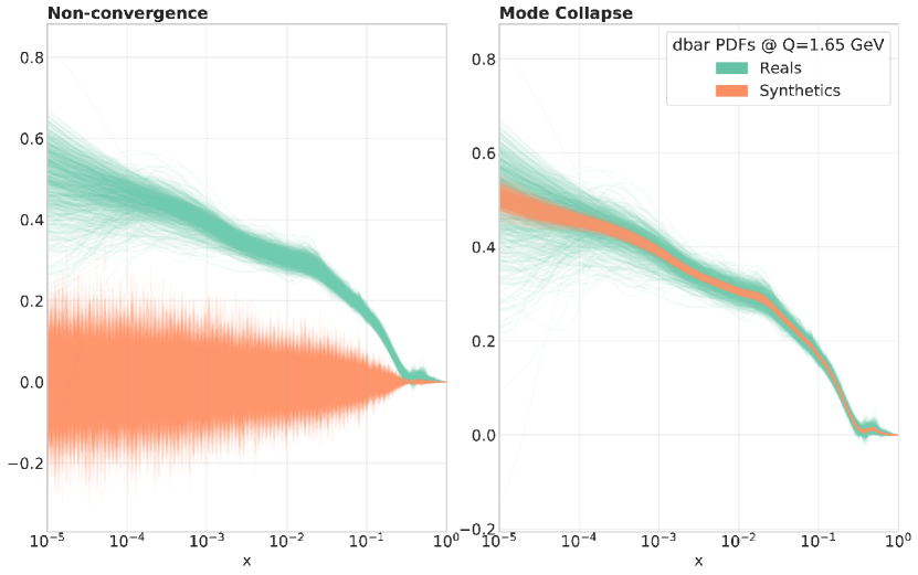
Training generative adversarial models can be very challenging due to the lack of stopping criteria that estimates when exactly GANs have finished training. Therefore, there is no guarantee that the equilibrium is reached. In addition, GANs have common failure modes due to inappropriate choices of network architecture, loss function or optimization algorithm. Several solutions have been proposed to address these issues which is a topic still subject to active research. For a review, we refer the reader to Refs. saxena2020generative ; wiatrak2020stabilizing ; 8667290 .

In this section, we describe our solutions to some of these challenges which are specific to our problem is described in the next section. The most encountered limitations of GANs in our case are: non-convergence, vanishing gradients, and mode collapse.

It is often the case that during optimization, the losses of generator and discriminator continue to oscillate without converging to a clear stopping value. Although the existence of an equilibrium has been proved in the original GAN paper goodfellow2014generative , there is no guarantee that such an equilibrium will be reached in practice. This is mainly due to the fact that the generator and discriminator are modelled in terms of neural networks, thus restricting the optimization procedures to the parameter space of the networks rather than learning directly from the probability distributions wiatrak2020stabilizing . On the other hand, this non-convergence could happen even if the models has ventured near the equilibrium point. When the generated samples are far from the target distribution, the discriminator pushes the generator towards the true data distribution while at the same time increasing its slope. When the generated samples approaches the target distribution, the discriminator’s slope is the highest, pushing away the generator from the true data distribution mescheder2018training . As a result, depending on the stopping criteria, the GAN optimization might not necessarily converge to a Nash equilibrium goodfellow2014generative in which the performance of the discriminator and generator cannot be improved further (i.e. optimal conditions). In such a scenario, the generated samples are just collections of random noise.

The vanishing gradients occur when the discriminator is over-optimized and does not provide enough information to the generator to make substantial progress saxena2020generative . During backpropagation, the gradient of the generator flows backward from the last layer to the first, getting smaller at each iteration. This raises some complications since, in practice, the objective function of a discriminator close to optimal is not $2\,\mathrm{JSD}(p_{R},p_{\theta})-2\log 2$ as stated in Eq. 5, but rather close to 0. This pushes the loss function to 0, providing little or no feedback to the generator. In such a case, the gradient does not change the values of the weights in the initial layers, altering the training of the subsequent layers.

Finally, the mode collapse occurs when the generator outputs samples of low diversity bang2018mggan , i.e, the generator maps multiple distinct input to the same output. In our case, this translates into the GAN generating PDF replicas that capture only a few of the modes of the input PDF. Mode collapse is a common pathology to all generative adversarial models as the cause is deeply rooted in the concept of GANs.

Figure 1: Illustration of non-convergence and mode collapse in the context of Monte Carlo PDF replica generation. The two plots were generated using Algorithm 1 but with different neural network architecture.

The challenges mentioned above contribute to the instabilities that arise in training GAN models. What often complicates the situation is that these obstacles are linked with each other and one might require a procedure that tackles all of them at the same time. As we will briefly describe in the next section, there exist various regularization techniques, some specific to the problem in question, that could influence the stability during the training.

3.3 The ganpdfs methodology

In this section, we describe some regularization procedures implemented in ganpdfs that alleviate the challenges mentioned in the previous section when using the standard GAN to generate Monte Carlo PDF replicas.

One of the main causes leading to unstable optimization, and therefore to non-convergence, is the low dimensional support of generated and target distributions wiatrak2020stabilizing . This could be handled by providing additional information to the input latent vector $z$ mescheder2018training . This method supplies the latent variable with relevant features of the real sample. In our case, this is done by taking a combination of the input PDF replicas, adding on top of it Gaussian noise, and using it as the latent variable. This has been shown to improve significantly the stability of the GAN during optimization.

On the other hand, it was shown in Refs. mescheder2018adversarial ; arjovsky2017principled that the objective function that the standard GAN minimizes is not continuous w.r.t. the generator’s parameters. This can lead to both vanishing gradients and mode collapse problems. Such a shortcoming was already noticed in the original GAN paper where it was shown that the Jensen-Shannon divergence under idealized conditions contributes to oscillating behaviours. As a result, a large number of studies have been devoted to finding a well defined objective function. In our implementation, we resorted to the Wasserstein or Earth’s Mover’s (EM) distance pinetz2019estimation which is implemented in Wasserstein GAN (WGAN arjovsky2017wasserstein ; gulrajani2017improved ). The EM loss function is defined in the following way:

$$\min_{\theta}\>\max_{\phi}\,V=\mathrm{E}_{x\sim p_{R}}\left(D_{\phi}(x)\right)-\mathrm{E}_{x\sim p_{\theta}}\left(D_{\phi}(x_{g})\right),$$ (6)

where again $x_{g}=G_{\theta}(z),\,z\sim p_{z}$. The EM distance metric is effective in solving vanishing gradients and mode collapse as it is continuously differentiable w.r.t. the generator and discriminator’s parameters. As a result, WGAN models result in a discriminator function whose gradients w.r.t. its input is better behaved that the standard GAN. This means that discriminator can be trained until optimality without worrying about vanishing gradients. The default GAN architecture in ganpdfs is based on WGAN and is described in Algorithm 2.

for epochs $1,\cdots,N$ do

       for discriminator steps $1,\cdots,k$ do

             - Sample minibatch of size $m$ from the real input sample: $\{x_{r}^{(1)},\cdots,x_{r}^{(m)}\}$

             - Sample minibatch of size $m$ from the custom latent space: $\{z^{(1)},\cdots,z^{(m)}\}$

             - Perform gradient ascent on discriminator:

$$\nabla_{\phi}V\left(G_{\theta},D_{\phi}\right)=\frac{1}{m}\nabla_{\phi}\sum_{i=1}^{m}\left(D_{\phi}\left(x_{r}^{(i)}\right)-D_{\phi}\left(x_{g}^{(i)}\right)\right)$$

             - $\phi=\phi+\mathrm{RMSProp}(\phi,\nabla_{\phi}V)$

             - Clip weights within $\left[-c,c\right]$

       end for

      for generator steps $1,\cdots,l$ do

             - Sample minibatch of size $m$ from the custom latent space: $\{z^{(1)},\cdots,z^{(m)}\}$

             - Perform gradient descent on generator:

$$\nabla_{\theta}V\left(G_{\theta},D_{\phi}\right)=\frac{1}{m}\nabla_{\theta}\sum_{i=1}^{m}D_{\phi}\left(x_{g}^{(i)}\right)$$

             - $\theta=\theta-\mathrm{RMSProp}(\theta,\nabla_{\theta}V)$

       end for

      

end for

Algorithm 2 Stochastic gradient descent training of the GANs implemented in ganpdfs.

Although the EM distance measure yields non-zero gradients everywhere for the discriminator, the resulting architecture can still be unstable when gradients of the loss function are large. This is addressed by clipping the weights of the discriminator to lie within a compact space defined by $\left[-c,c\right]$.

Finally, one of the factors that influence the training of GANs is the architecture of the neural networks. The choice of architecture could scale up significantly the GAN’s performance. However, coming up with values for hyper-parameters such as the size of the network or the number of nodes in a given layer is particularly challenging as the parameter space is very large. A heuristic approach designed to tackle this problem is called hyper-parameter scan or hyper-parameter optimization. Such an optimization allows for a search of the best hyper-parameters through an iterative scan of the parameter space. In our implementation, we rely on the Tree-structured Parzen Estimator (TPE) bergstra:hal-00642998 as an optimization algorithm, and we use the Fréchet Inception Distance (FID) heusel2018gans as the figure of merit to hyper-optimize on. For a target distribution with mean $\mu_{r}$ and covariance $\Sigma_{r}$ and a synthetic distribution with mean $\mu_{s}$ and covariance $\Sigma_{s}$, the FID is defined as:

$$\text{FID}=||\mu_{r}-\mu_{s}||^{2}+\text{Tr}\left(\Sigma_{r}+\Sigma_{s}-2\sqrt{\Sigma_{r}\Sigma_{s}}\right).$$ (7)

The smaller the value of the FID is, the closer the generated samples are to the target distribution. The TPE algorithm will search for sets of hyper-parameter which lead to lower values of the FID using the hyperopt pmlr-v28-bergstra13 hyper-parameter optimization tool.

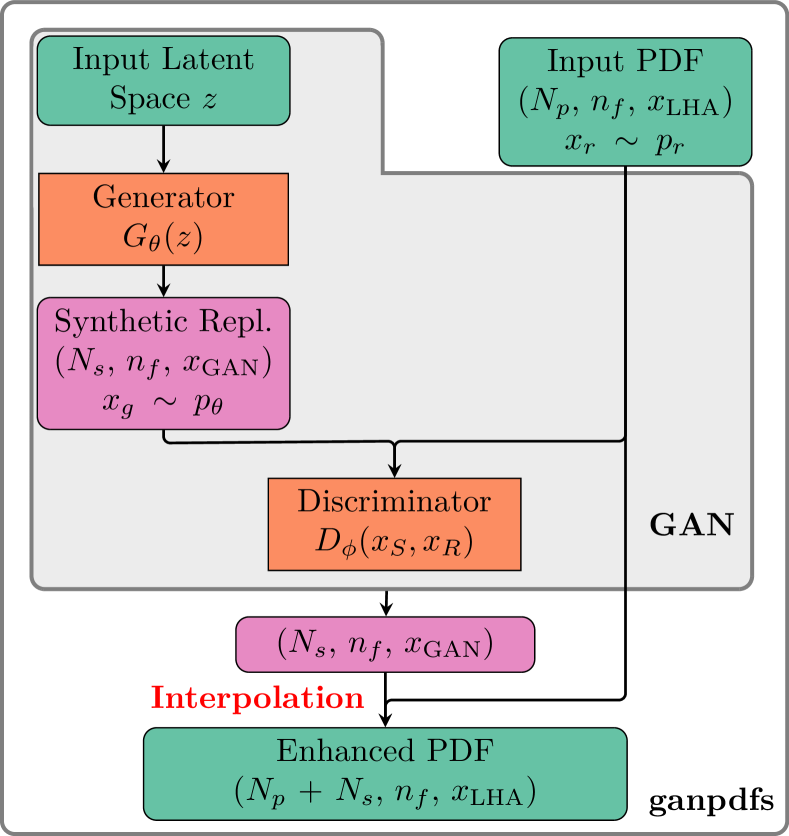
The implementation of the GAN for PDFs has been done using the machine learning framework TensorFlowtensorflow2015:whitepaper . A diagrammatic summary of the workflow is given in Fig. 2. We see that in order to train, the GAN receives as input a tensor with shape ($N_{p}$, $n_{f}$, $x_{\text{LHA}}$), where $N_{p}$ denotes the number of input replicas, $n_{f}$ the total number of flavours, and $x_{\text{LHA}}$ the size of the grid in x.

The output of ganpdfs is a LHAPDF grid Buckley:2014ana at a starting scale $Q_{0}=$1.65\text{\,}\mathrm{GeV}$$ which can then be evolved using APFEL Bertone:2013vaa to generate a full LHAPDF set of $N_{s}$ synthetic replicas. Physical constrains, such as the positivity of the PDFs or the normalization of the different flavours, are not enforced but rather inferred from the underlying distribution.

Figure 2: Flowchart describing the combined GANs and compression framework. The ganpdfs code is interfaced with the pyCompressor code from which input arguments related to the enhancement and compression are passed.

4 The GAN-enhanced compressor

Having introduced the concepts of PDF compression and generative adversarial techniques, we present in Fig. 3 a schematic diagram combining the two frameworks. The workflow goes as follows: the input PDF grid is computed for a given Monte Carlo PDF set containing $N_{p}$ replicas at fixed $Q_{0}$ and at some value of the Bjorken $x$. If GAN enhancement is not required, the reduction strategy follows the standard compression introduced in Section 2. If, on the other hand, the enhancement is required, the GAN is used to generate $N_{s}$ synthetic replicas. Notice that the format of the $x$ grid in which the GAN is trained does not have to be the same as the LHAPDF. By default, the $x_{\text{GAN}}$ is a grid of $N_{x}=500$ points logarithmically spaced in the small-$x$ region $[10^{-9},10^{-1}]$ and linearly spaced in the large-$x$ region $[10^{-1},1]$. In such a scenario, an interpolation is required in order to represent the output of the GAN in the LHAPDF format. The synthetic replicas along with the prior (enhanced set henceforth) has a total size $N_{e}=N_{p}+N_{s}$. The combined sets then passed to the pyCompressor code for compression. In the context of GAN-enhanced compression, the samples of replicas that will end up in the compressed set are drawn from the enhanced set rather than from the prior. However, since we are still trying to reproduce the probability distribution of the original PDF set, the minimization has to be performed w.r.t. the input Monte Carlo replicas. As a consequence, the expression of the error function in Eq. 1 has to be modified accordingly, i.e. computing the estimator $C$ using samples from the enhanced distribution. It is important to emphasize that the expression of the normalization factors does not change; that is, the random set of replicas have to be extracted from the prior.

Figure 3: Flowchart describing the combined GANs and compression framework. The ganpdfs code is interfaced with the pyCompressor code from which input arguments related to the enhancement and compression are passed.

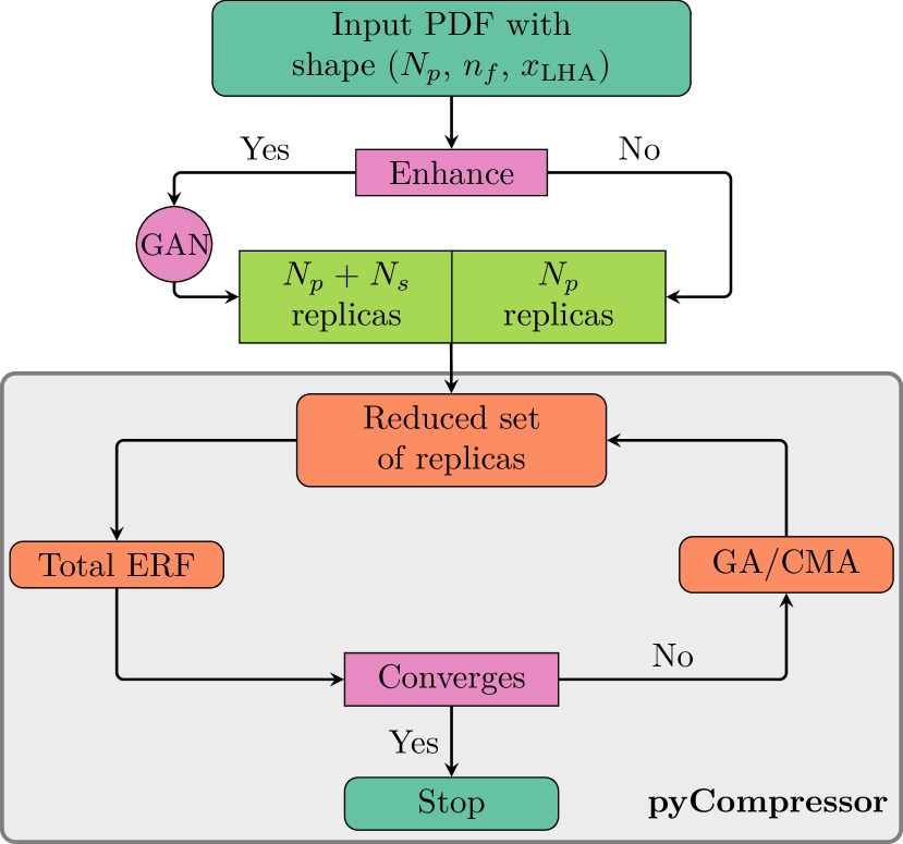
Performing a compression from an enhanced set, however, can be very challenging. Indeed, the factorial growth of the number of replicas probes the limit of the Genetic Algorithm and therefore spoils the minimization procedure. In order to address this combinatorial problem, we implemented in the compression code an adiabatic minimization procedure (see App. B for details).

Figure 4: Graphical representation of an hyper-parameter scan for a few selected parameters. On the $y$-axis is represented the different values of the FID. The violin plots represent the behaviour of the training for a given hyper-parameter. Violins with denser tails are considered better choices.

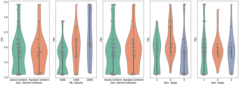
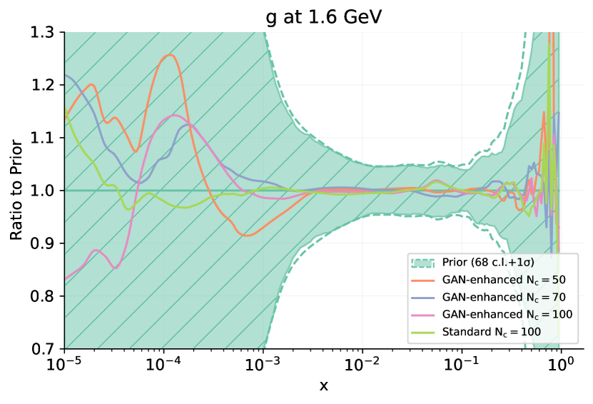
Throughout this paper, we always consider a PDF set with a prior of $N_{p}=1000$ replicas generated using the NNPDF3.1 methodology Ball:2017nwa . Plots and figures are generated using the ReportEngine-based validphys suite zahari_kassabov_2019_2571601 . We use the ganpdfs to generate $N_{s}=2000$ synthetic replicas for a total of $N_{e}=3000$ replicas. In order to reduce biases, the parameters of the GAN architecture are configured according to the results of a hyper-parameter scan. In Fig. 4, we plot an example of such a scan in which we show a few selected hyper-parameters. For each hyper-parameter, the values of the FID are plotted as a function of different parameters. The violin shapes represent a visual illustration of how a given parameter behave during the training. That is, violins with denser tails are considered better choices as they yield stable training. For instance, we can see that $1000$ epochs lead to more stable results as opposed to $1500$ or $2000$. For a complete summary, the list of hyper-parameters with the corresponding best values are shown in Table 1.

	Generator	Discriminator
Network depth	3	2
kernel initializer	glorot uniform	glorot uniform
weight clipping	-	0.01
optimizer	None	RMSprop
activation	leakyrelu	leakyrelu
steps	1	4
batch size	70$\%$
number of epochs	1000

Table 1: Parameters on which the hyper-parameter scan was performed are shown in the first column. The resulting best values are shown for both the generator and discriminator in the second and third column.

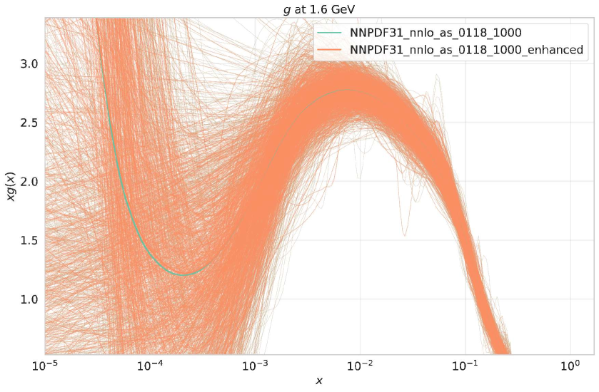
It is important to emphasize that the training of the generator has to be performed w.r.t. the discriminator’s predictions. This is the reason why no optimizer is required when training the generator. For illustration purposes, we show in Fig. 5 the output of the GANs by comparing the synthetics with the input Monte Carlo replicas.

Figure 5: Comparison of the prior Monte Carlo PDF replicas with 1000 replicas and the synthetics with 2000 replicas generated from the prior. The synthetic sample does not (explicitly) contain replicas from the prior.

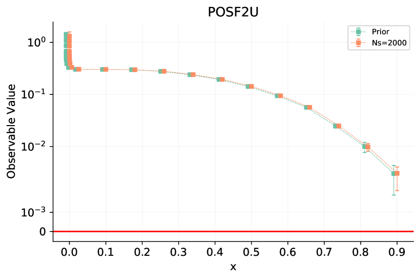
We also verify that despite the fact that physical constraints such as sum rules and positivity of the PDFs are not enforced when constructing the synthetic set, they are automatically satisfied. In Table 2 we compare the values of the sum rules between prior and synthetic replicas. We notice that the resulting values from the synthetic PDFs are very close to the ones from a real fit. Similar conclusions can be inferred when looking at the positivity plots in Fig. 6 from which we can see that not only the positivity of the PDFs are preserved in the synthetic PDFs, but also the results are quite close to the real fit.

Prior	mean	std
momentum	0.9968	$7.315\times 10^{-4}$
$u_{v}$	1.985	$3.122\times 10^{-2}$
$d_{v}$	0.9888	$3.764\times 10^{-2}$
$s_{v}$	$3.249\times 10^{-3}$	$3.547\times 10^{-2}$
Synthetic	mean	std
momentum	0.9954	$1.907\times 10^{-3}$
$u_{v}$	1.992	$3.788\times 10^{-2}$
$d_{v}$	0.9956	$3.796\times 10^{-2}$
$s_{v}$	$2.073\times 10^{-4}$	$4.833\times 10^{-2}$

Table 2: Table comparing the values of the sum rules between the prior with $N_{p}=1000$ and synthetic PDF set with $N_{s}=2000$ generated from the prior using ganpdfs.

Figure 6: Positivity constraint for the prior (green) and synthetic (orange) PDF sets. These constraints corresponds to the positivity observable $F^{u}_{2}(x)$ introduced in Eq. (14) of Ball:2014uwa .

5 Results

In this section, we quantify the performance of the GAN-enhanced compression methodology described in the previous section based on various statistical estimators. First, as a validity check, we compare the central values and luminosities of the GAN-enhanced compressed sets with the results from the original PDF set and the standard compression. Then, in order to estimate how good the GAN-compressor framework is compared to the previous methodology, we subject the compressed sets resulting from both methodologies to more visual statistical estimators such as correlations between different PDF flavours. Here, we consider the same Monte Carlo PDF sets as the ones mentioned in the previous section, namely a prior set with $N_{p}=1000$ replicas which was enhanced using ganpdfs to $N_{e}=3000$ replicas (i.e., $N_{s}=2000$ synthetic replicas). In all the cases, the compression of the PDF sets are handled by the pyCompressor code.

5.1 Validation of the GAN-compressor

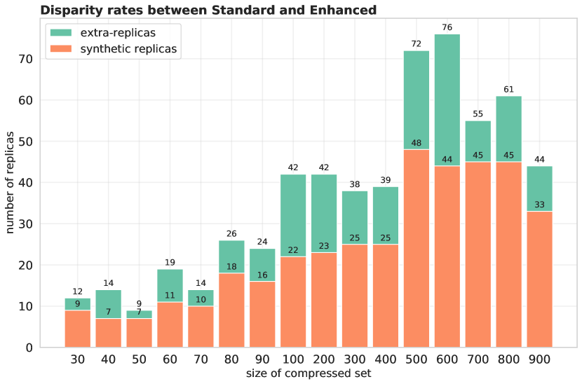
First, we would like to see, for a given compression from the enhanced set, how many replicas are selected from the synthetic set. We consider the compression of the enhanced set into subsets with smaller number of replicas. In Fig. 7, we show the disparity rate between the standard and GAN-enhanced compressed sets, i.e. the number of replicas that are present in the GAN-enhanced compressed sets (including synthetics) but not in the standard sets. We also highlight the number of synthetic replicas that end up in the final set. The results are shown for various sizes of the compressed set. For smaller sizes (smaller than $N_{c}=200$), the percentage of synthetic replicas exceeds $10\%$ and this percentage decreases as $N_{c}$ increases. This is explained by the fact that as the size of the compressed set approaches the size of the input PDF, the probability distribution of the reduced real samples get closer to the prior and fewer synthetics are required.

Figure 7: The histograms represent the number of disjoint replicas that are present in the standard compressed set but not in the GAN-enhanced for the NNPDF4.0 candidate. The results are shown as a function of the size of the compressed set. The numbers of synthetic replicas are included.

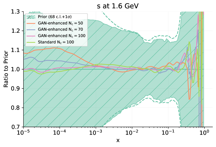
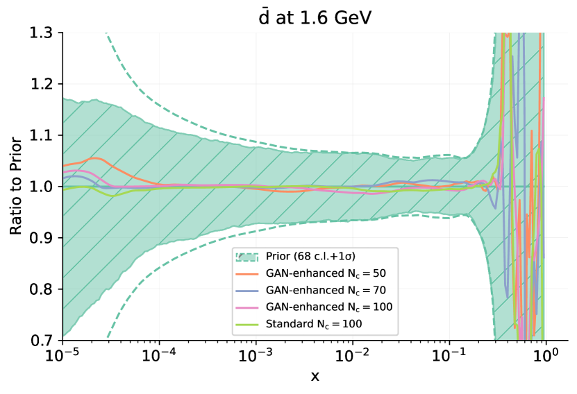
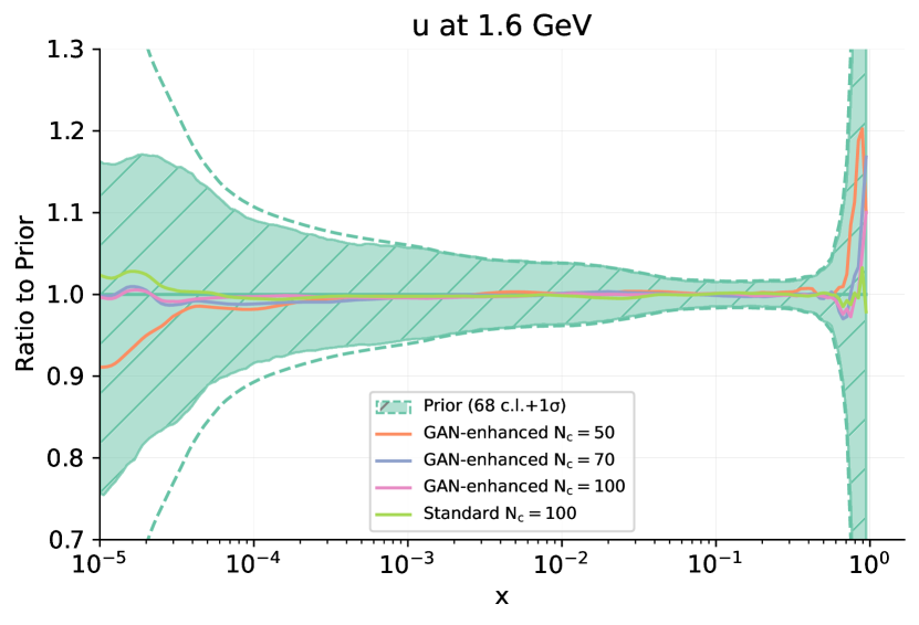
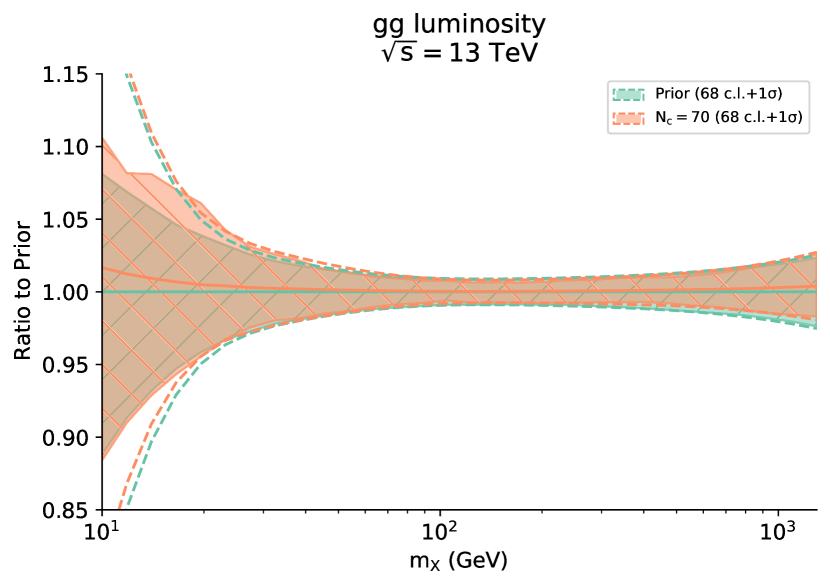
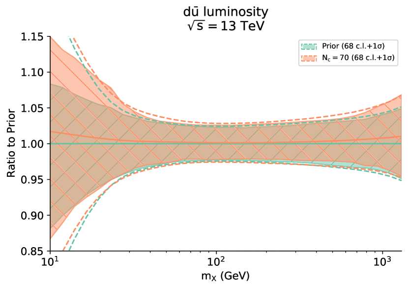
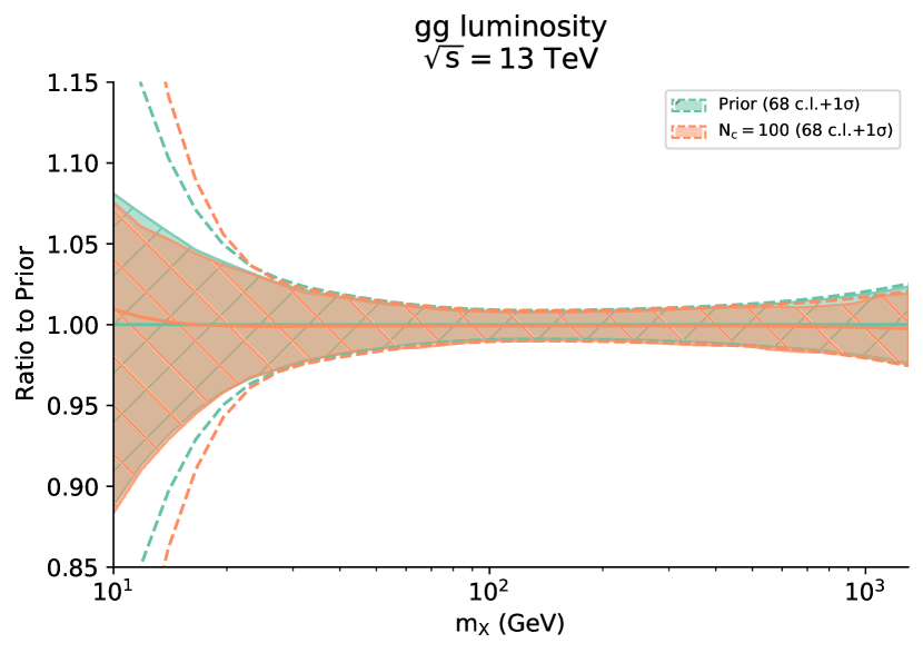
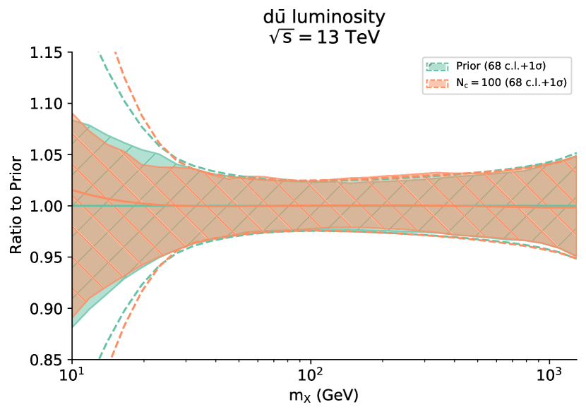
Now we turn to the validation of the GAN-enhanced compression methodology by looking at the PDF central values and luminosities. In Fig. 8, we plot the absolute central values of the reduced sets resulting from the compression of the GAN-enhanced Monte Carlo replicas at a scale $Q=$1.65\text{\,}\mathrm{GeV}$$. The results are presented for three different sizes of compressed sets $N_{c}=50,70,100$ and for various PDF flavours $(g,s,\bar{d},\bar{s})$. The results are normalized to the central value of the prior Monte Carlo PDF replicas. In order to quantify whether or not samples of $N_{c}=50,70,100$ are good representations of the probability distributions of the prior PDF replicas, we plot the $68\%$ c.l. and the 1-sigma band. We see that the PDF uncertainties are much larger than the fluctuations of the central values, indicating that a compressed set with size $N_{c}=50$ captures the main statistical properties of the prior. In Fig. 9 we plot the luminosities for the $g$-$g$, $d$-$\bar{u}$ combinations as a function of the invariant mass of the parton pair $M_{x}$ for two different compressed sizes: $N_{c}=70,100$. The error bands represent the 1-sigma confidence interval. At lower values of $M_{X}$ where PDFs are known to be non-Gaussian, the $N_{c}=70$ compressed set slightly deviate from the underlying probability distributions. However, the deviations are very small compared to the uncertainty bands. For $N_{c}=100$, we see very good agreement between the prior and the compressed set.

The above results confirm that compressed sets extracted from the GAN-enhanced compression framework fully preserve the PDF central values and luminosities. In particular, we conclude that about $50$ replicas are sufficiently enough to reproduce the main statistical properties of an input with $N_{p}=1000$ replicas. Next, we quantity how efficient the generative-based compressor strategy is compared to the standard approach.

Figure 8: Comparison of the PDF central values resulting from the GAN-enhanced compression for different values of $N_{c}$ $=50,70,100$ and different PDF flavours $(g,s,\bar{d},\bar{s})$. Results are normalized to the central value of the prior set. The $68\%$ c.l. is represented by the green hatched band while the 1-sigma is given by the dashed green curves. As a reference, results from the standard compression for $N_{c}=100$ are also shown.

Figure 9: Comparison of the PDF luminosities between the prior and the GAN-enhanced compressed sets at LHC with $\sqrt{s}=$13\text{\,}\mathrm{GeV}$$. The results are shown for different $N_{c}=70,100$ and for different PDF luminosities ($gg$ and $d\bar{u}$). The error bands represent the $68\%$ c.l.

5.2 Performance of the GAN-enhanced compressor

In order to quantify how good the GAN-compressor framework is compared to the previous methodology, we evaluate the compressed sets resulting from both methodologies on various statistical indicators. We consider the same settings as in the previous sections, namely a prior with $N_{p}=1000$ enhanced with the GAN to generate $N_{s}=2000$ synthetic replicas. The results from the GAN-enhanced compressor are then compared to the results from the standard compression in which the subset of replicas are selected directly from the prior.

Figure 10: Comparison of the best ERF values for the compression of a Monte Carlo PDF with $N_{p}=1000$ replicas. For each compressed set, we show the contribution of each of the statistical estimators that contribute to the total ERF using the standard compression (green) and the GAN-enhanced compression (orange) methodology. For illustration purposes, the mean (purple) and median (light blue) resulting from the average of $N_{r}=1000$ random selections are shown. The resulting confidence intervals from the random selections are represented by the blue $(50\%)$, green $(68\%)$, and red $(90\%)$ error bars.

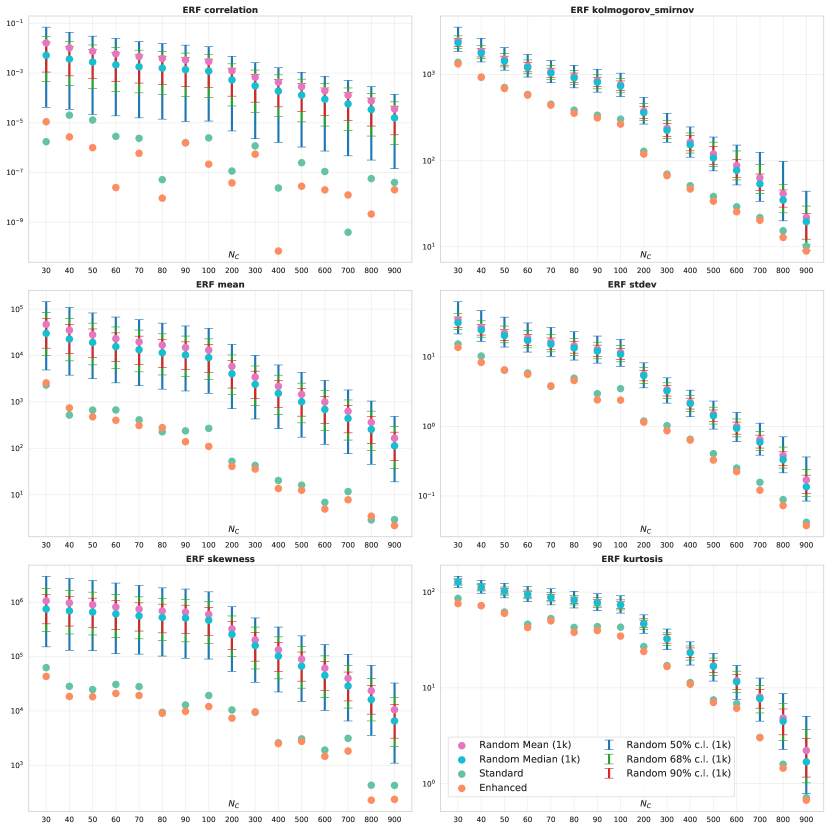
In Fig. 10, for each compressed set, we show the contribution of each statistical estimators (mean, standard deviation, Kurtosis, Skewness, Kolmogorov distance, and correlation) that contribute to the total value of the ERF using the standard (green) and GAN-based (orange) approach as a function of the size of the compressed set. For reference, we also show the mean (purple) and median (light blue) computed by taking the average ERF values from $N_{r}=1000$ random selections. The confidence intervals ($50\%,68\%,90\%$) computed from the random selections are shown as error bars of varying colours and provide an estimate of how representative of the prior distribution a given compressed set is.

First of all, we see from the plots that as the size of the compressed set increases, the ERF values for all the estimators tend to zero. On the other hand, it is clear that both compression methodologies outperform quite significantly any random selection of replicas. But in addition, by comparing the results from the standard and GAN-enhanced compression we observe that the estimators for the enhanced compression are, in all cases except for a very few, below those of the standard compression. This suggests that the GAN-enhanced approach will result in a total value of ERF that is much smaller than the one from the standard compression methodology.

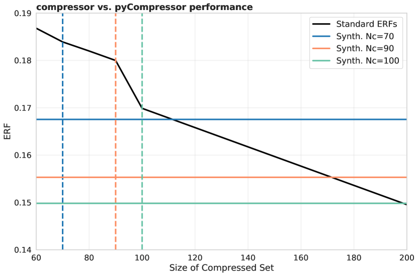
In terms of efficiency, these results imply that the GAN-enhanced methodology outperforms the standard compression approach by providing a more adequate representation of the probability distribution of the prior. This is illustrated in Fig. 11 in which we plot in solid black line the total ERF values for the standard compression as a function of the size of the compressed set. The vertical dashed lines represent the size of the compressed set $N_{c}=70,90,100$ while the horizontal solid lines represent the respective ERF values for the generative-based compression. The intersection between vertical dashed lines and horizontal solid lines below the black line indicate that the GAN-based compression outperform the standard approach. For instance, we see that $N_{c}=70$ from the enhanced compressed set is equivalent to about $N_{c}=110$ from the standard compression, and $N_{c}=90$ from the enhanced compressed set provide slightly more statistics than $N_{c}=150$ from the standard compression.

Figure 11: Comparison of the performance of the new generative-based compression algorithm (synthetic) and the the previous methodology (standard). The normalized ERF values of the standard compression are plotted as a function of the size $N_{c}$ of the compressed set (solid black line). The dashed blue, orange, and green lines represent $N_{c}=70,90,100$ respectively. The solid lines represent the corresponding ERF values of the enhanced compression.

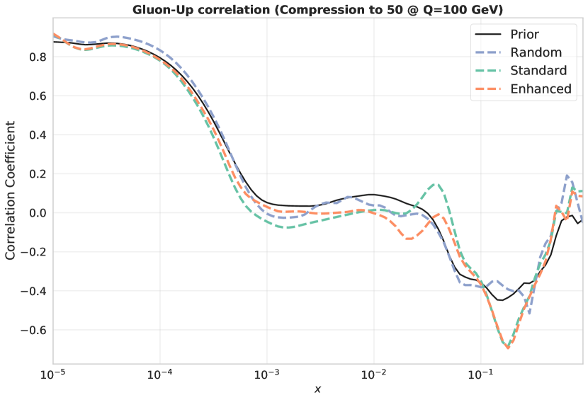
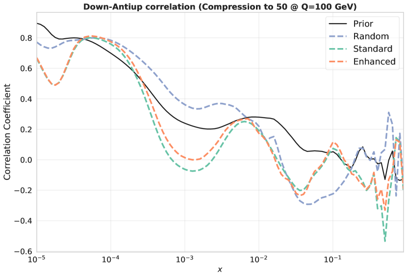
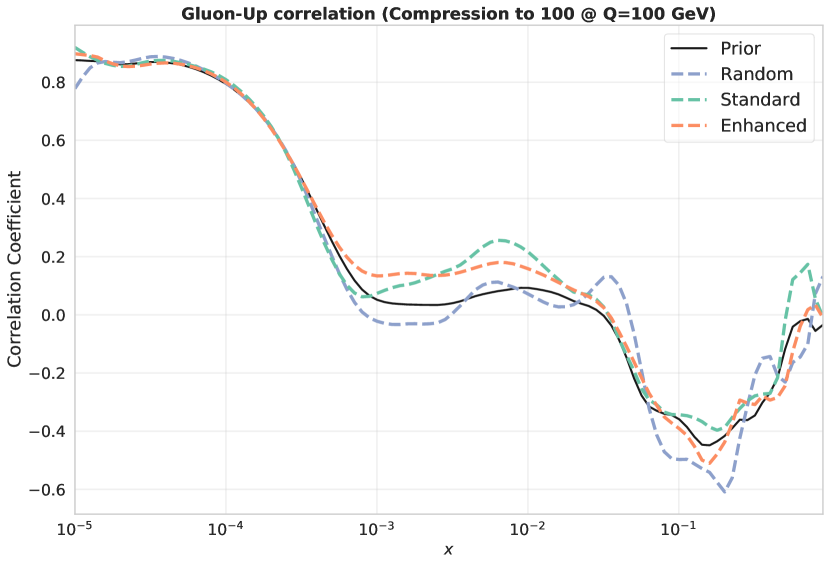
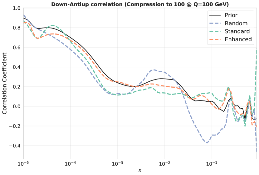
In addition to the above checks, one can also verify that correlations between PDFs are well preserved after the compression. It is important to emphasize that one of the main differences between a fit with $100$ and $1000$ Monte Carlo replicas is that correlations are reproduced more accurately in the latter Carrazza:2015hva . This is one of the main reasons why the compression methodology is important. Here, we show that for the same size of compressed set, the resulting compression from the GAN-enhanced methodology also reproduces more accurately the correlations from the prior than the standard compression. One way of checking this is to plot the correlations between two given PDFs as a function of the Bjorken variable $x$. In Fig. 12, we show the correlation between a few selected pairs of PDFs ($g$-$u$ and $d$-$\bar{u}$) for $N_{c}=50,100$ at an energy scale $Q=$100\text{\,}\mathrm{GeV}$$. The results from the GAN-enhanced compression (orange) are compared to the ones from the standard approach (green). For illustration purposes, we also show PDF correlations from sets of randomly chosen replicas (dashed black lines). We see that both compression methodologies capture very well the PDF correlations of the prior distribution. Specifically, in the case $N_{c}=100$, we see small noticeable differences between the old and new approach, with the new approach approximating best the original.

Figure 12: Correlations between $g$-$u$ and $d$-$\bar{u}$ PDFs for compressed sets with size $N_{c}=50$ (top) and $N_{c}=100$ (bottom). The energy scale $Q$ has been chosen to be $Q=$100\text{\,}\mathrm{GeV}$$. The correlation extracted from the results of the GAN-compressor (orange) is compared to the results from the standard compressor (green).

Figure 13: Difference between the correlation matrices of the prior and the compressed set resulting from the standard (first row) or enhanced (second row) compression. The correlation matrices are shown for different sizes of the compressed set: $N_{c}=50$ (first column), $N_{c}=70$ (second column), and $N_{c}=100$ (third column). The energy scale $Q$ at which which the correlations have been computed was chosen to be $Q=$100\text{\,}\mathrm{GeV}$$.

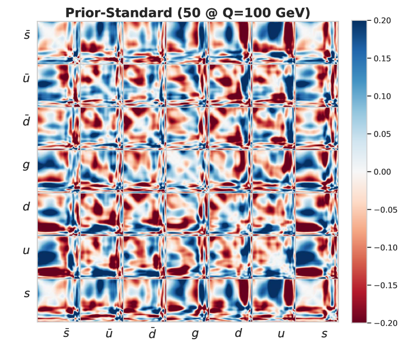
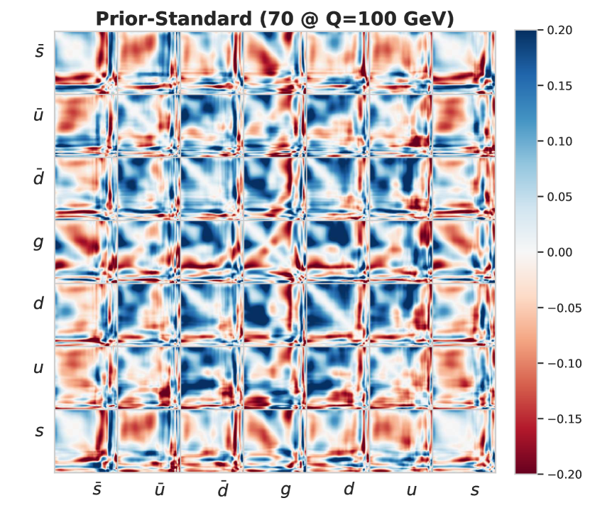
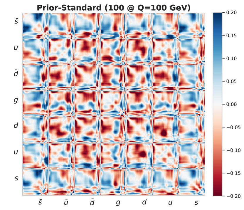
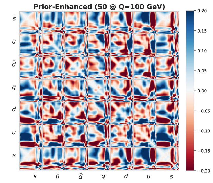
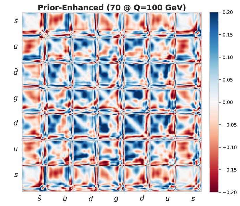
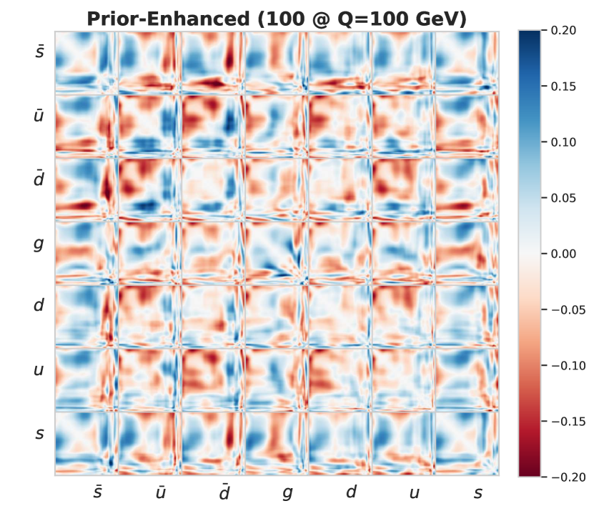
An analogous way to verify that the compressed sets resulting from the GAN-enhanced methodology reproduce more accurately the correlations of the prior PDF replicas is to compute the difference in correlation matrices. That is, compute the correlation matrix for each set (prior, standard, enhanced) and then compute the difference between the correlation matrix of the prior and the standard (or enhanced respectively). Such studies are shown in Fig. 13 where the matrices are defined in a logarithmic $x$ grid with size $N_{x}=70$ points for each of the $n_{f}=8$ light partons. The first row shows the difference between the correlation matrix of the prior and the results from the standard compression, while the second row shows the difference between the prior and the results from the generative-based compression. From the first to the third row, we present results for the compressed set with size $N_{c}=50,70,100$. As we go from left to right, we see that the correlation matrix is becoming lighter, indicating an increase in similarity between the PDF correlations. This feature is seen on both compression strategies. However, as we look from top to bottom, we can also see that the correlation matrices in the bottom row are lighter than the ones on top. Although this is barely seen in the case $N_{c}=50$, a minor difference can be seen at $N_{c}=70$ while the difference is clearly significant for $N_{c}=100$. These confirm the results in Fig. 10. Such a difference could be made more apparent by projecting the values of the difference in correlation matrices into a histograms and computing the mean and the standard deviation. Fig. 14 shows the histogram projections of the difference in correlations given in Fig. 13.

Figure 14: Histogram projection of the difference in correlation matrices given in Fig. 13. The green and orange lines represent the resulting differences for the standard and enhanced compression respectively, i.e the green lines represent the projection of the matrices in the first row of Fig. 13 while the orange lines represent the projection of those in the second row.

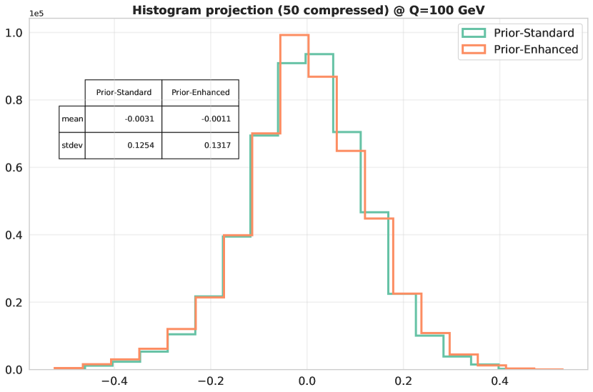
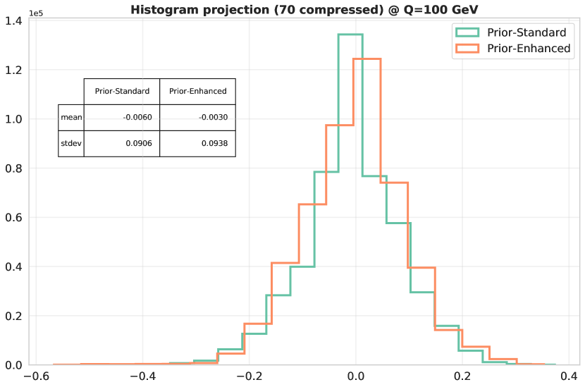
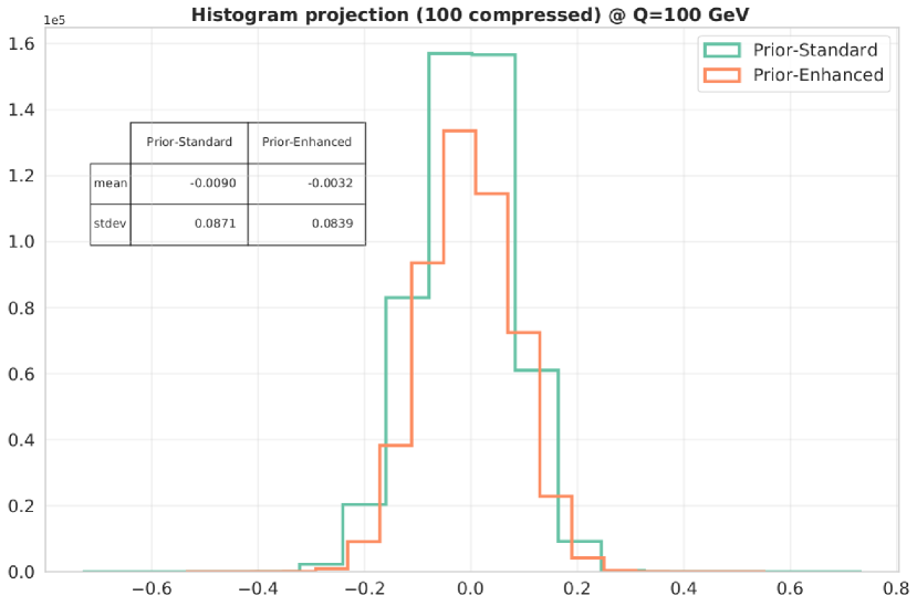
The mean and standard deviation values of the projected distributions are shown in the table on the top-left of the plots.

We see that the resulting means from the GAN-enhanced compression, for all sizes of the compressed sets, are closer to zero. This confirms the previous results that GAN-enhanced compression yields a more accurate representation of the correlations between the different partons. So far, we only focused on the role that generative-based adversarial models play in the improvement of the compression methodology. It was shown that, for all the statistical estimators we considered (including lower and higher moments, various distance metrics, and correlations), the new generative-based approach outperforms the standard compression. However, a question still remains: Can the Generative Adversarial Neural Network truly replace partly (or fully) the fitting procedure? In the next section, we try to shed some light on this question, which we hope may lie the ground to future studies.

6 Generalization capability of GANs for PDFs

Until this point, the usage of GAN has only been to reproduce, after a compression, the statistical estimators of a large set of replicas as accurately as possible. Instead, now we pose ourselves the following question: can a GAN generate synthetic replicas beyond the finite size effects of the original ensemble?

The answer to this question could potentially open two new ways of using the present framework. First, we can arbitrarily augment the density of the replicas of an existing large set in very little time. Indeed, even with the newest NNPDF methodology Carrazza_2019 , generating several thousand replicas can take weeks of computational effort. Second, once it is understood how finite-size effects affect synthetic replicas, one could, by generating as many synthetic replicas as necessary, compress a PDF set down to a minimal set which is only limited by the target accuracy even when the original set do not contain the appropriate discrete replicas (as long as the relevant statistical information is present in the prior).

As mentioned in the previous sections, the convergence of the Monte Carlo PDF to the asymptotic result depends strongly on the number of replicas (of the order of thousands). Such a large number of replicas might be feasible in future releases of NNPDF, based on the methodology presented in Ref. Carrazza_2019 . We limit ourselves here, however, to official NNPDF releases Ball:2017nwa .

We start by considering two disjoint sets of $N$ fitted replicas ($\mathrm{S}_{1}$ and $\mathrm{S}_{2}$), and a set of synthetic replicas ($\mathrm{S}_{3}$) of the same size but determined from GANs using a starting set of $N_{0}<N$ fitted replicas. Then, based on the various statistical estimators discussed previously, we measure the distance between $\mathrm{S}_{1}$ and $\mathrm{S}_{3}$ and compare the result with the distance between $\mathrm{S}_{1}$ and $\mathrm{S}_{2}$. In order to estimate the uncertainty of the distance between two subsets of replicas we need to repeat the exercise several times each time generating different subsets $\mathrm{S}_{i}$ (for $i=1,2,3$). This procedure is clearly computationally intractable. Instead, we address the problem using two resampling strategies: the (delete-1) jackknifing bradley1984use ; 10.1093/sysbio/33.4.408 ; 10.1093/sysbio/34.4.404 ; 10.1093/auk/103.2.341 and the logically similar (non-parametric) bootstrapping efron1979 ; 566814 ; 10.2307/2345699 . Both methods provide reliable estimates of the dispersion when the statistical model is not adequately known.

Figure 15: Comparison of the real and synthetic fits for various statistical estimators. The histograms are constructed by measuring the distance between $\mathrm{S}_{1}$-$\mathrm{S}_{2}$ (Reals) and $\mathrm{S}_{1}$-$\mathrm{S}_{3}$ (Synthetics). The error bars are computed by performing the delete-1 Jackknife (left) and the bootstrap resampling (right). In the bootstrap resampling, the results have been evaluated by performing $N_{B}=100$ bootstraps.

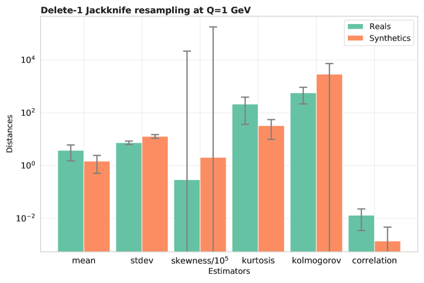
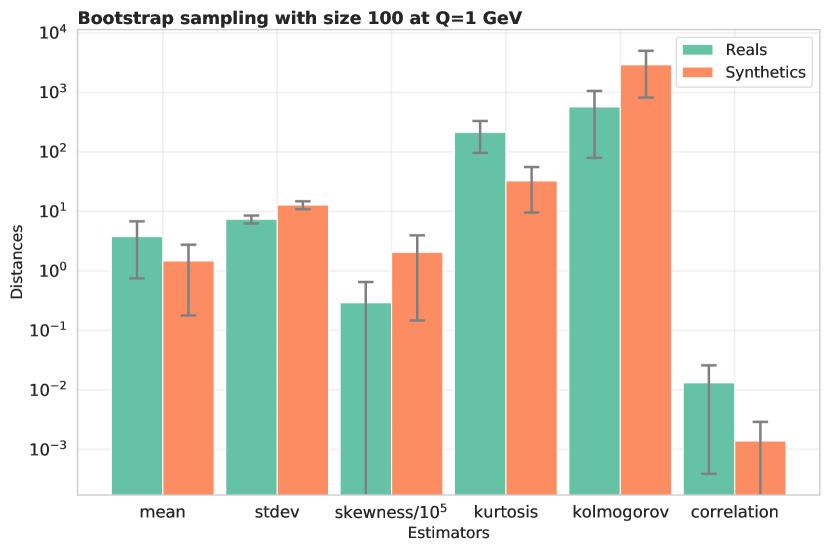
In this study the three sets $\mathrm{S}_{1}$, $\mathrm{S}_{2}$ and $\mathrm{S}_{3}$ contain each $N\!=\!500$ replicas with the difference that $\mathrm{S}_{3}$ was determined using ganpdfs from a fit with $N_{0}=100$ replicas. The results from both resampling methodologies are shown in Fig. 15. The histograms are constructed by measuring the distance between the two subsets of original replicas ($\mathrm{S}_{1}$-$\mathrm{S}_{2}$) and the distance between the synthetic replicas and one of original subsets ($\mathrm{S}_{1}$-$\mathrm{S}_{3}$). The uncertainty bars are estimated using the Jackknife resampling and the bootstrap method. From the Jackknife results, we observe that for most statistical estimators the synthetic and “true” fits produce results which are compatible within uncertainties. This is further confirmed by the results obtained through bootstrap resampling where only the error bands for the standard deviation of the two sets do not overlap.

Given that inspecting Fig. 15 it is difficult to distinguish the two sets $\mathrm{S}_{2}$ and $\mathrm{S}_{3}$ we hypothesize that this would also be the case for larger sets. If true, the present framework could be used in any of the ways proposed at the beginning of the section. We leave this for future work.

7 Conclusions

In this paper, we applied the generative adversarial strategies to the study of Parton Distribution Functions. Specifically, we showed how such techniques could be used to improve the efficiency of the compression methodology which is used to reduce the number of replicas while preserving the same statistics. The implementation of the GAN methodology required us to re-design the previously used compressor code into a more efficient one.

It was shown that with the same size of compressed set, the GAN-enhanced compression methodology achieves a more accurate representation of the underlying probability distribution than the standard compression. This is due to the generation of synthetic replicas which increases the density of the replicas for the compressor to choose from, reducing finite size effects.

Finally, in Section 6 we entertain the idea of utilising these techniques in order to generate larger PDF sets with reduced finite size effects. We have compared real and synthetic Monte Carlo replicas using two different resampling techniques and found that a GAN-enhanced set of replicas is statistically compatible with actual replicas. However, further work is needed before synthetic PDFs can be used for precision studies. This basically entails reproducing the same studies done here but with much larger samples in order to reduce statistical fluctuations.

Appendix A Benchmark of pycompressor against compressor

Among the benefits of the new code is the gain in performance. For the purpose of quantifying this gain, we compress a Monte Carlo PDF set with $N_{p}=1000$ replicas into sets with smaller sizes using the same GA in the new and old codes. The tests were run on a consumer-grade CPU (AMD Ryzen 5 2600 with 12 threads boosted at 3.4 GHz) with 16 GB of memory. The results of the benchmark are shown in Fig. 16. The plots show the required time for both compressor and pyCompressor to complete the same task. We see that the pyCompressor code is faster than the previous implementation and that, as the size of the compressed set grows, the difference in speed between the two implementations also increases. This is mainly due to the fact that the new code automatically takes advantage of the multicore capabilities of most modern computers.

Figure 16: Speed benchmark comparing the compresssor and pyCompressor codes using the GA as a minimization for $1500$ iterations. For the purpose of this benchmarks, the parameters that enter into the GA are chosen to be exactly the same across both implementations.

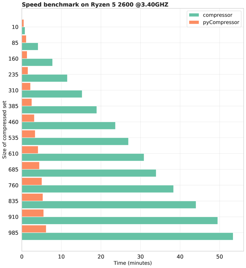
On the flip side, parallelization comes at the expense of a slightly higher memory usage (as shown in Table 3), while not dramatic it can be a burden for very high number of replicas.

	Nb. Threads	RAM usage (GB)
compressor	1	1
pyCompressor	12	2.5

Table 3: Comparison of average computing resources between ours and the previous implementation when compressing to $N_{c}=500$ replicas from a prior with $1000$ Monte Carlo PDF replicas.

Appendix B Adiabatic Minimization

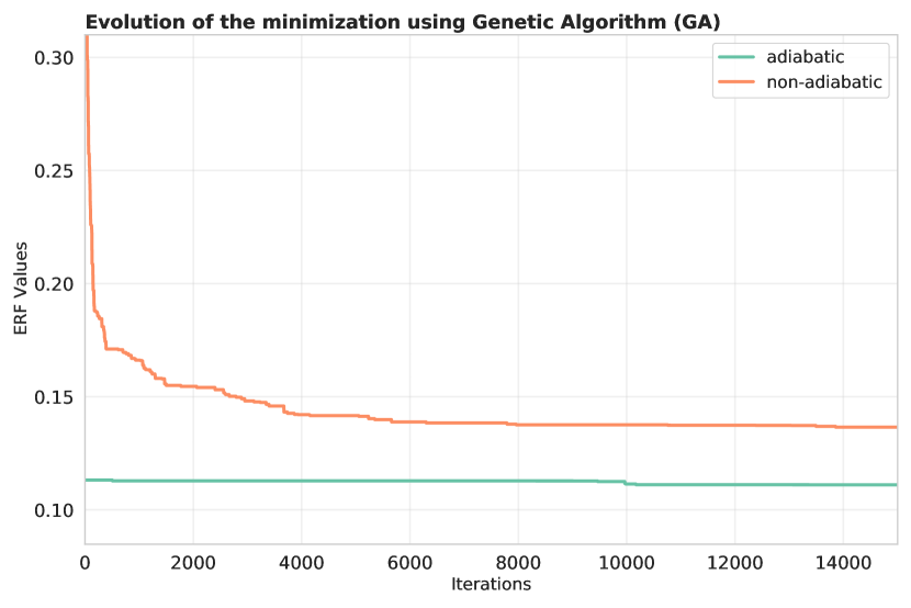
Performing a compression from an enhanced set can be challenging due to the limitation of the minimization algorithm. However, if results from the standard compression are already provided, the compressor code provides a more efficient compression procedure from the enhanced set with the means of an adiabatic minimization. The adiabatic minimization for the enhanced compression consists on taking as a starting point the space of replicas where the best from the standard compression was generated. Such a minimization not only yields faster convergence (as shown in Fig. 17), but also prevent the minimization algorithm to be trapped in some local minimum in case the enhanced set contains statistical fluctuations.

Figure 17: Comparison between adiabatic and standard minimization using the Genetic Algorithm (GA). The adiabatic minimization reaches stability faster while the standard minimization approach has not converged yet even at 15000 iterations.

References

- (1) M. Cepeda et al., CERN Yellow Rep. Monogr. 7, 221 (2019), 1902.00134
- (2) R.D. Ball et al. (NNPDF), Eur. Phys. J. C 77, 663 (2017), 1706.00428
- (3) S. Bailey, T. Cridge, L.A. Harland-Lang, A.D. Martin, R.S. Thorne (2020), 2012.04684
- (4) T.J. Hou et al. (2019), 1908.11238
- (5) S. Alekhin, J. Blumlein, S. Moch, Phys. Rev. D 89, 054028 (2014), 1310.3059
- (6) S. Carrazza, J.I. Latorre, J. Rojo, G. Watt, A compression algorithm for the combination of pdf sets (2015), 1504.06469
- (7) J.R. Andersen et al., Les Houches 2015: Physics at TeV Colliders Standard Model Working Group Report, in 9th Les Houches Workshop on Physics at TeV Colliders (2016), 1605.04692
- (8) J. Butterworth et al., J. Phys. G 43, 023001 (2016), 1510.03865
- (9) I. Goodfellow, J. Pouget-Abadie, M. Mirza, B. Xu, D. Warde-Farley, S. Ozair, A. Courville, Y. Bengio, Generative Adversarial Nets, in Advances in Neural Information Processing Systems, edited by Z. Ghahramani, M. Welling, C. Cortes, N. Lawrence, K.Q. Weinberger (Curran Associates, Inc., 2014), Vol. 27
- (10) J.Y. Zhu, T. Park, P. Isola, A.A. Efros, Unpaired image-to-image translation using cycle-consistent adversarial networks (2020), 1703.10593
- (11) L. de Oliveira, M. Paganini, B. Nachman, Comput. Softw. Big Sci. 1, 4 (2017), 1701.05927
- (12) M. Paganini, L. de Oliveira, B. Nachman, Phys. Rev. D 97, 014021 (2018), 1712.10321
- (13) A. Butter, T. Plehn, R. Winterhalder (2019), 1912.08824
- (14) M. Bellagente, A. Butter, G. Kasieczka, T. Plehn, R. Winterhalder, SciPost Phys. 8, 070 (2020), 1912.00477
- (15) A. Butter, T. Plehn, R. Winterhalder, SciPost Phys. 7, 075 (2019), 1907.03764
- (16) S. Carrazza, F.A. Dreyer, Eur. Phys. J. C 79, 979 (2019), 1909.01359
- (17) M. Backes, A. Butter, T. Plehn, R. Winterhalder (2020), 2012.07873
- (18) A. Butter, T. Plehn (2020), 2008.08558
- (19) A. Butter, S. Diefenbacher, G. Kasieczka, B. Nachman, T. Plehn (2020), 2008.06545
- (20) K.T. Matchev, P. Shyamsundar (2020), 2002.06307
- (21) S.C. T. Rabemananjara, J. Cruz-Martinez, pycompressor: A python package for monte carlo pdf compression (2020), https://doi.org/10.5281/zenodo.4616385
- (22) S.C. T. Rabemananjara, J. Cruz-Martinez, ganpdfs: A python package for pdf generation using gans (2020), https://doi.org/10.5281/zenodo.4616369
- (23) I.J. Goodfellow, J. Pouget-Abadie, M. Mirza, B. Xu, D. Warde-Farley, S. Ozair, A. Courville, Y. Bengio, Generative adversarial networks (2014), 1406.2661
- (24) M. Arjovsky, S. Chintala, L. Bottou, Wasserstein gan (2017), 1701.07875
- (25) A. Brock, J. Donahue, K. Simonyan, Large scale gan training for high fidelity natural image synthesis (2019), 1809.11096
- (26) A. Radford, L. Metz, S. Chintala, Unsupervised representation learning with deep convolutional generative adversarial networks (2016), 1511.06434
- (27) D. Saxena, J. Cao, Generative adversarial networks (gans): Challenges, solutions, and future directions (2020), 2005.00065
- (28) M. Wiatrak, S.V. Albrecht, A. Nystrom, Stabilizing generative adversarial networks: A survey (2020), 1910.00927
- (29) Z. Pan, W. Yu, X. Yi, A. Khan, F. Yuan, Y. Zheng, IEEE Access 7, 36322 (2019)
- (30) L. Mescheder, A. Geiger, S. Nowozin, Which training methods for gans do actually converge? (2018), 1801.04406
- (31) D. Bang, H. Shim, Mggan: Solving mode collapse using manifold guided training (2018), 1804.04391
- (32) L. Mescheder, S. Nowozin, A. Geiger, Adversarial variational bayes: Unifying variational autoencoders and generative adversarial networks (2018), 1701.04722
- (33) M. Arjovsky, L. Bottou, Towards principled methods for training generative adversarial networks (2017), 1701.04862
- (34) T. Pinetz, D. Soukup, T. Pock, On the estimation of the wasserstein distance in generative models (2019), 1910.00888
- (35) I. Gulrajani, F. Ahmed, M. Arjovsky, V. Dumoulin, A. Courville, Improved training of wasserstein gans (2017), 1704.00028
- (36) J. Bergstra, R. Bardenet, Y. Bengio, B. Kégl, Algorithms for Hyper-Parameter Optimization, in 25th Annual Conference on Neural Information Processing Systems (NIPS 2011), edited by J. Shawe-Taylor, R. Zemel, P. Bartlett, F. Pereira, K. Weinberger (Neural Information Processing Systems Foundation, Granada, Spain, 2011), Vol. 24 of Advances in Neural Information Processing Systems, https://hal.inria.fr/hal-00642998
- (37) M. Heusel, H. Ramsauer, T. Unterthiner, B. Nessler, S. Hochreiter, Gans trained by a two time-scale update rule converge to a local nash equilibrium (2018), 1706.08500
- (38) J. Bergstra, D. Yamins, D. Cox, Making a Science of Model Search: Hyperparameter Optimization in Hundreds of Dimensions for Vision Architectures, in Proceedings of the 30th International Conference on Machine Learning, edited by S. Dasgupta, D. McAllester (PMLR, Atlanta, Georgia, USA, 2013), Vol. 28 of Proceedings of Machine Learning Research, pp. 115–123, http://proceedings.mlr.press/v28/bergstra13.html
- (39) M. Abadi, A. Agarwal, P. Barham, E. Brevdo, Z. Chen, C. Citro, G.S. Corrado, A. Davis, J. Dean, M. Devin et al., TensorFlow: Large-scale machine learning on heterogeneous systems (2015), software available from tensorflow.org, http://tensorflow.org/
- (40) A. Buckley, J. Ferrando, S. Lloyd, K. Nordström, B. Page, M. Rüfenacht, M. Schönherr, G. Watt, Eur. Phys. J. C 75, 132 (2015), 1412.7420
- (41) V. Bertone, S. Carrazza, J. Rojo, Comput. Phys. Commun. 185, 1647 (2014), 1310.1394
- (42) Z. Kassabov, Reportengine: A framework for declarative data analysis (2019), https://doi.org/10.5281/zenodo.2571601
- (43) R.D. Ball et al. (NNPDF), JHEP 04, 040 (2015), 1410.8849
- (44) S. Carrazza, J. Cruz-Martinez, The European Physical Journal C 79 (2019)
- (45) D. BRADLEY, R. LANDRY, C. COLLINS, The Use of Jackknife Confidence Intervals with the Richards Curve for Describing Avian Growth Patterns (1984)
- (46) A.R. Gibson, A.J. Baker, A. Moeed, Morphometric Variation in Introduced Populations of the Common Myna (Acridotheres tristis): An Application of the Jackknife to Principal Component Analysis (1984), https://doi.org/10.1093/sysbio/33.4.408
- (47) S.M. Lanyon, Molecular Perspective on Higher-Level Relationships in the Tyrannoidea (Aves) (1985), https://doi.org/10.1093/sysbio/34.4.404
- (48) W.E. Lanyon, S.M. Lanyon, Generic Status of Euler’s Flycatcher: A Morphological and Biochemical Study (1986), https://doi.org/10.1093/auk/103.2.341
- (49) B. Efron, Bootstrap methods: Another look at the jackknife (1979), https://doi.org/10.1214/aos/1176344552
- (50) Y. Hamamoto, S. Uchimura, S. Tomita, IEEE Transactions on Pattern Analysis and Machine Intelligence 19, 73 (1997)
- (51) T.J. Diciccio, J.P. Romano, A review of bootstrap confidence intervals (1988)