Neural RGB-D Surface Reconstruction

Abstract

Obtaining high-quality 3D reconstructions of room-scale scenes is of paramount importance for upcoming applications in AR or VR. These range from mixed reality applications for teleconferencing, virtual measuring, virtual room planing, to robotic applications. While current volume-based view synthesis methods that use neural radiance fields (NeRFs) show promising results in reproducing the appearance of an object or scene, they do not reconstruct an actual surface. The volumetric representation of the surface based on densities leads to artifacts when a surface is extracted using Marching Cubes, since during optimization, densities are accumulated along the ray and are not used at a single sample point in isolation. Instead of this volumetric representation of the surface, we propose to represent the surface using an implicit function (truncated signed distance function). We show how to incorporate this representation in the NeRF framework, and extend it to use depth measurements from a commodity RGB-D sensor, such as a Kinect. In addition, we propose a pose and camera refinement technique which improves the overall reconstruction quality. In contrast to concurrent work on integrating depth priors in NeRF which concentrates on novel view synthesis, our approach is able to reconstruct high-quality, metrical 3D reconstructions.

1 Introduction

Research on neural networks for scene representations and image synthesis has made impressive progress in recent years [73]. Methods that learn volumetric representations [48, 42] from color images captured by a smartphone camera can be employed to synthesize near photo-realistic images from novel viewpoints. While the focus of these methods lies on the reproduction of color images, they are not able to reconstruct metric and clean (noise-free) meshes. To overcome these limitations, we show that there is a significant advantage in taking additional range measurements from consumer-level depth cameras into account. Inexpensive depth cameras are broadly accessible and are also built into modern smartphones. While classical reconstruction methods [9, 33, 53] that purely rely on depth measurements struggle with the limitations of physical sensors (noise, limited range, transparent objects, etc.), a neural radiance field-based reconstruction formulation allows to also leverage the dense color information. Methods like BundleFusion [14] take advantage of color observations to compute sparse SIFT [44] features for re-localization and refinement of camera poses (loop closure). For the actual geometry reconstruction (volumetric fusion), only the depth maps are taken into account. Missing depth measurements in these maps, lead to holes and incomplete geometry in the reconstruction. This limitation is also shared by learned surface reconstruction methods that only rely on the range data [47, 67]. In contrast, our method is able to reconstruct geometry in regions where only color information is available. Specifically, we adapt the neural radiance field (NeRF) formulation of Mildenhall et al. [48] to learn a truncated signed distance field (TSDF), while still being able to leverage differentiable volumetric integration for color reproduction. To compensate for noisy initial camera poses which we compute based on the depth measurements, we jointly optimize our scene representation network with the camera poses. The implicit function represented by the scene representation network allows us to predict signed distance values at arbitrary points in space which is used to extract a mesh using Marching Cubes.

Concurrent work that incorporates depth measurements in NeRF focuses on novel view synthesis [16, 49, 81], and uses the depth prior to restrict the volumetric rendering to near-surface regions [81, 49] or adds an additional constraint on the depth prediction of NeRF [16]. NeuS [76] is also a concurrent work on novel view synthesis which uses a signed distance function to represent the geometry, but takes only RGB images as input, and thus fails to reconstruct the geometry of featureless surfaces, like white walls. In contrast, our method aims for high-quality 3D reconstructions of room-scale scenes using an implicit surface representation and direct SDF-based losses on the input depth maps. Comparisons to state-of-the-art scene reconstruction methods show that our approach improves the quality of geometry reconstructions both qualitatively and quantitatively.

In summary, we propose an RGB-D based scene reconstruction method that leverages both dense color and depth observations. It is based on an effective incorporation of depth measurements into the optimization of a neural radiance field using a signed distance-based surface representation to store the scene geometry. It is able to reconstruct geometry detail that is observed by the color images, but not visible in the depth maps. In addition, our pose and camera refinement technique is able to compensate for misalignments in the input data, resulting in state-of-the-art reconstruction quality which we demonstrate on synthetic as well as on real data from ScanNet [12].

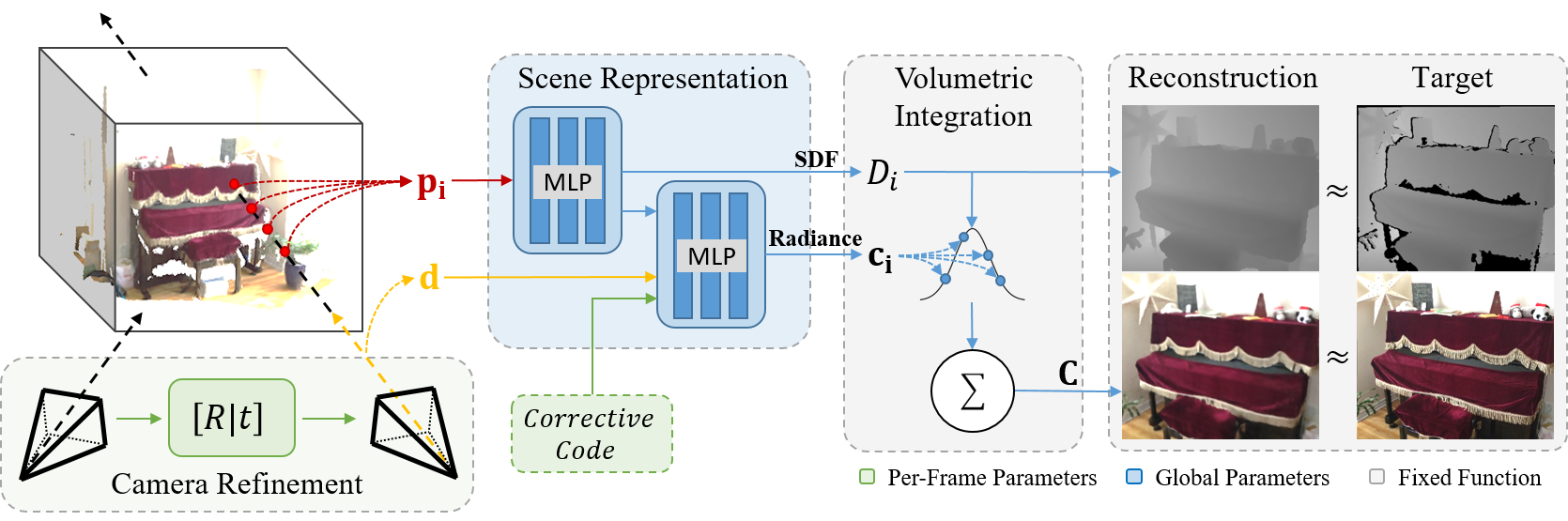
Figure 2: Differentiable volumetric rendering is used to reconstruct a scene that has been captured using an RGB-D camera. The scene is represented using multi-layer perceptrons (MLPs), encoding a signed distance value $D_{i}$ and a viewpoint-dependent radiance value $\textbf{c}_{i}$ per point $\textbf{p}_{i}$. We perform volumetric rendering by integrating the radiance along a ray, weighing the samples as a function of their signed distance $D_{i}$ and their visibility. We also learn a per-frame latent corrective code to account for exposure or white balance changes throughout the capture, which is passed to the radiance MLP alongside the ray direction d. We optimize the scene representation’s MLPs, together with the per-frame corrective codes, the input camera poses, and an image-plane deformation field (not shown) by computing losses for the signed distance $D_{i}$ of the samples, and the final integrated color C with respect to the input depth and color views.

2 Related Work

Our approach reconstructs geometry from a sequence of RGB-D frames, leveraging both dense color and depth information. It is related to classical fusion-based 3D reconstruction methods [93, 9, 50, 53, 14], learned 3D reconstruction [47, 58, 7, 15, 79], as well as to recent coordinate-based scene representation models [69, 48, 74].

Classical 3D Reconstruction.

There exists a wide range of methods for RGB and RGB-D based 3D reconstruction that are not based on deep learning. Reconstructing objects and scenes can be done using passive stereo systems that rely on stereo matching from two or multiple color views [62, 29], Structure-from-Motion [63], or SLAM-based [21, 20, 23] methods. These approaches may use disjoint representations, like oriented patches [25], volumes [38], or meshes [32] to reconstruct the scene or object. Zollhöfer et al. [93] review the 3D reconstruction methods that rely on range data from RGB-D cameras like the Kinect. Most of these methods are based on [9], where multiple depth measurements are fused using a signed distance function (SDF) which is stored in a uniform 3D grid. E.g., KinectFusion [50] combines such representation with real-time tracking to reconstruct objects and small scenes in real-time. To handle large scenes Nießner et al. [53] propose a memory-efficient storage of the SDF grid using spatial hashing. To handle the loop closure problem when scanning large-scale scenes, bundle adjustment can be used to refine the camera poses [14]. In addition, several regularization techniques have been proposed to handle outliers during reconstruction [89, 61, 19].

Deep Learning for 3D Reconstruction.

To reduce artifacts from classical reconstruction methods, a series of methods was proposed that use learned spatial priors to predict depth maps from color images [39, 28, 24], to learn multi-view stereo using 3D CNNs on voxel grids [34, 82, 68], or multi-plane images [22], to reduce the influence of noisy depth values [79], to complete incomplete scans [13, 15], to learn image features for SLAM [2, 91, 10] or feature fusion [80, 71, 4], to predict normals [90], or to predict objects or parts of a room from single images [27, 51, 11, 75, 18]. Most recently coordinate-based models have become popular [74]. These models use a scene representation that is based on a deep neural network with fully connected layers, i.e., a multi-layer perceptron (MLP) [73, 74]. As input the MLP takes a 3D location in the model space and outputs for example, occupancy [47, 58, 7, 59, 60, 52, 55], density [48], radiance [48], color [54], or the signed distance to the surface [56, 84, 83]. Scene Representation Networks [69] combine such a representation with a learned renderer which is inspired by classical sphere tracing, to reconstruct objects from single RGB images. Instead, Mildenhall et al. [48] propose a method that represents a scene as a neural radiance field (NeRF) using a coordinate-based model, and a classical, fixed volumetric rendering formulation [46]. Based on this representation, they show impressive novel view synthesis results, while only requiring color input images with corresponding camera poses and intrinsics. Besides the volumetric image formation, a key component of the NeRF technique is a positional encoding layer, that uses sinusoidal functions to improve the learning properties of the MLP. In follow-up work, alternatives to the positional encoding were proposed, such as Fourier features [72] or sinusoidal activation layers [67]. NeRF has been extended to handle in-the-wild data with different lighting and occluders [45], dynamic scenes [40, 57], avatars [26], and adapted for generative modeling [5, 66] and image-based rendering [87, 77]. Others have focused on resectioning a camera given a learned NeRF [85], and optimizing for the camera poses while learning a NeRF [78, 41].

In our work, we take advantage of the volumetric rendering of NeRF and propose the usage of a hybrid scene representation that consists of an implicit surface representation (SDF) and a volumetric radiance field. We incorporate depth measurements in this formulation to achieve robust and metric 3D reconstructions. In addition, we propose a camera refinement scheme to further improve the quality of the reconstruction. In contrast to NeRF which uses a density based volumetric representation of the scene, our implicit surface representation leads to high quality geometry estimates of entire scenes.

Concurrent Work.

In concurrent work, Wang et al. [76] present NeuS which uses an implicit surface representation to improve novel view synthesis of NeRF. Wei et al. [81] propose a multi-view stereo approach to estimate dense depth maps which they use to constrain the sampling region when optimizing a NeRF. Similarly, Neff et al. [49] restrict the volumetric rendering to near surface regions. Additional constraints on the depth predictions of NeRF were proposed by Deng et al. [16]. In contrast to these, our method focuses on accurate 3D reconstructions of room-scale scenes, with explicit incorporation of depth measurements using an implicit surface representation.

3 Method

We propose an optimization-based approach for geometry reconstruction from an RGB-D sequence of a consumer-level camera (e.g., a Microsoft Kinect). We leverage both the $N$ color frames $\mathcal{I}_{i}$ as well as the corresponding aligned depth frames $\mathcal{D}_{i}$ to optimize a coordinate-based scene representation network. Specifically, our hybrid scene representation consists of an implicit surface representation based on a truncated signed distance function (TSDF) and a volumetric representation for the radiance. As illustrated in Fig. 2, we use differentiable volumetric integration of the radiance values [46] to compute color images from this representation. Besides the scene representation network, we optimize for the camera poses and intrinsics. We initialize the camera poses $\mathcal{T}_{i}$ using BundleFusion [14]. At evaluation time, we use Marching Cubes [43] to extract a triangle mesh from the optimized implicit scene representation.

3.1 Hybrid Scene Representation

Our method is built upon a hybrid scene representation which combines an implicit surface representation with a volumetric appearance representation. Specifically, we implement this representation using a multi-layer perceptron (MLP) which can be evaluated at arbitrary positions $\textbf{p}_{i}$ in space to compute a truncated signed distance value $D_{i}$ and view-dependent radiance value $\textbf{c}_{i}$. As a conditioning to the MLP, we use a sinusoidal positional encoding $\gamma(\cdot)$ [48] to encode the 3D query point $\textbf{p}_{i}$ and the viewing direction d.

Inspired by the recent success of volumetric integration in neural rendering [48], we render color as a weighted sum of radiance values along a ray. Instead of computing the weights as probabilities of light reflecting at a given sample point based on the density of the medium [48], we compute weights directly from signed distance values as the product of two sigmoid functions:

$$w_{i}=\sigma\left(\frac{D_{i}}{tr}\right)\cdot\sigma\left(-\frac{D_{i}}{tr}\right),$$ (1)

where $tr$ is the truncation distance. This bell-shaped function has its peak at the surface, i.e., at the zero-crossing of the signed distance values. A similar formulation is used in concurrent work [76], since this function produces unbiased estimates of the signed distance field. The truncation distance $tr$ directly controls how quickly the weights fall to zero as the distance from the surface increases. To account for the possibility of multiple intersections, weights of samples beyond the first truncation region are set to zero. The color along a specific ray is approximated as a weighted sum of the $K$ sampled colors:

$$\textbf{C}=\frac{1}{\sum_{i=0}^{K-1}w_{i}}\sum_{i=0}^{K-1}w_{i}\cdot\textbf{c}_{i}.$$ (2)

This scheme gives the highest integration weight to the point on the surface, while points farther away from the surface have lower weights. Although such an approach is not derived from a physically-based rendering model, as is the case with volumetric integration over density values, it represents an elegant way to render color in a signed distance field in a differentiable manner, and we show that it helps deduce depth values through a photometric loss (see Sec. 4). In particular, this approach allows us to predict hard boundaries between occupied and free space which results in high-quality 3D reconstructions of the surface. In contrast, density-based models [48] can introduce semi-transparent matter in front of the actual surface to represent view-dependent effects when integrated along a ray. This leads to noisy reconstructions and artifacts in free space, as can be seen in Sec. 4.

Network Architecture

Our hybrid scene representation network is composed of two MLPs which represent the shape and radiance, as depicted in Fig. 2. The shape MLP takes the encoding of a queried 3D point $\gamma(\textbf{p})$ as input and outputs the truncated signed distance $D_{i}$ to the nearest surface. The task of the second MLP is to produce the surface radiance for a given encoded view direction $\gamma(\textbf{d})$ and an intermediate feature output of the shape MLP. The view vector conditioning allows our method to deal with view-dependent effects like specular highlights, which would otherwise have to be modeled by deforming the geometry. Since color data is often subject to varying exposure or white-balance, we learn a per-frame latent corrective code vector as additional input to the radiance MLP [45].

Pose and Camera Refinement

The camera poses $\mathcal{T}_{i}$, represented with Euler angles and a translation vector for every frame, are initialized with BundleFusion [14] and refined during the optimization. Inspired by [92], an additional image-plane deformation field in form of a 6-layer ReLU MLP is added as a residual to the pixel location before unprojecting into a 3D ray to account for possible distortions in the input images or inaccuracies of the intrinsic camera parameters. Note that this correction field is the same for every frame. During optimization, camera rays are first shifted with the 2D vector retrieved from the deformation field, before being transformed to world space using the camera pose $\mathcal{T}_{i}$.

3.2 Optimization

We optimize our scene representation network by randomly sampling a batch of $P_{b}$ pixels from the input dataset of color and depth images. For each pixel $p$ in the batch, a ray is generated using its corresponding camera pose and $S_{p}$ sample points are generated on the ray. Our global objective function $\mathcal{L}(\mathcal{P})$ is minimized w.r.t. the unknown parameters $\mathcal{P}$ (the network parameters $\Theta$ and the camera poses $\mathcal{T}_{i}$) over all $B$ input batches and is defined as:

$$\mathcal{L}(\mathcal{P})=\sum_{b=0}^{B-1}\lambda_{1}\mathcal{L}_{rgb}^{b}(\mathcal{P})+\lambda_{2}\mathcal{L}_{fs}^{b}(\mathcal{P})+\lambda_{3}\mathcal{L}_{tr}^{b}(\mathcal{P}).$$ (3)

$\mathcal{L}_{rgb}^{b}(\mathcal{P})$ measures the squared difference between the observed pixel colors $\hat{C}_{p}$ and predicted pixel colors $C_{p}$ of the $b$-th batch of rays:

$$\mathcal{L}_{rgb}^{b}(\mathcal{P})=\frac{1}{|P_{b}|}\sum_{p\in{P_{b}}}(C_{p}-\hat{C}_{p})^{2}.$$ (4)

$\mathcal{L}_{fs}^{b}$ is a ‘free-space’ objective, which forces the MLP to predict a value of $tr$ for samples $s\in S_{p}^{fs}$ which lie between the camera origin and the truncation region of a surface:

$$\mathcal{L}_{fs}^{b}(\mathcal{P})=\frac{1}{|P_{b}|}\sum_{p\in{P_{b}}}\frac{1}{|S_{p}^{fs}|}\sum_{s\in S_{p}^{fs}}(D_{s}-tr)^{2}.$$ (5)

For samples within the truncation region ($s\in S_{p}^{tr}$), we apply $\mathcal{L}_{tr}^{b}(\mathcal{P})$, the signed distance objective of samples close to the surface:

$$\mathcal{L}_{tr}^{b}(\mathcal{P})=\frac{1}{P_{b}}\sum_{p\in{P_{b}}}\frac{1}{|S_{p}^{tr}|}\sum_{s\in S_{p}^{tr}}(D_{s}-\hat{D}_{s})^{2},$$ (6)

where $D_{s}$ is the predicted signed distance of sample $s$, and $\hat{D}_{s}$ the signed distance observed by the depth sensor, along the optical axis. In our experiments, we use a truncation distance $tr=5$ cm, and scale the scene so that the truncation region maps to $[-1,1]$ (positive in front of the surface, negative behind).

The $S_{p}$ sample points on the ray are generated in two steps. In the first step $S^{\prime}_{c}$ sample points are generated on the ray using stratified sampling. Evaluating the MLP on these $S^{\prime}_{c}$ sample points allows us to get a coarse estimate for the ray depth by explicitly searching for the zero-crossing in the predicted signed distance values. In the second step, another $S^{\prime}_{f}$ sample points are generated around the zero-crossing and a second forward pass of the MLP is performed with these additional samples. The output of the MLP is concatenated to the output from the first step and color is integrated using all $S^{\prime}_{c}+S^{\prime}_{f}$ samples, before computing the objective loss. It is important that the sampling rate in the first step is high enough to produce samples within the truncation region of the signed distance field, otherwise the zero-crossing may be missed.

We implement our method in Tensorflow using the ADAM optimizer [36] with a learning rate of $5\times 10^{-4}$ and set the loss weights to $\lambda_{1}=0.1$, $\lambda_{2}=10$ and $\lambda_{3}=6\times 10^{3}$. We run all of our experiments for $2\times 10^{5}$ iterations, where in each iteration we compute the gradient w.r.t. $|P_{b}|=1024$ randomly chosen rays. We set the number of $S^{\prime}_{f}$ samples to $16$. $S^{\prime}_{c}$ is chosen such that there is on average one sample for every $1.5$ cm of the ray length. The ray length itself needs to be greater than the largest distance in the scene that is to be reconstructed and ranges from $4$ to $8$ meters in our scenes.

4 Results

In the following, we evaluate our method on real, as well as on synthetic data. For the shown results, we use Marching Cubes [43] with a spatial resolution of $1$ cm to extract a mesh from the reconstructed signed distance function.

Method	C-$\ell_{1}$ $\downarrow$	IoU $\uparrow$	NC $\uparrow$	F-score $\uparrow$
BundleFusion	0.062	0.594	0.892	0.805
RoutedFusion	0.057	0.615	0.864	0.838
COLMAP + Poisson	0.057	0.619	0.901	0.839
Conv. Occ. Nets	0.077	0.461	0.849	0.643
SIREN	0.060	0.603	0.893	0.816
NeRF + Depth	0.065	0.550	0.768	0.782
Ours (w/o pose)	0.049	0.655	0.908	0.868
Ours	0.044	0.747	0.918	0.924

Table 1: Reconstruction results on a dataset of 10 synthetic scenes. The Chamfer $\ell_{1}$ distance, normal consistency and the F-score [37] are computed between point clouds sampled with a density of 1 point per cm², using a threshold of 5 cm for the F-score. We voxelize the mesh to compute the intersection-over-union (IoU) between the predictions and ground truth.

Results on real data.

We test our method on the ScanNet dataset [12] which provides RGB-D sequences of room-scale scenes. The data has been captured with a StructureIO camera which provides quality similar to that of a Kinect v1. The depth measurements are noisy and often miss structures like chair legs or other thin geometry. To this end our method proposes the additional usage of a dense color reconstruction loss, since regions that are missed by the range sensor are often captured by the color camera. To compensate for the exposure and white balancing of the used camera, our approach learns a per-frame latent code as proposed in [45]. In Fig. 3, we compare our method to the original ScanNet BundleFusion reconstructions which often suffer from severe camera pose misalignment. Our approach jointly optimizes for the scene representation network as well as the camera poses, leading to substantially reduced misalignment artifacts in the reconstructed geometry.

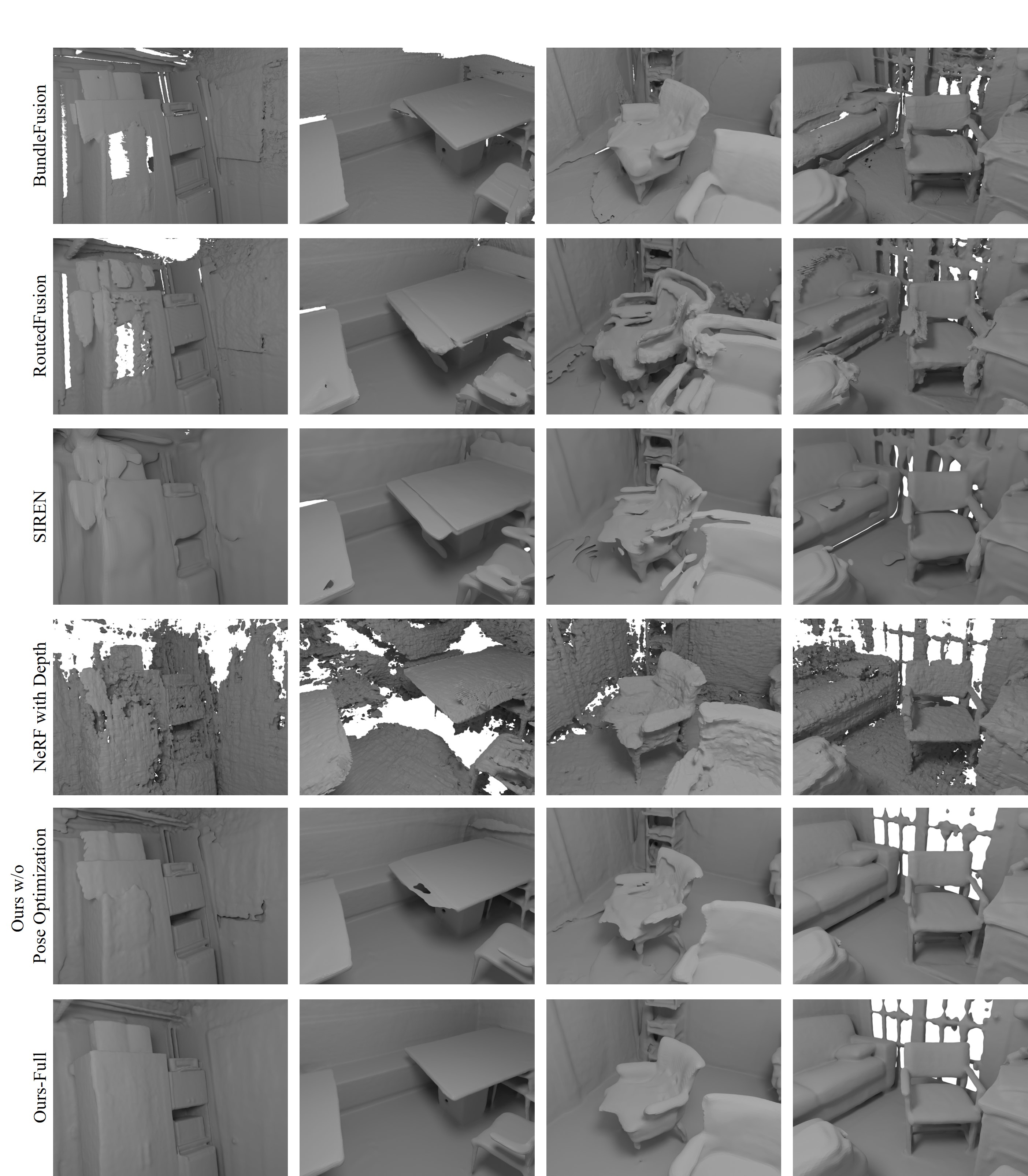
Figure 3: We compare our model without pose optimization and our full model with both the pose optimization and image-plane deformation field to BundleFusion, RoutedFusion, SIREN and a NeRF optimized with depth supervision in scenes 2, 5, 12, and 50 of the ScanNet dataset. Our model without pose optimization recovers smoother meshes than the density-based NeRF model, but still suffers from misalignment artifacts. These are solved by our full model to recover a clean reconstruction.

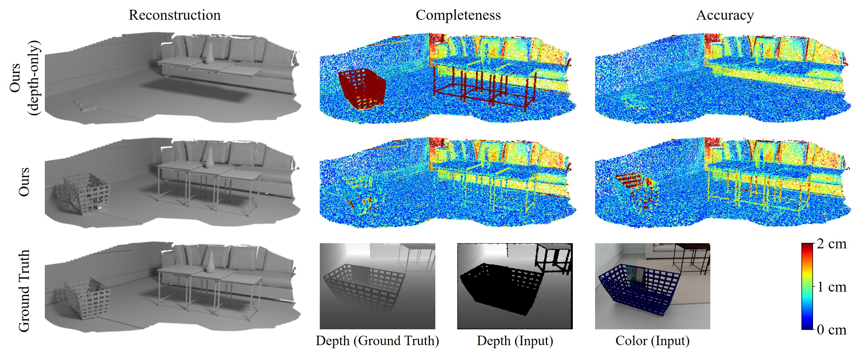
Figure 4: Accuracy shows how close ground truth points are to predicted points, while completeness shows how close predicted points are to ground truth points. Geometry reconstructed purely through the photometric loss has slightly lower accuracy than geometry for which depth observations were also available. Furthermore, the accuracy and completeness drop in distant areas, which had less multi-view constraints and more noise in the depth measurements.

Quantitative evaluation.

We perform a quantitative evaluation of our method on a dataset of 10 synthetic scenes for which the ground truth geometry and camera trajectory are known. Note that the ground truth camera trajectory is only used for the rendering and evaluation, and not for the reconstruction. For each frame, we render a photo-realistic image using Blender [8, 17]. We apply noise and artifacts, similar to those of a real depth sensor [30, 1, 3, 31]. On this data, we compare our technique to several state-of-the-art methods that use either depth input only, or both color and depth data to reconstruct geometry (see Tab. 1).

BundleFusion. BundleFusion [14] uses the color and depth input to reconstruct the scene. It is a classical depth fusion approach [9] which compensates misalignments using a global bundle adjustment approach.

RoutedFusion. RoutedFusion [79] uses a routing network which filters sensor-specific noise and outliers from depth maps and computes pixel-wise confidence values, which are used by a fusion network to produce the final SDF. It takes the depth maps and camera poses as input.

COLMAP with screened Poisson surface reconstruction. We obtain camera poses using COLMAP [63, 64, 65] and use these to back-project depth maps into world space. We obtain a mesh by applying screened Poisson surface reconstruction [35] on the resulting point cloud.

Convolutional Occupancy Networks. We accumulate the point clouds from the depth maps using BundleFusion poses and evaluate the pre-trained convolutional occupancy networks model [58] provided by the authors (which has been used on similar data [6]).

SIREN. We optimize a SIREN [67] per scene using the back-projected point cloud data. The ICL-NUIM [31] scene on which the method was originally tested, is also included in our synthetic dataset.

NeRF with an additional depth loss. NeRF [48] proposes using the expected ray termination distance as a way to visualize the depth of the scene. In our baseline, we add an additional loss to NeRF, where this depth value is compared to the input depth using an L2 loss. Note that this baseline still uses NeRF’s density field to represent geometry.

As can be seen in Tab. 1, our approach with camera refinement results in the lowest Chamfer distance, and the highest IoU, normal consistency (mean of the dot product of the ground truth and predicted normals), and F-score [37]. Especially, the comparison to the density-based NeRF with an additional depth constraint shows the benefit of our proposed hybrid scene representation.

Ablation studies.

We conduct ablation studies to justify our choice of network architecture and training parameters. In Fig. 3, we show the difference between a volumetric representation (density field, ‘NeRF with Depth’) to an implicit surface representation (signed distance field, ‘Ours-Full’) on real data from ScanNet [12]. While representing scenes with a density field works great for color integration, extracting the geometry itself is a challenging problem. Although small variations in density may not affect the integrated color much, they cause visible noise in the extracted geometry and produce floating artifacts in free space. These artifacts can be reduced by choosing a different iso-level for geometry extraction with Marching Cubes, but this leads to less complete reconstructions. In contrast, a signed distance field models a smooth boundary between occupied and free space, and we show that it can be faithfully represented by an MLP. However, the reconstruction quality is still limited by the provided camera poses, as can be seen in Fig. 3 (e.g., the cabinet in the left column). Optimizing for pose corrections further improves the quality of our reconstructions.

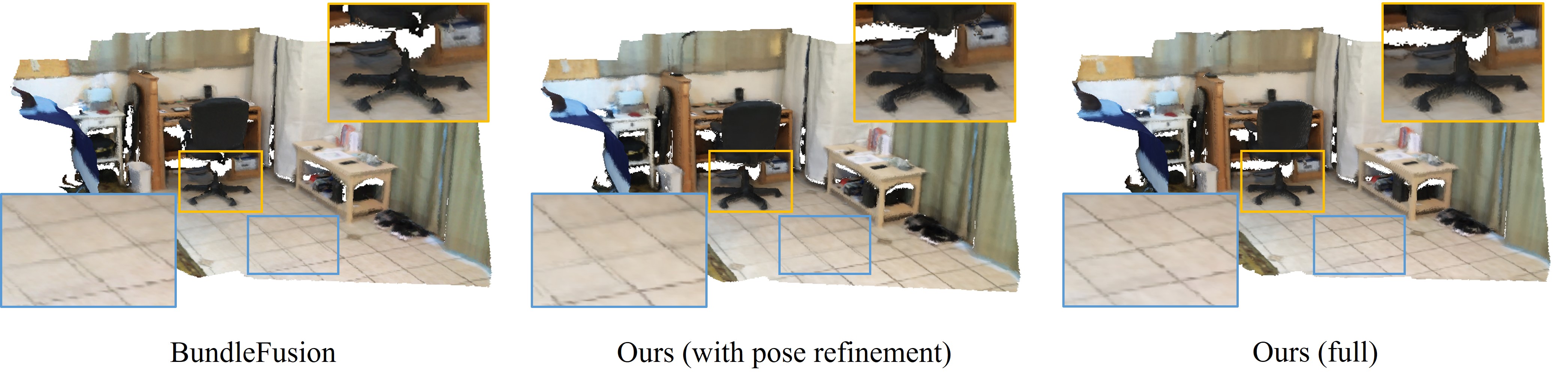
Figure 5: Our method improves the camera alignment over the baseline, as visible in the tiles of the floor. The additional image-plane distortion correction results in straight and aligned edges in the reconstruction.

Effect of the photometric term.

A fundamental component of our method is the use of a photometric term to infer depth values which are missing from camera measurements. We analyze the effect of this term on the synthetic scene in Fig. 4, where we simulate missing geometry of the table legs and the meshed basket. In the figure, we visualize the completeness and accuracy. In contrast to a model without the photometric term, our method is still able to reconstruct the missing geometry leveraging the RGB observations.

For our full approach, we also separately evaluate the reconstruction quality of geometry where depth measurements were available and where they were missing. Regions that relied only on color have a somewhat worse average accuracy of $11$ mm, compared to $8$ mm for regions that had access to depth measurements. We refer the reader to the supplemental material for more details and a qualitative comparison on real data.

Method	Pos. error (meters) $\downarrow$	Rot. error (degrees) $\downarrow$
BundleFusion	0.033	0.571
COLMAP	0.038	0.692
Ours	0.021	0.144

Table 2: Based on our synthetic dataset, we evaluate the average positional and rotational errors of the estimated camera poses. Our method is able to further increase the pose estimation accuracy compared to its BundleFusion initialization.

Effect of pose refinement.

We show that initial camera pose estimates can be further improved by jointly optimizing for the rotation and translation parameters of the cameras which are initialized with BundleFusion [14]. We quantitatively evaluate this on all scenes in our synthetic dataset. An aggregate of the positional and rotational errors of different methods is presented in Tab. 2. A detailed per-scene breakdown is given in the supplemental material. In Tab. 1 and Fig. 3, we show that optimizing camera poses reduces geometry misalignment artifacts and improves the overall reconstruction, both quantitatively and qualitatively.

Effect of the image-plane deformation field.

To evaluate the effect of the pixel-space deformation field, we initialize the camera with an incorrect focal length and optimize our model with and without the deformation field. Tab. 3 shows that the deformation field mitigates this inaccuracy in the camera’s intrinsic parameters which leads to significantly better reconstruction results compared to the model that does not use the deformation field. Fig. 5 showcases the effects of our camera pose and image-plane deformation field [14]. Blurry frames and sparse features lead to systematic camera pose errors in BundleFusion. Our method improves these camera poses and the camera distortion model, and, thus, is able to better align scene features, resulting in higher reconstruction quality.

Limitations and future work.

Similar to other methods that are based on a scene representation which uses a scene-specific MLP, our method runs offline (around $9$ hours for $2\times 10^{5}$ iterations using an NVIDIA RTX 3090). Recent methods that utilize voxel grids to optimize a radiance field [70, 86] have shown significantly faster convergence compared to earlier MLP-based methods and we believe that they would also be good candidates for improving our method. Nonetheless, our proposed method offers a high-quality scene reconstruction which outperforms online fusion approaches. Another limitation is the global MLP which stores the entire scene information which comes at the cost of missing high-frequency local detail in very large scenes. Approaches like IF-Nets [7] or Convolutional Occupancy Networks [58] benefit from locally-conditioned MLPs and can be integrated in future work. Finally, our method was designed to handle only opaque surfaces.

Method	C-$\ell_{1}$ $\downarrow$	IoU $\uparrow$	NC $\uparrow$	F-score $\uparrow$
Ours (w/o IPDF)	0.061	0.266	0.886	0.406
Ours (w/ IPDF)	0.031	0.609	0.911	0.904

Table 3: Ablation of the image-plane deformation field (IPDF) which compensates image space distortions and incorrect intrinsic parameters. The experiment is based on a synthetic scene, where we assume an incorrect focal length of $570$ instead of $554.26$ (GT).

5 Conclusion

We have presented a new method for 3D surface reconstruction from RGB-D sequences by introducing a hybrid scene representation that is based on an implicit surface function and a volumetric representation of radiance. This allows us to efficiently incorporate depth observations, while still benefiting from the differentiable volumetric rendering of the original neural radiance field formulation. As a result, we obtain high-quality surface reconstructions, outperforming traditional and learned RGB-D fusion methods. Overall, we believe our work is a stepping stone towards leveraging the success of implicit, differentiable representations for 3D surface reconstruction.

APPENDIX

In this appendix we show a per-scene breakdown of the quantitative evaluation from Tab. 1, an ablation study on additional scenes from the ScanNet dataset (see Fig. 6), as well as further ablation studies on synthetic data. For the purpose of reproducibility, we also provide further details on the parameters that were used for optimization in each of the scenes.

Appendix A Implementation Details

We implement our method in TensorFlow v2.4.1 using the ADAM [36] optimizer with a learning rate of $5\times 10^{-4}$ and an exponential learning rate decay of $10^{-1}$ over $2.5\times 10^{5}$ iterations. In each iteration, we compute a gradient w.r.t. $|P_{b}|=1024$ randomly chosen rays. We set the number of $S^{\prime}_{f}$ samples to 16. $S^{\prime}_{c}$ is chosen so that there is on average one sample for every 1.5 cm of the ray length. Tab. 4 gives an overview of ray length and number of samples for each of the experiments. Internally, we translate and scale each scene so that it lies within a $[-1,1]^{3}$ cube. Depending on scene size, our method takes between $9$ and $13$ hours to converge on a single NVIDIA RTX 3090 (see Sec. F). We set the loss weights to $\lambda_{1}=0.1$, $\lambda_{2}=10$ and $\lambda_{3}=6\times 10^{3}$. We use $8$ bands for the positional encoding of the point coordinates and $4$ bands to encode the view direction vector.

To account for distortions or inaccuracies of the intrinsic parameters, a 2D deformation field of the camera pixel space in form of a 6-layer MLP, with a width of 128, is used.

Scene	$S^{\prime}_{c}$	$ray$ $length$ (m)	$\#frames$
Scene 0	512	8	1394
Scene 2	256	4	1299
Scene 5	256	4	1159
Scene 12	320	5	1335
Scene 24	512	8	849
Scene 50	256	4	1163
Scene 54	256	4	1250
Breakfast room	320	5	1167
Green room	512	8	1442
Grey-white room	512	8	1493
ICL living room	320	5	1510
Kitchen 1	512	8	1517
Kitchen 2	640	10	1221
Morning apartment	256	4	920
Staircase	512	8	1149
Thin geometry	256	4	395
White room	512	8	1676

Table 4: We list the number of samples $S^{\prime}_{c}$ and the ray length in meters that were used to reconstruct each of the ScanNet scenes and the synthetic scenes. Note that these settings are dependent on the scene size.

Appendix B Per-scene Quantitative Evaluations

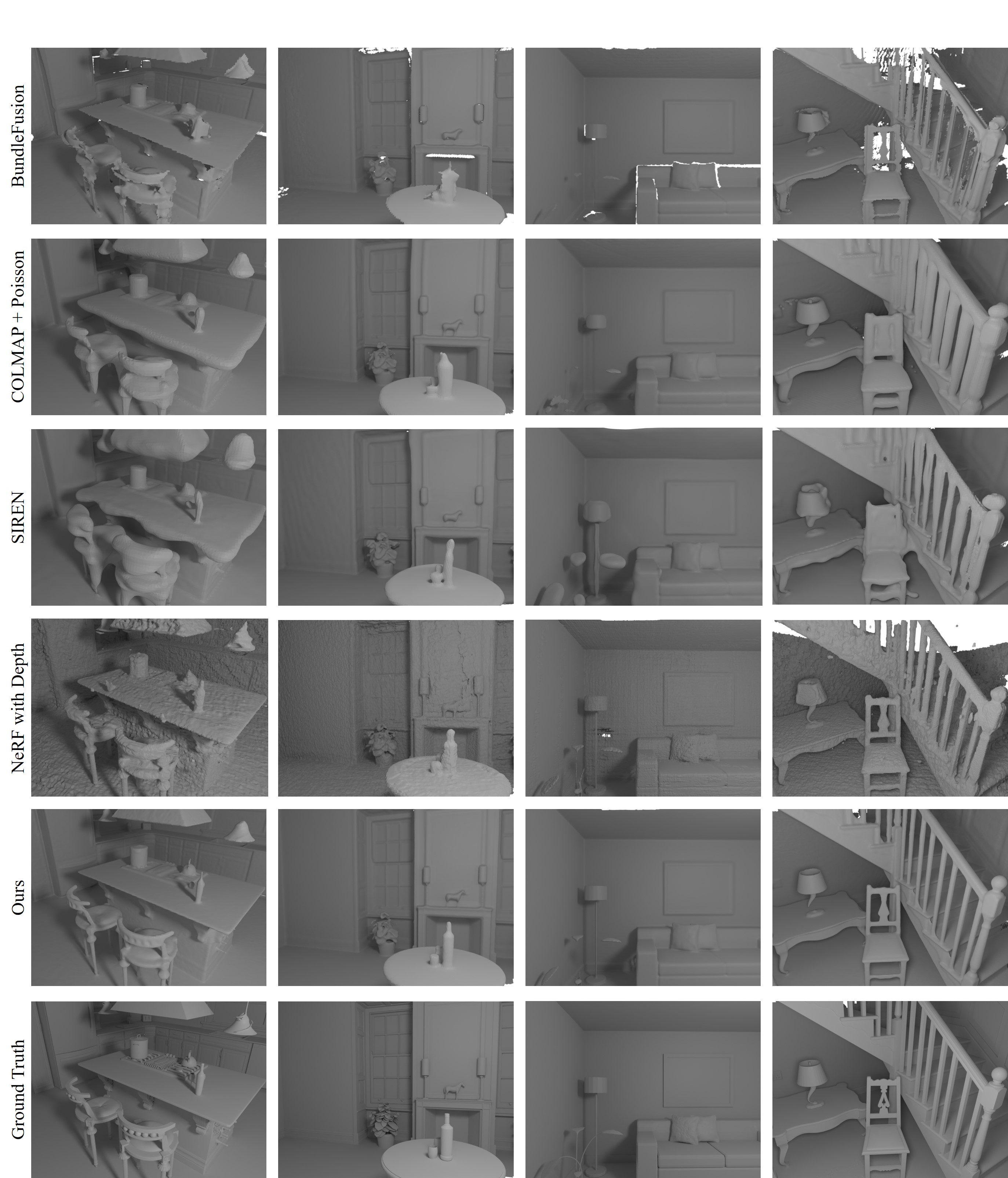
Figure 14: We show a qualitative comparison of synthetic scene reconstructions obtained using our method and several baseline methods. The BundleFusion reconstruction is incomplete in some regions, screened Poisson and SIREN attempt to fit noise in the depth data, while the NeRF reconstruction suffers from noise in the density field. Our method manages to fill in gaps in geometry, while maintaining the smoothness of classic fusion approaches.

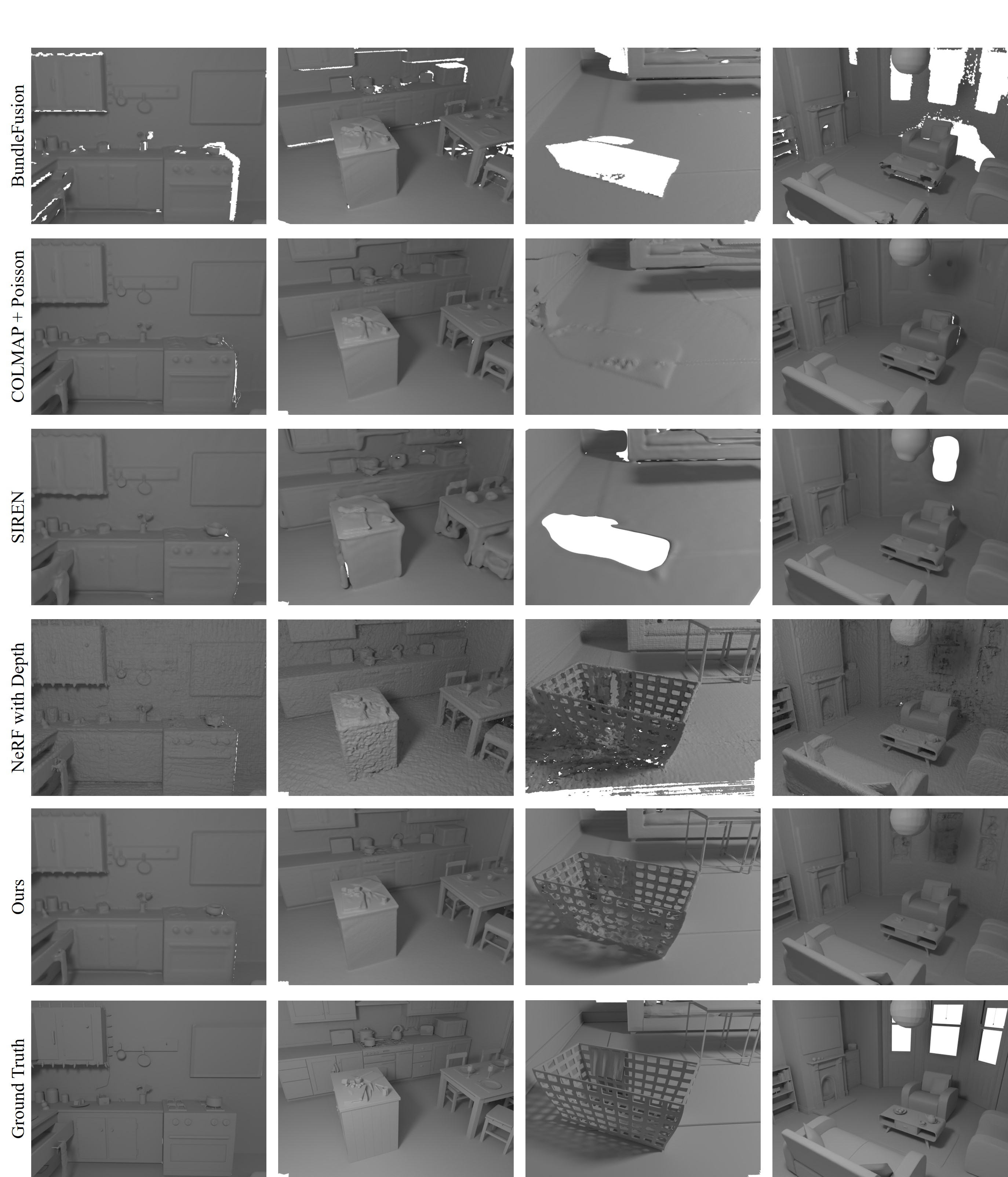
Figure 15: We show a qualitative comparison of synthetic scene reconstructions obtained using our method and several baseline methods. The BundleFusion reconstruction is incomplete in some regions, screened Poisson and SIREN attempt to fit noise in the depth data, while the NeRF reconstruction suffers from noise in the density field. Our method manages to fill in gaps in geometry, while maintaining the smoothness of classic fusion approaches.

In Tab. LABEL:tab:quantitative_per_scene_1 and Tab. LABEL:tab:quantitative_per_scene_2 we present a per-scene breakdown of the quantitative analysis from the main paper (see Sec. 4, Tab. 1 and Tab. 2 in the main paper). The corresponding qualitative results are shown in Fig. 14 and Fig. 15.

Reconstruction Evaluation.

The goal of our method is to reconstruct a scene from color and depth data, i.e., we do not aim for scene completion. To evaluate the reconstruction quality, we evaluate the quality of reconstructions w.r.t. Chamfer distance (C-$\ell_{1}$), intersection-over-union (IoU), normal consistency (NC) based on cosine similarity, and F-score. These metrics are computed on surfaces which were visible in the color and depth streams (geometry within the viewing frusta of the input images). Specifically, we subdivide all meshes to have a maximum edge length of below $1.5$ cm and use the ground truth trajectory to detect vertices which are visible in at least one camera. Triangles which have no visible vertices, either due to not being in any of the viewing frusta or due to being occluded by other geometry, are culled. This is necessary to avoid computing the error in regions such as occluded geometry in the synthetic ground truth mesh or in regions where the network output is unpredictable because the region was never seen at training time. The culled geometry is sampled with a density of 1 point per cm² and the error metrics are evaluated on the sampled point clouds. To evaluate the IoU, we voxelize the reconstruction using voxels with an edge length of $5$ cm. The F-score is also computed using a $5$ cm threshold.

Synthetic Dataset.

Our synthetic dataset which we use for numeric evaluation purposes consists of 10 scenes published under either the CC-BY or CC-0 license (see Tab. 5). We define a trajectory by a Catmull-Rom spline interpolation [88] on several manually chosen control points. We use BlenderProc [17] to render color and depth images for each camera pose in the interpolated trajectory. Noise is applied to the depth maps to simulate sensor noise of a real depth sensor [30, 1, 3, 31]. For the ICL scene [31], we use the color and noisy depth provided by the authors and do not render our own images. The scenes in the dataset have various sizes, complexity and materials like highly specular surfaces or mirrors. BundleFusion [14] is used to get an initial estimate of the camera trajectory. This estimated trajectory is used by all methods other than COLMAP to allow a fair comparison.

Scene	URL	License
ScanNet	http://www.scan-net.org/	MIT
Breakfast room	https://blendswap.com/blend/13363	CC-BY
Green room	https://blendswap.com/blend/8381	CC-BY
Grey-white room	https://blendswap.com/blend/13552	CC-BY
ICL living room	https://www.doc.ic.ac.uk/ ahanda/VaFRIC/iclnuim.html	CC-BY
Kitchen 1	https://blendswap.com/blend/5156	CC-BY
Kitchen 2	https://blendswap.com/blend/11801	CC-0
Morning apart.	https://blendswap.com/blend/10350	CC-0
Staircase	https://blendswap.com/blend/14449	CC-BY
Thin geometry	https://blendswap.com/blend/8381	CC-BY
White room	https://blendswap.com/blend/5014	CC-BY

Table 5: Source and license information of the used data.

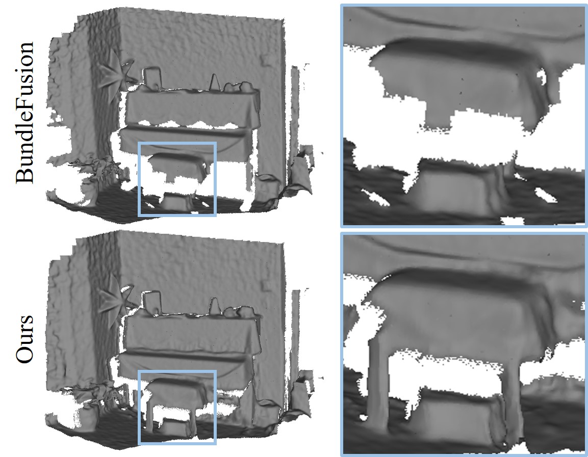
Figure 7: The photometric energy term encourages correct depth prediction in areas where the depth sensor did not capture any depth measurements.

Appendix C Ablation Studies

In this section, we present additional details for the ablation studies described in the main paper, and show further studies to test the robustness and the limitations of our method. In Fig. 6, the additional results on real data demonstrate the advantages of the signed distance field and our camera refinement.

Method	C-$\ell_{1}$ $\downarrow$	IoU $\uparrow$	NC $\uparrow$	F-score $\uparrow$
Ours (depth-only)	0.017	0.791	0.910	0.944
Ours (full)	0.009	0.865	0.910	0.995

Table 6: Detailed reconstruction results for Fig. 4 from the main paper. Our method reconstructs geometry visible only in color images, leading to significantly better reconstruction results in scenes with geometry which is not captured by the depth sensor.

C.1 Effect of the Photometric Energy Term

In Tab. 6, we list the quantitative evaluation of the experiment on the effectiveness of the photometric energy term from Fig. 4 in the main paper. Fig. 7 shows the effect of the term on a real scene from the ScanNet dataset. The legs of the piano stool were not visible in any of the depth maps. Nevertheless, our method is able to reconstruct them by making use of the corresponding color data.

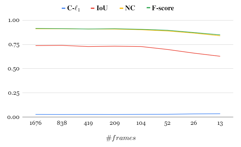
Figure 8: We test the robustness of our method by removing frames from the dataset used for optimization. Our method achieves good reconstruction results using as few as 13 frames.

C.2 Number of Input Frames

The reconstruction quality of any reconstruction method is dependent on the number of input frames. We evaluate our method on the ‘whiteroom’ synthetic scene through multiple experiments in which we remove different numbers of frames in the dataset used for optimization. Reconstruction results are presented in Fig. 8. Note that for these experiments we use the camera poses initialized with BundleFusion which uses all $1676$ depth frames.

C.3 Robustness to Noisy Pose Initialization

To analyze the robustness of our method w.r.t. presence of inaccuracies in camera alignment, we apply Gaussian noise to every camera’s position and direction in the ‘whiteroom’ scene. In Fig. 9 we present reconstruction results for poses of increasing inaccuracy. We separately show the pose errors of the refined cameras in Fig. 10. On the reconstruction metrics, our method is robust to camera position and orientation errors of up to $5$ cm and $5^{\circ}$ respectively. The pose refinement is robust up to a noise level of $3$ cm and $3^{\circ}$. At noise levels with a standard deviation of $10$ cm and higher, some cameras are initially positioned inside geometry, preventing our method from refining their position and leading to large errors in geometry reconstruction.

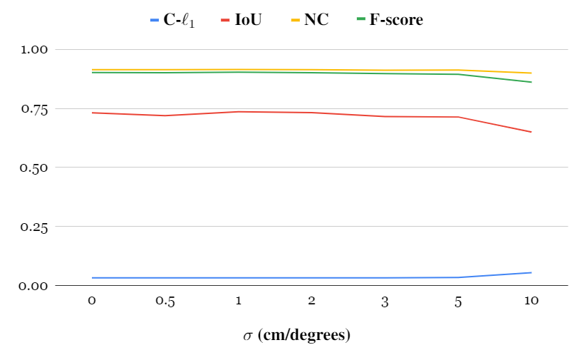
Figure 9: We test the robustness of our reconstructions to noise in the initial camera position and direction. Our method achieves good results even in the presence of significant noise. At $\sigma$ = $10$ cm, some of the cameras intersect geometry, degrading the reconstruction quality.

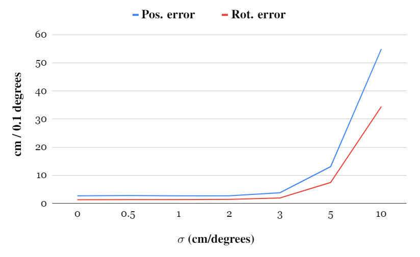
Figure 10: We test the robustness of our pose refinement to noise in the initial camera position and direction. The rotation error has been scaled by a factor of $10$ for better visibility. Our method is able to correct poses even in the presence of significant noise. At $\sigma$ = $10$ cm, some of the cameras start intersecting geometry, making refinement impossible.

Truncation (cm)	C-$\ell_{1}$ $\downarrow$	IoU $\uparrow$	NC $\uparrow$	F-score $\uparrow$
2	0.053	0.671	0.855	0.862
3	0.023	0.766	0.901	0.930
5	0.021	0.786	0.912	0.933
10	0.024	0.742	0.908	0.912

Table 7: Impact of the truncation region width on reconstruction quality.

C.4 Batch Size

Optimization with a lower batch size leads to more noise and might miss areas without depth supervision due to a lower number of multi-view constraints within the batch. A batch size that is too large will slow down the optimization and consume more GPU memory, while not offering improvements in reconstruction quality (see Fig. 11).

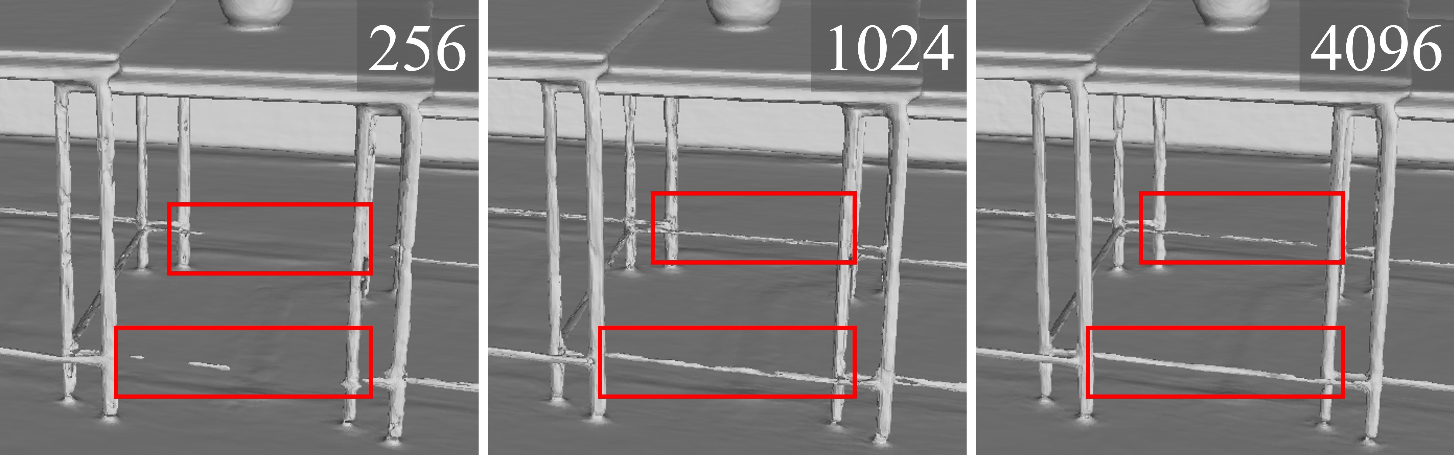
Figure 11: Reconstruction quality with varying batch size.

C.5 Truncation Size

The reconstruction quality is dependent on the width of the truncation region, as shown in Tab. 7. The truncation region needs to account for the noise in the input (i.e., needs to be greater than the noise of the depth camera). In our experiments a truncation radius of $tr=5$ cm gives the best results (evaluated based on the mean across multiple scenes).

Appendix D Comparison to RGB-based methods

NeuS [76] and VolSDF [83] are concurrent works that propose learning a signed distance field of an object from a set of RGB images. In contrast to these methods, our focus lies on reconstructing indoor scenes which often have large textureless regions (e.g., a white wall). Methods which use only color input will not have enough multi-view constraints to properly reconstruct these regions. In Fig. 12, we show a case where methods that rely only on color input struggle to reconstruct high-quality geometry.

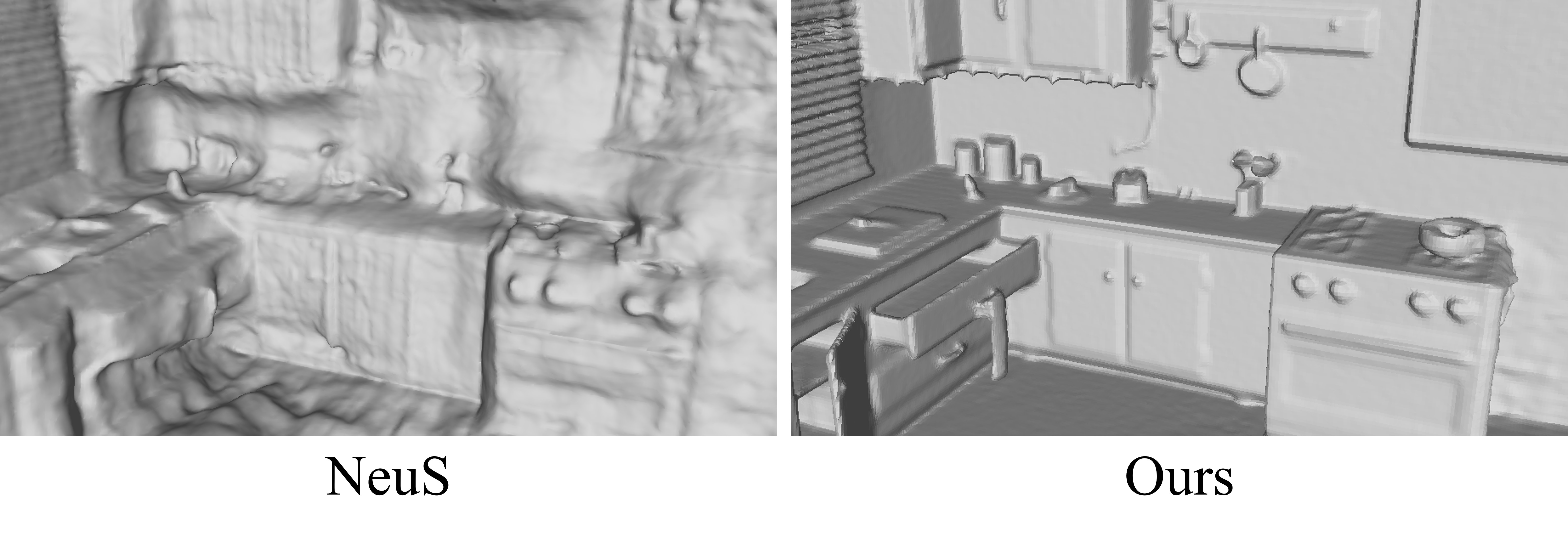
Figure 12: Comparison between NeuS and our method on the ‘morning apartment’ scene.

Appendix E Color Reproduction of Classic and NeRF-style Methods

While our focus lies on geometry reconstruction and not accurate view synthesis, we conducted a brief analysis of the advantages and drawbacks of classic reconstruction methods [14, 92] and MLP-based radiance fields [48] when synthesizing unseen views. Classic reconstruction methods usually do not try to decouple intrinsic material parameters [14, 92] and instead optimize a texture that represents the average observation of all the input views. The resulting texture is usually high-resolution (bounded by the resolution of the input images), but does not allow for correct synthesis of view-dependent effects. Furthermore, inaccuracies in camera calibration may lead to visible seams in the optimized texture. Methods like NeRF that focus purely on high-quality novel view synthesis do not explicitly reconstruct geometry and may thus produce images riddled with artifacts for views that are too far from the input views. We believe that it is possible to combine both of these approaches to improve novel view synthesis on views far away from the ones used during the optimization and would like to encourage research in this direction. Fig. 13 shows an example view synthesis result on the ScanNet dataset, for an out-of-trajectory camera position and orientation.

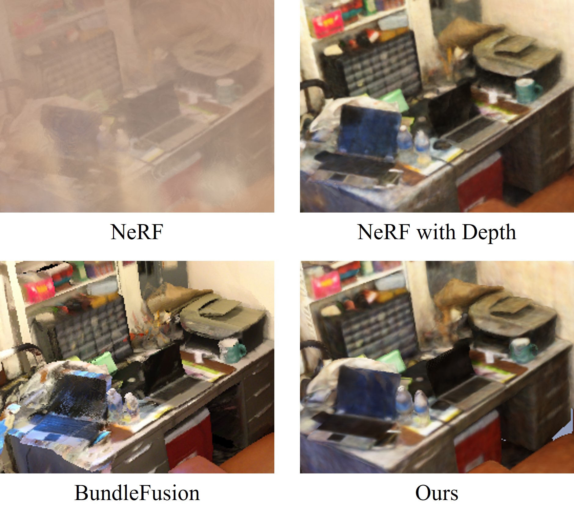
Figure 13: We compare the color synthesis of BundleFusion and NeRF-style methods. NeRF without any depth constraints shows severe fogging when rendering an image from a novel view. This gets resolved after adding depth constraints to the optimization. BundleFusion produces the sharpest results, but suffers from incorrect view-dependent effects and misalignment artifacts. Our method produces results similar to NeRF with a depth constraint. A combination of classic and NeRF-style methods may yield both high-quality geometry and high-quality view synthesis and we encourage further research in this direction.

Appendix F Runtime and Memory Requirements

Our method.

The runtime and memory requirements of our method are dependent on the scene size. For smaller scenes where it is enough to have $S^{\prime}_{c}=256$ samples, our method completes $2\times 10^{5}$ iterations in $9$ hours on an NVIDIA RTX 3090 and requires $8.5$ GB of GPU memory. When $S^{\prime}_{c}$ is set to 512, the runtime increases to $13$ hours and the memory requirement to $10.5$ GB. The memory consumption can be reduced by using smaller batches.

BundleFusion.

We run BundleFusion at a voxel resolution of $1$ cm for all scenes. On an NVIDIA GTX TITAN Black, depending on the size of the scene and number of frames in the camera trajectory, it takes $10$ to $40$ minutes to integrate the depth frames into a truncated signed distance field and extract a mesh using Marching Cubes. The memory usage is around $5.8$ GB.

RoutedFusion.

To train and test RoutedFusion, we used an NVIDIA RTX 3090. The routing network was trained for 24 hours on images with a resolution of $320\times 240$ pixels. As per suggestion of the authors, we train the fusion network for $20$ epochs which takes about $1.5$ hours. We reconstruct all scenes at a voxel resolution of $1$ cm for a fair comparison to other methods. The runtime ranges from $40$ minutes to $6$ hours depending on scene size and number of frames. The memory usage also heavily depends on scene size and ranges from $5.5$ GB to $23$ GB.

COLMAP + Poisson.

In the COLMAP + Poisson baseline, the bottleneck is the global bundle adjustment process performed by COLMAP. The total runtime depends on the number of frames in the trajectory. Using all 8 cores of an Intel i7-7700K CPU, it took us about $4$ hours to align all 1167 cameras in the ‘breakfast room’. The couple of minutes needed to backproject all depth maps at full resolution and run the screened Poisson surface reconstruction are negligible in comparison.

Convolutional Occupancy Networks.

We reconstruct each scene using the pre-trained model provided by the authors. This takes about $2$ minutes per scene and requires about $10$ GB of memory.

SIREN.

We train SIREN for $10^{4}$ epochs on each scene. SIREN is trained over the complete point cloud in each epoch, so the runtime depends on the number of points in the point cloud. In our experiments on an NVIDIA RTX 3090, this ranged from $6$ to $12$ hours with $12$ GB of memory being in use.

NeRF + Depth.

We optimize NeRF using 64 samples for the coarse network and 128 samples for the fine network. On an NVIDIA RTX 3090 it takes $6$ hours for $2\times 10^{5}$ iterations to run. The memory usage is $4.7$ GB.

Table 8: We compare the quality of our reconstruction on several synthetic scenes for which ground truth data is available. The Chamfer $\ell_{1}$ distance, normal consistency and the F-score [37] are computed between point clouds sampled with a density of 1 point per cm². We use a threshold of 5 cm for the F-score. We further voxelize each mesh to compute the intersection-over-union (IoU) between the predictions and ground truth.

Scene	Method	C-$\ell_{1}$ $\downarrow$	IoU $\uparrow$	NC $\uparrow$	F-score $\uparrow$	Pos. error $\downarrow$	Rot. error $\downarrow$
Breakfast room	BundleFusion	0.033	0.698	0.944	0.890	0.037	0.697
	RoutedFusion	0.033	0.714	0.918	0.901	-	-
	COLMAP + Poisson	0.033	0.668	0.935	0.893	0.009	0.210
	Conv. Occ. Nets	0.047	0.474	0.879	0.780	-	-
	SIREN	0.060	0.566	0.922	0.822	-	-
	NeRF + Depth	0.041	0.619	0.811	0.854	-	-
	Ours (w/o pose)	0.031	0.720	0.930	0.914	-	-
	Ours	0.030	0.793	0.934	0.920	0.007	0.135
Green room	BundleFusion	0.024	0.694	0.923	0.926	0.027	0.546
	RoutedFusion	0.018	0.755	0.904	0.969	-	-
	COLMAP + Poisson	0.018	0.849	0.925	0.967	0.014	0.227
	Conv. Occ. Nets	0.053	0.554	0.855	0.737	-	-
	SIREN	0.023	0.746	0.913	0.940	-	-
	NeRF + Depth	0.030	0.668	0.748	0.871	-	-
	Ours (w/o pose)	0.014	0.766	0.931	0.982	-	-
	Ours	0.013	0.921	0.932	0.990	0.012	0.104
Grey-white room	BundleFusion	0.038	0.567	0.860	0.751	0.056	1.891
	RoutedFusion	0.033	0.606	0.850	0.790	-	-
	COLMAP + Poisson	0.029	0.727	0.899	0.899	0.029	0.296
	Conv. Occ. Nets	0.048	0.480	0.841	0.601	-	-
	SIREN	0.033	0.635	0.868	0.812	-	-
	NeRF + Depth	0.040	0.563	0.764	0.697	-	-
	Ours (w/o pose)	0.032	0.640	0.864	0.806	-	-
	Ours	0.015	0.886	0.924	0.987	0.014	0.146
ICL living room	BundleFusion	0.018	0.743	0.956	0.958	0.022	0.382
	RoutedFusion	0.019	0.698	0.939	0.976	-	-
	COLMAP + Poisson	0.023	0.727	0.947	0.966	0.029	0.836
	Conv. Occ. Nets	0.112	0.352	0.841	0.507	-	-
	SIREN	0.020	0.768	0.950	0.967	-	-
	NeRF + Depth	0.021	0.689	0.900	0.956	-	-
	Ours (w/o pose)	0.014	0.790	0.964	0.992	-	-
	Ours	0.011	0.905	0.969	0.994	0.007	0.109
Kitchen 1	BundleFusion	0.234	0.368	0.860	0.620	0.038	0.327
	RoutedFusion	0.265	0.401	0.805	0.680	-	-
	COLMAP + Poisson	0.252	0.459	0.888	0.748	0.103	0.941
	Conv. Occ. Nets	0.262	0.352	0.839	0.483	-	-
	SIREN	0.265	0.357	0.850	0.575	-	-
	NeRF + Depth	0.271	0.336	0.710	0.600	-	-
	Ours (w/o pose)	0.255	0.420	0.887	0.700	-	-
	Ours	0.252	0.447	0.886	0.718	0.030	0.114

Table 9: We compare the quality of our reconstruction on several synthetic scenes for which ground truth data is available. The Chamfer $\ell_{1}$ distance, normal consistency and the F-score [37] are computed between point clouds sampled with a density of 1 point per cm². We use a threshold of 5 cm for the F-score. We further voxelize each mesh to compute the intersection-over-union (IoU) between the predictions and ground truth.

Scene	Method	C-$\ell_{1}$ $\downarrow$	IoU $\uparrow$	NC $\uparrow$	F-score $\uparrow$	Pos. error $\downarrow$	Rot. error $\downarrow$
Kitchen 2	BundleFusion	0.089	0.441	0.856	0.687	0.050	0.566
	RoutedFusion	0.059	0.572	0.842	0.787	-	-
	COLMAP + Poisson	0.037	0.675	0.919	0.818	0.043	1.154
	Conv. Occ. Nets	0.052	0.484	0.861	0.653	-	-
	SIREN	0.055	0.453	0.898	0.735	-	-
	NeRF + Depth	0.051	0.435	0.708	0.630	-	-
	Ours (w/o pose)	0.034	0.488	0.908	0.796	-	-
	Ours	0.032	0.637	0.903	0.890	0.083	0.450
Morning apartment	BundleFusion	0.012	0.767	0.885	0.968	0.008	0.165
	RoutedFusion	0.013	0.815	0.870	0.976	-	-
	COLMAP + Poisson	0.017	0.668	0.877	0.959	0.017	0.380
	Conv. Occ. Nets	0.045	0.450	0.802	0.784	-	-
	SIREN	0.013	0.727	0.873	0.966	-	-
	NeRF + Depth	0.022	0.587	0.838	0.975	-	-
	Ours (w/o pose)	0.011	0.787	0.887	0.983	-	-
	Ours	0.011	0.716	0.888	0.982	0.005	0.093
Staircase	BundleFusion	0.091	0.373	0.860	0.623	0.039	0.643
	RoutedFusion	0.069	0.340	0.864	0.622	-	-
	COLMAP + Poisson	0.074	0.322	0.895	0.628	0.043	0.305
	Conv. Occ. Nets	0.069	0.315	0.838	0.508	-	-
	SIREN	0.067	0.432	0.885	0.676	-	-
	NeRF + Depth	0.087	0.396	0.644	0.624	-	-
	Ours (w/o pose)	0.057	0.457	0.899	0.704	-	-
	Ours	0.045	0.565	0.920	0.853	0.016	0.123
Thin geometry	BundleFusion	0.019	0.764	0.909	0.922	0.009	0.126
	RoutedFusion	0.023	0.708	0.829	0.881	-	-
	COLMAP + Poisson	0.047	0.440	0.820	0.721	0.079	2.400
	Conv. Occ. Nets	0.022	0.723	0.882	0.910	-	-
	SIREN	0.021	0.733	0.887	0.913	-	-
	NeRF + Depth	0.014	0.825	0.847	0.989	-	-
	Ours (w/o pose)	0.009	0.857	0.911	0.995	-	-
	Ours	0.009	0.865	0.910	0.995	0.010	0.037
White room	BundleFusion	0.062	0.528	0.869	0.701	0.045	0.375
	RoutedFusion	0.038	0.545	0.817	0.799	-	-
	COLMAP + Poisson	0.036	0.652	0.904	0.796	0.018	0.167
	Conv. Occ. Nets	0.061	0.424	0.853	0.470	-	-
	SIREN	0.046	0.617	0.888	0.752	-	-
	NeRF + Depth	0.073	0.385	0.716	0.619	-	-
	Ours (w/o pose)	0.034	0.631	0.902	0.813	-	-
	Ours	0.028	0.738	0.911	0.915	0.028	0.133

References

- [1] Jonathan T. Barron and Jitendra Malik. Intrinsic scene properties from a single rgb-d image. CVPR, 2013.
- [2] Michael Bloesch, Jan Czarnowski, Ronald Clark, Stefan Leutenegger, and Andrew J. Davison. Codeslam — learning a compact, optimisable representation for dense visual slam. In Proceedings of the IEEE Conference on Computer Vision and Pattern Recognition (CVPR), June 2018.
- [3] Jeannette Bohg, Javier Romero, Alexander Herzog, and Stefan Schaal. Robot arm pose estimation through pixel-wise part classification. ICRA, 2014.
- [4] Aljaž Božič, Pablo Palafox, Justus Thies, Angela Dai, and Matthias Nießner. Transformerfusion: Monocular rgb scene reconstruction using transformers. Proc. Neural Information Processing Systems (NeurIPS), 2021.
- [5] Eric Chan, Marco Monteiro, Petr Kellnhofer, Jiajun Wu, and Gordon Wetzstein. pi-gan: Periodic implicit generative adversarial networks for 3d-aware image synthesis. In arXiv, 2020.
- [6] Angel Chang, Angela Dai, Thomas Funkhouser, Maciej Halber, Matthias Niessner, Manolis Savva, Shuran Song, Andy Zeng, and Yinda Zhang. Matterport3d: Learning from rgb-d data in indoor environments. International Conference on 3D Vision (3DV), 2017.
- [7] Julian Chibane, Thiemo Alldieck, and Gerard Pons-Moll. Implicit functions in feature space for 3d shape reconstruction and completion. In IEEE Conference on Computer Vision and Pattern Recognition (CVPR). IEEE, jun 2020.
- [8] Blender Online Community. Blender - a 3D modelling and rendering package. Blender Foundation, Stichting Blender Foundation, Amsterdam, 2018.
- [9] Brian Curless and Marc Levoy. A volumetric method for building complex models from range images. In Proceedings of the 23rd Annual Conference on Computer Graphics and Interactive Techniques, SIGGRAPH ’96, page 303–312, New York, NY, USA, 1996. Association for Computing Machinery.
- [10] J Czarnowski, T Laidlow, R Clark, and AJ Davison. Deepfactors: Real-time probabilistic dense monocular slam. IEEE Robotics and Automation Letters, 5:721–728, 2020.
- [11] Manuel Dahnert, Ji Hou, Matthias Nießner, and Angela Dai. Panoptic 3D scene reconstruction from a single RGB image. 2021.
- [12] Angela Dai, Angel X. Chang, Manolis Savva, Maciej Halber, Thomas Funkhouser, and Matthias Nießner. Scannet: Richly-annotated 3d reconstructions of indoor scenes. In Proc. Computer Vision and Pattern Recognition (CVPR), IEEE, 2017.
- [13] Angela Dai, Christian Diller, and Matthias Nießner. Sg-nn: Sparse generative neural networks for self-supervised scene completion of rgb-d scans. In Proc. Computer Vision and Pattern Recognition (CVPR), IEEE, 2020.
- [14] Angela Dai, Matthias Nießner, Michael Zollhöfer, Shahram Izadi, and Christian Theobalt. Bundlefusion: Real-time globally consistent 3d reconstruction using on-the-fly surface reintegration. ACM Transactions on Graphics (TOG), 36(4):76a, 2017.
- [15] Angela Dai, Yawar Siddiqui, Justus Thies, Julien Valentin, and Matthias Nießner. Spsg: Self-supervised photometric scene generation from rgb-d scans. In Proc. Computer Vision and Pattern Recognition (CVPR), IEEE, 2021.
- [16] Kangle Deng, Andrew Liu, Jun-Yan Zhu, and Deva Ramanan. Depth-supervised nerf: Fewer views and faster training for free. arXiv preprint arXiv:2107.02791, 2021.
- [17] Maximilian Denninger, Martin Sundermeyer, Dominik Winkelbauer, Youssef Zidan, Dmitry Olefir, Mohamad Elbadrawy, Ahsan Lodhi, and Harinandan Katam. Blenderproc. arXiv preprint arXiv:1911.01911, 2019.
- [18] Maximilian Denninger and Rudolph Triebel. 3d scene reconstruction from a single viewport. In Proceedings of the European Conference on Computer Vision (ECCV), 2020.
- [19] Wei Dong, Qiuyuan Wang, Xin Wang, and Hongbin Zha. PSDF fusion: Probabilistic signed distance function for on-the-fly 3d data fusion and scene reconstruction. CoRR, abs/1807.11034, 2018.
- [20] J. Engel, T. Schöps, and D. Cremers. LSD-SLAM: Large-scale direct monocular SLAM. In European Conference on Computer Vision (ECCV), September 2014.
- [21] J. Engel, J. Sturm, and D. Cremers. Semi-dense visual odometry for a monocular camera. In 2013 IEEE International Conference on Computer Vision, pages 1449–1456, 2013.
- [22] John Flynn, Ivan Neulander, James Philbin, and Noah Snavely. Deepstereo: Learning to predict new views from the world’s imagery. In Proceedings of the IEEE conference on computer vision and pattern recognition, pages 5515–5524, 2016.
- [23] C. Forster, M. Pizzoli, and D. Scaramuzza. Svo: Fast semi-direct monocular visual odometry. In 2014 IEEE International Conference on Robotics and Automation (ICRA), pages 15–22, 2014.
- [24] Huan Fu, Mingming Gong, Chaohui Wang, Kayhan Batmanghelich, and Dacheng Tao. Deep ordinal regression network for monocular depth estimation. In Proceedings of the IEEE Conference on Computer Vision and Pattern Recognition, pages 2002–2011, 2018.
- [25] Y. Furukawa and J. Ponce. Accurate, dense, and robust multiview stereopsis. IEEE Transactions on Pattern Analysis and Machine Intelligence, 32(8):1362–1376, 2010.
- [26] Guy Gafni, Justus Thies, Michael Zollhöfer, and Matthias Nießner. Dynamic neural radiance fields for monocular 4d facial avatar reconstruction. In Proceedings of the IEEE Conference on Computer Vision and Pattern Recognition, 2021.
- [27] Georgia Gkioxari, Jitendra Malik, and Justin Johnson. Mesh R-CNN. CoRR, abs/1906.02739, 2019.
- [28] Clément Godard, Oisin Mac Aodha, and Gabriel J Brostow. Unsupervised monocular depth estimation with left-right consistency. In Proceedings of the IEEE Conference on Computer Vision and Pattern Recognition, pages 270–279, 2017.
- [29] M. Goesele, N. Snavely, B. Curless, H. Hoppe, and S. M. Seitz. Multi-view stereo for community photo collections. In 2007 IEEE 11th International Conference on Computer Vision, pages 1–8, 2007.
- [30] Ankur Handa. Simulating kinect noise for the icl-nuim dataset. https://github.com/ankurhanda/simkinect. Accessed: 2021-11-15.
- [31] Ankur Handa, Thomas Whelan, John McDonald, and Andrew J Davison. A benchmark for rgb-d visual odometry, 3d reconstruction and slam. ICRA, 2014.
- [32] Vu Hoang Hiep, Renaud Keriven, Patrick Labatut, and Jean-Philippe Pons. Towards high-resolution large-scale multi-view stereo. In 2009 IEEE Conference on Computer Vision and Pattern Recognition, pages 1430–1437. IEEE, 2009.
- [33] Shahram Izadi, David Kim, Otmar Hilliges, David Molyneaux, Richard Newcombe, Pushmeet Kohli, Jamie Shotton, Steve Hodges, Dustin Freeman, Andrew Davison, et al. Kinectfusion: real-time 3d reconstruction and interaction using a moving depth camera. In Proceedings of the 24th annual ACM symposium on User interface software and technology, pages 559–568. ACM, 2011.
- [34] Abhishek Kar, Christian Häne, and Jitendra Malik. Learning a multi-view stereo machine. arXiv preprint arXiv:1708.05375, 2017.
- [35] Michael Kazhdan and Hugues Hoppe. Screened poisson surface reconstruction. ACM Trans. Graph., 32(3), July 2013.
- [36] Diederik P. Kingma and Jimmy Ba. Adam: A method for stochastic optimization. CoRR, abs/1412.6980, 2014.
- [37] Arno Knapitsch, Jaesik Park, Qian-Yi Zhou, and Vladlen Koltun. Tanks and temples: Benchmarking large-scale scene reconstruction. ACM Trans. Graph., 36(4), July 2017.
- [38] Kiriakos N Kutulakos and Steven M Seitz. A theory of shape by space carving. International journal of computer vision, 38(3):199–218, 2000.
- [39] Iro Laina, Christian Rupprecht, Vasileios Belagiannis, Federico Tombari, and Nassir Navab. Deeper depth prediction with fully convolutional residual networks. In 2016 Fourth international conference on 3D vision (3DV), pages 239–248. IEEE, 2016.
- [40] Zhengqi Li, Simon Niklaus, Noah Snavely, and Oliver Wang. Neural scene flow fields for space-time view synthesis of dynamic scenes. arXiv preprint arXiv:2011.13084, 2020.
- [41] Chen-Hsuan Lin, Wei-Chiu Ma, Antonio Torralba, and Simon Lucey. Barf: Bundle-adjusting neural radiance fields. In IEEE International Conference on Computer Vision (ICCV), 2021.
- [42] Stephen Lombardi, Tomas Simon, Jason Saragih, Gabriel Schwartz, Andreas Lehrmann, and Yaser Sheikh. Neural volumes. ACM Transactions on Graphics, 38(4):1–14, Jul 2019.
- [43] William E. Lorensen and Harvey E. Cline. Marching cubes: A high resolution 3d surface construction algorithm. In Proceedings of the 14th Annual Conference on Computer Graphics and Interactive Techniques, SIGGRAPH ’87, page 163–169, New York, NY, USA, 1987. Association for Computing Machinery.
- [44] D. G. Lowe. Object recognition from local scale-invariant features. In Proceedings of the Seventh IEEE International Conference on Computer Vision, volume 2, pages 1150–1157 vol.2, 1999.
- [45] Ricardo Martin-Brualla, Noha Radwan, Mehdi S. M. Sajjadi, Jonathan T. Barron, Alexey Dosovitskiy, and Daniel Duckworth. NeRF in the Wild: Neural Radiance Fields for Unconstrained Photo Collections. In CVPR, 2021.
- [46] N. Max. Optical models for direct volume rendering. IEEE Transactions on Visualization and Computer Graphics, 1(2):99–108, 1995.
- [47] Lars Mescheder, Michael Oechsle, Michael Niemeyer, Sebastian Nowozin, and Andreas Geiger. Occupancy networks: Learning 3d reconstruction in function space. In Proceedings IEEE Conf. on Computer Vision and Pattern Recognition (CVPR), 2019.
- [48] Ben Mildenhall, Pratul P. Srinivasan, Matthew Tancik, Jonathan T. Barron, Ravi Ramamoorthi, and Ren Ng. Nerf: Representing scenes as neural radiance fields for view synthesis. In ECCV, 2020.
- [49] T. Neff, P. Stadlbauer, M. Parger, A. Kurz, J. H. Mueller, C. R.A. Chaitanya, A. Kaplanyan, and M. Steinberger. DONeRF: Towards Real-Time Rendering of Compact Neural Radiance Fields using Depth Oracle Networks. Computer Graphics Forum, 40(4):45–59, 2021.
- [50] Richard A Newcombe, Shahram Izadi, Otmar Hilliges, David Molyneaux, David Kim, Andrew J Davison, Pushmeet Kohi, Jamie Shotton, Steve Hodges, and Andrew Fitzgibbon. Kinectfusion: Real-time dense surface mapping and tracking. In Mixed and augmented reality (ISMAR), 2011 10th IEEE international symposium on, pages 127–136. IEEE, 2011.
- [51] Yinyu Nie, Xiaoguang Han, Shihui Guo, Yujian Zheng, Jian Chang, and Jian Jun Zhang. Total3DUnderstanding: Joint layout, object pose and mesh reconstruction for indoor scenes from a single image. pages 55–64, 2020.
- [52] Michael Niemeyer, Lars Mescheder, Michael Oechsle, and Andreas Geiger. Differentiable volumetric rendering: Learning implicit 3d representations without 3d supervision. In Proc. IEEE Conf. on Computer Vision and Pattern Recognition (CVPR), 2020.
- [53] M. Nießner, M. Zollhöfer, S. Izadi, and M. Stamminger. Real-time 3d reconstruction at scale using voxel hashing. ACM Transactions on Graphics (TOG), 2013.
- [54] Michael Oechsle, Lars Mescheder, Michael Niemeyer, Thilo Strauss, and Andreas Geiger. Texture fields: Learning texture representations in function space. In International Conference on Computer Vision, Oct. 2019.
- [55] Michael Oechsle, Songyou Peng, and Andreas Geiger. Unisurf: Unifying neural implicit surfaces and radiance fields for multi-view reconstruction. In International Conference on Computer Vision (ICCV), 2021.
- [56] Jeong Joon Park, Peter Florence, Julian Straub, Richard Newcombe, and Steven Lovegrove. Deepsdf: Learning continuous signed distance functions for shape representation. In The IEEE Conference on Computer Vision and Pattern Recognition (CVPR), June 2019.
- [57] Keunhong Park, Utkarsh Sinha, Jonathan T Barron, Sofien Bouaziz, Dan B Goldman, Steven M Seitz, and Ricardo-Martin Brualla. Deformable neural radiance fields. arXiv preprint arXiv:2011.12948, 2020.
- [58] Songyou Peng, Michael Niemeyer, Lars Mescheder, Marc Pollefeys, and Andreas Geiger. Convolutional occupancy networks. In European Conference on Computer Vision (ECCV), Cham, Aug. 2020. Springer International Publishing.
- [59] Shunsuke Saito, , Zeng Huang, Ryota Natsume, Shigeo Morishima, Angjoo Kanazawa, and Hao Li. Pifu: Pixel-aligned implicit function for high-resolution clothed human digitization. arXiv preprint arXiv:1905.05172, 2019.
- [60] Shunsuke Saito, Tomas Simon, Jason Saragih, and Hanbyul Joo. Pifuhd: Multi-level pixel-aligned implicit function for high-resolution 3d human digitization. In Proceedings of the IEEE Conference on Computer Vision and Pattern Recognition, June 2020.
- [61] Nikolay Savinov, Christian Häne, L’ubor Ladický, and Marc Pollefeys. Semantic 3d reconstruction with continuous regularization and ray potentials using a visibility consistency constraint. In 2016 IEEE Conference on Computer Vision and Pattern Recognition (CVPR), pages 5460–5469, 2016.
- [62] D. Scharstein, R. Szeliski, and R. Zabih. A taxonomy and evaluation of dense two-frame stereo correspondence algorithms. In Proceedings IEEE Workshop on Stereo and Multi-Baseline Vision (SMBV 2001), pages 131–140, 2001.
- [63] Johannes L. Schonberger and Jan-Michael Frahm. Structure-from-motion revisited. In Proceedings of the IEEE Conference on Computer Vision and Pattern Recognition (CVPR), June 2016.
- [64] Johannes Lutz Schönberger, True Price, Torsten Sattler, Jan-Michael Frahm, and Marc Pollefeys. A vote-and-verify strategy for fast spatial verification in image retrieval. In Asian Conference on Computer Vision (ACCV), 2016.
- [65] Johannes Lutz Schönberger, Enliang Zheng, Marc Pollefeys, and Jan-Michael Frahm. Pixelwise view selection for unstructured multi-view stereo. In European Conference on Computer Vision (ECCV), 2016.
- [66] Katja Schwarz, Yiyi Liao, Michael Niemeyer, and Andreas Geiger. Graf: Generative radiance fields for 3d-aware image synthesis. In Advances in Neural Information Processing Systems (NeurIPS), 2020.
- [67] Vincent Sitzmann, Julien N.P. Martel, Alexander W. Bergman, David B. Lindell, and Gordon Wetzstein. Implicit neural representations with periodic activation functions. In arXiv, 2020.
- [68] Vincent Sitzmann, Justus Thies, Felix Heide, Matthias Nießner, Gordon Wetzstein, and Michael Zollhofer. Deepvoxels: Learning persistent 3d feature embeddings. In Proceedings of the IEEE/CVF Conference on Computer Vision and Pattern Recognition, pages 2437–2446, 2019.
- [69] Vincent Sitzmann, Michael Zollhöfer, and Gordon Wetzstein. Scene representation networks: Continuous 3d-structure-aware neural scene representations. In Advances in Neural Information Processing Systems, 2019.
- [70] Cheng Sun, Min Sun, and Hwann-Tzong Chen. Direct voxel grid optimization: Super-fast convergence for radiance fields reconstruction. arXiv preprint arXiv:2111.11215, 2021.
- [71] Jiaming Sun, Yiming Xie, Linghao Chen, Xiaowei Zhou, and Hujun Bao. NeuralRecon: Real-time coherent 3D reconstruction from monocular video. CVPR, 2021.
- [72] Matthew Tancik, Pratul P. Srinivasan, Ben Mildenhall, Sara Fridovich-Keil, Nithin Raghavan, Utkarsh Singhal, Ravi Ramamoorthi, Jonathan T. Barron, and Ren Ng. Fourier features let networks learn high frequency functions in low dimensional domains. NeurIPS, 2020.
- [73] Ayush Tewari, Ohad Fried, Justus Thies, Vincent Sitzmann, Stephen Lombardi, Kalyan Sunkavalli, Ricardo Martin-Brualla, Tomas Simon, Jason Saragih, Matthias Nießner, et al. State of the art on neural rendering. In Computer Graphics Forum, volume 39, pages 701–727. Wiley Online Library, 2020.
- [74] Ayush Tewari, Justus Thies, Ben Mildenhall, Pratul Srinivasan, Edgar Tretschk, Yifan Wang, Christoph Lassner, Vincent Sitzmann, Ricardo Martin-Brualla, Stephen Lombardi, Tomas Simon, Christian Theobalt, Matthias Niessner, Jonathan T. Barron, Gordon Wetzstein, Michael Zollhoefer, and Vladislav Golyanik. Advances in neural rendering, 2021.
- [75] Nanyang Wang, Yinda Zhang, Zhuwen Li, Yanwei Fu, Wei Liu, and Yu-Gang Jiang. Pixel2mesh: Generating 3d mesh models from single rgb images. In ECCV, 2018.
- [76] Peng Wang, Lingjie Liu, Yuan Liu, Christian Theobalt, Taku Komura, and Wenping Wang. Neus: Learning neural implicit surfaces by volume rendering for multi-view reconstruction. arXiv preprint arXiv:2106.10689, 2021.
- [77] Qianqian Wang, Zhicheng Wang, Kyle Genova, Pratul Srinivasan, Howard Zhou, Jonathan T. Barron, Ricardo Martin-Brualla, Noah Snavely, and Thomas Funkhouser. Ibrnet: Learning multi-view image-based rendering. CVPR, 2021.
- [78] Zirui Wang, Shangzhe Wu, Weidi Xie, Min Chen, and Victor Adrian Prisacariu. Nerf–: Neural radiance fields without known camera parameters, 2021.
- [79] Silvan Weder, Johannes L. Schönberger, Marc Pollefeys, and Martin R. Oswald. Routedfusion: Learning real-time depth map fusion. In IEEE/CVF Conference on Computer Vision and Pattern Recognition (CVPR), June 2020.
- [80] Silvan Weder, Johannes L. Schonberger, Marc Pollefeys, and Martin R. Oswald. Neuralfusion: Online depth fusion in latent space. In Proceedings of the IEEE/CVF Conference on Computer Vision and Pattern Recognition (CVPR), pages 3162–3172, June 2021.
- [81] Yi Wei, Shaohui Liu, Yongming Rao, Wang Zhao, Jiwen Lu, and Jie Zhou. Nerfingmvs: Guided optimization of neural radiance fields for indoor multi-view stereo. In ICCV, 2021.
- [82] Yao Yao, Zixin Luo, Shiwei Li, Tian Fang, and Long Quan. Mvsnet: Depth inference for unstructured multi-view stereo. In Proceedings of the European Conference on Computer Vision (ECCV), pages 767–783, 2018.
- [83] Lior Yariv, Jiatao Gu, Yoni Kasten, and Yaron Lipman. Volume rendering of neural implicit surfaces. Advances in Neural Information Processing Systems, 34, 2021.
- [84] Lior Yariv, Yoni Kasten, Dror Moran, Meirav Galun, Matan Atzmon, Basri Ronen, and Yaron Lipman. Multiview neural surface reconstruction by disentangling geometry and appearance. Advances in Neural Information Processing Systems, 33, 2020.
- [85] Lin Yen-Chen, Pete Florence, Jonathan T. Barron, Alberto Rodriguez, Phillip Isola, and Tsung-Yi Lin. inerf: Inverting neural radiance fields for pose estimation. 2020.
- [86] Alex Yu, Sara Fridovich-Keil, Matthew Tancik, Qinhong Chen, Benjamin Recht, and Angjoo Kanazawa. Plenoxels: Radiance fields without neural networks. arXiv preprint arXiv:2112.05131, 2021.
- [87] Alex Yu, Vickie Ye, Matthew Tancik, and Angjoo Kanazawa. pixelnerf: Neural radiance fields from one or few images. In CVPR, 2021.
- [88] Cem Yuksel. A class of c2 interpolating splines. ACM Trans. Graph., 39(5), aug 2020.
- [89] Christopher Zach, Thomas Pock, and Horst Bischof. A globally optimal algorithm for robust tv- range image integration. In 2007 IEEE 11th International Conference on Computer Vision, pages 1–8, 2007.
- [90] Yinda Zhang and Thomas Funkhouser. Deep depth completion of a single rgb-d image. In Proceedings of the IEEE Conference on Computer Vision and Pattern Recognition, pages 175–185, 2018.
- [91] Shuaifeng Zhi, Michael Bloesch, Stefan Leutenegger, and Andrew J. Davison. Scenecode: Monocular dense semantic reconstruction using learned encoded scene representations. In Proceedings of the IEEE/CVF Conference on Computer Vision and Pattern Recognition (CVPR), June 2019.
- [92] Qian-Yi Zhou and Vladlen Koltun. Color map optimization for 3d reconstruction with consumer depth cameras. 33(4), July 2014.
- [93] M. Zollhöfer, P. Stotko, A. Görlitz, C. Theobalt, M. Nießner, R. Klein, and A. Kolb. State of the Art on 3D Reconstruction with RGB-D Cameras. Computer Graphics Forum (Eurographics State of the Art Reports 2018), 37(2), 2018.