Measurement Problem in Quantum Mechanics and the Surjection Hypothesis

Abstract

Starting with unitary quantum dynamics, we investigate how to add quantum measurements. Quantum measurements have four essential components: the furcation, the witness production, an alignment projection, and the actual choice decision. The first two components still lie in the domain of unitary quantum dynamics. The decoherence concept explains the third contribution. It can be based on the requirement that witnesses reaching the end of time on the wave function side and the conjugate one have to be identical. In this way, it also stays within the quantum dynamics domain. The surjection hypothesis explains the actual choice decision. It is based on a two boundary interpretation applied to the complete quantum universe. It offers a simple way to reduce these seemingly random projections to purely deterministic unitary quantum dynamics, eliminating the measurement problem.

1 Introduction

One can argue that time is ripe for solving the fundamental problem with quantum mechanics (QM) measurements. Nowadays, experimental observations of quantum effects are available, exceeding by far what the founders considered possible. They involve individual particles and reach in regions that were considered a safe, purely classical refuge. QM is a non-relativistic approximation of relativistic quantum field theory. One managed to demystify infinities in the relevant gauge theories, and in their domain of validity, these theories can be considered understood. In particular, one learned that careful consideration of what is to be taken as the final state is essential to avoid infrared singularity.

In the last 100 years, many ideas about quantum measurements were pursued, and there is an enormous amount of publications. They are, unfortunately, not always of good quality and sometimes involve overstated opinions. To proceed, we propose to divide the problem into separate compartments. In this way, it should be clearer what addresses what aspect. It will allow us to discuss various interpretations in a rather neutral way and, also, to present our advocated surjection interpretation.

Quantum mechanics (QM) contains unitary quantum dynamics and the physics of quantum measurements. Quantum measurements can then be segmented into four components.

2 Quantum dynamics

The term quantum dynamics was coined by Sakurai [21]. It means QM without measurement jumps or collapses. As Sakurai pointed out, all the spectacular QM successes in atomic, nuclear, particle, and solid-state physics lie in the domain of quantum dynamics. It explains how electric fields close or open conduction zones in field-effect transistors allowing us to compose this paper. Its field theory side predicts, with spectacular precision, the anomalous magnetic moments of electrons and also muons.

With its precision and its applicability domain, it is fair to say that it is the best-known physics field we have. It contains no fundamental problems. The famous criticism of QM that one calculates something that one does not fundamentally understand does not apply to quantum dynamics. Of course, the field theory will eventually have to be adopted at very short distances, and other changes might be attractive. However, for the understanding of quantum measurements, this should be irrelevant.

Compelled by a quantum statistical argument [9], we take a realist´s view. The wave functions or quantum fields are the draft horses of the theory. To deny their ontological status [20] might seem irrelevant as long as one accepts that they can pull the plows, but this ignores simplicity [24] which we consider essential.

Quantum dynamics determines the amplitude

$$<i\,|\,U(t_{f}-t_{i})\,|\,f>\,.$$ (1)

of how a given initial state evolves to a final state. Within this expression, there are many coexisting intermediate states. They are at least in principle calculable and knowable. Specifically, the amplitude can be written as a sum over all contributing Feynman paths:

$$\sum_{j}<i\,|\,U_{j}(t_{f}-t_{i})\,|\,f>\,.$$ (2)

The relative size of its contribution involves its absolute squares:

$$\begin{array}[]{c}<i\,|\,U(t_{f}-t_{i})\,|\,f><i\,|\,U(t_{f}-t_{i})\,|\,f>^{*}=\\ \sum_{j,j^{\prime}}<i\,|\,U_{j}(t_{f}-t_{i})\,|\,f><f\,|\,U_{j^{\prime}}(t_{i}-t_{f})\,|\,i>\end{array}$$ (3)

where the paths on both sides are chosen independently. Except for the initial and final states, the wave function side´s choices and the complex conjugate side´s ones are independent. We consider this factorization as a central property of the theory.

If one wants to consider the contribution of an initial state $<i\,|$ to all possible final states, one has to replace the product $|\,f><f\,|$ with the unit operator $\boldsymbol{1}$ connecting the wave function and the complex conjugate side:

$$\begin{array}[]{c}\sum_{j,j^{\prime}}<i\,|\,U_{j}(t_{f}-t_{i})\,|\,\boldsymbol{1}\,|\,U_{j^{\prime}}(t_{i}-t_{f})\,|\,i>\end{array}$$ (4)

How does this solid quantum dynamics has to be amended to account for measurement processes?

3 Components of quantum measurements

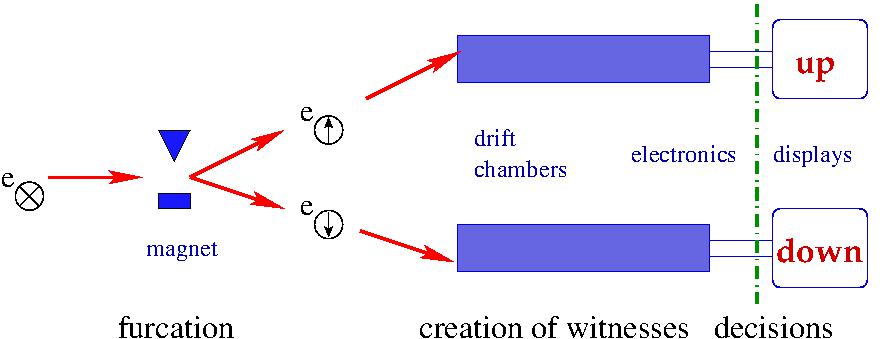
Figure 1: Stern-Gerlach measurement

We turn to an idealized Stern-Gerlach arrangement shown in figure 1. The wave function of an electron with a spin showing into the screen-plan gets separated in an inhomogeneous magnetic field into its up and down components both entering distinct drift chambers in which some electrons are knocked of their atoms and collected by a charged coupled electronics flushing “up” or “down” on display.

The process involves four essential parts:

furcation
witness production
alignment projection
choice decision

which will be explained below. They appear in all quantum measurements.

4 Furcation and witness production

At the furcation, the wave functions are split. The separation need not be geometrical; it must just enable the distinction in witness production in the next step. The furcation time can be much earlier than this next step. Furcated states (involving entangled partners) were shown to travel more than a thousand kilometers [27].

A vast number of low-energy photons typically dominate the witness production step. Most devices emit measurable Radio-frequency waves. Such photons with a wavelength between $0.03$ and $20$ meters carry unmeasurable energy of $10^{-23}$and $10^{-26}$ Joule, which means there are a lot of them. They are penetrating and have an excellent chance to escape the apparatus, the walls, and the ionosphere escaping into the open space.

For an expanding universe, it means they live practically forever. For simplicity, we will take the life-time of the universe, $t_{f}$, as finite. Presumably, in an eventually no longer interacting thin universe, the limit, $t_{f}\to\text{$\infty$}$, would exist.

In the setup of figure 1, the choice of the emitting drift chamber is in this way encoded in the hugely extended final state. It remains traceable. One can evolve the final state backward. As the photon number is large, one can disregard all components which interact before the drift chambers are reached. The procedure is not disturbed by the massive number of other witnesses.

In the quantum-dynamical evolution, many splittings and mergings contribute. We assume that this encoding of a splitting choice in the final state is a defining property of what has to be considered a quantum measurement.

To conclude, both processes, i.e., the furcation and the witness production, are still in the domain of quantum dynamics. However, they are essential ingredients of the measurement process. The measurement´s actual decisive part then has two parts: the alignment projection and the seemingly-random-choice decision.

5 Alignment decision

In QM, all combinations of components of the wave function and their conjugate coexist. The first reduction in the measurement decision is the alignment projection which selects matching components and eliminates mixed terms. Consider the up and down ones of the above’s setup. The alignment decision here introduces the following projection operator:

$$\;\begin{array}[]{ccc}P_{\mathrm{no\,interference}}(t)&=&|\uparrow>^{\mathrm{wave}}<\uparrow|\mathrm{{}^{wave}}\hskip 8.5359pt\otimes\hskip 8.5359pt|\uparrow>^{\mathrm{conjugate}}<\uparrow|\mathrm{{}^{conjugate}}\\ &+&|\downarrow>^{\mathrm{wave}}<\downarrow|\mathrm{{}^{wave}}\hskip 8.5359pt\otimes\hskip 8.5359pt|\downarrow>^{\mathrm{conjugate}}<\downarrow|\mathrm{{}^{conjugate}}\end{array}$$ (5)

This projection operator connects the wave function world and its conjugate. To illustrate how this happens, one can write equation 4 so that the part before the unit operator goes upward and the part after it goes downward, as done in equation 6. In this way, the vertically upward direction corresponds to the physical time direction denoted by $t$. The horizontal direction corresponds to the quantum operations order denoted as “quantum time,” by $\tau$.

  (6)

The projection operator which eliminates interference terms connects both sides. Both sides are otherwise not linked, and this simple addition seems to violate the spirit of a quantum dynamic-based theory.

In Bohmian mechanics [4, 11], the alignment follows from the assumption that the guided point particle does not live in wave function/conjugate quantum world and has to have one of the two values. Such an intrinsic automatic alignment also seems to apply to hidden variable theories [3, 22].

In objective-collapse theories [14, 10] the situation is more complicated. A new physical jump process introduces a projection operator:

$$P_{\mathrm{jump}}(t)=|\uparrow><\uparrow|\,\,\,\,\,+\,\,\,\,\,|\downarrow><\uparrow^{\prime}|$$ (7)

in the world or its complex conjugate. In equation 7, the meaning of $<\uparrow^{\prime}|$ is not clear. If one would assume $<\uparrow^{\prime}|\uparrow>\neq 0$, a first-order process in jump dynamic would exist, but $<i\,|\downarrow>^{\mathrm{world}}P_{\mathrm{jump}}<\uparrow|\,i>^{\mathrm{conjugate}}$ would introduce an angular dependence not seen in experiments. A second-order interaction is required acting on the wave function and its conjugate at the same time. The violation of the above separation postulate is therefore not avoided. Also, such new processes do require a relevant scale. As interference effects are observed at an astronomical scale [16], it is hard to explain how an objective-collapse theory could be used to understand table-top experiments.

Most seriously, in these theories or in a theory that adds the operator given in equation 5, it is not understood why witnesses´ production part is an essential ingredient of the measurement process. Therefore, we feel compelled to reject them.

It is widely agreed that decoherence [19] offers a simple mechanism to achieve the needed projection by eliminating interference contributions. The idea relies on that everything including witnesses from both sides have to agree. Traditionally witnesses are considered to reach an outside “macroscopic” domain where both components can no longer coexist separately and therefore have to coincide. However, there is not enough justification for adding such an extra outside domain as it can easily be avoided.

Let us look at the many world interpretation (MWI) [23] in a realist´s way. Each measurement decision results in a choice of separate worlds. It is not the furcation part but the witness production process which starts “new worlds.” A defining property of a separate world is that it can no longer merge with other worlds as different witnesses prevent such interference from different worlds for all future times, at least “for all practical purposes.” The outside macroscopic domain is not needed. It is replaced by some kind of boundary condition involving the witnesses.

Let us consider the way this alignment mechanism arises in a finite universe. Not requiring specific final properties replaces the final density matrix by the identity operator as it was done in equation 4. The identity operator then also involves the witnesses and requires them to match as pictured in equation 8:

                                                                            (8)

which effectively creates the required projection. The concept is attractive as no departure of quantum dynamics was required.

As a side remark, the concept contains some indirect backward causation on a wave function level. Decisions on the wave-function side determine the final state at $t_{f}$. The matching at $t_{f}$ introduced a projection affecting the complex conjugate wave function at much earlier times. However, backward causation on a quantum level does not exclude effective causality on a macroscopic level [6].

6 Seemingly-random-choice decision

The remaining projection implements the seemingly random choice between the different possible states. It is a central problem of quantum measurements, and many concepts were proposed. The most common implementation is just a randomly chosen projection operator in the wave function evolution or its conjugate

$$P_{\mathrm{jump}}(t)=|\uparrow><\uparrow|\,.$$ (9)

with a probability reflecting the size of the amplitude-squares. The introduction of the projection operator in the evolution

$$\begin{array}[]{c}<i\,|\,U(t-t_{i})\,P_{\mathrm{jump}}(t)\,U(t_{f}-t)\,|\,\boldsymbol{1}\,|\,U(t_{i}-t_{f})\,|\,i>\end{array}$$ (10)

can be written in a symmetric way relying on the alignment mechanism of the witnesses

$$\begin{array}[]{c}<i\,|\,U(t-t_{i})\,P_{\mathrm{jump}}(t)\,U(t_{f}-t)\,|\,\boldsymbol{1}\,|\,U(t-t_{f})\,P_{\mathrm{jump}}(t)\,U(t_{i}-t)\,|\,i>\,.\end{array}$$ (11)

In this expression, the projections mainly affect the future $t^{\prime}>t$ . However, the projection can also eliminate paths in the past. It is experimentally known that for entangled states, such backward correlations appear on a wave function level.

The Copenhagen interpretation tries to avoid backward causation by denying wave functions and fields ontological reality, which opens the door for intricate philosophical complications [13]. It seems largely successful except for quantum statistical effects, which introduce backward causation on a particle and not just on a wave-function level [5, 6, 7, 9]. The denial might have too much respect for classical physics and its concepts. Quantum mechanics with fields and wave functions is a beautiful well-tested theory with contains backward causation. The only requirement is that classical physics, with its seemingly causal behavior, emerges approximately to the degree and where we know it [6].

An intricate point concerns the probability with which the chosen contribution appears. The statistical relative weight of the decision at the time $t$ depends on on the wave function and its conjugate:

$$\frac{\begin{array}[]{c}<i\,|\,U(t-t_{i})\,P_{\mathrm{jump}}^{\uparrow}(t)\,U(t_{f}-t)\,|\,\boldsymbol{1}\,|\,U(t-t_{f})\,P_{\mathrm{jump}}^{\uparrow*}(t)\,U(t_{i}-t)\,|\,i>\end{array}}{\begin{array}[]{c}<i\,|\,U(t-t_{i})\,P_{\mathrm{jump}}^{\downarrow}(t)\,U(t_{f}-t)\,|\,\boldsymbol{1}\,|\,U(t-t_{f})\,P_{\mathrm{jump}}^{\downarrow*}(t)\,U(t_{i}-t)\,|\,i>\end{array}}\,.$$ (12)

It means that both sides are needed. Our quantum-dynamics-based postulate does not allow such a dependence except for the endpoints.

As said, in our epoch in the universe, typical witnesses live practically forever. Hence, the time - when the projection operator acts - is irrelevant. An obvious way to adhere to our postulate is to choose $t=t_{f}$ and we write for the probability of a particular jump choice:

$$\mathrm{prob(jump)}=\frac{<i\,|\,U(t_{f}-t_{i})\,P_{\mathrm{jump}}(t_{f})\,|\,\boldsymbol{1}\,|\,P_{\mathrm{jump}}^{*}(t_{f})\,U(t_{i}-t_{f})\,|\,i>}{<i\,|\,U(t_{f}-t_{i})\,|\,\boldsymbol{1}\,|\,U(t_{i}-t_{f})\,|\,i>}$$ (13)

The availability of surviving witnesses at $t=t_{f}$ determining the choice $P_{\mathrm{jump}}(t_{f})$ is, as said, taken as the definition of a true measurement process. There are many such branching processes in the evolution of the universe. They are defining a path, $Path_{k}$, in a huge tree in a many-worlds like structure. As there is no overlap between witness configurations, the path has to be equal on both sides, and one can write:

$$\sum_{\mathrm{all}\,k^{\prime}}<i\,|\,U(t_{f}-t_{i})\,Path_{\mathrm{k^{\prime}}}(t_{f})\,|\,\boldsymbol{1}\,|\,Path_{\mathrm{k^{\prime}}}^{*}(t_{f})\,U(t_{i}-t_{f})\,|\,i>=\boldsymbol{1}$$ (14)

where $Path_{\mathrm{k^{\prime}}}(t_{f})=P_{\mathrm{jump(1)}}^{k^{\prime}}(t_{f})\,\,\cdots\,\,\cdot P_{\mathrm{jump(n_{i})}}^{k^{\prime}}(t_{f})\,$ and the conjugation just changes the ordering.

The random choice decision has to select a given $path_{k}$ with a probability of the weight of the path

$$\mathrm{prob}(k)=<i\,|\,U(t_{f}-t_{i})\,Path_{\mathrm{k}}(t_{f})\,|\,\boldsymbol{1}\,|\,Path_{\mathrm{k}}^{*}(t_{f})\,U(t_{i}-t_{f})\,|\,i>$$ (15)

A computer program would first divide the state on both sides to mutually orthogonal path contribution, calculate their weight $\mathrm{prob}(k)$, and then choose a random number $RAND\in[0.1]$ and take the largest $k$ with $\sum_{k^{\prime}=1}^{k}\mathrm{prob}(k^{\prime})<RAND$ to select the chosen $path_{k}$. It is not a trivial task. The process should not affect self-organizing processes, which play an essential role in the evolution of the universe.

The obtained description is usually called two boundary quantum mechanics [17, 25, 26]. It is close to a multi-world interpretation in which the path is determined by a community of observers seeing identical measurement results. The probability of such a community witnessing the $path_{k}$ is determined analogously using equation 15. The matrix:

$$M_{\mathrm{all\,jumps}}(t_{f})=Path_{\mathrm{k}}(t_{f})\,|\,\boldsymbol{1}\,|\,Path_{\mathrm{k}}(t_{f})$$ (16)

is a hermitian with extremely tiny uncorrelated eigenvalues. This situation might allow approximating the matrix by the dominant vector product:

$$M_{\mathrm{all\,jumps}}(t_{f})=|t_{f}^{\mathrm{dominant}}><t_{f}^{\mathrm{dominant}}|\,.$$ (17)

In this way, one would obtain the two-state-vector interpretation of Aharonov and collaborators [1, 2].

The two-boundary and the two-state-vector descriptions are valid super-deterministic interpretations of QM [18]. However, the needed procedure to obtain equation 15 without affecting self-organization processes might be too complicated to accept. Also, such interpretations are incompatible with free will concepts.

There is a simple, natural way to select a path according to equation 15 [7], avoiding random selection. If desired, it can be easily amended to include free will decisions [8].

Consider the evolution of a state with a particular spin choice, say spin up, i.e., $<\uparrow(t)_{i}\,|$, in a universe originating in the initial state $<i\,|$ . If all final state $|f_{k}>$ are accepted unitarity leads to:

$$\sum_{\mathrm{all\,}k}<\uparrow(t)_{i}\,|\,U(t_{f}-t)\,|\,f_{k}>=1\,.$$ (18)

The probability of the up spin state choice reflects the production not considered in equation 18.

If the initial state on the wave function side $|\,i>$ differs from that on the conjugate side $|\,i^{\prime}>$ equation 4 changes to:

$$<i\,|\,U(t_{f}-t_{i})\,\boldsymbol{\boldsymbol{1}}\,U(t_{i}-t_{f})\,|\,i^{\prime}>\,\,\,\,\,\,\,\ll\mathrm{1}\,\,\,.$$ (19)

Considering the final universe´s rich structure, only a small region in the vast total Hilbert space involves each side´s final state. If the state $|\,i^{\prime}>$ is unrelated to $|\,i>$, the overlap (equation 19) can be expected to be tiny by many orders of magnitudes. For equation 18, it means:

$$\sum_{k\in\mathrm{overlapp}}<\uparrow(t)_{i}\,|\,U(t_{f}-t)\,|\,f_{k}>\,\,\,\,\,\ll\mathrm{tiny}\,\,\,.$$ (20)

The same holds for the down state.

In the considered experiment, we started at the time $t$ with a prepared in-the-screen-spin state $<\varotimes{}_{i}\,|\,$. The probability of measuring an up-spin state involves the absolute square of the amplitude:

$$\left|<\varotimes{}_{i}\,|\uparrow(t)_{i}>\sum_{k\in\mathrm{overlapp}}<\uparrow(t)_{i}|\,U(t_{f}-t)\,|\,f_{k}>\right|^{2}.$$ (21)

Statistically, two unrelated, extremely tiny quantities can not have a comparable magnitude, and one choice will dominate:

$$\begin{array}[]{ccc}\left|<\varotimes{}_{i}\,|\uparrow_{i}>\begin{array}[]{c}\sum\\ k\in\\ \mathrm{overlapp}\end{array}<\uparrow_{i}|U|f_{k}>\right|^{2}&\begin{array}[]{c}\gg\\ \mathrm{or}\\ \ll\end{array}&\left|<\varotimes{}_{i}\,|\downarrow{}_{i}>\begin{array}[]{c}\sum\\ k\in\\ \mathrm{overlapp}\end{array}<\downarrow_{i}|U|f_{k}>\right|^{2}.\end{array}$$ (22)

It will look like a random decision.

Averaging over many observations in different situations, one obtains:

$$\left[\left|\sum_{k\in\mathrm{overlapp}}<\uparrow_{i}|U|f_{k}>\right|^{2}\right]=\left[\left|\sum_{k\in\mathrm{overlapp}}<\downarrow_{i}|U|f_{k}>\right|^{2}\right]\,.$$ (23)

Moreover, the transition at a time t is independent of the environment. Hence, the Born term:

$$\left|<\mathrm{\varotimes}|\uparrow>/<\mathrm{\varotimes}|\downarrow>\right|^{2}$$ (24)

determines the relative contribution.

The obtained quantum decision is in some way like in a hidden variable theory. The “hidden” variable $\left(|\,i>-|\,i^{\prime}>\right)$ is, however, not affixed to individual observed particles but involves the whole universe. It determines the overlapping final density matrix, which then fixes the path of the measurement choices.

The presented concept also allows for this last step to stay in quantum dynamics. It is, therefore, without internal inconsistencies usually associated with measurements. Random decisions are gone, which is of fundamental importance. They were the reason why Einstein could not accept QM [12] as complete.

7 The surjection view of the evolution

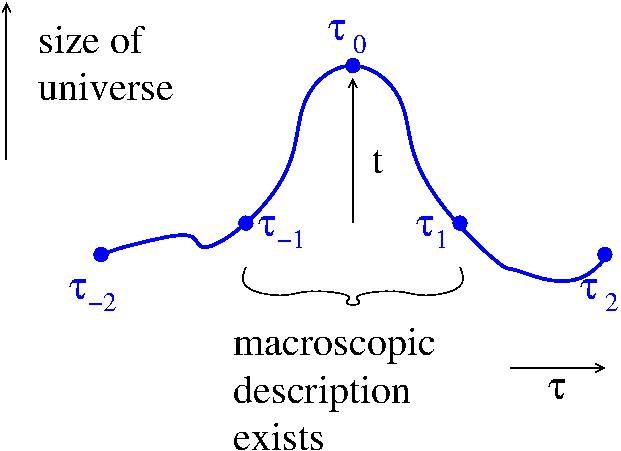
Figure 2: The surjection concept

Our interpretation is based on a surjection concept which changes our view of cosmological evolution. It considers a quantum universe starting, say, at a quantum time $\tau_{-2}$ reaching a huge maximal extension at a quantum time $\tau_{0}$ and ending at a quantum time $\tau_{2}$, as illustrated in figure 2. The quantum times $\tau_{-1}$ and $\tau_{1}$ lie in the expanding and contracting phase with an equal distance to the zenith, i.e. $(\tau_{0}-\tau_{-1})=(\tau_{1}-\tau_{0})$. Usually, no macroscopic, classical description is possible. An exception is a region between the quantum-times $\tau_{-1}$ and $\tau_{1}$. It involves a surjective mapping from a wave function $\psi(\tau)$ with $\tau\in[\tau_{-1},\tau_{0}]$ and a wave function $\psi(2\tau_{0}-\tau)$ with $(2\tau_{0}-\tau)\in[\tau_{0},\tau_{1}]$ to macroscopic object $\psi(2\tau_{0}-\tau)\cdot\psi(\tau)\approx\psi^{*}(t)\cdot\psi(t)$ with the real-time $t$ a monotonic function of $\tau-\tau_{-1}$. In simple words, we live with our wave function in the expanding quantum world and with our conjugate one in the contracting one.

Close to the zenith, one has $\psi(\tau_{0}+\epsilon)=\psi^{*}(\tau_{0}-\epsilon)$ . The quantum-times $\tau_{-1}$ and $\tau_{1}$ are chosen in a way that in the in-between region, the extensive system of witnesses matching in the extremely extended region at $\tau_{0}$ keep $\psi(2\tau_{0}-\tau)$ and $\psi^{*}(\tau)$ sufficiently close to maintain the usual prediction. Eventually, the different “initial” states

$$<i\,|=<\psi(\tau_{-2})\,|\mathrm{\,\,and\,\,}|\,i^{\prime}>=|\psi(\tau_{2})>$$

will yield $\psi(2\tau_{0}-\tau)\neq\psi^{*}(\tau)$ leading to visible CPT violations [8].

The required overlap at $\tau_{0}$ biases the contributing states at $\tau_{1}$ and $\tau_{-1}$. A more homogenous state at $\tau_{1}$ will at $\tau_{-1}$ have a larger domain close by with sufficiently matching partners than one with unregular structures. The - in this way - favored homogeneity in the early universe is observed. It is usually attributed to inflation [15].

8 Conclusion

Most of the spectacular successes of QM lie in the domain of quantum dynamics. We investigate how to add measurements and define four components. We observe that both setup components actually lie in the domain of quantum dynamics. The third component is the elimination of interference terms of components corresponding to different measurement results. The decoherence argument explains this contribution. If the argument is based on witnesses reaching the final state, it also manages to stay within the quantum dynamics domain.

We argue for a simple way to also reduce the seemingly random jump projections to the pure deterministic quantum dynamics. The universe´s lifetime is assumed to be finite with an open matching state at the final real-time. Two boundary states remain, the initial state on the wave function side and that on the usually just conjugate side. They are here taken as unrelated. Their difference acts as a hidden variable fixing a narrow matching state at the final time which then determines the seemingly random quantum choices. In this way, quantum measurements are embedded in entirely consistent quantum dynamics.

References

- [1] Yakir Aharonov, Peter G. Bergmann, and Joel L. Lebowitz. Time symmetry in the quantum process of measurement. Physical Review, 134(6B):B1410, 1964.
- [2] Yakir Aharonov, Eliahu Cohen, and Tomer Landsberger. The two-time interpretation and macroscopic time-reversibility. Entropy, 19(3), 2017.
- [3] John S. Bell. On the Einstein-Podolsky-Rosen paradox. Physics, 1(3):195–200, 1964.
- [4] David Bohm. A suggested interpretation of the quantum theory in terms of" hidden" variables. i. Physical review, 85(2):166, 1952.
- [5] Fritz W. Bopp. Strings and Hanbury-Brown-Twiss correlations in hadron physics. Theoretisch-Physikalischen Kolloquium der Universität Ulm, 15.November 2001.
- [6] Fritz W. Bopp. Time symmetric quantum mechanics and causal classical physics. Foundation of Physics, 47(4):490–504, 2017.
- [7] Fritz W. Bopp. A bi-directional big bang/crunch universe within a two-state-vector quantum mechanics? Foundations of Physics, 49(1):53–62, 2019.
- [8] Fritz W Bopp. How to avoid absolute determinismin two boundary quantum dynamics. Quantum Reports, 2(3):442–449, 2020.
- [9] Fritz W. Bopp. An intricate quantum statistical effect and the foundation of quantum mechanics. Foundations of Physics, 51(1):15, 2021.
- [10] Mark Davidson. Multi-valued vortex solutions to the Schrödinger equation and radiation. Annals Phys., 418:168196, 2020.
- [11] Detlef Dürr and Stefan Teufel. Bohmian mechanics. Springer, 2009.
- [12] Albert Einstein, Boris Podolsky, and Nathan Rosen. Can quantum-mechanical description of physical reality be considered complete? Physical review, 47(10):777, 1935.
- [13] Cord Friebe. Messproblem, Minimal- und Kollapsinterpretationen. In Philosophie der Quantenphysik, pages 43–78. Springer, 2015.
- [14] Gian Carlo Ghirardi, Alberto Rimini, and Tullio Weber. Unified dynamics for microscopic and macroscopic systems. Physical Review D, 34(2):470, 1986.
- [15] Alan H Guth. Inflationary universe: A possible solution to the horizon and flatness problems. Physical Review D, 23(2):347, 1981.
- [16] Robert Hanbury Brown and Richard Q. Twiss. Interferometry of the intensity fluctuations in light. I. Basic theory: the correlation between photons in coherent beams of radiation. In Proceedings of the Royal Society of London A: Mathematical, Physical and Engineering Sciences, pages 300–324. The Royal Society, 1957.
- [17] James B. Hartle. Arrows of time and initial and final conditions in the quantum mechanics of closed systems like the universe. arXiv:2002.07093, 2 2020.
- [18] Sabine Hossenfelder and Tim Palmer. Rethinking superdeterminism. Frontiers in Physics, 8:139, 2020.
- [19] Erich Joos, H. Dieter Zeh, Claus Kiefer, Domenico J.W. Giulini, Joachim Kupsch, and Ion-Olimpiu Stamatescu. Decoherence and the appearance of a classical world in quantum theory. Springer Science & Business Media, 2013.
- [20] Andrea Oldofredi and Cristian Lopez. On the classification between -ontic and -epistemic ontological models? Foundations of Physics, 50:1315–1345, 2020.
- [21] Jun John Sakurai and Jim J. Napolitano. Modern quantum mechanics. Pearson Higher Ed, 2014.
- [22] Gerard ’t Hooft. The Cellular Automaton Interpretation of Quantum Mechanics. Springer, 2016.
- [23] Lev Vaidman. Many-worlds interpretation of quantum mechanics. The Stanford Encyclopedia of Philosophy (Fall 2018 Edition), Edward N. Zalta (ed.), 2014.
- [24] John von Neumann. Method in the physical sciences, collected works, vol. 6; originally in l. leary (ed.): The unity of knowledge, 1955.
- [25] Ken Wharton. Time-symmetric boundary conditions and quantum foundations. Symmetry, 2(1):272–283, 2010.
- [26] Ken Wharton. Quantum Theory without Quantization. arXiv preprint arXiv: 1106.1254, 2011.
- [27] Juan Yin, Yu-Huai Li, Sheng-Kai Liao, Meng Yang, Yuan Cao, Liang Zhang, Ji-Gang Ren, Wen-Qi Cai, Wei-Yue Liu, Shuang-Lin Li, et al. Entanglement-based secure quantum cryptography over 1,120 kilometres. Nature, 582(7813):501–505, 2020.