Multiplicative noise underlies Taylor’s law in protein concentration fluctuations in single cells

Abstract

Protein concentration in a living cell fluctuates over time due to noise in growth and division processes. From extensive single-cell experiments by using E. coli strains with different promoter strength (over two orders of magnitude) and under different nutrient conditions, we found that the variance of protein concentration fluctuations follows a robust square power-law dependence on its mean, which belongs to a general phenomenon called Taylor’s law. To understand the mechanistic origin of this observation, we use a minimal mechanistic model to describe the stochastic growth and division processes in a single cell with a feedback mechanism for regulating cell division. The model reproduces the observed Taylor’s law. The predicted protein concentration distributions agree quantitatively with those measured in experiments for different nutrient conditions and a wide range of promoter strength. By using a mean-field approximation, we derived a single Langevin equation for protein concentration with multiplicative noise, which can be solved exactly to prove the square Taylor’s law and to obtain an analytical solution for the protein concentration distribution function that agrees with experiments. Analysis of experiments by using our model showed that noise in production rates dominates over noise from cell division in contributing to protein concentration fluctuations. In general, a multiplicative noise in the underlying stochastic dynamics may be responsible for Taylor’s law in other systems.

I Introduction

Protein concentrations inside a single cell determine functions and behaviors of the cell [1, 2, 3, 4, 5]. Given the small size of a cell, dynamics of protein concentration is highly stochastic and there is a significant cell-to-cell variability [6, 7, 8, 9, 10]. Protein concentration dynamics in a cell is determined by gene expression and protein synthesis processes as well as the growth and division processes of the cell, all of which can introduce significant noise [11]. These different sources of noise make it challenging to study statistics and dynamics of single cell protein concentration. Recently, advances in single-cell experimental techniques have started to shed lights on this difficult problem [12, 8, 13, 14]. One of the most revealing single cell measurements is done by using the so called “mother machine” where bacterial cells are constrained to grow and divide inside a microfluidic device [12, 15, 16], which allows simultaneous monitoring of the protein copy number as well as the cell length for many cell generations in a controllable and stable environment.

In this work, we studied the distribution of protein concentration in growing and dividing E. coli cells by using the mother machine microfluidic device. By measuring the single-cell protein concentration dynamics in a set of E. coli strains with different promoter strength, we found that the variance of the single cell protein concentration fluctuations is proportional to the square of the mean for all strains over a wide range (over $10^{2}$ fold change) of the mean protein concentration. Furthermore, we found that the scaled protein concentration distribution follows a universal function independent of the specific value of the mean. A power law scaling relationship between variance and mean is generally called the Taylor’s law, which is named after Lionel Taylor who first observed it in ecology [17] and later found to exist in diverse fields from number theory to epidemiology [18, 19, 20, 21].

The protein copy number fluctuations were studied in E. coli by Salman et al [22], where a square dependence of the mean of the protein number with respect to the variance was first reported. By using a phenomenological model [4, 23], Brenner et al showed that the protein number $N$ in a growing and dividing cell follows approximately a log-normal distribution with a constant variance under the assumption that $N$ increases exponentially with respect to time. The only protein number scale comes from the mean, which is fixed in the phenomenological model as a mathematical constraint. This result is a particular case of a previous more general work on population growth in a stochastic environment by Lewontin and D. Cohen [24], which was later linked to the Taylor’s law by J. Cohen et al. [25, 26].

However, while previous models [4, 23] were able to explain the Taylor’s law in protein number fluctuations phenomenologically, it can not be used to explain fluctuations of protein concentration, which depend on fluctuations in both protein number and cell size. Since gene expression and cell size have correlated yet different dynamics during growth and division, the challenge for explaining the observed Taylor’s law in protein concentration fluctuations can only be met by understanding both the protein number and cell size dynamics consistently in a growing and dividing cell.

In a single cell, dynamics of the protein number (for a particular protein) and the cell size are correlated since they are controlled by the same ribosome-based protein production machinery as well as the same cell division events. However, their dynamics are not identical. For the growth process, since cell size growth involves production of a combination of different proteins/biomolecules, the instantaneous cell size growth rate will be different from that for a particular protein. When a cell divides, the partition factor (the fraction that goes into the daughter cell) is different for a particular protein than for the cell size. These differences are easy to appreciate as there would be no protein concentration fluctuations if their dynamics were identical.

To understand the origin of the observed Taylor’s law in protein concentration fluctuations, we developed a simple unified model to describe dynamics of both protein number and cell size during growth and division. In the model, the growth of both protein number and cell size depend on the number of a common production machinery (complex) with production (growth) rates different for protein number and cell size. The production machinery, which can be characterized by the number of ribosomes ($R$) in the cell, has its own dynamics, which is controlled by the same production and division processes as for a specific protein. Instead of enforcing a mean protein number as an ad hoc mathematical constraint as in previous models for protein number fluctuations [23] and cell size regulation [27], a division control variable (molecule $Z$) is introduced in our model. $Z$ also follows the same production and division dynamics as that of a protein (or $R$). The probability of cell division increases sharply when the number of molecule $Z$ crosses a certain threshold $Z_{0}$ [28, 29, 30, 31, 32]. In this paper, we use this minimal mechanistic model to study protein concentration fluctuations and compare the theoretical results quantitatively with single cell data from the mother machine experiments.

II Results

A Protein concentration fluctuations follow Taylor’s law

We constructed a set of E. coli strains that produce the fluorescent protein Venus (Fig. 1A). Each strain contains a plasmid that expresses the Venus gene controlled by a promoter from a set of constitutive promoters with different strengths (see Appendix A for details about the experiments) [33]. Using the mother machine technique [15, 12, 8, 10], and fluorescent microscopy, we monitored individual cells of such strains under steady-state conditions, with a constant flow of either rich or poor media. For each combination of nutrient conditions and promoter strength, we measured the cell size and the fluorescent intensity protein for $\sim 20$ different mother cells and $\sim 50$ cell generations per mother cell. We assume that the intensity of the fluorescence of a cell at time $t$, $N(t)$, is proportional to the number of Venus protein, and thus the fluorescence density (fluorescence divided by cell size, indicated as $c$) can be considered a proxy of the protein concentration.

In Fig. 1B we show a typical time trace of the normalized cell length (size) $L$ (top), total fluorescence $N$ (middle), and fluorescence density $c(\equiv N/L)$ (bottom) for many cell generations. Both protein number (fluorescence intensity) and cell length follow continuous exponential growth that is interrupted by periodic “discontinuous” reductions due to cell division. The fluorescence density $c$ is much more continuous than $N$ and $L$ and the influence of cell division is not strong. This is easy to understand because the gross effect of cell division for both $N$ and $L$ is canceled out in $c$. However, even though cell division does not affect the protein concentration the same way as the protein number or cell size, we also note from Fig. 1B (bottom) that there is a small but observable change in $c$ at cell division times (red dots), which suggests that cell division is likely a source of noise for protein concentration.

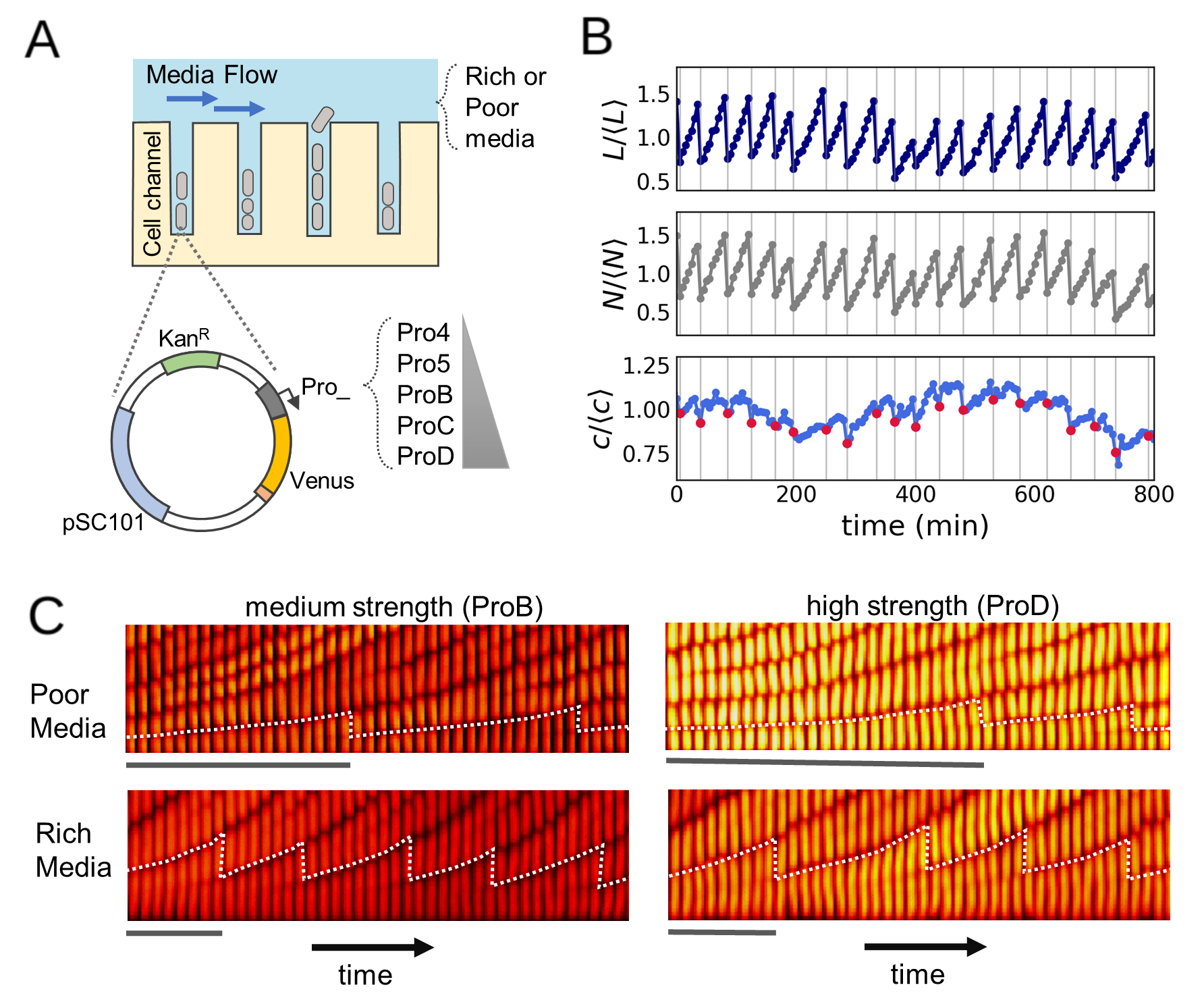
Figure 1: (A) Schematics of the experimental setup. Using the microfluidic device mother machine and fluorescent microscopy, we monitored individual cells of various E. coli strains growing under a constant flow of either rich or poor media. Each strain contains a plasmid that codifies for the fluorescent protein Venus under the control of an artificial promoter from a set of promoters with increasing strengths, Pro{4,5,B,C,D} [33]. (B) Typical time traces of a single cell containing the ProB promoter and growing in rich medium: normalized cell length $L$ (top), total fluorescence $N$ (middle), and fluorescence density $c$ (bottom). The vertical lines and the red dots in the bottom plot indicate the time of a cell division. (C) Kymographs illustrating the fluorescence level of strains with the promoters ProB (left) and ProD (right) controlling Venus expression, growing in poor (top) and rich (bottom) media. Each frame is separated from the following one by a time interval of 5 minutes. The bars below the kymographs show the span of a cell trace from birth until division.

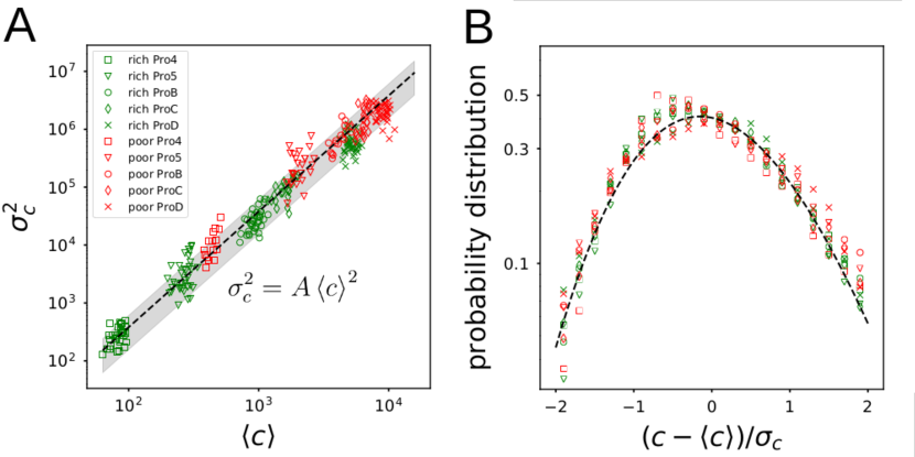
Figure 2: The Taylor’s law and the universal distribution of the normalized protein concentration fluctuations. (A) Variance ($\sigma_{c}^{2}$) of the protein concentration versus the mean value ($\langle c\rangle$) for individual cells. The poor and rich nutrient conditions are labeled by red and green colors, respectively. Different symbols correspond to cells with different promoters. All data from different cells with different promoters and growth condition follow the square Taylor’law: $\sigma_{c}^{2}=A\langle c\rangle^{2}$ with $A=0.038\pm 0.015$. The black dashed line and the gray thick line around it reflect the mean and standard deviation of $A$. (B) Distributions for the normalized fluctuations of $c$ for different nutrient conditions and promoter strengths shown in (A) collapse. The dashed line is obtained from the analytical expression Eq. 11 from our model.

To study how fluctuations in cell size and protein number depend on the mean growth and transcription rates, we did experiments using several constitutive promoters with different strengths [12] and also with two nutrient (growth) conditions [8]. Qualitatively, as shown in Fig. 1C, a stronger promoter leads to a higher fluorescence intensity; whereas a rich nutrient condition leads to a faster growth and a shorter average division time $\Delta T$.

From each combination of promoter and growth condition, we determined the distribution of the protein concentration, $P(c)$, from measurements such as those shown in Fig. 1 for many ($\sim 20$) individual mother cells. From the distribution, we computed the mean $\langle c\rangle$ and the variance $\sigma_{c}^{2}$. As shown in Fig. 2A, the variance and the mean follow the square Taylor’s law, i.e., the variance $\sigma_{c}^{2}$ is proportional to the square of the mean $\left<c\right>$:

$$\sigma_{c}^{2}=A\left<c\right>^{2}\,,$$ (1)

with the prefactor constant $A$ within a narrow range $A=0.038\pm 0.015$ for all promoters and nutrient conditions studied in this paper. This is remarkable considering that the power law scaling relation (Eq. 1) is valid for two orders of magnitude of $\left<c\right>$ across different promoter strength and nutrient conditions. Moreover, the probability distributions of the normalized concentration $(c-\left<c\right>)/\sigma_{c}$ for all promoters and nutrient conditions collapse onto the same universal curve as shown in Fig. 2B. In the following sections we develop a mechanistic model to explain these experimental results.

B A minimal model for growth and division explains Taylor’s law

Cell growth and division are complex processes involving many regulatory proteins and pathways, which are beyond the scope of this paper. Here, we aim to develop a simple model that captures the most salient features in the underlying molecular mechanism governing protein concentration fluctuations in growing and dividing cells in a mother machine setup. In the minimal model, the growth and division processes in a cell are controlled by a production variable $R$ and a division variable $Z$, respectively. All dynamic variables in a cell such as the cell length $L$, protein number $N$, as well as $R$ and $Z$ themselves are controlled by $R$ and $Z$.

A common production variable $R$ that is shared by other variables of the system is supported by the fact that growth rates of $L$ and $N$ during cell growth are not independent. As shown in Fig. 3A, during each growth period between two consecutive divisions, we can fit the cell length and protein number dynamics to exponential functions and determine the growth rates $\lambda_{l}$ and $\lambda_{n}$ for $L$ and $N$, respectively. In Fig. 3B, we plot $\lambda_{n}$ versus $\lambda_{l}$ for all growth periods and for all three nutrient conditions, which clearly shows that the two growth rates are highly correlated. To account for this strong correlation, all growth rates in our model are assumed to be proportional to the common production variable $R$, which can be interpreted as the number of active ribosomes in the cell. In previous experiments [34], it was shown that the growth rate depends linearly on the RNA/protein ratio. Since the total RNA content in a cell is a good measure of the ribosome number, these experiments support the assumption that growth rates are proportional to $R$.

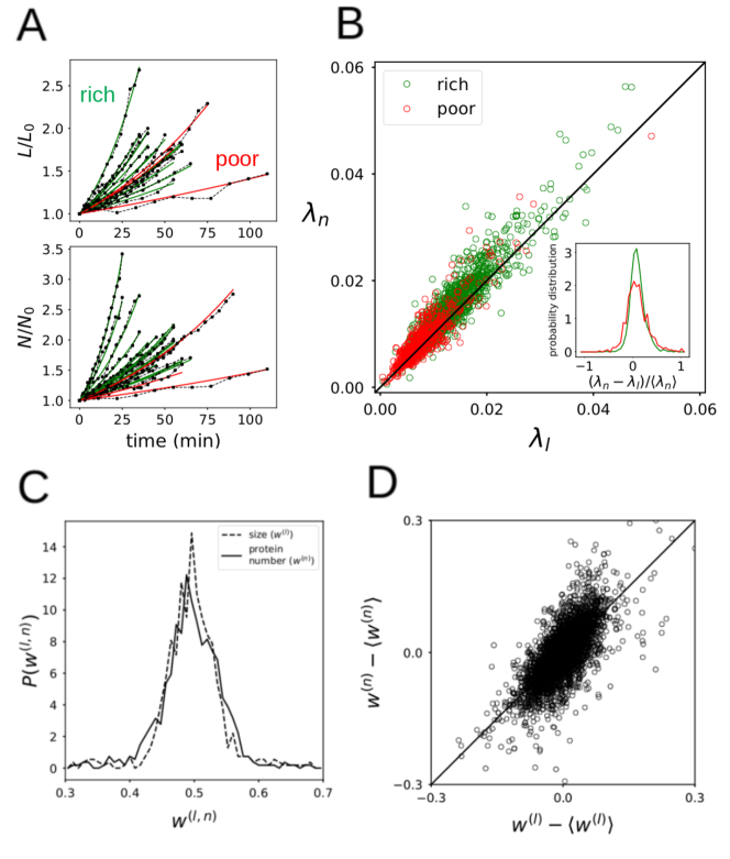
Figure 3: Noise sources due to growth and division. (A) The effective growth rates $\lambda_{l}$ and $\lambda_{n}$ were obtained by fitting the cell size and protein number dynamics during each growth period (between two consecutive division events) with exponential functions. An example of the fitting is shown for $L$ (top) and $N$ (bottom), different colors correspond to different nutrient conditions. (B) $\lambda_{l}$ versus $\lambda_{n}$ shows high but not perfect correlation. Deviations from the diagonal black line correspond to a noise source for $c$ due to growth. The inset shows the distribution of the relative difference between $\lambda_{l}$ and $\lambda_{n}$. (C) Distribution of the partition factors $w^{(l,n)}$ for cell size and protein number. (D) The correlation between $w^{(l)}$ and $w^{(n)}$ is high but not perfect. Deviations from the diagonal black line correspond to another noise source for $c$ due to division.

In order to maintain cell size homeostasis, a feedback mechanism is needed to control cell division. Indeed, as pointed out in  [23, 4], if cell divisions were to occur at independent random time intervals, even with a fixed mean the accumulation of variation in division times away from their mean would lead to divergence of cell length fluctuation. In bacterial cells, cell division is regulated by the division protein FtsZ [35, 36, 37], which assemble into a ring (the Z ring) localized at the future division site of the cell. The completion of the Z ring, together with other proteins, is critical for cell division. Motivated by these experimental facts and by following previous theoretical work [28, 29, 30, 31, 32], we assume that the probability for cell division increases sharply with $Z$ when $Z$ crosses certain threshold $Z_{0}$. Since the Z ring formation depends on oligomerization of FtsZ at a localized site the threshold is set over the total number of proteins as opposed to its concentration.

Taken together, our model is represented schematically in Fig. 4A (top). There are $4$ extensive variables: the cell size (length) $L$ and the protein number $N$ are “observable” variables that can be directly measured in the mother machine experiments; the number of growth complexes (ribosomes) $R$ and the number of division proteins (FtsZ) $Z$ are “hidden” variables that control the growth and division of all variables including themselves. The stochastic dynamics of the $4$ variables in the mother cell are described by the following stochastic ordinary differential equations:

$$\frac{dL}{dt} =R\,K_{l}(1+\eta_{l})-L\sum^{n_{d}(t)}_{i=1}w^{(l)}_{i}\,\delta(t-t_{i}(Z)),$$ (2)

$$\frac{dN}{dt} =R\,K_{n}(1+\eta_{n})-N\sum^{n_{d}(t)}_{i=1}w^{(n)}_{i}\,\delta(t-t_{i}(Z)),$$ (3)

$$\frac{dR}{dt} =R\,K_{r}(1+\eta_{r})-R\sum^{n_{d}(t)}_{i=1}w^{(r)}_{i}\,\delta(t-t_{i}(Z))$$ (4)

$$\frac{dZ}{dt} =R\,K_{z}(1+\eta_{z})-Z\sum^{n_{d}(t)}_{i=1}w^{(z)}_{i}\,\delta(t-t_{i}(Z)),$$ (5)

which all have the same general form. The first and second terms on the right side of each equation represent effects of growth and division, respectively. The parameters $w^{(j)}_{i}$ ($j=n,l,r,z$) are the partition factors, which is the fraction of variable (protein number) $j$ that goes to the tracked daughter cell upon the $i$-th division event; $t_{i}(Z)$ is the time of the $i$-th division that depends on $Z$ (see below); $K_{j}$ ($j=n,l,r,z$) are the mean growth (production) rates; $\eta_{j}$ ($j=n,l,r,z$) are the fractional noise in growth rates, which are taken to be Gaussian white noise here with zero mean and variance $\Delta_{j}$; and $n_{d}(t)$ is the number of divisions up to a time $t$: $n_{d}(t)=\int_{0}^{t}\,dt^{\prime}\sum^{\infty}_{i}\delta(t^{\prime}-t_{i}(Z))$.

The feedback control for cell division is modeled here by a soft-thresholding process with a simple logistic function (Fig. 4A (bottom)):

$$P_{d}(Z)=\frac{\Delta t^{-1}}{1+\exp\left[(Z_{0}-Z)/\Delta Z\right]}$$ (6)

which is characterized by three parameters each with clear biological meaning. The threshold value $Z_{0}$ is the value of $Z$ at which the division probability increases sharply, with the sharpness determined by $\Delta Z\ll Z_{0}$ ($P_{d}$ is simply a step function when $\Delta Z=0$). Once cell division starts, it can take a finite time to complete. This small but finite time scale is given by $\Delta t$ in Eq. 6. Other forms of $P_{d}(Z)$ with the same general properties considered here were used without affecting the general results. The choice of parameters used in our simulations is discussed in Appendix B.

There are two sources of noise due to fluctuations in growth rates and in partition factors, respectively. The noise in growth rates ($\eta_{n,l}$) for $N$ and $L$ can be estimated from measurements and analysis shown in Fig. 3A&B. Similarly, the noise in partition factors ($w^{(n,l)}$) can be determined from the measured distributions for $w^{(n,l)}$ as shown in Fig. 3C. Though there is a strong correlation between these two partition factors (Fig. 3D), their difference remains significant and it gives rise to another source of noise for $c$.

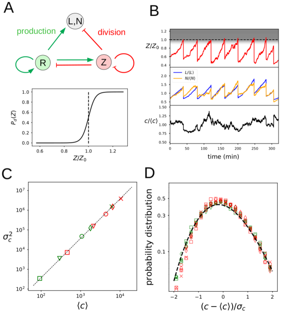
Figure 4: The minimal mechanistic model and its behaviors. (A) Top: Illustration of the 4-node model. All production (growth) processes (green arrows) depend on $R$. The division process, which reduces all variables (red lines), is controlled by $Z$. Bottom: the probability rate of division $P_{d}(Z)$ as a function of the division protein number $Z$. (B) Time traces of normalized division protein (red), protein number $N$ (orange), cell size $L$ (blue), and protein concentration $c=N/L$ (black). In the top panel we show in gray the region where the division probability is large (the dotted line is for $Z=Z_{0}$). (C) Variance of the concentration versus its mean from our model for different promoters (different symbols) and under different nutrient conditions (green: rich medium; red: poor medium). The same symbols and colors are used as experimental data shown in Fig. 2A for easy comparison. (D) Distributions of the normalized fluctuations in the concentration obtained with the same parameters as in (C) collapse onto the same curve. The dashed line is from the analytical expression Eq. 11 obtained from our model. The parameters for $P_{d}(Z)$ were $\Delta Z/Z_{0}=2.7\times 10^{-2}$ and $\Delta t=2\,\mbox{min}$. See Appendix B for details of the simulations and parameters used.

We studied our model by solving the stochastic equations (Eqs. 2-5) numerically with physiologically reasonable parameters, some of which are estimated from the mother machine experiments. In Fig. 4B, we show the time traces of different variables as well as the dynamics of the protein concentration. The cell division control by the variable $Z$ can be seen from the top panel in Fig. 4B which shows that $Z$ follows the same growth and division dynamics as other variables and division occurs with a high probability as $Z$ (red) crosses over the threshold $Z_{0}$ (dashed line). As shown in the middle panel in Fig. 4B, both $L$ (blue) and $N$ (orange) follows the same general growth and division pattern as that of $Z$, but their dynamics are not identical. As a result, the protein concentration $c$ (black) shows smaller but finite and continuous fluctuations that are different from those in $N$ or $L$. The behaviors of $N$, $L$, and $c$ from our model resemble closely with those from experiments shown in Fig. 1.

We also studied cell size homeostasis during growth [8, 38], i.e., the dependence of elongation $\Delta L$ and division time $\Delta T$ on initial cell size $L_{0}$ during each cell cycle under different growth conditions. The model results are in quantitative agreement with experiments, which validates the model for describing cell growth and division (see Appendix C for details).

To quantitatively compare the results from the model with the experimental results, we tune the rates ($K_{n,l,r,z}$) and the noise strength ($\Delta_{n,l,r,z}$), in accordance with experimental data for different promoters and in different nutrient conditions. Given that the promoter strength primarily influences the expression rate of the corresponding proteins, we assumed that the change in promoter is captured in the model by a change in the value of $K_{n}$, so that the rate of increase in $N$ would be directly affected. The mechanism by which nutrient condition influences the kinetic rates of growth and expression is beyond the scope of this work. Here, we treat the nutrient dependence within our model phenomenologically based on experiments. In particular, from the experiments, the average division time $\left<\Delta T\right>$ is longer in the poor nutrient condition, whereas the average length size $\left<L\right>$ is smaller. We find that the simplest way to account for this observed difference in our model is by assuming that the production rate for the division variable $Z$, $K_{z}$, is roughly independent of nutrient conditions while the other two rates for growth-related variables ($R$ and $L$) are scaled by a common nutrient-dependent constant $\xi$, i.e., $K_{i}\rightarrow\xi K_{i}$ with $i=r,l$ with $\xi=1$ for rich medium and $\xi=0.6$ for poor medium (see Appendix C for details). Operationally, we first tune $K_{l}$ and $K_{r}$ to match the observed cell growth statistics in different nutrient condition before we tune $K_{n}$ to properly fit the value of $\left<c\right>$. See Appendix B for details of the simulations and parameter choice.

As shown in Fig. 4C, where the variance of $c$ is plotted as a function of its mean, the simulation results from our model obey the same square Taylor’s law as in the experiments with the coefficient of proportionality $A=0.034\pm 0.006$ that is in quantitative agreement with the experiments. Furthermore, the normalized distribution function for $c$ shows the same collapse for all values of $K_{n}$ as shown in Fig. 4D.

C Multiplicative noise underlies Taylor’s law in protein concentration fluctuations

In the previous section, we studied protein concentration fluctuations by simulating the full model (Eqs. 3-5) numerically. Here, we show the emergence of Taylor’s law by using a mean field approximation, which leads to a closed form relation between the variance and the mean of $c$ and an analytical expression for the probability distribution of $c$. We start by considering the equation for $c$, obtained from Eqs. 2&3 (see Appendix D for details):

$$\frac{dc}{dt}=\hat{K}_{n}-\hat{K}_{l}\,c+c\sum_{i}^{n_{d}(t)}\left[\left(w_{i}^{(l)}-w_{i}^{(n)}\right)\delta(t-t_{i})\right]\,,$$ (7)

where we have defined the effective rates $\hat{K}_{l}=rK_{l}(1+\eta_{l})$ and $\hat{K}_{n}=rK_{n}(1+\eta_{n})$, with $r=R/L$. The difference $\delta w_{i}=w_{i}^{(l)}-w_{i}^{(n)}$ has zero mean $\left<\delta w_{i}\right>=0$ and a delta-function correlation $\left<\delta w_{i}\delta w_{j}\right>=2\Delta_{w}\delta_{ij}$ as $\delta w_{i}$ for different division events can be considered independent. For a time scale longer than the average division time $\langle\Delta T\rangle$, we can define an average (mean-field) cell division noise $\eta_{d}$ whose correlation has the form $\left<\eta_{d}(t_{1})\eta_{d}(t_{2})\right>=2\Delta_{d}\delta(t_{1}-t_{2})$ with $\Delta_{d}=\Delta_{w}/\left<\Delta T\right>$ the cell division noise strength. The variables $\hat{K}_{l}$ and $\hat{K}_{n}$ in Eq. 7 can be written as: $\hat{K}_{l,n}=\left<\hat{K}_{l,n}\right>(1+\chi_{l,n})$ where $\chi_{l,n}=\frac{\delta r}{\langle r\rangle}+\eta_{n,l}$ is the fractional noise with $\delta r(=r-\langle r\rangle)$ and $\langle r\rangle$ the fluctuation and the mean of $r$. Thus, by taking the mean-field approximation in the long time limit, the Langevin equation (Eq. 7) can be re-written as:

$$\frac{dc}{dt}=\left[\left<\hat{K}_{l}\right>(\mu-c)+\mu\eta_{a}+c\eta_{m}\right]\,,$$ (8)

where $\mu=\left<\hat{K}_{n}\right>/\left<\hat{K}_{l}\right>$ is the average of $c$: $\langle c\rangle=\mu$, which is varied experimentally by changing the promoter strength or the nutrient condition, whereas $\eta_{a}=\left<\hat{K}_{l}\right>\chi_{n}$ and $\eta_{m}=\eta_{d}-\left<\hat{K}_{l}\right>\chi_{l}$ are the two noise terms for $c$.

It is interesting to note that both noise terms ($\eta_{a}$ and $\eta_{m}$) in Eq. 8 are multiplied by either the mean concentration ($\mu$) or the instantaneous concentration ($c$) itself. As a result of the multiplicative nature of the noise terms, Eq. 8 is invariant if $c$ and $\mu$ are scaled by an arbitrary constant factor. This scale invariance immediately suggests that the distribution of $c/\mu$ is independent of $\mu$ and the variance is proportional to the square of the mean. Indeed, by solving the Fokker-Planck equation corresponding to Eq. 8, we derive an exact relationship between the variance and the mean (see Appendix E for details):

$$\sigma^{2}_{c}=A\left<c\right>^{2}\,,$$ (9)

and the prefactor $A$ can be determined analytically:

$$A=\frac{\Delta_{g}+\Delta_{d}}{\left<\hat{K}_{l}\right>-\Delta_{m}}\,,$$ (10)

where $\Delta_{g}=\left<\hat{K}_{l}\right>^{2}(\Delta_{n}+\Delta_{l})$ is the strength of the growth-dependent noise due to fluctuations in growth and production rates for cell size ($\Delta_{l}$) and protein number ($\Delta_{n}$); $\Delta_{m}=\Delta_{d}+\left<\hat{K}_{l}\right>^{2}(\Delta_{(r)}+\Delta_{l})$ is the strength of the noise $\eta_{m}$ with $\Delta_{(r)}$ the noise strength for $\delta r/\langle r\rangle$.

Eq. 9 is a direct confirmation of the Taylor’s law, with the same exponent $p=2$ as observed in experiments. Moreover, the analytical expression for the prefactor constant $A$ (Eq. 10) reveals explicitly that both the growth rate noise ($\Delta_{g}$) and the cell-division partition noise ($\Delta_{d}$) contribute to $A$. These noise strength ($\Delta_{g}$ and $\Delta_{d}$) can be determined quantitatively. For example, in our model (Eqs. 2-5) with a typical set of parameters that fit the averaged experimental results shown in Fig. 4, the noise strengths from division and growth can be obtained: $\Delta_{d}=3.7\times 10^{-5}\,\mbox{min}^{-1}$, $\Delta_{g}=3.5\times 10^{-4}\,\mbox{min}^{-1}$, which shows that the contribution from growth rate fluctuations is $\sim 10$-fold stronger than that from cell division. Analysis of different noise sources for experiments with different strains under different growth conditions confirms that the noise from growth rate fluctuation is in general stronger than that from the partition error during cell division (see Table 2 in Appendix F). Our analysis also shows that the average value of $A$, which is a measure of overall noise, is slightly smaller in rich medium than that in poor medium. However, the difference in the average $A$ between the two nutrient conditions is relatively small and is comparable with the difference in $A$ among individual cells with the same promoter and under the same nutrient condition (See Fig. 7 in Appendix F for a detailed comparison).

Finally, by solving the steady state Fokker-Planck equation for Eq. 8, we obtain an analytical expression for the distribution function of $c(\geq 0)$:

$$P(c)=\frac{1}{Z}\left(\frac{\mu^{2}\Delta_{a}+2\mu\Delta_{am}c+\Delta_{m}c^{2}}{\left<\hat{K}_{l}\right>}\right)^{-1-\frac{\left<\hat{K}_{l}\right>}{2\Delta_{m}}}\exp\left[\frac{2\left<\hat{K}_{l}\right>(\Delta_{am}+\Delta_{m})\tan^{-1}\left[\frac{\mu\Delta_{am}+\Delta_{m}c}{\mu\rho_{\Delta}}\right]}{2\Delta_{m}\rho_{\Delta}}\right]\,,$$ (11)

and $P(c<0)=0$ where $Z$ is the normalization constant, $\Delta_{a}=\left<\hat{K}_{l}\right>^{2}(\Delta_{(r)}+\Delta_{n})$ is the noise strength for $\eta_{a}$, $\Delta_{am}=-\left<\hat{K}_{l}\right>^{2}\Delta_{(r)}$ is the correlation between $\eta_{a}$ and $\eta_{m}$, and $\rho_{\Delta}=\sqrt{\Delta_{a}\Delta_{m}-\Delta_{am}^{2}}$. There is a negligibly small value for $P(c)$ at $c=0$, which is caused by assuming $\eta_{a}$ to be an unbounded Gaussian noise. For large $c\gg\mu$, $P(c)$ decays as a power law $\sim c^{-2(1+\frac{\left<\hat{K}_{l}\right>}{2\Delta_{m}})}$, which is different from a log-normal distribution but similar to an inverse Gamma distribution, which is the solution for $P(c)$ in the limit of negligible addition noise ($\Delta_{a}=\Delta_{am}=\rho_{\Delta}=0$). In Figs. 2B&4D, we plotted the analytical distribution function given in Eq. 11 (black dashed line), which quantitatively agrees with experimental results and simulation results from the full stochastic model.

III Discussion

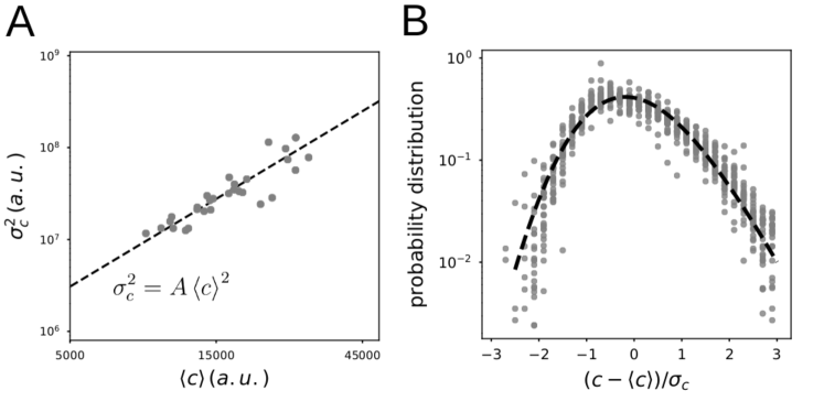
Figure 8: (A) Mean of the fluorescence density $c$ as a function of the variance from the experimental data obtained in [22]. The dashed line is obtained using an average value for the coefficient $A=\sigma_{c}^{2}/\left<c\right>^{2}$. The value obtained in this set of data was $\left<A\right>=0.12$. (B) The scaled protein concentration distributions from the experimental data reported in  [22]. The black curve is the distribution that we show in the main text.

In this paper, we developed a minimal mechanistic model to study stochastic dynamics of protein concentration in single cells over a long timescale that spans many generations. The balance between growth and division processes is key to maintain a dynamic equilibrium for cells. Here, we showed that the stochastic growth and division processes in a single cell are the two dominant noise sources contributing to fluctuations in protein concentration. By considering these two stochastic processes explicitly and consistently in our model, we were able to obtain the square variance-mean scaling relation (Taylor’s law) as well as the universal distribution for the normalized concentration, both of which are in quantitative agreement with our mother machine experiments with different promoters and under different nutrient conditions. We have used our model to analyze previous experiments [22] under different experimental conditions and obtained consistent results although the data there cover a much smaller range ($\sim 1/2$ decade) of mean protein concentrations (see Fig. 8 in Appendix for details).

There are two central regulatory variables in our model, $R$ and $Z$, which control growth and division, respectively. Both $R$ and $Z$ can be considered as large complexes with multiple components, however, each of them has identifiable key components: $R$ is associated with ribosome, whereas $Z$ is associated with FtsZ. In our minimal model, we only implemented the simplest possible interactions between $R$ and $Z$ – the growth rates of all proteins (including $R$ and $Z$ themselves) are proportional to $R$; and the probability of cell division increases sharply when $Z$ crosses a certain threshold $Z_{0}$. Despite its simplicity, the minimal model is able to reproduce the observed statistics of protein concentration fluctuations and cell size homeostasis. More importantly, the minimal model provides a mathematical framework to ask further questions regarding molecular origins of the growth and division processes. For the division control, one key question is about the molecular origin for the cell division regulation, which is modeled here by the assumption (hypothesis) that the probability of division increases sharply when $Z$ crosses a threshold $Z_{0}$. For the growth process, we did not take into account the way resources are allocated to the production of different protein classes in our model where all production rates are linearly proportional to $R$. The effect of proteome allocation can be studied in our model by allowing different substrates (mRNA’s) to compete for the same finite pool of $R$ with different affinities, which results in a nonlinear dependence of the production rates on $R$. It would be interesting to study proteome allocation [39] in dividing cells by introducing nonlinear growth rates in our model.

In this paper, we focused on explaining the square Taylor’s law (TL) with $p=2$ for protein concentration fluctuations. However, our model also indicates how the exponent $p$ may deviate from $2$. In particular, from the analytical expression for the variance-average dependence (Eq. 9), it is easy to see that if the prefactor $A$ is correlated with the mean $\mu(\equiv\langle c\rangle)$, then the variance-mean relation would deviate from the square TL, e.g., if $A$ depends on $\mu$ in a power law form, $A\sim\mu^{\alpha}$, then the variance-mean relation follows the TL with an exponent $p=2+\alpha$. From the expression for the prefactor $A$ (Eq. 10), such a correlation can be introduced by having a correlation between the noise strength ($\Delta_{g,d}$) and $\mu$ and/or a correlation between the time scale $\tau_{c}\equiv\langle\hat{K}_{l}\rangle^{-1}$ and $\mu$. In our experiments, the mean concentration is varied by changing the promoter strength characterized by $K_{n}$ in our model. Since $K_{n}$ does not appear in the expression for $A$, there is no correlation between $A$ and the mean $\mu$, which leads to the observed square TL. However, $\mu$ also depends on the elongation rate $K_{l}$, which affects $A$. Therefore, if the mean concentration $\mu$ can be varied by changing the elongation rate $K_{l}$, our model would predict a deviation from the square TL, which may be tested experimentally.

Taylor’s law is an ubiquitous scaling law observed in a plethora of different systems, from the occurrence of measles cases [20] to the share price fluctuations in stock market [40]. However, these observations of Taylor’s law remain largely empirical with little understanding of their mechanistic origins. Here, we showed that the square Taylor’s law (exponent $p=2$) exists generally in systems whose stochastic dynamics can be described by a Langevin equation with multiplicative noise, i.e., the noise term is multiplied by the variable of interest. Even though we focused on studying protein concentration fluctuations in bacterial cells such as E. coli, the general theoretical framework used in this paper may be applicable to other systems where the dominant noise source is multiplicative. Different TL exponents observed in different systems may be caused by possible correlations between key parameters in the system (e.g., the relaxation timescale and the noise strength) and the mean.

IV Acknowledgments

We thank Dr. Hanna Salman for providing data from  [22] and Dr. Joel Cohen for discussions regarding Taylor’s law and comments on our manuscript. The work by ASS and YT are supported by a NIH grant (R35GM131734 to YT). The work by MG and PC are supported by a NIH grant (R01GM134275 to PC) and a NSF grant (1615487 to PC).

Appendix

A Experimental Methods

A vector with the artificial Pro5 promoter [33] upstream the gene of the fluorescent protein Venus followed by the rrnB T1 terminator was inserted into a pSC101 plasmid with the kanamacyn antibiotic resistance gene. It was assembled using the isothermal assembly protocol to construct pPro5Venus plasmid. It was transformed into DH5$\alpha$ strain (New England Biolabs) for selection and amplification. The plasmid sequence was verified by sequencing and named pPro5Venus.

The rest of the plasmids were constructed out of pPro5Venus. The complete sequence of the plasmid was amplified with primers that helped swap the 10 box with the respective sequence from other promoters from the set published in [33]. Each plasmid was circularized using the NEB KLD Enzyme Mix (New England Biolabs).

The background strain for this work is MGR-E98K [12], which is E. coli MG1655 (CGSC #6300) with a point mutation in MotA that disables rotation and prevents cells from swimming out of the cell channels in the microfluidic device. Each plasmid was transformed into the strain by electroporation, the final set of strains is named ProVenus set. Selected colonies had kanamycin resistance and were fluorescent under the microscope. The content was verified by colony PCR. Using flow cytometry, it was confirmed that the set of strains have different fluorescent levels.

Two growth media were used to grow the cells in the microfluidic device. They were selected considering that wild-type E. coli’s growth rate was significantly higher in one media compared to the other on a batch experiment. Rich media: MOPS EZ rich defined medium from Teknova, supplemented with 0.4% glycerol. Poor media: M91X, 2 mM MgSO₄, 0.1 mM CaCl₂, 0.5% Casamino acids, 0.4% Glycerol, 1 ug/ml Thiamine. In both media, it was added Pluronic F-108 (Sigma-Aldrich) to final concentration of 0.85 g/liter, to act as a surfactant in the microfluidic device.

Each ProVenus strain was grown overnight in 1 ml of the same growth media that was used in the microfluidic experiment. In each microfluidic experiment, there were 4 different stains in the same device to ensure they grow in the same conditions avoiding day-to-day variations in the setup. In all experiments the wild-type strain was included and the remaining strains were chosen so that they have distinguishable fluorescence levels. The overnight cultures were centrifuged at 6000 g for 1 min, and from each of them the same volume of the pellet was taken and mixed by gently pipetting.

The microfluidic device used in this work is an adaptation of the mother machine described in [15]. The design of the device and the protocol for the mold construction can be found in [12]. For every experiment, a microfluidic device was cast from the same mold. The cells are loaded into the device by pipetting into it the high-density mixture of strains. The loaded microfluidic device is connected to a pump that delivers growth media with a constant flow of 5 ul/min. It is placed under the inverted microscope in an incubated box at 30°C during all the experiment.

Cells were tracked using imaging microscopy by taking phase contrast and fluorescent images with the YFP channel every 5 min for  24 hrs. The microscope setup was controlled using custom software on MATLAB 2013a interfacing with $\mu$Manager 1.4. Multiple positions of the device were captured.

We used the software Bacmman for cell segmentation and tracking [16].

B Details of the numerical simulations

We solved our stochastic model (Eqs. 2-5 in the main text) numerically. Between two consecutive divisions, the integration of the ODEs was performed with the Euler method. At each time step $\delta t$ a division could take place with a probability $P_{d}(Z(t))\delta t$, where $Z(t)$ is the value of the division protein number at the time $t$. In case of division, every variable would be multiplied by a factor $f$, where $f=1/2(1+\epsilon_{d})$, where $\epsilon_{d}$ is a Gaussian variable with variance $\sigma_{d}^{2}$. We denote $\tau(=45\,\mbox{min})$ as the average division time in rich nutrient conditions, and a small time step is chosen to be $\delta t=10^{-3}\tau$. The parameters chosen for $P_{d}(Z)$ were $\Delta Z/Z_{0}=2.7\times 10^{-2}$ and $\Delta t=2\,\mbox{min}$. The rate of expression of the division protein was $K_{z}=1\,\mbox{min}^{-1}$. The noise strengths for $\eta_{n}$, $\eta_{z}$, $\eta_{l}$ and $\eta_{r}$ were $\Delta_{n}=1.2\,\mbox{min}$, $\Delta_{z}=1\,\mbox{min}$, $\Delta_{l}=0.2\,\mbox{min}$ and $\Delta_{r}=1$ respectively.

The standard deviation for the partition error was $\sigma_{d}=0.1$, inferred from experiments. We tuned the parameter $K_{l}$ in such a way that the average size at division was the same as in the experiments and the parameter $K_{n}$ for the concentration to match the value of the fluorescence traces for every nutrient condition (see Table 1 for the numerical value of $K_{l}$ and $K_{n}$). In most cases the simulation were run for a total time $T_{t}=5\times 10^{3}\,\mbox{min}$, but in the case we wanted to obtain the probability distribution we used $T_{t}=5\times 10^{4}\,\mbox{min}$ to sample a larger statistics.

	Rich	Poor
$K_{n}$	0.014	0.04
	0.04	0.2
	0.16	0.4
	0.26	0.61
	0.92	0.97
$K_{l}$	$1.5\times 10^{-4}$	$9\times 10^{-5}$

Table 1: Rates $K_{n}$ and $K_{l}$ used in the simulations for the two nutrient conditions. The units of measurement are such that $RK_{n}$ is in units of fluorescence per minute, while $RK_{l}$ is in $\mu m$ per minute, where $R$ is a variable indicating the number of ribosomes.

We do not have direct measurements of the ribosome number. However, there are some choices of the parameters that are constrained by the experimental results. Indeed, if we consider the equation for $R$, for small noise, the solution between two cell divisions is given by

$$R(t)=R_{0}\exp{\left[K_{r}t\right]}\,.$$ (12)

Since we want to have $\left<R(t_{f})\right>=2\left<R(t_{in})\right>$, where $t_{f}$ and $t_{in}$ are the final and initial time of a given cell cycle respectively, in order to have a stationary state, the average division time must be

$$\tau_{d}=\left<t_{f}-t_{i}\right>=\ln{2}/K_{r}\,,$$ (13)

independently of any other parameter. Therefore, if we set $K_{r}=\ln{2}/\tau_{d}$, where $\tau_{d}=\left<\Delta T\right>$ is taken from the experiments, the simulation will lead to an average division time that is coherent with the results of the experiments performed with the mother machine technique.

C The minimal growth-division model explains observed cell division statistics

There have been extensive experimental study and analysis on the dependence of the elongation $\Delta L$ and the division time $\Delta T$ on the initial cell size $L_{0}$ during each cell cycle under different growth conditions. Here, we first briefly describe correlations among these quantities from our mother machine experiments and then we check if our model can reproduce the observed results quantitatively.

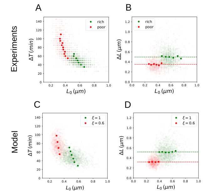
Figure 5: Comparison between experiments and model results. (A) Division time $\Delta T$ versus the cell size at birth $L_{0}$ from the mother machine experiment for rich and poor nutrient conditions. Each lighter dot represents a single cell cycle data. Darker dots are bin averages. (B) Elongation $\Delta L$ versus $L_{0}$ for the same experiments as in (A). (C,D) Same plots as (A) and (B) respectively, from numerical simulations of our model. The same $P_{d}(Z)$ as in Fig. 4 is used. See Sec. B for details on the simulations.

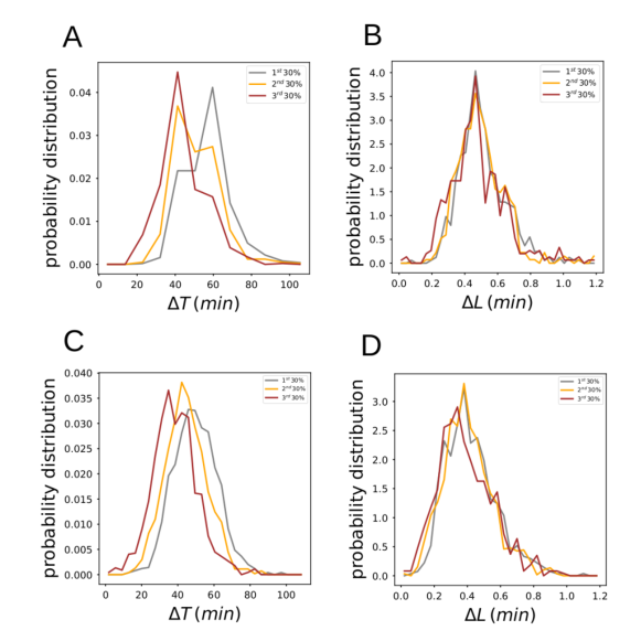
Figure 6: Conditional distributions in experiments and model. (A)&(B) The distributions of the division time ($\Delta T$) and the length elongation ($\Delta L$) when the size at birth $L_{0}$ is in three different percentiles from experimental measurements. The corresponding distributions from model results are shown in (C)&(D).

In Fig. 5A, the division time $\Delta T$ is plotted as a function of the size at birth $L_{0}$ for every cell cycle (lighter dots), together with the mean corresponding to a specific division time (darker dots), for two nutrient conditions from our mother machine experiments. Consistent with previous experiments [8], the size at birth has a negative correlation with respect to the division time, i.e., longer cells tend to divide faster. The mean value of the division time decreases for richer nutrient condition, suggesting that the rate of cell growth is influenced by the nutrient condition.

In Fig. 5B, values of $\Delta L$ for each generation are shown as a function of $L_{0}$ (lighter dots). It is clear from the mean values (darker dots) that the elongation $\Delta L$ does not depend on the initial size $L_{0}$, but it slightly increases when the nutrient conditions are richer. The independence of $\Delta L$ on $L_{0}$ is also consistent with previous experiments [8]. In fact, this empirical observation was incorporated into the phenomenological adder model [27, 38], which starts from the assumption that a cell divides when its elongation reaches a fixed value independent of its size at birth $L_{0}$. The negative correlation between $\Delta T$ and $L_{0}$ and the independence of $\Delta L$ on $L_{0}$ are the two key features in cell size control we wish to reproduce from our growth-division model.

In Fig. 5C, We show the division time $\Delta T$ versus the size at birth $L_{0}$ for each individual cell cycle (lighter dots) from our model. We divided the values of $L_{0}$ into equally spaced bins and calculated the average of $\Delta T$ and $L_{0}$ for each bin (darker dots). The same analysis was used to plot the increment $\Delta L$ as a function of the size at birth $L_{0}$ for different cell cycles in Fig. 5D. Our model reproduces the negative correlation between $L_{0}$ and $\Delta T$ as well as the independence of $\Delta L$ on $L_{0}$. Furthermore, the dependence of $\Delta T$, $L_{0}$, and $\Delta L$ on the nutrient conditions are also in quantitative agreement with our mother machine experiments. Moreover, for a given nutrient condition, it is possible to appreciate the dependency of $\Delta T$ and $\Delta L$ on $L_{0}$ by considering the conditional probability distributions. In Fig. 6 we plot the distributions of $\Delta T$ and $\Delta L$ for cell cycles in which the initial length $L_{0}$ was in specific ranges. We can thus notice that while $\Delta T$ tends to decrease for larger $L_{0}$, the distributions of $\Delta L$ collapse, and the results from the simulations are in line with the ones from the experiments.

D Derivation of the Langevin equation for the concentration using a mean field approximation

In this section and the next one we will derive the differential equation of the probability distribution $P(c)$ and the relation between the mean and the variance of the protein concentration in our mean field model. To do so, we first write the time derivative of $c$ in terms of derivatives of $N$ and $L$:

$$\frac{dc}{dt}=\frac{1}{L}\frac{dN}{dt}-\frac{c}{L}\frac{dL}{dt}\,.$$ (14)

Using Eq. 2 and Eq. 3 in the main text, the Langevin equation becomes:

$$\frac{dc}{dt}=\hat{K}_{n}-\hat{K}_{l}\,c+c\sum_{i}^{n_{d}(t)}\left[\left(w_{i}^{(l)}-w_{i}^{(n)}\right)\delta(t-t_{i})\right]\,.$$ (15)

The two variables for the division term are

$$w_{i}^{(l)} =\frac{L_{a}}{L_{b}}\,,$$ (16)

$$w_{i}^{(n)} =\frac{N_{a}}{N_{b}}$$ (17)

where $L_{b}$, $N_{b}$, $L_{a}$ and $N_{a}$ are the values of the size and the protein number before and after the division respectively.

The difference $\delta w_{i}=w_{i}^{(l)}-w_{i}^{(n)}$ has the following properties:

$$\left<\delta w_{i}\right> =0\,,$$

$$\left<\delta w_{i}\delta w_{j}\right> =2\Delta_{w}\delta_{ij}\,,$$ (18)

where $\Delta_{w}$ is the variance of the partition difference. We can thus define the noise due to cell division:

$$\eta_{d}(t)\equiv\sum_{i}^{n_{d}(t)}\delta w_{i}\delta(t-t_{i}(Z))\,.$$ (19)

This new stochastic variable has still mean equal to zero and it is delta-function correlated:

$$\left<\eta_{d}(t)\right>=0\,,$$ (20)

and

$$\left<\eta_{d}(t_{1})\eta_{d}(t_{2})\right>=2\Delta_{d}\delta(t_{2}-t_{1})\,,$$ (21)

where

$$\Delta_{d}=\frac{1}{2\left<\Delta T\right>}\left<\left(\frac{L_{a}}{L_{b}}-\frac{N_{a}}{N_{b}}\right)^{2}\right>\,.$$ (22)

The other sources of noise are discussed in F.

E Derivation of the square Taylor’s law

From the Langevin equation (Eq. 7 in the main text), the steady state protein concentration distribution function $P(c)$ satisfies the stationary Fokker-Planck equation:

$$\left<\hat{K}_{l}\right>\frac{d}{dc}\left[(\mu-c)P\right]=\frac{d^{2}}{dc^{2}}\left[D(c)P\right]\,,$$ (23)

where $D(c)=\mu^{2}\Delta_{a}+2\mu c\Delta_{am}+c^{2}\Delta_{m}$ with $\Delta_{(a,m,am)}$ representing the noise strength for $\eta_{a}$, $\eta_{m}$, and their correlation. The solution of Eq. 23 is reported in the main text (Eq. 11). Here we derive the relation between the mean and the variance.

After a first integration over $c$ we obtain

$$\left<\hat{K}_{l}\right>\left[(\mu-c)P(c)\right]=\frac{d}{dc}\left[D(c)P(c)\right]\,.$$ (24)

If we integrate on both sides and we use the fact that $P(c)D(c)\to 0$ when $c\to\infty$ we have

$$\left<\hat{K}_{l}\right>(\mu-\left<c\right>)=0\,,$$ (25)

and thus $\left<c\right>=\mu$. If instead we multiply Eq. 24 on both sides for $(\mu-c)/\left<\hat{K}_{l}\right>$, and we integrate over $c$, on the left hand side we simply have $\sigma_{c}^{2}$. Therefore, after an integration by parts, the equation reduces to

$$\sigma_{c}^{2}=\frac{1}{\left<\hat{K}_{l}\right>}\int D(c)P(c)dc=\frac{1}{\left<\hat{K}_{l}\right>}(\mu^{2}\Delta_{a}+2\mu^{2}\Delta_{am}+(\mu^{2}+\sigma_{c}^{2})\Delta_{m})\,.$$ (26)

By solving Eq. 26 we obtain the variance as a function of the noise strengths and $\mu$

$$\sigma_{c}^{2}=\frac{\Delta_{a}+2\Delta_{am}+\Delta_{m}}{\left<\hat{K}_{l}\right>-\Delta_{m}}\mu^{2}=\frac{\Delta_{d}+\Delta_{g}}{\left<\hat{K}_{l}\right>-\Delta_{m}}\mu^{2}\,,$$ (27)

where $\Delta_{a}=\left<\hat{K}_{l}\right>^{2}(\Delta_{(r)}+\Delta_{n})$ is the noise strength for $\eta_{a}$, $\Delta_{am}=-\left<\hat{K}_{l}\right>^{2}\Delta_{(r)}$ is the correlation between $\eta_{a}$ and $\eta_{m}$, and $\Delta_{m}=\Delta_{d}+\left<\hat{K}_{l}\right>^{2}(\Delta_{(r)}+\Delta_{l})$ is the strength of the noise $\eta_{m}$ with $\Delta_{(r)}=\langle\delta r^{2}\rangle/\langle r\rangle^{2}$ the noise strength for $\delta r/\langle r\rangle$. The above equation (Eq. 27) is the same as Eq. 10 in the main text.

F Detailed noise analysis

The averages of the effective growth and expression rates $\left<\hat{K}_{l,n}\right>$ can be calculated from experiments in the following way:

$$\left<\hat{K}_{l}\right> =\left<\frac{1}{L}\frac{\delta L}{\delta t}\right>\,,$$

$$\left<\hat{K}_{n}\right> =\left<\frac{1}{L}\frac{\delta N}{\delta t}\right>\,,$$ (28)

where $\delta L$, $\delta N$ and $\delta t$ are the smallest increment allowed by the experimental set up. In our case, the time step was $\delta t=5\,\mbox{min}$. From the experiments we do not have direct information about $R$ and the noise from the observable variables includes contributions from $r$ and contributions from $N$ and $L$. In other words, we can directly measure $\chi_{l}$ and $\chi_{n}$ but not $\eta_{l}$ and $\eta_{n}$. The noise strengths of $\chi_{l}$ and $\chi_{n}$ are given by the following formula:

$$\Delta_{(\chi_{l},\chi_{n})}=\frac{1}{2}\int ds\,\left<\chi_{(l,n)}(t)\chi_{(l,n)}(t+s)\right>\,.$$ (29)

Here the average is over an ensemble of time traces and the result will not depend on the specific time $t$.

Since the noises $\eta_{n}$ and $\eta_{l}$ are independent, when we calculate the correlation between $\chi_{l}$ and $\chi_{n}$ we obtain the strength of the noise $\delta r/\left<r\right>$ -the only non zero term in the correlation- that we call $\Delta_{(r)}$ (not to be confused with the strength of $\eta_{r}$) :

$$\Delta_{(r)}=\frac{1}{2}\int\,ds\,\left<\chi_{l}(t)\chi_{n}(t+s)\right>\,.$$ (30)

Once we have $\Delta_{(r)}$, by subtracting it from $\Delta_{\chi_{l}}$ and $\Delta_{\chi_{n}}$ we will obtain $\Delta_{l}$ and $\Delta_{n}$ respectively.

conditions	$\Delta_{\chi_{l}}$ (min)	$\Delta_{\chi_{n}}$ (min)	$\left<K_{l}\right>\,(\mbox{min}^{-1})$	$\Delta_{(r)}$ (min)	$\Delta_{m}\,(\mbox{min}^{-1})$	$\Delta_{d}\,(\mbox{min}^{-1})$	$\Delta_{g}/\Delta_{d}$	$A$
Rich 4	0.619	2.4	0.017	0.66	0.00023	5.5e-05	8.7	0.032
Rich 5	0.412	2.8	0.017	0.12	0.00015	3.7e-05	22	0.053
Rich B	0.429	1.7	0.017	0.56	0.00017	4.5e-05	6.8	0.021
Rich C	0.654	2.3	0.016	0.63	0.0002	3.7e-05	12	0.03
Rich D	0.904	1.8	0.015	0.85	0.00022	3e-05	6.9	0.017
Poor 4	9.42	8.5	0.0075	5.3	0.00057	3.9e-05	11	0.065
Poor 5	8.2	6.25	0.0092	4.3	0.00074	3.9e-05	12	0.063
Poor B	8.2	5.15	0.0087	3.5	0.00063	2.5e-05	22	0.061
Poor C	4.7	4.1	0.0092	2.2	0.00042	2.1e-05	18	0.045
Poor D	5.49	6.3	0.0087	3.4	0.00044	1.9e-05	19	0.048

Table 2: Relevant parameters inferred from the experiments for different promoter strengths and nutrient conditions. These values have been calculated by means of averages over different mother cells.

We can now write $\Delta_{a}$, $\Delta_{am}$ and $\Delta_{m}$ in terms of these noise strengths:

$$\Delta_{a} =\left<\hat{K}_{l}\right>^{2}\Delta_{\chi_{n}}\,,$$

$$\Delta_{m} =\Delta_{d}+\left<\hat{K}_{l}\right>^{2}\Delta_{\chi_{l}}\,,$$

$$\Delta_{am} =-\left<\hat{K}_{l}\right>^{2}\Delta_{(r)}$$

Given these expressions, the parameter $A$ can be written as

$$A=\frac{\Delta_{g}+\Delta_{d}}{\left<\hat{K}_{l}\right>-\Delta_{m}}\,,$$ (31)

where we have defined the growth noise strength:

$$\Delta_{g}=\left<\hat{K}_{l}\right>^{2}(\Delta_{\chi_{n}}+\Delta_{\chi_{l}}-2\Delta_{(r)})$$ (32)

In Fig. 7A we show the average coefficient $A$ for all the different conditions and promoter strengths. In Fig. 7B the distributions of $A$ are shown for the two nutrient conditions, sampling together the values of the mother cells for all promoter strengths. The noise strengths and other relevant parameters relative to all combinations of nutrient conditions and promoter strengths are reported in Table 2.

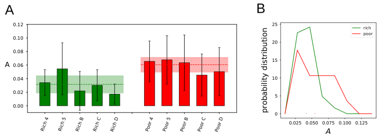
Figure 7: (A) Scaling prefactor constant $A$ averaged over all mother cells within a population with different combinations of nutrient conditions and promoter strengths. The dashed line indicates the average for a specific nutrient condition. The colored region indicates the standard deviation of the mean for each nutrient condition. (B) Distribution of $A$ from individual mother cells in rich and poor media.

References

- [1] Stefano Di Talia, Jan M. Skotheim, James M. Bean, Eric D. Siggia, and Frederick R. Cross. The effects of molecular noise and size control on variability in the budding yeast cell cycle. Nature, 448:947–951, 2007.
- [2] Avigdor Eldar and Michael B. Elowitz. Functional roles for noise in genetic circuits. Nature, 467:167–173, 2010.
- [3] Jie Lin and Ariel Amir. Homeostasis of protein and mrna concentrations in growing cells. Nature Communications, 9:4496, 2018.
- [4] Naama Brenner, Errez Braun, Anna Yoney, Lee Susman, James Rotella, and Hanna Salman. Single-cell protein dynamics reproduce universal fluctuations in cell populations. The European Physical Journal E, 38(9):102, 2015.
- [5] Zhixing Cao and Ramon Grima. Analytical distributions for detailed models of stochastic gene expression in eukaryotic cells. Proceedings of the National Academy of Sciences, 117(9):4682–4692, 2020.
- [6] Lee Susman, Maryam Kohram, Harsh Vashistha, Jeffrey T. Nechleba, Hanna Salman, and Naama Brenner. Individuality and slow dynamics in bacterial growth homeostasis. Proceedings of the National Academy of Sciences, 115(25):E5679–E5687, 2018.
- [7] Mats Wallden, David Fange, Ebba Gregorsson Lundius, Ozden Baltekin, and Johan Elf. The synchronization of replication and division cycles in individual e. coli cells. Cell, 166:729–739, 2016.
- [8] Sattar Taheri-Araghi, Serena Bradde, John T. Sauls, Norbert S. Hill, Petra Anne Levin, Johan Paulsson, Massimo Vergassola, and Suckjoon Jun. Cell-size control and homeostasis in bacteria. Current Biology, 25:385–391, 2015.
- [9] Yu Tanouchi, Anand Pai, Heungwon Park, Shuqiang Huang, Rumen Stamatov, Nicolas E. Buchler, and Lingchong You. A noisy linear map underlies oscillations in cell size and gene expression in bacteria. Nature, 523:357–360, 2015.
- [10] Alberto S. Sassi, Mayra Garcia-Alcala, Mark J. Kim, Philippe Cluzel, and Yuhai Tu. Filtering input fluctuations in intensity and in time underlies stochastic transcriptional pulses without feedback. Proceedings of the National Academy of Sciences, 2020.
- [11] Dann Huh and Johan Paulsson. Non-genetic heterogeneity from stochastic partitioning at cell division. Nature Genetics, 43:95–100, 2011.
- [12] J. Mark Kim, M. Garcia-Alcala, E. Balleza, and P. Cluzel. Stochastic transcriptional pulses orchestrate flagellum biosynthesis in E. coli. Sci. Adv., 6, Feb 2020.
- [13] John R S Newman, Sina Ghaemmaghami, Jan Ihmels, David K Breslow, Matthew Noble, Joseph L DeRisi, and Jonathan S Weissman. Single-cell proteomic analysis of s. cerevisiae reveals the architecture of biological noise. Nature, 441:840–846, 2006.
- [14] I. Soifer, L. Robert, and A. Amir. Single-cell analysis of growth in budding yeast and bacteria reveals a common size regulation strategy. Current Biology, 26(3):356–361, 2016.
- [15] Ping Wang, Lydia Robert, James Pelletier, Wei Lien Dang, Francois Taddei, Andrew Wright, and Suckjoon Jun. Robust growth of escherichia coli. Current Biology, 20(12):1099 – 1103, 2010.
- [16] Jean Ollion, Marina Elez, and Lydia Robert. High-throughput detection and tracking of cells and intracellular spots in mother machine experiments. Nature Protocols, 14(11):3144–3161, 2019.
- [17] Lionel R. Taylor. Aggregation, variance and the mean. Nature, 189:732–735, 1961.
- [18] Joel Cohen. Species-abundance distributions and taylor’s power law of fluctuation scaling. Theoretical Ecology, 13, 12 2020.
- [19] Meng Xu and Joel E. Cohen. Spatial and temporal autocorrelations affect taylor’s law for us county populations: Descriptive and predictive models. PloS ONE, 16(1):1–21, 01 2021.
- [20] Matt Keeling and Bryan Grenfell. Stochastic dynamics and a power law for measles. Phil. Trans. R. Soc. Lond. B., 354:769–776, 1999.
- [21] Joel E. Cohen. Taylor’s power law of fluctuation scaling and the growth-rate theorem. Theoretical Population Biology, 88:94–100, 2013.
- [22] Hanna Salman, Naama Brenner, Chih-kuan Tung, Noa Elyahu, Elad Stolovicki, Lindsay Moore, Albert Libchaber, and Erez Braun. Universal protein fluctuations in populations of microorganisms. Physical Review Letter, 108:238105, June 2012.
- [23] Naama Brenner, C. M. Newman, Dino Osmanović, Yitzhak Rabin, Hanna Salman, and D. L. Stein. Universal protein distributions in a model of cell growth and division. Phys. Rev. E, 92:042713, Oct 2015.
- [24] R.C. Lewontin and D. Cohen. On population growth in a randomly varying environment. Proceedings of the National Academy of Sciences, 62(4):1056–60, 1969.
- [25] Joel E. Cohen, Meng Xu, and William S. F. Schuster. Stochastic multiplicative population growth predicts and interprets taylor’s power law of fluctuation scaling. Proceedings of the Royal Society B: Biological Sciences, 280(1757):20122955, 2013.
- [26] Joel E. Cohen. Stochastic population dynamics in a markovian environment implies taylor’s power law of fluctuation scaling. Theoretical Population Biology, 93:30–37, 2014.
- [27] Ariel Amir. Cell size regulation in bacteria. Phys. Rev. Lett., 112:208102, May 2014.
- [28] P.A. Fantes, W.D. Grant, R.H. Pritchard, P.E. Sudbery, and A.E. Wheals. The regulation of cell size and the control of mitosis. Journal of Theoretical Biology, 50(1):213–244, 1975.
- [29] S. Wold, K. Skarstad, H.B. Steen, T. Stokke, and E. Boye. The initiation mass for dna replication in escherichia coli k-12 is dependent on growth rate. The EMBO Journal, 13(9):2097–2102, 1994.
- [30] Erik Boye and Kurt Nordström. Coupling the cell cycle to cell growth. EMBO reports, 4(8):757–760, 2003.
- [31] William D Donachie and Garry W Blakely. Coupling the initiation of chromosome replication to cell size in escherichia coli. Current Opinion in Microbiology, 6(2):146–150, 2003.
- [32] Markus Basan, Manlu Zhu, Xiongfeng Dai, Mya Warren, Daniel Sévin, Yi-Ping Wang, and Terence Hwa. Inflating bacterial cells by increased protein synthesis. Molecular Systems Biology, 11(10):836, 2015.
- [33] Joseph H. Davis, Adam J. Rubin, and Robert T. Sauer. Design, construction and characterization of a set of insulated bacterial promoters. Nucleic Acids Research, 39(3):1131–1141, 2011.
- [34] Matthew Scott, Carl W. Gunderson, Eduard M. Mateescu, Zhongge Zhang, and Terence Hwa. Interdependence of cell growth and gene expression: Origins and consequences. Science, 330(6007):1099–1102, 2010.
- [35] Fangwei Si, Guillaume Le Treut, John T. Sauls, Stephen Vadia, Petra Anne Levin, and Suckjoon Jun. Mechanistic origin of cell-size control and homeostasis in bacteria. Current Biology, 29:1760–1770, 2019.
- [36] K Dai and J Lutkenhaus. ftsz is an essential cell division gene in escherichia coli. Journal of Bacteriology, 173(11):3500–3506, 1991.
- [37] A Mukherjee, K Dai, and J Lutkenhaus. Escherichia coli cell division protein ftsz is a guanine nucleotide binding protein. Proceedings of the National Academy of Sciences, 90(3):1053–1057, 1993.
- [38] Lisa Willis and Kerwyn Casey Huang. Sizing up the bacterial cell cycle. Nature Reviews Microbiology, 15:606–620, Aug 2017.
- [39] François Bertaux, Julius von Kügelgen, Samuel Marguerat, and Vahid Shahrezaei. A bacterial size law revealed by a coarse-grained model of cell physiology. PLOS Computational Biology, 16(9):1–21, 09 2020.
- [40] Zoltán Eisler, Imre Bartos, and János Kertész. Fluctuation scaling in complex systems: Taylor’s law and beyond. Advances in Physics, 57(1):89–142, 2008.