Taming the pinch singularities in the two-loop neutrino self-energy in a medium

Abstract

We consider the calculation of the thermal self-energy of a neutrino that propagates in a medium composed of fermions and scalars interacting via a Yukawa-type coupling, in the case that the neutrino energy is much larger than the fermion and scalar masses, as well as the temperature and chemical potentials of the background. In this kinematic regime the one-loop contribution to the imaginary part of the self-energy is negligible. We consider the two-loop contribution and we encounter the so-called pinch singularities which are known to arise in higher loop self-energy calculations in Thermal Field Theory. With a judicious use of the properties and parametrizations of the thermal propagators the singularities are treated effectively and actually disappear. From the imaginary part of the self-energy, we obtain a precise formula for the damping matrix expressed in terms of integrals over the background particle distributions. The formulas predict a specific dependence of the damping terms on the neutrino energy, depending on the background conditions. For guidance in estimating the effects in specific contexts, we compute the damping terms for several limiting cases of the momentum distribution functions of the background particles. We discuss briefly the connection between the results of our calculations for the damping matrix and the decoherence effects described in terms of the Lindblad equation.

1 Introduction and Summary

In several models and extensions of the standard electro-weak theory the neutrinos interact with scalar particles ($\phi$) and fermions ($f$) via a coupling of the form

$$L_{int}=\sum_{a}g_{a}\bar{f}_{R}\nu_{La}\phi+h.c\,.$$ (1.1)

For definiteness we are assuming the presence of only one $f$ and $\phi$, while the indices $a,b,c,...$ label the neutrino flavors. Those interactions produce nonstandard contributions to the neutrino index of refraction and effective potential when the neutrino propagates in a background of those particles. Couplings of this form have been considered recently in the context of Dark Matter-neutrino interactions[1, 2, 3, 4, 5, 6, 7, 8, 9]. Similar effects occur due to neutrino-neutrino-scalar interactions of the form $\bar{\nu}^{c}_{Rb}\nu_{La}\phi$ when a neutrino propagates in a neutrino background. This can occur in the environment of a supernova, where the neutrino-neutrino interactions lead to the collective neutrino oscillations and related phenomena (see for example Refs. [10] and [11] and the works cited therein), and it can also occur in the hot plasma of the Early Universe before the neutrinos decouple[12, 13].

In previous works we have presented various calculations related to the propagation of neutrinos in that kind of background[14, 15, 16]. In Ref. [14] we considered the real part of the self-energy of a neutrino that propagates in a medium consisting of fermions and scalars, with a coupling of the form given in Eq. (1.1). We calculated the real part (or more precisely the dispersive part) of the neutrino thermal self-energy, denoted by $\Sigma_{r}$, from which the dispersion relation and effective potential are determined. Those interactions can also induce processes such as $\nu+\phi\leftrightarrow f$ and $\nu+\bar{f}\leftrightarrow\bar{\phi}$, depending on the kinematic conditions, that produce damping terms in the neutrino dispersion relation and index of refraction. Thus in Ref. [15], we continued our work to calculate the imaginary part (or more precisely the absorptive part) of the neutrino thermal self-energy, denoted by $\Sigma_{i}$, in a scalar and fermion background due to the $\bar{f}_{R}\nu_{L}\phi$ interaction. From $\Sigma_{i}$ the corresponding contribution to the damping matrix $\Gamma$ in the dispersion relation were obtained. The calculations in Ref. [15] were based on the one-loop diagram for the neutrino self-energy.

In Ref. [16] we noted that those couplings can induce decoherence effects, of the form discussed in recent works [17, 18, 19, 20, 21], due to the neutrino non-forward scattering process $\nu_{a}+x\rightarrow\nu_{b}+x$, where $x=f,\phi$. As observed in Ref. [16], the contribution to $\Gamma$ due to these processes can be determined from the two-loop calculation of $\Sigma_{i}$. Thus, in that reference we performed the two-loop calculation of $\Sigma_{i}$ and $\Gamma$ or the case in which the background contains only the fermions $f$, assuming that the $\phi$ particle is heavy enough and the conditions are such that there are no $\phi$ particles in the background. Under those conditions, the two-loop contribution to $\Gamma$ is the relevant one since the two-body processes that contribute in one-loop are kinematically forbidden.

The present work is a continuation of that previous work. Here we consider the situation in which both $f$ and $\phi$ may be present in the background. We are particularly interested in the kinematic regime

$$\kappa>m_{\phi},m_{f},T\,,$$ (1.2)

where $\kappa$ is the neutrino momentum and $T$ the background temperature. That is, both $f$ and $\phi$ are relatively light compared to the neutrino energy. We refer to this as the light background. It is the kinematic regime that is relevant in the context of the possible existence of light scalars as dark-matter and the effects they may have on neutrino experiments, that has been explored in the recent literature[22, 23]. The results can be useful also for the studies of the environmental decoherence effects in long baseline neutrino oscillation experiments that have been carried out recently[24, 25, 26, 27]. Again, in this kinematic regime the two-body processes that contribute in one-loop are inhibited and the two-loop contribution is the relevant one.

Apart from the relevance for the applications already mentioned, from a calculational point of view the present calculation has a technical merit. There is one important technical issue that shows up in the kinematic regime we are considering in the present case and those we considered previously. The two-loop diagrams for the self-energy, from which the damping matrix is determined, suffer from the so-called pinch-singularities[28]. These arise from the fact that in the present case some of the diagrams contain a product of two thermal propagators with the same momentum. Since the thermal propagators involve the on-shell delta functions, such products are ill-defined. As we show, by a judicious use of the properties and parametrizations of the thermal propagators, the expressions for the diagrams can be rearranged such that the pinch singularities are absent in the final expressions, allowing a straightforward evaluation of the self-energy and whence the damping terms. While the conventional wisdom is that indeed such singularities actually disappear, our calculations provide an explicit proof of that fact in a concrete and non-trivial example that can be generalized to other calculations.

The final results are well defined formulas for the damping terms in the neutrino dispersion relation (or effective potential) in terms of the model parameters (i.e., couplings $g_{a}$, masses $m_{f,\phi}$) and the enviromental parameters (e.g. temperature). In practical applications, the possible values of all the parameters involved vary significantly depending on the context, i.e., astrophysical, cosmological or neutrino oscillations. For example, in the context of a supernova (such as SN1987A) the neutrino interactions with $\phi$ as a cold dark matter candidate can have effects on the observed neutrino flux for $m_{\phi},T\sim\mbox{a few}$ MeV[1]. But these, and similar considerations in other contexts, depend on the particle physics model as well. Thus, for example, while we concentrate here on the calculation involving the $L_{int}$ interaction term, in isolation from the Standard Model interactions, the two-loop diagrams in some models may involve the standard particles and/or other non-standard gauge boson interactions as well. Nevertheless, subject to the limitation of the light background condition stated above, the particular results we obtain for the damping terms can be used in the context of many such models and conditions, and in fact the method to treat the pinch singularities is applicable to those more general cases as well.

In summary, our plan is as follows. In Section 2 we summarize the framework in which we carry out the calculations. There we explain that, while the effective potential is determined from the one-loop diagram for the self-energy, in the kinematic regime we consider [Eq. (1.2)] the damping is determined form the two-loop diagrams. In Section 3 we calculate the dispersive part of the self-energy and determine the effective potential. In Section 4 we consider the calculation of the two-loop contribution to the absorptive part of the self-energy, from which the damping matrix is determined. There we indicate the problem of the pinch singularities, and present our treatment to resolve it. The net result, summarized in Section 4.4, is the set of formulas for the two-loop contributions to the absorptive part of the self-energy, free from the singularities. In Section 5 we evaluate explicitly the corresponding expressions for the damping matrix in the case of a scalar background under various conditions, and indicate the path to generalize such calculations to consider more complicated backgrounds. There we also discuss briefly the connection between the damping matrix thus determined and the decoherence described in terms of the Lindblad equation. Finally Section 6 has our conclusions.

2 Preliminaries - effective potential and the damping matrix

To be self-contained we summarize the following material borrowing from Ref. [16]. We denote by $k^{\mu}$ the momentum four-vector of the propagating neutrino, and as usual we denote by $u^{\mu}$ the velocity four-vector of the background medium. In the background medium’s own rest frame, it takes the form

$$u^{\mu}=(1,\vec{0})\,,$$ (2.1)

and in this frame we write

$$k^{\mu}=(\omega,\vec{\kappa})\,.$$ (2.2)

Since we are considering only one background medium, it can be taken to be at rest and therefore we adopt Eqs. (2.1) and (2.2) throughout.

Let us consider first the case of one neutrino propagating in the medium. The dispersion relation and the spinor of the propagating mode are determined by solving the equation

$$\left(k\hbox to0.0pt{\hss/}-\Sigma_{eff}\right)\psi_{L}(k)=0\,,$$ (2.3)

where $\Sigma_{eff}$ is the neutrino thermal self-energy. It can be decomposed in the form

$$\Sigma_{eff}=\Sigma_{r}+i\Sigma_{i}\,,$$ (2.4)

where $\Sigma_{r,i}$ are the dispersive and absorptive parts,

$$\Sigma_{r} = \frac{1}{2}\left(\Sigma_{eff}+\bar{\Sigma}_{eff}\right)\,,$$

$$\Sigma_{i} = \frac{1}{2i}\left(\Sigma_{eff}-\bar{\Sigma}_{eff}\right)\,,$$ (2.5)

respectively, with

$$\bar{\Sigma}_{eff}=\gamma^{0}\Sigma^{\dagger}_{eff}\gamma^{0}\,.$$ (2.6)

In the context of thermal field theory $\Sigma_{r}$ is given in terms of the $11$ element of the thermal self-energy matrix by

$$\Sigma_{r}=\Sigma_{11r}\equiv\frac{1}{2}(\Sigma_{11}+\overline{\Sigma}_{11})\,.$$ (2.7)

On the other hand, $\Sigma_{i}$ is more conveniently determined in terms of the $12$ element of the neutrino thermal self-energy matrix by the formula

$$\Sigma_{i}=\frac{\Sigma_{12}}{2in_{F}(x_{\nu})}\,.$$ (2.8)

Here

$$n_{F}(z)=\frac{1}{e^{z}+1}\,,$$ (2.9)

is the fermion distribution function, written in terms of a dummy variable $z$, and the variable $x_{\nu}(k)$ is given by

$$x_{\nu}(k)=\beta k\cdot u-\alpha_{\nu}\,,$$ (2.10)

where $T=1/\beta$ is the temperature and $\alpha_{\nu}$ is the neutrino chemical potential.

The chirality of the neutrino interactions imply that

$$\Sigma_{eff}=V^{\mu}\gamma_{\mu}L\,.$$ (2.11)

Here and below we use the notation $L$ and $R$ for the left and right chiral projection matrices $L,R=\frac{1}{2}(1\mp\gamma_{5})$, respectively. Corresponding to the decomposition in Eq. (2.4) we also write

$$V^{\mu}=V^{\mu}_{r}+iV^{\mu}_{i}\,.$$ (2.12)

and

$$\Sigma_{r,i}=V^{\mu}_{r,i}\gamma_{\mu}L\,.$$ (2.13)

In general $V^{\mu}_{r,i}$ are functions of $\omega$ and $\vec{\kappa}$. We omit those arguments ordinarily but we will restore them when needed.

Writing the neutrino and antineutrino dispersion relations in the form

$$\omega^{(\nu,\bar{\nu})}(\kappa)=\omega^{(\nu,\bar{\nu})}_{r}(\kappa)-\frac{i\gamma^{(\nu,\bar{\nu})}(\kappa)}{2}\,,$$ (2.14)

the solution of Eq. (2.3) gives

$$\omega^{(\nu,\bar{\nu})}_{r}=\kappa+V^{(\nu,\bar{\nu})}_{eff}$$ (2.15)

where $V^{(\nu,\bar{\nu})}_{eff}$ are the effective potentials

$$V^{(\nu)}_{eff} = n\cdot V_{r}(\kappa,\vec{\kappa})=V^{0}_{r}(\kappa,\vec{\kappa})-\hat{\kappa}\cdot\vec{V}_{r}(\kappa,\vec{\kappa})\,,$$

$$V^{(\bar{\nu})}_{eff} = -n\cdot V_{r}(-\kappa,-\vec{\kappa})=-V^{0}_{r}(-\kappa,-\vec{\kappa})+\hat{\kappa}\cdot\vec{V}_{r}(-\kappa,-\vec{\kappa})\,,$$ (2.16)

with

$$n^{\mu}=(1,\hat{\kappa})\,.$$ (2.17)

On the other hand, for the imaginary part,

$$-\frac{\gamma^{(\nu)}(\vec{\kappa})}{2} = \frac{n\cdot V_{i}(\kappa,\vec{\kappa})}{1-n\cdot\left.\frac{\partial V_{r}(\omega,\vec{\kappa})}{\partial\omega}\right|_{\omega=\kappa}}\,,$$

$$-\frac{\gamma^{(\bar{\nu})}(\vec{\kappa})}{2} = \frac{n\cdot V_{i}(-\kappa,-\vec{\kappa})}{1-n\cdot\left.\frac{\partial V_{r}(\omega,-\vec{\kappa})}{\partial\omega}\right|_{\omega=-\kappa}}\,,$$ (2.18)

where $n^{\mu}$ is defined in Eq. (2.17). We will retain only the dominant contribution to $n\cdot V_{i}$ in the numerator, which in our case is the two-loop term as we argue below. Then to leading order the formulas in Eq. (2) reduce to

$$-\frac{\gamma^{(\nu)}(\vec{\kappa})}{2} = n\cdot V_{i}(\kappa,\vec{\kappa})\,,$$

$$-\frac{\gamma^{(\bar{\nu})}(\vec{\kappa})}{2} = n\cdot V_{i}(-\kappa,-\vec{\kappa})\,.$$ (2.19)

neglecting the correction due to the $n\cdot\partial V_{r}(\omega,\vec{\kappa})/\partial\omega$ term in the denominator.

In the case of various neutrino flavors, the vector $V^{\mu}$ in Eq. (2.11) is a matrix in the neutrino flavor space. As shown in Ref. [16], the generalization of the above discussion is that the dispersion relations of the propagating modes are determined by solving the following eigenvalue equation in flavor-space,

$$\left(H_{r}-i\frac{\Gamma}{2}\right)\xi=\omega\xi\,,$$ (2.20)

where $H_{r}$ and $\Gamma$ are Hermitian matrices in flavor space given by

$$H_{r} = \left\{\begin{array}[]{ll}\kappa+n\cdot V_{r}(\kappa,\vec{\kappa})&(\nu)\\ \kappa-n\cdot V^{\ast}_{r}(-\kappa,-\vec{\kappa})&(\bar{\nu})\,,\end{array}\right.$$ (2.23)

$$-\frac{1}{2}\Gamma = \left\{\begin{array}[]{ll}n\cdot V_{i}(\kappa,\vec{\kappa})&(\nu)\\ n\cdot V^{\ast}_{i}(-\kappa,-\vec{\kappa})&(\bar{\nu})\,.\end{array}\right.$$ (2.26)

In coordinate space, this translates to the evolution equation

$$i\partial_{t}\xi(t)=\left(H_{r}-i\frac{\Gamma}{2}\right)\xi(t)\,.$$ (2.27)

We refer to $\Gamma$ as the damping matrix, and to its elements as the damping terms. Our purpose in this work is to determine the contribution to $H_{r}$, and specially $\Gamma$, due to the presence of the light background.

The lowest order diagram is shown in Fig. 1. From that diagram we obtain $\Sigma_{11}$ and $\Sigma_{12}$, and whence the dispersive and absorptive parts $\Sigma_{r,i}$ by means of Eqs. (2.7) and (2.8). The corresponding one-loop contribution to $V_{r}$ and $\Gamma$ are then obtained from Eq. (2.23).

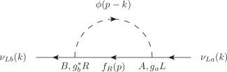
Figure 1: One-loop diagram for the neutrino self-energy matrix $(\Sigma_{AB})_{ba}$ in a background of fermions $f$ and scalars $\phi$. $a,b$ are neutrino flavor indices while $A$ and $B$ label the thermal vertices, that can take the values 1 or 2.

However, as in the cases discussed in Refs. [16] and [29], the one-loop contribution to $\Sigma_{12}$ is negligible in this case also. The reason is that such contributions arise from the two-body neutrino processes such as $\nu+\phi\leftrightarrow f$, which are inhibited by the kinematics in the regime we are considering [i.e, Eq. (1.2)].

To be more specific, the one-loop damping term is due to real processes like

$$(A) \nu+\bar{f} \leftrightarrow\bar{\phi}\quad\mbox{(if $m_{\phi}>m_{f}$)}$$

$$(B) \nu+\phi \leftrightarrow f\quad\mbox{(if $m_{f}>m_{\phi}$)}\,.$$ (2.28)

The calculation of the one-loop damping terms for all such conditions was carried out in Ref. [15]. Let us consider (A). As shown in that reference, the damping is maximum for values of the neutrino momentum

$$\kappa \sim \frac{m^{2}_{\phi}}{T}\quad\mbox{(if $T\gg m_{f}$)}$$

$$\kappa \sim \frac{m^{2}_{\phi}}{m_{f}}\quad\mbox{(if $T\ll m_{f}$)}\,.$$ (2.29)

Outside of those ranges the damping becomes exponentially small. Analogous considerations apply to case (B) as well. As a result, in the kinematic regime we are considering, the damping matrix is determined by the two-loop diagrams for $\Sigma_{12}$ shown in Fig. 2.

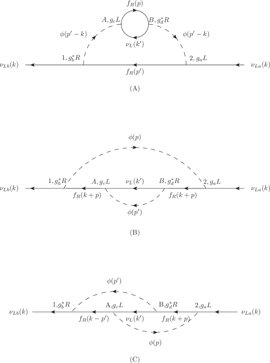
Figure 2: Two-loop diagram for the 12 element of the neutrino self-energy matrix in a background of fermions $f$ and scalars $\phi$, obtained by inserting additional propagators in the one-loop diagram in Fig. 1. The meaning of the labels $A,B$ are the same as in Fig. 1 while $a,b,c,d$ are neutrino flavor indices. To simplify the notation we are setting $k^{\prime}=k+p-p^{\prime}$. Diagram C does not exist if $\phi$ is a complex scalar field. For a real scalar diagram C must be included.

In summary, the neutrino and antineutrino effective potential is given by Eq. (2.16), and the damping by Eq. (2.19), where $V^{\mu}_{r}$ is determined from the calculation of $\Sigma_{11}$ using the one-loop diagram in Fig. 1, while $V^{\mu}_{i}$ is determined from $\Sigma_{12}$ calculated from the two-loop diagrams in Fig. 2. As already stated, in writing Eq. (2.19) we are neglecting the correction due to the $n\cdot\partial V_{r}(\omega,\vec{\kappa})/\partial\omega$ in the overall denominator in Eq (2.18), which corresponds to keep the leading order of the dominant term. As we have emphasized, the expressions corresponding to the diagrams in Fig. 2 suffer from the pinch singularities. After handling the singularities, $\Sigma_{12}$ is expressed in terms of integrals over the background particles distribution functions that can be evaluated in principle once the background conditions are specified. Correspondingly, the final formula for the damping matrix that we determine by means of Eq. (2.23) is expressed in terms of integrals over the background particle distribution functions that we will evaluate explicitly for some illustrative cases.

3 Effective potential

3.1 Dispersive part $\Sigma_{r}$

The contribution of the diagram in Fig. 1 to the 11 component of the neutrino thermal self-energy matrix is given by

$$-i(\Sigma_{11})_{ba}=\int\,\frac{d^{4}p}{(2\pi)^{4}}i\Delta^{(\phi)}_{11}(p-k)(ig^{\ast}_{b}R)iS^{(f)}_{11}(p)(ig_{a}L)\,.$$ (3.1)

We write the 11 components of the $f$ and $\phi$ thermal propagators in the form

$$iS^{(f)}_{11}(p) = (p\hbox to0.0pt{\hss/}+m_{f})\left[\frac{i}{p^{2}-m^{2}+i\epsilon}-2\pi\delta(p^{2}-m^{2}_{f})\eta_{f}(p)\right]\,,$$

$$i\Delta^{(\phi)}_{11}(p) = \frac{i}{p^{2}-m^{2}_{\phi}+i\epsilon}+2\pi\delta(p^{2}-m^{2}_{\phi})\eta_{\phi}(p)\,,$$ (3.2)

where

$$\eta_{f}(p) = n_{F}(x_{f}(p))\theta(p\cdot u)+n_{F}(-x_{f}(p))\theta(-p\cdot u)\,,$$

$$\eta_{\phi}(p) = n_{B}(x_{f}(p))\theta(p\cdot u)+n_{F}(-x_{f}(p))\theta(-p\cdot u)\,.$$ (3.3)

with $\theta$ being the unit step function. Here $n_{F}$ is the fermion momentum distribution function defined in Eq. (2.9), and $n_{B}$ is the corresponding one for bosons,

$$n_{B}(z)=\frac{1}{e^{z}-1}\,.$$ (3.4)

The variables $x_{f,\phi}$ are given by

$$x_{f}(p)=\beta p\cdot u-\alpha_{f}\,,$$

$$x_{\phi}(p)=\beta p\cdot u-\alpha_{\phi}\,,$$ (3.5)

where $\alpha_{f,\phi}$ are the chemical potentials. Discarding the pure vacuum contribution in Eq. (3.1) we then have

$$\Sigma_{r}=\Sigma^{(f)}_{r}+\Sigma^{(\phi)}_{r}\,,$$ (3.6)

where

$$\left(\Sigma^{(f)}_{r}\right)_{ba} = -g^{\ast}_{b}g_{a}\int\frac{d^{4}p}{(2\pi)^{3}}\frac{p\hbox to0.0pt{\hss/}L}{(p-k)^{2}-m^{2}_{\phi}}\delta(p^{2}-m^{2}_{f})\eta_{f}(p)\,,$$ (3.7)

$$\left(\Sigma^{(\phi)}_{r}\right)_{ba} = g^{\ast}_{b}g_{a}\int\frac{d^{4}p}{(2\pi)^{3}}\frac{(p\hbox to0.0pt{\hss/}+k\hbox to0.0pt{\hss/})L}{(p+k)^{2}-m^{2}_{f}}\delta(p^{2}-m^{2}_{\phi})\eta_{\phi}(p)\,.$$ (3.8)

3.2 Effective potential in the light background

For completeness and to make the present work self-contained, here we consider specifically the case of the light background in the sense of Eq. (1.2). In correspondence to Eq. (2.13), we write the $\Sigma^{(x)}_{r}$ ($x=f,\phi$) in the form

$$\Sigma^{(x)}_{r}=V^{(x)\mu}_{r}\gamma_{\mu}L\,,$$ (3.9)

and therefore

$$V^{\mu}_{r}=V^{(f)\mu}_{r}+V^{(\phi)\mu}_{r}\,.$$ (3.10)

From Eqs. (3.7) and (3.8) we then have

$$\left(V^{(f)\mu}_{r}(\omega,\kappa)\right)_{ba} = -(g^{\ast}_{b}g_{a})\int\frac{d^{4}p}{(2\pi)^{3}}\frac{p_{\mu}}{(p-k)^{2}-m^{2}_{\phi}}\delta(p^{2}-m^{2}_{f})\eta_{f}(p)\,,$$ (3.11)

$$\left(V^{(\phi)\mu}_{r}(\omega,\kappa)\right)_{ba} = (g^{\ast}_{b}g_{a})\int\frac{d^{4}p}{(2\pi)^{3}}\frac{(p^{\mu}+k^{\mu})}{(p+k)^{2}-m^{2}_{f}}\delta(p^{2}-m^{2}_{\phi})\eta_{\phi}(p)\,.$$ (3.12)

Under the conditions that we are considering [i.e., Eq. (1.2)], we can make the replacement

$$\frac{1}{(p+k)^{2}-m^{2}_{f}} \rightarrow \frac{1}{2p\cdot k+k^{2}}\,,$$

$$\frac{1}{(p-k)^{2}-m^{2}_{\phi}} \rightarrow \frac{-1}{2p\cdot k-k^{2}}\,,$$ (3.13)

in Eqs. (3.11) and (3.12). Furthermore, since the effective potential is defined by setting $\omega=\kappa$ [i.e., Eq. (2.23)], we can set

$$k^{\mu}=\kappa n^{\mu}\,,$$ (3.14)

where $n^{\mu}$ is defined in Eq. (2.17). Thus,

$$\left(V^{(f)\mu}_{r}(\kappa,\kappa)\right)_{ba} = (g^{\ast}_{b}g_{a})\int\frac{d^{4}p}{(2\pi)^{3}}\frac{p_{\mu}}{2p\cdot k}\delta(p^{2}-m^{2}_{f})\eta_{f}(p)\,,$$ (3.15)

$$\left(V^{(\phi)\mu}_{r}(\kappa,\kappa)\right)_{ba} = (g^{\ast}_{b}g_{a})\int\frac{d^{4}p}{(2\pi)^{3}}\frac{(p^{\mu}+\kappa n^{\mu})}{2p\cdot k}\delta(p^{2}-m^{2}_{\phi})\eta_{\phi}(p)\,.$$ (3.16)

Carrying out the integral over $p^{0}$ with the help of the delta function, we then have

$$\left(V^{(f)\mu}_{r}(\kappa,\vec{\kappa})\right)_{ba} = \frac{g^{\ast}_{b}g_{a}}{2\kappa}\int\frac{d^{3}p}{(2\pi)^{3}2E_{f}}\frac{p^{\mu}}{p\cdot n}\left[f_{f}(E_{f})+f_{\bar{f}}(E_{f})\right]\,,$$

$$\left(V^{(\phi)\mu}_{r}(\kappa,\vec{\kappa})\right)_{ba} = \frac{g^{\ast}_{b}g_{a}}{2\kappa}\int\frac{d^{3}p}{(2\pi)^{3}2E_{\phi}}\frac{1}{p\cdot n}\left\{p^{\mu}\left[f_{\phi}(E_{\phi})+f_{\bar{\phi}}(E_{\phi})\right]\right.$$ (3.17)

$$\mbox{}+\left.\kappa n^{\mu}\left[f_{\phi}(E_{\phi})-f_{\bar{\phi}}(E_{\phi})\right]\right\}\,,$$

and

$$V^{(x)\mu}_{r}(-\kappa,-\vec{\kappa})=\left.V^{(x)\mu}_{r}(\kappa,\vec{\kappa})\right|_{n^{\mu}\rightarrow-n^{\mu}}\,.$$ (3.18)

In Eq. (3.2) we have introduced the $f$ and $\phi$ momentum distribution functions (in the rest frame of the medium)

$$f_{f,\bar{f}}(E_{f}) = \frac{1}{e^{\beta E_{f}\mp\alpha_{f}}+1}\,,$$

$$f_{\phi,\bar{\phi}}(E_{\phi}) = \frac{1}{e^{\beta E_{\phi}\mp\alpha_{\phi}}-1}\,,$$ (3.19)

and it is understood that in each integral,

$$p^{\mu}=(E_{x},\vec{p})\qquad(x=f,\phi)\,,$$ (3.20)

with

$$E_{x}=\sqrt{{\vec{p}}{\,{}^{2}}+m^{2}_{x}}\,.$$ (3.21)

Thus remembering that $n^{2}=0$,

$$\left(n\cdot V^{(x)}(\kappa,\vec{\kappa})\right)_{ba}=-\left(n\cdot V^{(x)}(-\kappa,-\vec{\kappa})\right)_{ba}=\frac{g^{\ast}_{b}g_{a}}{2\kappa}\int\frac{d^{3}p}{(2\pi)^{3}2E_{x}}\left[f_{x}(E_{x})+f_{\bar{x}}(E_{x})\right]\,.$$ (3.22)

From Eq. (2), we then have

$$\left(V^{(\nu)}_{eff}(\vec{\kappa})\right)_{ba}=\left(V^{(\bar{\nu})}_{eff}(\vec{\kappa})\right)_{ba}=(V_{f})_{ba}+(V_{\phi})_{ba}\,,$$ (3.23)

where ($x=f,\phi$)

$$(V_{x})_{ba}=\frac{g^{\ast}_{b}g_{a}}{2\kappa}J_{x}\,,$$ (3.24)

and we have defined

$$J_{x}\equiv\int\frac{d^{3}p}{(2\pi)^{3}2E_{x}}\left[f_{x}(E_{x})+f_{\bar{x}}(E_{x})\right]\,.$$ (3.25)

Eqs. (3.23)-(3.25) reveal a number of differences in contrast with the Wolfenstein term that gives standard matter contribution to the effective potential[30]. The effective potential in this case is momentum-dependent, proportional to $1/\kappa$, has the same sign for neutrinos and antineutrinos, and does not vanish in a particle-antiparticle symmetric background. In fact, as is well known, for practical purposes the parameters $g^{\ast}_{b}g_{a}J_{f}$ and $g^{\ast}_{b}g_{a}J_{\phi}$ act as contributions to the vacuum squared mass matrix, with the same value (and sign) for neutrinos and antineutrinos (see e.g., Ref. [31]).

It is a simple matter to evaluate $J_{x}$ for different conditions of the background. For example, and for reference purposes, in the non-relativistic (NR) limit, or in the ultra-relativistic (UR) limit and zero chemical potential,

$$J_{\phi}=\left\{\begin{array}[]{ll}\frac{1}{2m_{\phi}}(n_{\phi}+n_{\bar{\phi}})&\mbox{(NR)}\\[12.0pt] \frac{T^{2}}{12}&\mbox{(UR)}\,,\end{array}\right.$$ (3.26)

and similarly for $J_{f}$. In Eq. (3.26), $n_{\phi,\bar{\phi}}$ are the total number densities of $\phi$ and $\bar{\phi}$, respectively, i.e.,

$$n_{\phi,\bar{\phi}}=\int\frac{d^{3}p}{(2\pi)^{3}}f_{\phi,\bar{\phi}}(E_{\phi})\,.$$ (3.27)

In Eq. (3.26) we have assumed that $\phi$ is complex. For a real $\phi$, in the NR limit

$$J_{\phi}=\frac{n_{\phi}}{m_{\phi}}\qquad\mbox{(NR)}\,.$$ (3.28)

In the UR limit the formula in Eq. (3.26) holds in this case as well.

4 Two-loop diagrams - absence of pinch singularities

We reiterate that we assume $\kappa$ to be high enough so that the conditions such as those given in Eq. (2) (or the analogous ones in case (B)) are satisfied and therefore the one-loop contribution to the damping matrix, arising from the two-body processes shown in Eq. (2) is negligible. As we have already mentioned, in that case the damping terms arise from the two-loop diagrams for $\Sigma_{12}$ shown in Fig. 2, which are obtained by inserting additional propagators in the one-loop diagram in Fig. 1. The corresponding expressions for their contributions to $\Sigma_{12}$ are

$$-i\left(\Sigma^{(A)}_{12}(k)\right)_{ba} = \sum_{A,B}\sum_{c,d}\int\frac{d^{4}p}{(2\pi)^{4}}\frac{d^{4}p^{\prime}}{(2\pi)^{4}}(i\eta_{1}g^{\ast}_{b}R)iS^{(f)}_{12}(p^{\prime})(i\eta_{2}g_{a}L)i\Delta^{(\phi)}_{2B}(p^{\prime}-k)i\Delta^{(\phi)}_{A1}(p^{\prime}-k)$$ (4.1)

$$\mbox{}\times(-1)\mbox{Tr}\left\{(i\eta_{A}g_{c}L)\left(iS^{(\nu)}_{AB}(k^{\prime})\right)_{cd}(i\eta_{B}g^{\ast}_{d}R)iS^{(f)}_{BA}(p)\right\}\,,$$

$$-i\left(\Sigma^{(B)}_{12}(k)\right)_{ba} = \sum_{A,B}\sum_{c,d}\int\frac{d^{4}p}{(2\pi)^{4}}\frac{d^{4}p^{\prime}}{(2\pi)^{4}}i\Delta^{(\phi)}_{21}(p)i\Delta^{(\phi)}_{AB}(p^{\prime})(i\eta_{1}g^{\ast}_{b}R)iS^{(f)}_{1A}(k+p)(i\eta_{A}g_{c}L)$$ (4.2)

$$\mbox{}\times\left(iS^{(\nu)}_{AB}(k^{\prime})\right)_{cd}(i\eta_{B}g^{\ast}_{d}R)iS^{(f)}_{B2}(k+p)(i\eta_{2}g_{a}L)\,,$$

$$-i\left(\Sigma^{(C)}_{12}(k)\right)_{ba} = \sum_{A,B}\sum_{c,d}\int\frac{d^{4}p}{(2\pi)^{4}}\frac{d^{4}p^{\prime}}{(2\pi)^{4}}i\Delta^{(\phi)}_{2A}(p)i\Delta^{(\phi)}_{1B}(p^{\prime})(i\eta_{1}g^{\ast}_{b}R)iS^{(f)}_{1A}(k-p^{\prime})(i\eta_{A}g_{c}L)$$ (4.3)

$$\mbox{}\times\left(iS^{(\nu)}_{AB}(k^{\prime})\right)_{cd}(i\eta_{B}g^{\ast}_{d}R)iS^{(f)}_{B2}(k+p)(i\eta_{2}g_{a}L)\,,$$

where

$$k^{\prime}=k+p-p^{\prime}\,.$$ (4.4)

As indicated in Figs. 1 and 2, the subscripts $A,B$ label the internal thermal vertices, and each of them can take the values 1 or 2. Correspondingly, the factors $\eta_{A,B}$ take into account the sign of the coupling associated with each vertex type, $\eta_{1}=1,\eta_{2}=-1$.

Apart from the fact that there are many diagrams because we have to sum over all the values of the internal thermal vertices $A,B$ in each one, if we attempt to evaluate the expressions for each literally, we encounter the pinch singularity problems in diagrams A and B. Take for example diagram A. Since the $\phi$ propagators have the same momentum, there will be diagrams in which two delta functions (coming from the thermal part of the propagators) with the same argument, appear. Something similar happens with the $f$ propagators also in diagram B, while diagram C does not have this problem. Therefore, before we can proceed we must prove that those pinch singularities actually disappear. This is what we do next. The end result is a simplified expression for each contribution $\Sigma^{(A,B,C)}_{12}$ that we then evaluate explicitly (in the kinematic regime that we are considering). For convenience and future reference, the relevant formulas are summarized in Section 4.4.

4.1 Diagram A

We write the contribution from diagram A in Fig. 2, given in Eq. (4.1), in the form

$$-i\left(\Sigma^{(A)}_{12}(k)\right)_{ba} = \sum_{A,B}\int\frac{d^{4}p^{\prime}}{(2\pi)^{4}}(i\eta_{1}g^{\ast}_{b}R)iS^{(f)}_{12}(p^{\prime})(i\eta_{2}g_{a}L)$$ (4.5)

$$\mbox{}\times i\Delta^{(\phi)}_{2B}(p^{\prime}-k)\left(-i\pi^{(\phi)}_{BA}(p^{\prime}-k)\right)i\Delta^{(\phi)}_{A1}(p^{\prime}-k)\,,$$

where

$$-i\pi^{(\phi)}_{BA}(p^{\prime}-k)=(-1)\sum_{c,d}\int\frac{d^{4}p}{(2\pi)^{4}}\mbox{Tr}\left\{(i\eta_{A}g_{c}L)\left(iS^{(\nu)}_{AB}(k^{\prime})\right)_{cd}(i\eta_{B}g^{\ast}_{d}R)iS^{(f)}_{BA}(p)\right\}\,.$$ (4.6)

The main point is that in this form we can manipulate the integration in Eq. (4.5), and in particular the pinch singularity, using the symmetry properties and the parametrization of the scalar propagator as well as the scalar self-energy. Thus we study (and manipulate)

$$X_{21}(q)\equiv\sum_{A,B}\Delta^{(\phi)}_{2B}(q)\,\pi^{(\phi)}_{BA}(q)\,\Delta^{(\phi)}_{A1}(q)\,,$$ (4.7)

which we write in matrix notation,

$$X_{21}=\left(\tilde{\Delta}^{(\phi)}\tilde{\pi}^{(\phi)}\tilde{\Delta}^{(\phi)}\right)_{21}\,.$$ (4.8)

$\tilde{\Delta}^{(\phi)}$ and $\tilde{\pi}^{(\phi)}$ are the scalar thermal propagator and self-energy matrices. We omit the momentum argument $q$ except when required.

We will use the parametrizations given in Eqs (2.9) and (2.34) of Ref. [32], namely

$$\tilde{\Delta}^{(\phi)} = U_{\phi}\left(\begin{array}[]{cc}\Delta^{(\phi)}_{F}&0\\ 0&-\Delta^{(\phi)\ast}_{F}\end{array}\right)U_{\phi}\,,$$ (4.11)

$$\tilde{\pi}^{(\phi)} = U^{-1}_{\phi}\left(\begin{array}[]{cc}\pi^{(\phi)}&0\\ 0&-\pi^{(\phi)\ast}\end{array}\right)U^{-1}_{\phi}\,,$$ (4.14)

where $\Delta^{(\phi)}_{F}$ is the (vacuum) Feynman propagator. The matrix $U_{\phi}$ is given by

$$U_{\phi}=\frac{1}{\sqrt{1+\eta_{\phi}(q)}}\left(\begin{array}[]{cc}1+\eta_{\phi}(q)&\eta_{\phi}(q)+\theta(-q\cdot u)\\ \eta_{\phi}(q)+\theta(q\cdot u)&1+\eta_{\phi}(q)\end{array}\right)\,,$$ (4.15)

where $\eta_{\phi}$ is defined in Eq. (3.1). Therefore, we have

$$\tilde{X}\equiv\tilde{\Delta}^{(\phi)}\tilde{\pi}^{(\phi)}\tilde{\Delta}^{(\phi)}=U_{\phi}\left(\begin{array}[]{cc}\Delta^{(\phi)}_{F}\pi^{(\phi)}\Delta^{(\phi)}_{F}&0\\ 0&-\Delta^{(\phi)\ast}_{F}\pi^{(\phi)\ast}\Delta^{(\phi)\ast}_{F}\end{array}\right)U_{\phi}\,.$$ (4.16)

The key point is that the problematic terms $\Delta^{(\phi)}_{F}\Delta^{(\phi)\ast}_{F}$ that give rise to the pinch singularity are actually absent. The quantity that enters in the expression for $\Sigma^{(A)}_{12}$ is

$$X_{21} = U_{\phi\,11}U_{\phi\,21}\left[\Delta^{(\phi)}_{F}\pi^{(\phi)}\Delta^{(\phi)}_{F}-\Delta^{(\phi)\ast}_{F}\pi^{(\phi)\ast}\Delta^{(\phi)\ast}_{F}\right]$$ (4.17)

$$= (\eta_{\phi}(q)+\theta(q\cdot u))\left[\Delta^{(\phi)}_{F}\pi^{(\phi)}\Delta^{(\phi)}_{F}-\Delta^{(\phi)\ast}_{F}\pi^{(\phi)\ast}\Delta^{(\phi)\ast}_{F}\right]\,.$$

Finally, it should be remembered that $\pi$ can be calculated by using the formulas

$$\mbox{Re}\,\pi^{(\phi)} = \mbox{Re}\,\pi^{(\phi)}_{11}\,,$$

$$\mbox{Im}\,\pi^{(\phi)} = \frac{i\pi^{(\phi)}_{12}}{2[\eta_{\phi}(q)+\theta(-q\cdot u)]}=\frac{i\pi^{(\phi)}_{21}}{2[\eta_{\phi}(q)+\theta(q\cdot u)]}\,,$$ (4.18)

where the $\pi^{(\phi)}_{AB}$ are given by the expressions in Eq. (4.6).

Thus in summary the procedure we need to follow is the following:

1. Compute $\mbox{Re}\,\pi^{(\phi)}_{11}(p^{\prime}-k)$ and $\pi^{(\phi)}_{12}(p^{\prime}-k)$ using Eq. (4.6), and from this determine $\pi$ using Eq. (4.1).

2. Determine the quantity

   $$X_{21}(q)=(\eta_{\phi}+\theta(q\cdot u))\left[\Delta^{(\phi)}_{F}\pi^{(\phi)}\Delta^{(\phi)}_{F}-\Delta^{(\phi)\ast}_{F}\pi^{(\phi)\ast}\Delta^{(\phi)\ast}_{F}\right]\,,$$ (4.19)

   where $q=p^{\prime}-k$.

3. Compute $\Sigma^{(A)}_{12}$ from

   $$-i\left(\Sigma^{(A)}_{12}(k)\right)_{ba} = \int\frac{d^{4}p^{\prime}}{(2\pi)^{4}}(i\eta_{1}g^{\ast}_{b}R)iS^{(f)}_{12}(p^{\prime})(i\eta_{2}g_{a}L)iX_{21}(p^{\prime}-k)\,.$$ (4.20)

   At this point, by means of Eq. (4.20), these instructions provide a complete and consistent procedure for calculating the contribution to the neutrino self-energy from diagram A, which is free from the pinch singularities. However, for our purposes, we can simplify the explicit computation as follows.

4. As we argue below, in the kinematic regime we are considering, the $\mbox{Re}\,\pi^{(\phi)}$ term in Eq. (4.19) contributes negligibly, so that we can take $X_{21}$ to be

   $$X_{21}=-\frac{1}{2}\left[\Delta^{(\phi)}_{F}\pi^{(\phi)}_{21}\Delta^{(\phi)}_{F}+\Delta^{(\phi)\ast}_{F}\pi_{21}\Delta^{(\phi)\ast}_{F}\right]\,.$$ (4.21)

   The argument concerning the contribution from $\mbox{Re}\,\pi^{(\phi)}$ is the following. The term $(\Delta^{(\phi)}_{F})^{2}-(\Delta^{(\phi)\ast}_{F})^{2}$ contributes only when the scalar is on-shell, that is $(p^{\prime}-k)^{2}\approx m^{2}_{\phi}$. Since the external neutrino momentum $k$ as well as the fermion momentum $p^{\prime}$ are on shell in Eq. (4.20), the $\mbox{Re}\,\pi^{(\phi)}$ term corresponds to a contribution to $\Sigma^{(A)}_{12}$ arising from a process involving two-body subproceses $\nu\phi\leftrightarrow f$. Under the kinematic conditions we are considering, such sub-processes are suppressed by the same (two-body) kinematics that suppress the one-loop contributions to $\Sigma^{(\nu)}_{12}$ (and the raison-de-entre for considering the two-loop contributions) and therefore those terms can be neglected.

5. More specifically, in our case in which we consider the high $k$ limit, we take

   $$\Delta^{(\phi)}_{F}(p^{\prime}-k)\rightarrow\frac{-1}{2p^{\prime}\cdot k}\,,$$ (4.22)

   which we write in the form

   $$\Delta^{(\phi)}_{F}(p^{\prime}-k)\rightarrow\Delta_{0}(p^{\prime},-k)\,,$$ (4.23)

   where we define

   $$\Delta_{0}(\ell_{1},\ell_{2})\equiv\frac{1}{2\ell_{1}\cdot\ell_{2}}\,.$$ (4.24)

   This gives

   $$-i\left(\Sigma^{(A)}_{12}(k)\right)_{ba} = \int\frac{d^{4}p^{\prime}}{(2\pi)^{4}}(i\eta_{1}g^{\ast}_{b}R)iS^{(f)}_{12}(p^{\prime})(i\eta_{2}g_{a}L)$$ (4.25)

   $$\mbox{}\times\left(-i\Delta_{0}(p^{\prime},-k)\right)\left(-i\pi^{(\phi)}_{21}(p^{\prime}-k)\right)i\Delta_{0}(p^{\prime},-k)\,.$$

   This is just the expression that we would obtain from Eq. (4.5) by considering only the term with $A=1,B=2$, and retain only the high $k$ limit of the vacuum part of the scalar propagator.

Thus explicitly,

$$-i\left(\Sigma^{(A)}_{12}(k)\right)_{ba} = \sum_{c,d}\int\frac{d^{4}p^{\prime}}{(2\pi)^{4}}\frac{d^{4}p}{(2\pi)^{4}}(i\eta_{1}g^{\ast}_{b}R)iS^{(f)}_{12}(p^{\prime})(i\eta_{2}g_{a}L)(-i\Delta_{0}(p^{\prime},-k))i\Delta_{0}(p^{\prime},-k)$$ (4.26)

$$\mbox{}\times(-1)\left\{\mbox{Tr}(i\eta_{1}g_{c}L)\left(iS^{(\nu)}_{12}(k^{\prime})\right)_{cd}(i\eta_{2}g^{\ast}_{d}R)iS^{(f)}_{21}(p)\right\}\,.$$

4.2 Diagram B

We now consider the contribution from diagram B in Fig. 2, given in Eq. (4.2). Here the pinch singularity involves the fermion propagator. We write it in the form

$$-i\left(\Sigma^{(B)}_{12}(k)\right)_{ba} = \sum_{A,B}\int\frac{d^{4}p}{(2\pi)^{4}}i\Delta^{(\phi)}_{21}(p)(i\eta_{1}g^{\ast}_{b}R)iS^{(f)}_{1A}(k+p)$$ (4.27)

$$\mbox{}\times\left(-i\Sigma^{(f)}_{AB}(k+p)\right)iS^{(f)}_{B2}(k+p)(i\eta_{2}g_{a}L)\,,$$

where

$$-i\Sigma^{(f)}_{AB}(k+p)=\sum_{c,d}\int\frac{d^{4}p^{\prime}}{(2\pi)^{4}}i\Delta^{(\phi)}_{AB}(p^{\prime})(i\eta_{A}g_{c}L)\left(iS^{(\nu)}_{AB}(k^{\prime})\right)_{cd}(i\eta_{B}g^{\ast}_{d}R)\,.$$ (4.28)

Therefore, in analogy with the previous case, here we denote by $q=k+p$ the momentum of the virtual $f$, and consider the quantity

$$Y_{12}(q)\equiv\sum_{A,B}S^{(f)}_{1A}\Sigma^{(f)}_{AB}S^{(f)}_{B2}=\left(\tilde{S}^{(f)}\tilde{\Sigma}^{(f)}\tilde{S}^{(f)}\right)_{12}\,,$$ (4.29)

using the parametrization of the fermion propagator,

$$\tilde{S}^{(f)} = U_{f}\left(\begin{array}[]{cc}S^{(f)}_{F}&0\\ 0&-\bar{S}^{(f)}_{F}\end{array}\right)U_{f}\,,$$ (4.32)

$$\tilde{\Sigma}^{(f)} = U^{-1}_{f}\left(\begin{array}[]{cc}\Sigma^{(f)}&0\\ 0&-\bar{\Sigma}^{(f)}\end{array}\right)U^{-1}_{f}\,,$$ (4.35)

where $S^{(f)}_{F}$ is the vacuum Feynman propagator. The matrix $U_{f}$ is given by taking the expression given in Eq. (4.15) and replacing $\eta_{\phi}\rightarrow-\eta_{f}$, with $\eta_{f}$ defined in Eq. (3.1).

Therefore in correspondence with the scalar case here we have,

$$\tilde{Y}\equiv\tilde{S}^{(f)}\tilde{\Sigma}^{(f)}\tilde{S}^{(f)}=U_{f}\left(\begin{array}[]{cc}S^{(f)}_{F}\Sigma^{(f)}S^{(f)}_{F}&0\\ 0&-\bar{S}^{(f)}_{F}\bar{\Sigma}^{(f)}\bar{S}^{(f)}_{F}\end{array}\right)U_{f}\,.$$ (4.36)

Thus as in the scalar case, the problematic terms $S^{(f)}_{F}\bar{S}^{(f)}_{F}$ that give rise to the pinch singularity are actually absent. The quantity that enters in the expression for $\Sigma^{(B)}_{12}$ is

$$Y_{12} = U_{f\,11}U_{f\,12}\left[S^{(f)}_{F}\Sigma^{(f)}S^{(f)}_{F}-\bar{S}^{(f)}_{F}\bar{\Sigma}^{(f)}\bar{S}^{(f)}_{F}\right]$$ (4.37)

$$= -(\eta_{f}(q)-\theta(-q\cdot u))\left[S^{(f)}_{F}\Sigma^{(f)}S^{(f)}_{F}-\bar{S}^{(f)}_{F}\bar{\Sigma}^{(f)}\bar{S}^{(f)}_{F}\right]\,.$$

Finally, it should be remembered that $\Sigma$ can be calculated by using the formulas

$$\mbox{Re}\,\Sigma^{(f)} \equiv \frac{1}{2}\left(\Sigma^{(f)}+\bar{\Sigma}^{(f)}\right)=\mbox{Re}\,\Sigma^{(f)}_{11}\,,$$

$$\mbox{Im}\,\Sigma^{(f)} \equiv \frac{1}{2i}\left(\Sigma^{(f)}-\bar{\Sigma}^{(f)}\right)=\frac{\Sigma^{(f)}_{12}}{2i[\eta_{f}(q)-\theta(-q\cdot u)]}=\frac{\Sigma^{(f)}_{21}}{2i[\eta_{f}(q)-\theta(q\cdot u)]}\,,$$ (4.38)

where the $\Sigma^{(f)}_{AB}$ are given by the expressions in Eq. (4.28).

Thus in summary the procedure we need to follow is the following:

1. Compute $\mbox{Re}\,\Sigma^{(f)}_{11}(k+p)$ and $\Sigma^{(f)}_{12}(k+p)$ using Eq. (4.28), and from this determine $\Sigma^{(f)}(k+p)$ using Eq. (4.2).

2. Determine the quantity

   $$Y_{12}(q)=-(\eta_{f}(q)-\theta(-q\cdot u))\left[S^{(f)}_{F}\Sigma^{(f)}S^{(f)}_{F}-\bar{S}^{(f)}_{F}\bar{\Sigma}^{(f)}\bar{S}^{(f)}_{F}\right]\,.$$ (4.39)

3. Compute $\Sigma^{(B)}_{12}(k)$ from

   $$-i\left(\Sigma^{(B)}_{12}(k)\right)_{ba} = \int\frac{d^{4}p}{(2\pi)^{4}}i\Delta^{(\phi)}_{21}(p)(i\eta_{1}g^{\ast}_{b}R)iY_{12}(p+k)(i\eta_{2}g_{a}L)\,.$$ (4.40)

   This is the result for diagram B, analogous to Eq. (4.20) for diagram A. It is free from the pinch singularities, and while it provides a consistent starting point, we can again simplify the explicit computation by proceeding as we did for diagram A.

4. As we argue below, in the kinematic regime we are considering, the $Re\,\Sigma^{(f)}$ term in Eq. (4.39) contributes negligibly, so that we can take $Y_{12}$ to be

   $$Y_{12}=-\frac{1}{2}\left[S^{(f)}_{F}\Sigma^{(f)}_{12}S^{(f)}_{F}+\bar{S}^{(f)}_{F}\Sigma^{(f)}_{12}\bar{S}^{(f)}_{F}\right]\,.$$ (4.41)

   The argument concerning the contribution from $\mbox{Re}\,\Sigma^{(f)}$ is similar to the scalar case in the discussion of Diagram (A). Schematically, the term $S^{(f)\,2}_{F}-\bar{S}^{(f)\,2}_{F}$ contributes only when the $f$ is on-shell, that is $(k+p)^{2}\approx m^{2}_{f}$. Since the external neutrino momentum $k$ as well as the scalar momentum $p$ are on shell in Eq. (4.40), the $\mbox{Re}\,\Sigma^{(f)}$ term corresponds to a contribution to $\Sigma^{(B)}_{12}$ arising from a process involving two-body subprocesses $\nu\phi\leftrightarrow f$. Again, under the kinematic conditions we are considering, such sub-processes are suppressed by the same (two-body) kinematics that suppress the one-loop contributions to $\Sigma^{(\nu)}_{12}$ (and the raison-de-entre for considering the two-loop contributions) and therefore those terms can be neglected.

5. More specifically, in our case in which we consider the high $k$ limit, we take

   $$S^{(f)}_{F}(k+p)\rightarrow S^{(f)}_{0}(p,k)\equiv\frac{k\hbox to0.0pt{\hss/}+p\hbox to0.0pt{\hss/}+m_{f}}{2p\cdot k}\,,$$ (4.42)

   which gives

   $$-i\left(\Sigma^{(B)}_{12}(k)\right)_{ba} = \int\frac{d^{4}p}{(2\pi)^{4}}i\Delta^{(\phi)}_{21}(p)(i\eta_{1}g^{\ast}_{b}R)iS^{(f)}_{0}(p,k)$$ (4.43)

   $$\mbox{}\times\left(-i\Sigma^{(f)}_{12}(p+k)\right)\left(-iS^{(f)}_{0}(p,k)\right)(i\eta_{2}g_{a}L)\,.$$

   This is just the expression that we would obtain from Eq. (4.27) by considering only the term with $A=1,B=2$, and retain only the high $k$ limit of the vacuum part of the $f$ propagator.

Thus, explicitly,

$$-i\left(\Sigma^{(B)}_{12}(k)\right)_{ba} = \sum_{c,d}\int\frac{d^{4}p}{(2\pi)^{4}}\frac{d^{4}p^{\prime}}{(2\pi)^{4}}i\Delta^{(\phi)}_{21}(p)i\Delta^{(\phi)}_{12}(p^{\prime})(i\eta_{1}g^{\ast}_{b}R)iS^{(f)}_{0}(p,k)$$

$$\mbox{}\times(i\eta_{1}g_{c}L)\left(iS^{(\nu)}_{12}(k^{\prime})\right)_{cd}(i\eta_{2}g^{\ast}_{d}R)\left(-iS^{(f)}_{0}(p,k)\right)(i\eta_{2}g_{a}L)\,.$$

4.3 Diagram C

The contribution to the self-energy is

$$-i\left(\Sigma^{(C)}_{12}(k)\right)_{ba} = \sum_{A,B}\sum_{c,d}\int\frac{d^{4}p}{(2\pi)^{4}}\frac{d^{4}p^{\prime}}{(2\pi)^{4}}i\Delta^{(\phi)}_{2A}(p)i\Delta^{(\phi)}_{1B}(p^{\prime})(i\eta_{1}g^{\ast}_{b}R)iS^{(f)}_{1A}(k-p^{\prime})(i\eta_{A}g_{c}L)$$ (4.45)

$$\mbox{}\times\left(iS^{(\nu)}_{AB}(k^{\prime})\right)_{cd}(i\eta_{B}g^{\ast}_{d}R)iS^{(f)}_{B2}(k+p)(i\eta_{2}g_{a}L)\,,$$

Considering the sum over $A,B$, there are four terms, corresponding to the combinations $AB=12,21,11,22$. Consider the third one, that is $A=B=1$. The integrand contains the factor $S^{(f)}_{12}(k+p)\Delta^{(\phi)}_{21}(p)$, and as a consequence of the delta functions involved, the momentum integration will be suppressed by the same two-body kinematics we have already alluded to. Similar arguments apply to the term $A=B=2$, which contains the factor $S^{(f)}_{12}(k-p^{\prime})\Delta^{(\phi)}_{12}(p^{\prime})$.

On the other hand, the terms corresponding to $AB=12,21$ are not suppressed in this way. We therefore write

$$\left(\Sigma^{(C)}_{12}\right)_{ba}=\left(\Sigma^{(CI)}_{12}\right)_{ba}+\left(\Sigma^{(CII)}_{12}\right)_{ba}\,,$$ (4.46)

where

$$-i\left(\Sigma^{(CI)}_{12}(k)\right)_{ba} = \sum_{c,d}\int\frac{d^{4}p}{(2\pi)^{4}}\frac{d^{4}p^{\prime}}{(2\pi)^{4}}i\Delta^{(\phi)}_{21}(p)i\Delta^{(\phi)}_{12}(p^{\prime})(i\eta_{1}g^{\ast}_{b}R)iS^{(f)}_{11}(k-p^{\prime})(i\eta_{1}g_{c}L)$$ (4.47)

$$\mbox{}\times\left(iS^{(\nu)}_{12}(k^{\prime})\right)_{cd}(i\eta_{2}g^{\ast}_{d}R)iS^{(f)}_{22}(k+p)(i\eta_{2}g_{a}L)\,,$$

and

$$-i\left(\Sigma^{(CII)}_{12}(k)\right)_{ba} = \sum_{c,d}\int\frac{d^{4}p}{(2\pi)^{4}}\frac{d^{4}p^{\prime}}{(2\pi)^{4}}i\Delta^{(\phi)}_{22}(p)i\Delta^{(\phi)}_{11}(p^{\prime})(i\eta_{1}g^{\ast}_{b}R)iS^{(f)}_{12}(k-p^{\prime})(i\eta_{2}g_{c}L)$$ (4.48)

$$\mbox{}\times\left(iS^{(\nu)}_{21}(k^{\prime})\right)_{cd}(i\eta_{1}g^{\ast}_{d}R)iS^{(f)}_{12}(k+p)(i\eta_{2}g_{a}L)\,.$$

For the purpose of carrying out the momentum integrations it is more convenient to relabel the momentum variables in the expression for $\left(\Sigma^{(CII)}_{12}\right)_{ba}$ according to the diagram shown in Fig. 3, which corresponds to

$$-i\left(\Sigma^{(CII)}_{12}(k\right)_{ba} = \sum_{c,d}\int\frac{d^{4}p}{(2\pi)^{4}}\frac{d^{4}p^{\prime}}{(2\pi)^{4}}i\Delta^{(\phi)}_{22}(p-k)i\Delta^{(\phi)}_{11}(k-p^{\prime})(i\eta_{1}g^{\ast}_{b}R)iS^{(f)}_{12}(p^{\prime})(i\eta_{2}g_{c}L)$$ (4.49)

$$\mbox{}\times\left(iS^{(\nu)}_{21}(k^{\prime\prime})\right)_{cd}(i\eta_{1}g^{\ast}_{d}R)iS^{(f)}_{12}(p)(i\eta_{2}g_{a}L)\,.$$

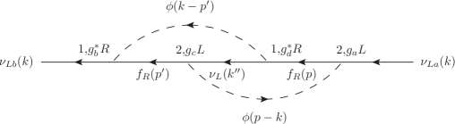
Figure 3: Equivalent form of diagram C in Fig. 2, with a relabeling of the internal momentum variables. Here we have defined $k^{\prime\prime}=p+p^{\prime}-k$.

Invoking once again the two-body kinematics argument, we see that in Eq. (4.47) the contribution from the thermal part of the diagonal $f$ propagators is suppressed, as well as the contribution from the thermal part of the diagonal $\phi$ propagators in Eq. (4.49). Thus, approximating the vacuum part of the diagonal propagators by their high $k$ limit,

$$-i\left(\Sigma^{(CI)}_{12}(k)\right)_{ba} = \sum_{c,d}\int\frac{d^{4}p}{(2\pi)^{4}}\frac{d^{4}p^{\prime}}{(2\pi)^{4}}i\Delta^{(\phi)}_{21}(p)i\Delta^{(\phi)}_{12}(p^{\prime})(i\eta_{1}g^{\ast}_{b}R)iS^{(f)}_{0}(-p^{\prime},k)(i\eta_{1}g_{c}L)$$ (4.50)

$$\mbox{}\times\left(iS^{(\nu)}_{12}(k^{\prime})\right)_{cd}(i\eta_{2}g^{\ast}_{d}R)\left(-iS^{(f)}_{0}(p,k)\right)(i\eta_{2}g_{a}L)\,,$$

$$-i\left(\Sigma^{(CII)}_{12}(k)\right)_{ba} = \sum_{c,d}\int\frac{d^{4}p}{(2\pi)^{4}}\frac{d^{4}p^{\prime}}{(2\pi)^{4}}\left(-i\Delta^{(\phi)}_{0}(p,-k)\right)i\Delta^{(\phi)}_{0}(p^{\prime},-k)(i\eta_{1}g^{\ast}_{b}R)iS^{(f)}_{12}(p^{\prime})(i\eta_{2}g_{c}L)$$ (4.51)

$$\mbox{}\times\left(iS^{(\nu)}_{21}(k^{\prime\prime})\right)_{cd}(i\eta_{1}g^{\ast}_{d}R)iS^{(f)}_{12}(p)(i\eta_{2}g_{a}L)\,.$$

4.4 Summary

In summary, we are left with four contributions,

$$\left(\Sigma_{12}\right)_{ba}=\left(\Sigma^{(A)}_{12}\right)_{ba}+\left(\Sigma^{(B)}_{12}\right)_{ba}+\left(\Sigma^{(CI)}_{12}\right)_{ba}+\left(\Sigma^{(CII)}_{12}\right)_{ba}\,,$$ (4.52)

given by Eqs. (4.26), (4.2), (4.50) and (4.51). In those formulas, $\Delta^{(\phi)}_{0}$ and $S^{(f)}_{0}$ are the free fermion and scalar propagators, respectively, in the high energy limit, defined in Eqs. (4.24) and (4.42). From the expressions in those equations it follows that only B and CI contribute in a pure $\phi$ background (no $f$ in the background) while in a pure $f$ background (no $\phi$ in the background) only A and CII contribute. In either case, the diagrams CI and CII exist only if $\phi$ is a real scalar. For a complex $\phi$ only diagrams A and B exist. In the next section we consider precisely the former case, namely a pure $\phi$ background. We determine the damping terms according to the scheme explained in Section 2, and evaluate explicitly the integrals involved for some illustrative background conditions.

Before moving ahead, it is worth to emphasize the following. Only diagrams A and B suffer from the pinch singularities. Eqs. (4.26) and (4.2) give us convenient starting points to compute the contribution from diagrams A and B, respectively, within the high-momentum approximation that we restrict ourselves here. However, the pinch singularities are already tamed in Eqs. (4.20) and (4.40), respectively, and those expressions can be used to compute the corresponding contributions in other situations of interest.

5 A pure $\phi$ background

For definiteness, in the remainder of this work we consider only a $\phi$ background with no fermions $f$. We will calculate $\Sigma_{i}$ for this case next. From the result we will determine the damping matrix in Section 5.2.

5.1 Expression for $\Sigma_{i}$

The starting point is the expression for each of the diagrams B and CI we have obtained in Eqs. (4.2) and (4.50), explicitly

$$-i\left(\Sigma^{(B)}_{12}(k)\right)_{ba} = (2K_{ba})\int\frac{d^{4}p}{(2\pi)^{4}}\frac{d^{4}p^{\prime}}{(2\pi)^{4}}i\Delta^{(\phi)}_{21}(p)i\Delta^{(\phi)}_{12}(p^{\prime})$$

$$\mbox{}\times RiS^{(f)}_{0}(p,k)LiS^{(\nu)}_{12}(k^{\prime})R\left(-iS^{(f)}_{0}(p,k)\right)L\,,$$

$$-i\left(\Sigma^{(CI)}_{12}(k)\right)_{ba} = (2K_{ba})\int\frac{d^{4}p}{(2\pi)^{4}}\frac{d^{4}p^{\prime}}{(2\pi)^{4}}i\Delta^{(\phi)}_{21}(p)i\Delta^{(\phi)}_{12}(p^{\prime})$$ (5.1)

$$\mbox{}\times RiS^{(f)}_{0}(-p^{\prime},k)LiS^{(\nu)}_{12}(k^{\prime})R\left(-iS^{(f)}_{0}(p,k)\right)L\,,$$

where

$$K_{ba}=\frac{1}{2}g^{\ast}_{b}g_{a}\left(\sum_{c}|g_{c}|^{2}\right)\,.$$ (5.2)

We have used the fact that the neutrino propagator is diagonal in flavor space, and we are defining $K_{ba}$ with the factor of $1/2$ for later convenience when we identify $\Sigma_{i}$. It it understood that for a complex $\phi$ only $\Sigma^{(B)}_{12}$ contributes, while if $\phi$ is real then $\Sigma^{(CI)}_{12}$ also contributes but in that case the chemical potential $\alpha_{\phi}=0$ in the final evaluation of the integrals involving the distribution functions.

We write the formulas for the propagators as follows. For the fermion $f$, remembering Eq. (4.42), we have

$$RS^{(f)}_{0}(p,k)L=S_{f}(p,k)L\,,$$ (5.3)

with

$$S_{f}(p,k)\equiv\frac{p\hbox to0.0pt{\hss/}+k\hbox to0.0pt{\hss/}}{2p\cdot k}\,.$$ (5.4)

For the neutrino and the scalar propagators,

$$S^{(\nu)}_{12}(k^{\prime}) = 2\pi i\delta(k^{\prime\,2})n_{F}(x^{\prime}_{\nu})\epsilon(k^{\prime}\cdot u)Ls_{\nu}(k^{\prime})\,,$$

$$\Delta^{(\phi)}_{21}(p) = -2\pi i\delta(p^{2}-m^{2}_{\phi})e^{x_{\phi}}n_{B}(x_{\phi})\epsilon(p\cdot u)\,,$$

$$\Delta^{(\phi)}_{12}(p^{\prime}) = -2\pi i\delta(p^{\prime\,2}-m^{2}_{\phi})n_{B}(x^{\prime}_{\phi})\epsilon(p^{\prime}\cdot u)\,,$$ (5.5)

where

$$s_{\nu}(k^{\prime})=k\hbox to0.0pt{\hss/}^{\prime}\,,$$ (5.6)

$\epsilon(z)=\theta(z)-\theta(-z)$ with $\theta(z)$ being the unit step function, the fermion and boson distribution functions $n_{F,B}$ are defined in Eqs. (2.9) and (3.4), and

$$x^{\prime}_{\nu} = \beta k^{\prime}\cdot u-\alpha_{\nu}\,,$$

$$x_{\phi} = \beta p\cdot u-\alpha_{\phi}\,,$$

$$x^{\prime}_{\phi} = \beta p^{\prime}\cdot u-\alpha_{\phi}\,.$$ (5.7)

It is useful to remember that the relation $k^{\prime}=k+p-p^{\prime}$ (actually the definition of $k^{\prime}$), implies the following relation

$$x_{\nu}+x_{\phi}=x^{\prime}_{\nu}+x^{\prime}_{\phi}\,.$$ (5.8)

Substituting Eq. (5.1) in Eq. (5.1), we then have

$$-i\left(\Sigma^{(B)}_{12}(k)\right)_{ba} = -(2K_{ba})\int\frac{d^{4}p}{(2\pi)^{3}}\frac{d^{4}p^{\prime}}{(2\pi)^{3}}\frac{d^{4}k^{\prime}}{(2\pi)^{3}}(2\pi)^{4}\delta^{(4)}(k^{\prime}+p^{\prime}-k-p)$$

$$\mbox{}\times{}\delta(p^{2}-m^{2}_{\phi})\delta(p^{\prime\,2}-m^{2}_{\phi})\delta(k^{\prime\,2})\epsilon(p\cdot u)\epsilon(p^{\prime}\cdot u)\epsilon(k^{\prime}\cdot u)$$

$$\mbox{}\times\left[S_{f}(p,k)s_{\nu}(k^{\prime})S_{f}(p,k)L\right]E^{\prime}\,,$$

$$-i\left(\Sigma^{(CI)}_{12}(k)\right)_{ba} = -(2K_{ba})\int\frac{d^{4}p}{(2\pi)^{3}}\frac{d^{4}p^{\prime}}{(2\pi)^{3}}\frac{d^{4}k^{\prime}}{(2\pi)^{3}}(2\pi)^{4}\delta^{(4)}(k^{\prime}+p^{\prime}-k-p)$$ (5.9)

$$\mbox{}\times\delta(p^{2}-m^{2}_{\phi})\delta(p^{\prime\,2}-m^{2}_{\phi})\delta(k^{\prime\,2})\epsilon(p\cdot u)\epsilon(p^{\prime}\cdot u)\epsilon(k^{\prime}\cdot u)$$

$$\mbox{}\times\left[S_{f}(-p^{\prime},k)s_{\nu}(k^{\prime})S_{f}(p,k)L\right]E^{\prime}\,,$$

where

$$E^{\prime}\equiv e^{x_{\phi}}n_{B}(x_{\phi})n_{B}(x^{\prime}_{\phi})n_{F}(x^{\prime}_{\nu})\,.$$ (5.10)

In writing Eq. (5.1) we have taken $k^{\prime}$ to be an arbitrary variable but inserted a factor of $\delta^{(4)}(k+p-k^{\prime}-p^{\prime})$ and integrate over $k^{\prime}$.

Letting $X=B,CI$, the corresponding contributions to the absorptive part of the self-energy, identified by

$$\left(\Sigma_{i}\right)_{ba}=\frac{\Sigma_{12}}{2in_{F}(x_{\nu})}\,,$$ (5.11)

are then given by

$$\left(\Sigma^{(X)}_{i}(k)\right)_{ba} = -K_{ba}\int\frac{d^{4}p}{(2\pi)^{3}}\frac{d^{4}p^{\prime}}{(2\pi)^{3}}\frac{d^{4}k^{\prime}}{(2\pi)^{3}}(2\pi)^{4}\delta^{(4)}(k+p-k^{\prime}-p^{\prime})$$ (5.12)

$$\mbox{}\times\delta(p^{2}-m^{2}_{\phi})\delta(p^{\prime\,2}-m^{2}_{\phi})\delta(k^{\prime\,2})\epsilon(p\cdot u)\epsilon(p^{\prime}\cdot u)\epsilon(k^{\prime}\cdot u)M^{(X)}_{\nu}E\,,$$

where we have used the identity

$$\frac{1}{n_{F}(x_{\nu})}E^{\prime}\equiv E=n_{B}(x_{\phi})\left(1+n_{B}(x^{\prime}_{\phi})\right)-n_{F}(x^{\prime}_{\nu})\left(n_{B}(x_{\phi})-n_{B}(x^{\prime}_{\phi})\right)\,,$$ (5.13)

and we have defined

$$M^{(B)}_{\nu} = S_{f}(p,k)s_{\nu}(k^{\prime})S_{f}(p,k)L\,,$$

$$M^{(CI)}_{\nu} = S_{f}(-p^{\prime},k)s_{\nu}(k^{\prime})S_{f}(p,k)L\,.$$ (5.14)

Next we carry out the integrals over $p^{0},p^{\prime\,0},k^{\prime\,0}$. Starting with $k^{\prime\,0}$,

$$\left(\Sigma^{(X)}_{i}(k)\right)_{ba} = -K_{ba}\int\frac{d^{4}p}{(2\pi)^{3}}\frac{d^{4}p^{\prime}}{(2\pi)^{3}}\frac{d^{3}\kappa^{\prime}}{(2\pi)^{3}2\omega_{\kappa^{\prime}}}\delta(p^{2}-m^{2}_{\phi})\delta(p^{\prime\,2}-m^{2}_{\phi})\epsilon(p\cdot u)\epsilon(p^{\prime}\cdot u)$$ (5.15)

$$\mbox{}\times(2\pi)^{4}\left\{\delta^{(4)}(k+p-k^{\prime}-p^{\prime})M^{(X)}_{\nu}E_{\nu}-\delta^{(4)}(k+p+k^{\prime}-p^{\prime})M^{(X)}_{\bar{\nu}}E_{\bar{\nu}}\right\}\,,$$

where

$$E_{\nu} = n_{B}(x_{\phi})\left(1+n_{B}(x^{\prime}_{\phi})\right)-f_{\nu}(\omega_{\kappa^{\prime}})\left(n_{B}(x_{\phi})-n_{B}(x^{\prime}_{\phi})\right)$$

$$E_{\bar{\nu}} = n_{B}(x^{\prime}_{\phi})\left(1+n_{B}(x_{\phi})\right)+f_{\bar{\nu}}(\omega_{\kappa^{\prime}})\left(n_{B}(x_{\phi})-n_{B}(x^{\prime}_{\phi})\right)\,,$$ (5.16)

and

$$M^{(X)}_{\bar{\nu}}=\left.M^{(X)}_{\nu}\right|_{k^{\prime}\rightarrow-k^{\prime}}\,,$$ (5.17)

understanding that from now on

$$k^{\prime}=(\omega_{\kappa^{\prime}},\vec{\kappa}^{\prime})\,,$$ (5.18)

with $\omega_{\kappa^{\prime}}=|\vec{\kappa}^{\prime}|\equiv\kappa^{\prime}$. To arrive at Eq. (5.15) we have also made the change of variable $\vec{\kappa}^{\prime}\rightarrow-\vec{\kappa}^{\prime}$ in the second term. Proceeding in a similar way with the integrals over $p^{0}$ and $p^{\prime\,0}$,

$$\left(\Sigma^{(X)}_{i}(k)\right)_{ba} = -K_{ba}\int\frac{d^{3}p}{(2\pi)^{3}2E_{p}}\frac{d^{3}p^{\prime}}{(2\pi)^{3}2E_{p^{\prime}}}\frac{d^{3}\kappa^{\prime}}{(2\pi)^{3}2\omega_{\kappa^{\prime}}}$$ (5.19)

$$\mbox{}\times\sum_{\lambda,\lambda^{\prime}}(2\pi)^{4}\left\{\delta^{(4)}(k+\lambda p-k^{\prime}-\lambda^{\prime}p^{\prime})M^{(X)}_{\nu,\lambda\lambda^{\prime}}E_{\nu,\lambda\lambda^{\prime}}\right.$$

$$\mbox{}-\left.\delta^{(4)}(k+\lambda p+k^{\prime}-\lambda^{\prime}p^{\prime})M^{(X)}_{\bar{\nu},\lambda\lambda^{\prime}}E_{\bar{\nu},\lambda\lambda^{\prime}}\right\}\,,$$

where

$$M^{(B)}_{\nu,\lambda\lambda^{\prime}} = S_{f}(\lambda p,k)s_{\nu}(k^{\prime})S_{f}(\lambda p,k)L\,,$$

$$M^{(CI)}_{\nu,\lambda\lambda^{\prime}} = S_{f}(-\lambda^{\prime}p^{\prime},k)s_{\nu}(k^{\prime})S_{f}(\lambda p,k)L\,,$$

$$M^{(X)}_{\bar{\nu},\lambda\lambda^{\prime}} = \left.M^{(X)}_{\nu,\lambda\lambda^{\prime}}\right|_{k^{\prime}\rightarrow-k^{\prime}}\,.$$ (5.20)

We have defined

$$E_{\nu,\lambda\lambda^{\prime}}=\left.E_{\nu}\right|_{p\rightarrow\lambda p,\,p^{\prime}\rightarrow\lambda^{\prime}p^{\prime}}$$ (5.21)

and similarly for $E_{\bar{\nu},\lambda\lambda^{\prime}}$, and from now on $p$ and $p^{\prime}$ are on-shell. The formulas are given explicitly in Table 1.

$E_{\nu,++}=f(1+f^{\prime})-f^{\prime}_{\nu}(f-f^{\prime})$	$\nu_{a,b}(k)+\phi(p)\leftrightarrow\nu_{i}(k^{\prime})+\phi(p^{\prime})$
$E_{\nu,-+}=-(1+\bar{f})(1+f^{\prime})+f^{\prime}_{\nu}(1+\bar{f}+f^{\prime})$	$\nu_{a,b}(k)\leftrightarrow\nu_{i}(k^{\prime})+\bar{\phi}(p)+\phi(p^{\prime})$
$E_{\nu,+-}=-f\bar{f}^{\prime}-f^{\prime}_{\nu}(1+f+\bar{f}^{\prime})$	$\nu_{a,b}(k)+\phi(p)+\bar{\phi}(p^{\prime})\leftrightarrow\nu_{i}(k^{\prime})$
$E_{\nu,--}=(1+\bar{f})\bar{f}^{\prime}+f^{\prime}_{\nu}(\bar{f}-\bar{f}^{\prime})$	$\nu_{a,b}(k)+\bar{\phi}(p^{\prime})\leftrightarrow\nu_{i}(k^{\prime})+\bar{\phi}(p)$
$E_{\bar{\nu},++}=(1+f)f^{\prime}+\bar{f}^{\prime}_{\nu}(f-f^{\prime})$	$\nu_{a,b}(k)+\bar{\nu}_{i}(\bar{k}^{\prime})+\phi(p)\leftrightarrow\phi(p^{\prime})$
$E_{\bar{\nu},-+}=-\bar{f}f^{\prime}-\bar{f}^{\prime}_{\nu}(1+\bar{f}+f^{\prime})$	$\nu_{a,b}(k)+\bar{\nu}_{i}(\bar{k}^{\prime})\leftrightarrow\bar{\phi}(p)+\phi(p^{\prime})$
$E_{\bar{\nu},+-}=-(1+f)(1+\bar{f}^{\prime})+\bar{f}^{\prime}_{\nu}(1+f+\bar{f}^{\prime})$	$\nu_{a,b}(k)+\bar{\nu}_{i}(\bar{k}^{\prime})+\phi(p)+\bar{\phi}(p^{\prime})\leftrightarrow 0$
$E_{\bar{\nu},--}=\bar{f}(1+\bar{f}^{\prime})-\bar{f}^{\prime}_{\nu}(\bar{f}-\bar{f}^{\prime})$	$\nu_{a,b}(k)+\bar{\nu}_{i}(\bar{k}^{\prime})+\bar{\phi}(p^{\prime})\leftrightarrow\bar{\phi}(p)$

Table 1: Correspondence between the $E_{\nu,\lambda\lambda^{\prime}}$ and $E_{\bar{\nu},\lambda\lambda^{\prime}}$ factors defined in Eq. (5.21), and the process that contributes to the $\nu(k)$ damping via Eq. (5.19). To simplify the notation we are using the shorthands shown in Eq. (5.1) for the various distribution functions.

To simplify the notation in the formulas summarized in Table 1 we have introduce the shorthands

$$f=f_{\phi}(E_{p}),\quad f^{\prime}=f_{\phi}(E_{p^{\prime}}),\quad f^{\prime}_{\nu}={f_{\nu}(\omega_{\kappa^{\prime}})}$$

$$\bar{f}=f_{\bar{\phi}}(E_{p}),\quad\bar{f}^{\prime}=f_{\bar{\phi}}(E_{p^{\prime}}),\quad\bar{f}^{\prime}_{\nu}=f_{\bar{\nu}}(\omega_{\kappa^{\prime}})\,.$$ (5.22)

The formulas for $E_{\bar{\nu},\lambda\lambda^{\prime}}$ are obtained from those for $E_{\nu,\lambda\lambda^{\prime}}$ by making the replacement $f^{\prime}_{\nu}\rightarrow(1-\bar{f}^{\prime}_{\nu})$. Each of the terms in Eq. (5.19) represents a contribution to $\Sigma_{i}$ from a specific physical process, as indicated in Table 1.

5.2 Damping matrix

We write Eq. (5.1) in the form

$$M^{(X)}_{\nu}=\frac{N^{(X)}L}{D^{(X)}}\,,\\$$

where

$$D^{(B)} = (2p\cdot k)^{2}\,,$$

$$D^{(CI)} = (-2p^{\prime}\cdot k)(2p\cdot k)\,,$$ (5.23)

and

$$N^{(B)} = (k\hbox to0.0pt{\hss/}+p\hbox to0.0pt{\hss/})k\hbox to0.0pt{\hss/}^{\prime}(k\hbox to0.0pt{\hss/}+p\hbox to0.0pt{\hss/})\,,$$

$$N^{(CI)} = (k\hbox to0.0pt{\hss/}-p\hbox to0.0pt{\hss/}^{\prime})k\hbox to0.0pt{\hss/}^{\prime}(k\hbox to0.0pt{\hss/}+p\hbox to0.0pt{\hss/})\,.$$ (5.24)

The expressions for the $N^{(X)}$ are reduced by using the identity

$$\gamma_{\lambda}\gamma_{\mu}\gamma_{\nu}=C_{\lambda\mu\nu\rho}\gamma^{\rho}+i\epsilon_{\lambda\mu\nu\rho}\gamma^{\rho}\gamma^{5}\,,$$ (5.25)

where

$$C_{\lambda\mu\nu\rho}=g_{\lambda\mu}g_{\nu\rho}-g_{\lambda\nu}g_{\mu\rho}+g_{\lambda\rho}g_{\mu\nu}\,.$$ (5.26)

After the integrations over $k^{\prime},p,p^{\prime}$ the only vectors remaining are $k$ and $u$, and then the terms with the antisymmetric tensor vanish. Thus we can replace in the integrand

$$N^{(X)}\rightarrow\ell^{(X)\rho}\gamma_{\rho}\,,$$ (5.27)

where

$$\ell^{(X)}_{\rho} = C_{\lambda\mu\nu\rho}(k+p)^{\lambda}k^{\prime\,\mu}(k+p)^{\nu}\,,$$

$$\ell^{(X)}_{\rho} = C_{\lambda\mu\nu\rho}(k-p^{\prime})^{\lambda}k^{\prime\,\mu}(k+p)^{\nu}\,.$$ (5.28)

Then, corresponding to each diagram $X=B,CI$ we have

$$\left(V^{(X)\mu}_{i}(\omega,\vec{\kappa})\right)_{ba} = -K_{ba}\int\frac{d^{3}p}{(2\pi)^{3}2E_{p}}\frac{d^{3}p^{\prime}}{(2\pi)^{3}2E_{p^{\prime}}}\frac{d^{3}\kappa^{\prime}}{(2\pi)^{3}2\omega_{\kappa^{\prime}}}$$ (5.29)

$$\mbox{}\times\sum_{\lambda,\lambda^{\prime}}\left(\frac{\ell^{(X)\mu}_{\lambda\lambda^{\prime}}}{D^{(X)}_{\lambda\lambda^{\prime}}}\right)(2\pi)^{4}\left\{\delta^{(4)}(k+\lambda p-k^{\prime}-\lambda^{\prime}p^{\prime})E_{\nu,\lambda\lambda^{\prime}}\right.$$

$$\mbox{}+\left.\delta^{(4)}(k+\lambda p+k^{\prime}-\lambda^{\prime}p^{\prime})E_{\bar{\nu}\lambda\lambda^{\prime}}\right\}\,,$$

where

$$\ell^{(X)\mu}_{\lambda\lambda^{\prime}} \equiv \left.\ell^{(X)\mu}\right|_{p\rightarrow\lambda p,p^{\prime}\rightarrow\lambda^{\prime}p^{\prime}},$$

$$D^{(X)}_{\lambda\lambda^{\prime}} \equiv \left.D^{(X)}\right|_{p\rightarrow\lambda p,p^{\prime}\rightarrow\lambda^{\prime}p^{\prime}}\,.$$ (5.30)

Since the formulas for $\Gamma$ are given in terms of $n\cdot V_{i}(\kappa,\vec{\kappa})$ (for neutrinos), or $n\cdot V_{i}(-\kappa,-\vec{\kappa})$ (for antineutrinos), we consider the evaluation of $\Sigma_{i}$ for $k^{\mu}=\omega n^{\mu}$ (which in particular implies $k^{2}=0$), and in the end put $\omega=\pm\kappa$ (for neutrinos or antineutrinos, respectively). From now on we thus set $k^{2}=0$.

We evaluate $n\cdot\ell$ and $n\cdot\ell^{\prime}$, putting $k^{\mu}=\omega n^{\mu}$ as we already stated. Then doing the algebra, remembering to set $n^{2}=0$,

$$n\cdot\ell^{(B)} = 2(n\cdot p)(k^{\prime}\cdot p)\,,$$

$$n\cdot\ell^{(CI)} = -(n\cdot p)(k^{\prime}\cdot p^{\prime})-(n\cdot p^{\prime})(k^{\prime}\cdot p)\,,$$ (5.31)

and therefore

$$\frac{n\cdot\ell^{(B)}}{D^{(B)}} = \frac{1}{2\omega}\frac{k^{\prime}\cdot p}{k\cdot p}\,,$$

$$\frac{n\cdot\ell^{(CI)}}{D^{(CI)}} = \frac{1}{4\omega}\frac{k^{\prime}\cdot p^{\prime}}{k\cdot p^{\prime}}+\frac{1}{4\omega}\frac{k^{\prime}\cdot p}{k\cdot p}\,.$$ (5.32)

Up to this moment we have only used straightforward algebra to arrive here from Eq. (5.2). We now invoke the high energy limit we are considering. The momentum delta functions set $k^{\prime}=k+p-p^{\prime}$. Therefore, to leading order in $k$, we put $k^{\prime}\rightarrow k$ in the above and for either diagram we have

$$\frac{n\cdot\ell^{(X)}}{D^{(X)}}=\frac{1}{2\omega}\,.$$ (5.33)

For the antineutrino part, the delta function gives $k^{\prime}=-k-p+p^{\prime}$, therefore the replacement is $k^{\prime}\rightarrow-k$. Putting all this together we then have, from Eq. (5.29),

$$\left(n\cdot V^{(X)}_{i}(\omega,\omega\hat{\kappa})\right)_{ba} = -\frac{K_{ba}}{2\omega}\int\frac{d^{3}p}{(2\pi)^{3}2E_{p}}\frac{d^{3}p^{\prime}}{(2\pi)^{3}2E_{p^{\prime}}}\frac{d^{3}\kappa^{\prime}}{(2\pi)^{3}2\omega_{\kappa^{\prime}}}$$ (5.34)

$$\mbox{}\times\sum_{\lambda,\lambda^{\prime}}(2\pi)^{4}\left\{\delta^{(4)}(k+\lambda p-k^{\prime}-\lambda^{\prime}p^{\prime})E_{\nu,\lambda\lambda^{\prime}}\right.$$

$$\mbox{}-\left.\delta^{(4)}(k+\lambda p+k^{\prime}-\lambda^{\prime}p^{\prime})E_{\bar{\nu}\lambda\lambda^{\prime}}\right\}\,.$$

The damping matrix is given by

$$-\frac{1}{2}\Gamma^{(2)}=\left\{\begin{array}[]{ll}n\cdot V^{(B)}_{i}(\kappa,\vec{\kappa})&(\nu)\\ n\cdot V^{(B)\ast}_{i}(-\kappa,-\vec{\kappa})&(\bar{\nu})\,,\end{array}\right.$$ (5.35)

or

$$-\frac{1}{2}\Gamma^{(2)}=\left\{\begin{array}[]{ll}n\cdot V^{(B)}_{i}(\kappa,\vec{\kappa})+n\cdot V^{(CI)}_{i}(\kappa,\vec{\kappa})&(\nu)\\ n\cdot V^{(B)\ast}_{i}(-\kappa,-\vec{\kappa})+n\cdot V^{(CI)\ast}_{i}(-\kappa,-\vec{\kappa})&(\bar{\nu})\,,\end{array}\right.$$ (5.36)

for a complex or real $\phi$, respectively. The final expressions for both diagram contributions $n\cdot V^{(X)}_{i}$, given in Eq. (5.34), are formally the same. But it must be understood that for a real $\phi$ the distribution functions of the $\phi$ have $\alpha_{\phi}=0$, or equivalently $f_{\bar{\phi}}=f_{\phi}$.

Not all the terms in Eq. (5.34) contribute, depending on whether $\omega$ is positive or negative. Equivalently, the corresponding processes are inhibited by the kinematics. In addition we will assume that there are no neutrinos in the background. The result is that for the neutrinos ($\omega$ positive) only the terms $E_{\nu,++},E_{\nu,--}$ contribute, while for the antineutrinos ($\omega$ negative) only $E_{\bar{\nu},++},E_{\bar{\nu},--}$ contribute.

Denoting by $\Gamma^{(\nu)}$ and $\Gamma^{(\bar{\nu})}$ the matrices for neutrinos and antineutrinos, respectively, for the case of a complex $\phi$ we then have from Eq. (5.34),

$$\frac{1}{2}\Gamma^{(\nu)}_{ba} = \frac{K_{ba}\gamma^{(\nu)}}{2\kappa}\,,$$

$$\frac{1}{2}\Gamma^{(\bar{\nu})}_{ba} = \frac{K^{\ast}_{ba}\gamma^{(\bar{\nu})}}{2\kappa}\,,$$ (5.37)

where

$$\gamma^{(\nu)} = \int\frac{d^{3}p}{(2\pi)^{3}2E_{p}}\frac{d^{3}p^{\prime}}{(2\pi)^{3}2E_{p^{\prime}}}\frac{d^{3}\kappa^{\prime}}{(2\pi)^{3}2\omega_{\kappa^{\prime}}}$$

$$\mbox{}(2\pi)^{4}\left\{\delta^{(4)}(k+p-k^{\prime}-p^{\prime})E_{\nu,++}+\delta^{(4)}(k+p^{\prime}-k^{\prime}-p)E_{\nu,--}\right\}\,,$$

$$\gamma^{(\bar{\nu})} = \int\frac{d^{3}p}{(2\pi)^{3}2E_{p}}\frac{d^{3}p^{\prime}}{(2\pi)^{3}2E_{p^{\prime}}}\frac{d^{3}\kappa^{\prime}}{(2\pi)^{3}2\omega_{\kappa^{\prime}}}$$ (5.38)

$$\mbox{}(2\pi)^{4}\left\{\delta^{(4)}(k+p^{\prime}-k^{\prime}-p)E_{\bar{\nu},++}+\delta^{(4)}(k+p-k^{\prime}-p^{\prime})E_{\bar{\nu},--}\right\}\,,$$

with

$$E_{\nu++} = f_{\phi}(E_{p})(1+f_{\phi}(E_{p^{\prime}}))\,,$$

$$E_{\nu--} = f_{\bar{\phi}}(E_{p^{\prime}})(1+f_{\bar{\phi}}(E_{p}))\,,$$

$$E_{\bar{\nu}++} = f_{\phi}(E_{p^{\prime}})(1+f_{\phi}(E_{p}))\,,$$

$$E_{\bar{\nu}--} = f_{\bar{\phi}}(E_{p})(1+f_{\bar{\phi}}(E_{p^{\prime}}))\,.$$ (5.39)

Relabeling the $p,p^{\prime}$ integration variables in some terms, we can see that $\gamma^{(\bar{\nu})}=\gamma^{(\nu)}$. Therefore, in explicit form, Eq. (5.2) becomes

$$\frac{1}{2}\Gamma^{(\nu)}_{ba} = \frac{K_{ba}\gamma^{(\phi)}}{2\kappa}\,,$$

$$\frac{1}{2}\Gamma^{(\bar{\nu})}_{ba} = \frac{K^{\ast}_{ba}\gamma^{(\phi)}}{2\kappa}\,,$$ (5.40)

where

$$\gamma_{\phi} \equiv \int\frac{d^{3}p}{(2\pi)^{3}2E_{p}}\frac{d^{3}p^{\prime}}{(2\pi)^{3}2E_{p^{\prime}}}\frac{d^{3}\kappa^{\prime}}{(2\pi)^{3}2\omega_{\kappa^{\prime}}}$$ (5.41)

$$\mbox{}(2\pi)^{4}\delta^{(4)}(k+p-k^{\prime}-p^{\prime})\left\{f_{\phi}(E_{p})(1+f_{\phi}(E_{p^{\prime}}))+f_{\bar{\phi}}(E_{p})(1+f_{\bar{\phi}}(E_{p^{\prime}}))\right\}\,.$$

As already stated, Eq. (5.2) holds for a complex $\phi$. For a real $\phi$ the formula is the same but with the replacement $2\kappa\rightarrow\kappa$, and putting $f_{\bar{\phi}}=f_{\phi}$ in Eq. (5.41).

5.3 Example evaluation of integrals

In the dilute gas approximation (i.e., neglecting the terms with the product of the distribution function),

$$\gamma_{\phi}=\int\frac{d^{3}p}{(2\pi)^{3}2E_{p}}(f_{\phi}(E_{p})+f_{\bar{\phi}}(E_{p}))J\,,$$ (5.42)

where

$$J=\int\frac{d^{3}p^{\prime}}{(2\pi)^{3}2E_{p^{\prime}}}\frac{d^{3}\kappa^{\prime}}{(2\pi)^{3}2\omega_{\kappa^{\prime}}}(2\pi)^{4}\delta^{(4)}(k+p-k^{\prime}-p^{\prime})\,.$$ (5.43)

It is straightforward to evaluate the $J$ integral. Let us define

$$q=k+p\,,$$ (5.44)

and

$$s=q^{2}\,.$$ (5.45)

We then obtain

$$J=\frac{1}{4\pi}\left(\frac{p^{\prime\,\ast}}{\sqrt{s}}\right)\theta(\sqrt{s}-E^{\ast}_{p^{\prime}})\theta(E^{\ast}_{p^{\prime}}-m_{\phi})\,,$$ (5.46)

where

$$E^{\ast}_{p^{\prime}}=\frac{s+m^{2}_{\phi}}{2\sqrt{s}}\,,$$ (5.47)

and

$$p^{\prime\,\ast}=\sqrt{E^{\ast\,2}_{p^{\prime}}-m^{2}_{\phi}}=\frac{s-m^{2}_{\phi}}{2\sqrt{s}}\,.$$ (5.48)

From the definition in Eq. (5.45),

$$s = m^{2}_{\phi}+2k\cdot p$$ (5.49)

$$= m^{2}_{\phi}+2\kappa E_{p}(1-v_{p}\cos\theta_{p})\,,$$

where

$$\cos\theta_{p}=\hat{\kappa}\cdot\hat{p}\,,$$ (5.50)

and

$$v_{p}=\frac{|\vec{p}|}{E_{p}}\,.$$ (5.51)

Thus for any value of $\vec{p}$, we have $s>m^{2}_{\phi}$, and this implies that the two step functions in Eq. (5.46) are automatically satisfied. Therefore, we can take $J$ to be simply

$$J=\frac{1}{8\pi}\left(\frac{s-m^{2}_{\phi}}{s}\right)=\frac{1}{8\pi}\left(1-\frac{m^{2}_{\phi}}{s}\right)=\frac{1}{8\pi}\left(1-\frac{m^{2}_{\phi}}{m^{2}_{\phi}+\kappa E_{p}(1-v_{p}\cos\theta_{p})}\right)$$ (5.52)

In principle we can use this to do the remaining integral over $\vec{p}$ to evaluate $\gamma_{\phi}$ for different background distribution functions. However, since we are interested in the high $\kappa$ limit, we retain just the leading term

$$J=\frac{1}{8\pi}\,,$$ (5.53)

which in turn gives

$$\gamma_{\phi}=\frac{1}{8\pi}J_{\phi}\,.$$ (5.54)

Thus from Eq. (5.2), for a complex $\phi$,

$$\frac{1}{2}\Gamma^{(\nu)}_{ba}=\frac{K_{ba}J_{\phi}}{16\pi\kappa}\,,$$ (5.55)

where $J_{\phi}$ is defined in Eq. (3.25). For a real $\phi$

$$\frac{1}{2}\Gamma^{(\nu)}_{ba}=\frac{K_{ba}J_{\phi}}{8\pi\kappa}\,,$$ (5.56)

and $J_{\phi}$ is evaluated putting $f_{\bar{\phi}}=f_{\phi}$. In either case the formula for $\Gamma^{(\nu)}_{ba}$ is obtained by replacing $K_{ba}\rightarrow K^{\ast}_{ba}$. Thus, for example, using Eq. (3.26), Eq. (5.55) yields

$$\frac{1}{2}\Gamma^{(\nu)}_{ba}=K_{ba}\left\{\begin{array}[]{ll}\frac{n_{\phi}+n_{\bar{\phi}}}{32\pi\kappa m_{\phi}}&\mbox{(NR)}\\[12.0pt] \frac{T^{2}}{192\pi\kappa}&\mbox{(UR)}\,.\end{array}\right.$$ (5.57)

These are valid for a complex $\phi$. For a real $\phi$, the corresponding formulas are

$$\frac{1}{2}\Gamma^{(\nu)}_{ba}=K_{ba}\left\{\begin{array}[]{ll}\frac{n_{\phi}}{8\pi\kappa m_{\phi}}&\mbox{(NR)}\\[12.0pt] \frac{T^{2}}{96\pi\kappa}&\mbox{(UR)}\,.\end{array}\right.$$ (5.58)

For the antineutrinos, the damping matrix is given by the same formulas, but replacing $K_{ba}\rightarrow K^{\ast}_{ba}$.

Comparing Eq. (5.55) (or Eq. (5.56)) with Eq. (3.24) we see that the ratio of the imaginary part (damping) to the real part of the effective potential is $\sim g^{2}/16\pi$. This contrasts with the result in the case of a normal matter background. In that case the same ratio is further suppressed by the mass factor $\kappa m_{e}/m^{2}_{W}$ (for $\kappa>m_{e}$) or $\kappa^{2}/m^{2}_{W}$ (for $m_{e}>\kappa$)[29]. Therefore, in situations where the effective potential due to a light scalar background may be relevant, the damping effects may be important since they are not suppressed by the mass factors. On the other hand, the relative importance of such damping effects may be negligible if all $g_{a}$ couplings are too small.

5.4 Discussion

We have obtained Eqs. (5.57) and (5.58), or their more general versions given in Eqs. (5.55) and (5.56), by purposely considering a background with only $\phi$ particles and no fermions $f$. However the inclusion of the fermion contribution can be carried out straightforwardly in analogous fashion. It involves calculating in a similar way the contributions denoted by $\Sigma^{(A)}_{12}$ and $\Sigma^{(CII)}_{12}$ in Eq. (4.52).

From a physical point of view, the damping matrix $\Gamma$ induces decoherence effects in the propagation of neutrinos. As emphasized in our previous work Ref. [16], and illustrated again here, the contribution to $\Gamma$ from the neutrino non-forward scattering process $\nu_{a}+x\rightarrow\nu_{b}+x$, where $x=f,\phi$, can be determined from the two-loop calculation of $\Sigma_{i}$. However, since in this case the initial neutrino state is depleted but the neutrino does not actually disappear (the initial neutrino transitions into a neutrino of a different flavor but does not decay into a $f\phi$ pair, for example), we have argued that the effects of the non-forward scattering processes are more appropriately interpreted in terms of decoherence phenomena rather than damping. Specifically, the damping matrix should be associated with decoherence effects in terms of the Lindblad equation and the notion of the stochastic evolution of the state vector[33, 34, 35, 36, 37]. The idea is to assume that the evolution due to the damping effects described by $\Gamma$ is accompanied by a stochastic evolution that cannot be described by the coherent evolution of the state vector. As discussed in detail in Ref. [16], the result of this idea is that the evolution of the system is described by the density matrix $\rho$ (in the sense that we can use it to calculate averages of quantum expectation values) that satisfies the Lindblad equation,

$$\partial_{t}\rho=-i[H_{r},\rho]+\sum_{n}\left\{L_{n}\rho L^{\dagger}_{n}-\frac{1}{2}L^{\dagger}_{n}L_{n}\rho-\frac{1}{2}\rho L^{\dagger}_{n}L_{n}\right\}\,,$$ (5.59)

where the $L_{n}$ matrices, representing the jump operators, are related to $\Gamma$ by

$$\Gamma=\sum_{n}L^{\dagger}_{n}L_{n}\,.$$ (5.60)

We refer to the terms involving the jump operators in the right-hand-side of Eq. (5.59) as the decoherence terms.

The damping matrix that we have determined from the two-loop self-energy calculation can be expressed in this form. For example, consider a real $\phi$ background. Eq. (5.56) can be written as

$$\Gamma^{(\ell)}_{ba}=(L^{(\ell)\dagger}_{\phi}L^{(\ell)}_{\phi})_{ba}=\sum_{c}(L^{(\ell)}_{\phi})^{\ast}_{cb}(L^{(\ell)}_{\phi})_{ca}\qquad(\ell=\nu,\bar{\nu})\,,$$ (5.61)

with

$$(L^{(\nu)}_{\phi})_{ca} = \sqrt{\frac{J_{\phi}}{8\pi\kappa}}\,g_{c}g_{a}\,,$$

$$(L^{(\bar{\nu})}_{\phi})_{ca} = (L^{(\nu)}_{\phi})^{\ast}_{ca}\,.$$ (5.62)

The $L$ matrices are expressed in terms of integrals over the background particles distribution functions. Going a step further, consider for illustrative purposes the NR limit. Then using Eq. (3.28),

$$(L^{(\nu)}_{\phi})_{ca} = \sqrt{\frac{n_{\phi}}{8\pi\kappa m_{\phi}}}\,g_{c}g_{a}\,,$$

$$(L^{(\bar{\nu})}_{\phi})_{ca} = \sqrt{\frac{n_{\phi}}{8\pi\kappa m_{\phi}}}\,g^{\ast}_{c}g^{\ast}_{a}\,.$$ (5.63)

It is straightforward to consider the addition of fermions $f$ in the background, or in fact more complicated superpositions of different background species. The evaluation of $\Sigma^{(A,CII)}_{12}$ would result in a matrix $L_{f}$ contributing in Eq. (5.60), so that

$$\Gamma^{(\ell)}=L^{(\ell)\dagger}_{\phi}L^{(\ell)}_{\phi}+L^{(\ell)\dagger}_{f}L^{(\ell)}_{f}\,.$$ (5.64)

The matrix $L^{(\ell)}_{f}$ would be given in terms of the fermion distribution by formulas analogous to Eq. (5.4). In general these formulas predict, for example, a specific dependence of the decoherence terms on the neutrino energy, depending on the background conditions. This complements the studies of the decoherence effects that are based on general considerations at a phenomenological level without a calculation of the decoherence terms. We do not pursue this any further here, but our results and calculations show the path for further applications along these lines.

6 Conclusions and outlook

In this work we have been concerned with the calculation of the damping terms that result from non-forward scattering processes when neutrinos propagate in a background of fermions ($f$) and scalars ($\phi$) interacting via a Yukawa-type interaction. We determine the contribution of those processes to the damping matrix $\Gamma$ from the two-loop calculation of the imaginary part of the thermal neutrino self-energy using the methods of thermal field theory (TFT). In the context of TFT the two-loop self-energy diagrams suffer from the so-called pinch singularities, which appear because the expressions contain two thermal propagators with the same momentum argument. A significant effort in this work was to show how those singularities are effectively handled by a judicious use of the properties and parametrizations of the thermal propagators. The final result of that exercise is a set of formulas for the two-loop contribution to the imaginary part of the self-energy from which the damping matrix is determined. The formulas are well-defined integrals over the background particle momentum distribution functions, which can be evaluated straightforwardly for different background conditions. For concreteness, we considered in detail a pure $\phi$ background, with no fermions $f$. We obtained the corresponding formulas for the damping terms, and evaluated them in some specific limits of the $\phi$ distribution functions.

As a guide to applications, we discussed briefly in Section 5.4 the connection between $\Gamma$ and the decoherence described in terms of the Lindblad equation. There we showed the explicit formulas obtained for the jump operators that appear in the Lindblad equation using the results of the calculation of $\Gamma$. We indicated how this approach can be extended to consider more general backgrounds that include the fermions $f$ or other particles.

The results we have presented extend our previous work and can be used to study the decoherence effects in a variety of physical contexts and environments. As a by-product, we have presented a detailed calculation of the imaginary part of the two-loop neutrino thermal self-energy, controlling the pinch singularities, using and illustrating a method that can be applied to perform similar calculations consistently in other situations of interest.

The work of S. S. is partially supported by DGAPA-UNAM (Mexico) Project No. IN103019.

References

- [1] G. Mangano, A. Melchiorri, P. Serra, A. Cooray and M. Kamionkowski, Cosmological bounds on dark matter-neutrino interactions, Phys. Rev. D 74, 043517 (2006) [arXiv:astro-ph/0606190].
- [2] T. Binder, L. Covi, A. Kamada, H. Murayama, T. Takahashi and N. Yoshida, Matter Power Spectrum in Hidden Neutrino Interacting Dark Matter Models: A Closer Look at the Collision Term, J. Cosmol. Astropart. Phys. 11 (2016) 043 [arXiv:1602.07624].
- [3] R. Primulando and P. Uttayarat, Dark Matter-Neutrino Interaction in Light of Collider and Neutrino Telescope Data, J. High Energy Phys. 06 (2018) 026 [arXiv:1710.08567].
- [4] A. Olivares-Del Campo, C. Bœhm, S. Palomares-Ruiz and S. Pascoli, Dark matter-neutrino interactions through the lens of their cosmological implications, Phys. Rev. D 97, 075039 (2018) [arXiv:1711.05283].
- [5] T. Brune and H. Päs, Massive Majorons and constraints on the Majoron-neutrino coupling, Phys. Rev. D 99, 096005 (2019) [arXiv:1808.08158].
- [6] T. Franarin, M. Fairbairn and J. H. Davis, JUNO Sensitivity to Resonant Absorption of Galactic Supernova Neutrinos by Dark Matter, arXiv:1806.05015.
- [7] P. S. Bhupal Dev et al., Neutrino Non-Standard Interactions: A Status Report, SciPost Phys. Proc. 2, 001 (2019), [arXiv:1907.00991].
- [8] S. Pandey, S. Karmakar and S. Rakshit, Interactions of Astrophysical Neutrinos with Dark Matter: A model building perspective, J. High Energy Phys. 01 (2019) 095 [arXiv:1810.04203].
- [9] S. Karmakar, S. Pandey and S. Rakshit, Are We Looking at Neutrino Absorption Spectra at IceCube?, arXiv:1810.04192 [hep-ph].
- [10] H. Duan, G. M. Fuller and Y. Z. Qian, Collective Neutrino Oscillations, Ann. Rev. Nucl. Part. Sci. 60, 569 (2010) [arXiv:1001.2799].
- [11] S. Chakraborty, R. Hansen, I. Izaguirre and G. Raffelt, Collective neutrino flavor conversion: Recent developments, Nucl. Phys. B 908, 366 (2016) [arXiv:1602.02766].
- [12] Y. Y. Y. Wong, Analytical treatment of neutrino asymmetry equilibration from flavor oscillations in the early universe, Phys. Rev. D 66, 025015 (2002) [arXiv:hep-ph/0203180].
- [13] G. Mangano, G. Miele, S. Pastor, T. Pinto, O. Pisanti and P. D. Serpico, Effects of non-standard neutrino-electron interactions on relic neutrino decoupling, Nucl. Phys. B 756, 100 (2006) [arXiv:hep-ph/0607267].
- [14] J. F. Nieves and S. Sahu, Neutrino effective potential in a fermion and scalar background, Phys. Rev. D 98, 063003 (2018) [arXiv:1808.01629].
- [15] J. F. Nieves and S. Sahu, Neutrino damping in a fermion and scalar background, Phys. Rev. D 99, 095013 (2019) [arXiv:1812.05672]
- [16] J. F. Nieves and S. Sahu, Neutrino decoherence in a fermion and scalar background, Phys. Rev. D 100, 115049 (2019) [arXiv:1909.11271]
- [17] P. Coloma, J. Lopez-Pavon, I. Martinez-Soler and H. Nunokawa, Decoherence in Neutrino Propagation Through Matter, and Bounds from IceCube/DeepCore, Eur. Phys. J. C 78, 614 (2018) [arXiv:1803.04438].
- [18] J. A. Carpio, E. Massoni and A. M. Gago, Revisiting quantum decoherence for neutrino oscillations in matter with constant density, Phys. Rev. D 97, 115017 (2018) [arXiv:1711.03680].
- [19] M. M. Guzzo, P. C. de Holanda and R. L. N. Oliveira, Quantum Dissipation in a Neutrino System Propagating in Vacuum and in Matter, Nucl. Phys. B 908, 408 (2016) [arXiv:1408.0823].
- [20] G. L. Fogli, E. Lisi, A. Marrone, D. Montanino and A. Palazzo, Probing non-standard decoherence effects with solar and KamLAND neutrinos, Phys. Rev. D 76, 033006 (2007) [arXiv:0704.2568 [hep-ph]].
- [21] A. Capolupo, S. M. Giampaolo and G. Lambiase, Decoherence in neutrino oscillations, neutrino nature and CPT violation, Phys. Lett. B 792, 298 (2019) [arXiv:1807.07823].
- [22] Ki-Young Choi, Eung Jin Chun and Jongkuk Kim, Neutrino Oscillations in Dark Matter, Phys. Dark Univ. 30, 10060 (2020) [arXiv:1909.10478v2].
- [23] A. Dev, P. A. N. Machado, P. Martínez-Miravé, Signatures of Ultralight Dark Matter in Neutrino Oscillation Experiments, J. High Energy Phys. 01 (2021) 094 [arXiv:2007.03590 (2020)].
- [24] P. Bakhti, Y. Farzan and T. Schwetz, Revisiting the quantum decoherence scenario as an explanation for the LSND anomaly, J. High Energy Phys. 05 (2015) 007 [arXiv:1503.05374].
- [25] J. A. B. Coelho and W. Anthony Mann, Decoherence, matter effect, hierarchy signature in long-baseline experiments, Phys. Rev D 96, 093009 (2017) [arXiv:1708.05495].
- [26] G. B. Gomes, D. V. Forero, M. M. Guzzo, P. C. de Holanda, and R. L. N. Oliveira, Quantum decoherence effects in neutrino oscillations at DUNE, Phys. Rev. D 100, 055023 (2019) [arXiv:1805.09818].
- [27] A. de Gouvêa, V. De Romeri, C. A. Ternes, Probing neutrino quantum decoherence at reactor experiments, J. High Energ. Phys. 08, 018 (2020) [arXiv:2005.03022].
- [28] H. Arthur Weldon, Thermalization of boson propagators in finite-temperature field theory, Phys. Rev. D45, 352 (1992); T. Atlherr and D. Seibert, Problems of perturbation series in non-equilibrium quantum field theories, Phys. Lett. B333, 149 (1994); M. H. Thoma, New Developments and Applications of Thermal Field Theory, Lectures given at the Jyväskylä Summer School 2000, arXiv:hep-ph/0010164, and references therein.
- [29] J. F. Nieves and S. Sahu, Neutrino decoherence in an electron and nucleon background, Phys. Rev. D 102, 056007 (2020) [arXiv: 2002.08315].
- [30] L. Wolfenstein, Neutrino oscillations in matter, Phys.Rev. D17, 2369 (1978).
- [31] Shao-Feng Ge and Stephen J. Parke, The Scalar Non-Standard Interactions in Neutrino Oscillation, Phys. Rev. Lett. 122, 211801 (2019) [arXiv:1812.08376].
- [32] J. F. Nieves, Canonical Approach to the propagation of elementary particles in a medium, Phys. Rev. D 42, 4123 (1990); Erratum Phys. Rev. D 49, 3067 (1994).
- [33] A. J. Daley, Quantum trajectories and open many-body quantum systems, Adv. Phys. 63, 77 (2014) [arXiv:1405.6694].
- [34] S. Weinberg, Collapse of the State Vector, Phys. Rev. A 85, 062116 (2012) [arXiv:1109.6462].
- [35] P. Pearle, Simple derivation of the Lindblad equation, Eur. J. Phys. 33, 805 (2012) [arXiv:1204.2016].
- [36] M. B. Plenio and P. L. Knight, The Quantum jump approach to dissipative dynamics in quantum optics, Rev. Mod. Phys. 70, 101 (1998) [arXiv:quant-ph/9702007].
- [37] S. Lieu, Non-Hermitian Majorana modes protect degenerate steady states, Phys. Rev. B 100, 085110 (2019) [arXiv:1904.07481].