Behavior-Guided Actor-Critic: Improving Exploration via Learning Policy Behavior Representation for Deep Reinforcement Learning

Abstract

In this work, we propose Behavior-Guided Actor-Critic (BAC), an off-policy actor-critic deep RL algorithm. BAC mathematically formulates the behavior of the policy through autoencoders by providing an accurate estimation of how frequently each state-action pair was visited while taking into consideration state dynamics that play a crucial role in determining the trajectories produced by the policy. The agent is encouraged to change its behavior consistently towards less-visited state-action pairs while attaining good performance by maximizing the expected discounted sum of rewards, resulting in an efficient exploration of the environment and good exploitation of all high reward regions. One prominent aspect of our approach is that it is applicable to both stochastic and deterministic actors in contrast to maximum entropy deep reinforcement learning algorithms. Results show considerably better performances of BAC when compared to several cutting-edge learning algorithms.

1 Introduction

Reinforcement learning (RL) studies an agent interacting with an environment that is unknown at first. One central challenge in RL is balancing between exploration—moving towards new regions of the problem space and exploitation—taking the best sequence of actions based on previous experiences. Without enough exploration, the agent might fall quickly into a local optimum especially in deceptive environments. Exploration in large RL tasks is still most often performed using simple exploration strategies such as epsilon-greedy (Mnih et al., 2015)and i.i.d./correlated Gaussian noise (Lillicrap et al., 2015; Wu et al., 2017), which can be inconvenient in more complex settings. Some of the other mathematically-proven exploration methods like PAC-MDP algorithms (MBIE-EB (Strehl and Littman, 2008)), and Bayesian algorithms (BEB (Kolter and Ng, 2009)) are based on counting state-action visitations and assigning a bonus reward to less visited pairs.

Different from other approaches, the BAC agent is assigned an encoder-decoder function that learns feature representations. Specifically, this function extracts the features of the data generated by the policy when performing rollouts. These features are then used to define the policy behavior as they contain information about the most frequently visited regions of both state and action spaces. Our method follows the off-policy actor-critic approach (Degris et al., 2012), and further aims to consistently change the behavior of the agent resulting in a policy that not only learns to perform effectively in a certain region of the problem spaces but also tries to figure out different solution configurations that may lead to better performances.

This paper starts by introducing the formal concepts used later in the algorithm, we further provide a theoretical analysis and prove that our method converges to the optimal policy regardless of the initial parameterization of the policy network. In our experiments, we evaluate our algorithm on five continuous control domains from OpenAI gym (Brockman et al., 2016), we also evaluate BAC using a deterministic actor and compare it to the standard stochastic BAC in terms of performance and stability.

2 Related Work

A plenty of exploration methods have been widely investigated; a widespread idea is to approximate state or state-action visitation frequency (Tang et al., 2017; Bellemare et al., 2016; Ostrovski et al., 2017; Lang et al., 2012). A number of prior methods also examine learning a dynamics model to predict future states (Pathak et al., 2017; Sorg et al., 2010; Lopes et al., 2012; Geist and Pietquin, 2010; Araya et al., 2012). Nevertheless, they might be easily deceived by an unpredictable transition of visual stimulus; such phenomenon is called the $Noisy-TV$ problem (Burda et al., 2018). Another interesting (line) of exploration methods is based on the idea of optimism in the face of uncertainty (Brafman and Tennenholtz, 2002; Jaksch et al., 2008; Kearns and Singh, 2004). These methods achieve efficient exploration and offer theoretical guarantees. However, they quickly become intractable as the size of state spaces increases. Some works utilize domain-specific factors to improve exploration (Doshi-Velez et al., 2010; Schmidhuber, 2006; Lang et al., 2012). That being said, defining domain-dependent functions (e.g. behavior characterization (Conti et al., 2018)) requires prior knowledge of the environment and might prove to be inaccurate as well as impractical when dealing with tasks that require learning multiple skills. However, we draw inspiration from these methods to formalize a function that provides accurate information about the visitation frequency and simultaneously enable us to apply it to various high dimensional and continuous deep RL benchmarks. Moreover, our method combines actor-critic architecture with an off-policy formulation (Haarnoja et al., 2018; Lillicrap et al., 2015; Chen and Peng, 2019) that permits the reuse of any past experience for better sample efficiency. The actor and critic, on the other hand, are optimized jointly to conform with large-scale problems. We also employed two critic networks to approximate the value of the policy as proposed by (van Hasselt, 2010; Fujimoto et al., 2018) to mitigate positive bias in the policy improvement step that might degrade the performance.

3 Preliminaries

3.1 The Reinforcement Learning Problem

We address policy learning in continuous action spaces and continuous state spaces, considering an infinite-horizon Markov decision process (MDP), defined by the tuple $(\mathcal{S},\mathcal{A},p,r)$ with an agent interacting with an environment in discrete timesteps. At each timestep $t$, the agent in state $s_{t}\in\mathcal{S}\subseteq\mathbb{R}^{n}$ performs an action $a_{t}\in\mathcal{A}\subseteq\mathbb{R}^{m}$ and receives a scalar reward $r_{t}$. Every action causes a state transition in the environment from state $s_{t}$ to a new state $s_{t+1}$, governed by the state transition probability $p:\mathcal{S}\times\mathcal{S}\times\mathcal{A}\to[0,\infty)$ which is typically unknown to the agent. Actions are chosen by a policy, $\pi$, which maps states to a probability distribution over the actions $\pi:\mathcal{S}\to\rho(\mathcal{A})$, under which the agent tries to maximize its long-term cumulative rewards, as described below.

$$J(\pi)=\operatorname*{\mathbb{E}}_{(s_{t}\sim p,a_{t}\sim\pi)}[\sum_{t=0}^{\infty}\gamma^{t}r(s_{t},a_{t})]$$ (1)

with a discounting factor $\gamma\in[0,1)$. The goal in reinforcement learning is to learn a policy, $\pi^{*}=\max_{\pi}J(\pi)$.

3.2 Autoencoders

An autoencoder is a neural network that is trained to attempt to copy its input to its output. Generally, the autoencoder tries to learn a function $\phi(x)\approx x$, by minimizing a loss funcion
(e.g. $\mathcal{L}=||\phi(x)-x||^{2}_{2}$)(Goodfellow et al., 2016). In practice, the autoencoders are unable to learn to copy perfectly. However, their loss functions allow them to copy input that resembles the training data. That is, when they are trained on certain data distributions, they fail to copy input sampled from different distributions $\mathcal{D}^{\prime}$, i.e. the distance $||\phi(x^{\prime})-x^{\prime}||^{2}_{2}$ is relatively large, where $x^{\prime}\sim\mathcal{D}^{\prime}$. This fact is central to defining our proposed behavior function.

4 Policy Behavior

The behavior of a reinforcement learning agent is closely related to the trajectory distribution induced by its policy. However, defining the behavior as a function of the trajectory distribution is not practical since it requires prior knowledge of the state dynamics.

To avoid this pitfall, we introduce a novel domain-independent approach to evaluate the behavior of a policy $\pi$ using neural networks. Furthermore, we initialize a comparatively large autoencoder network $\phi_{\varphi}$, with parameters $\varphi$, and train it on data generated from policy rollouts. The main idea is that after enough training, $\phi_{\varphi}$ yields good representations of trajectories frequently induced by the policy, while poorly representing odd trajectories. Additionally, given that trajectory distribution is affected by the transition probabilities, the autoencoder $\phi_{\varphi}$ provides accurate trajectory representations while taking the dynamics of the environment into consideration.

In practice, however, using a whole trajectory as an input to the neural network can be computationally expensive and difficult to scale to environments with high dimensional continuous state and action spaces as the ones in our experiments.

Alternatively, we build our algorithm on learning the representations of state-action pairs since it is compatible with the classical reinforcement learning framework as demonstrated in the next section. Hence, we can define the behavior value of a state-action pair $(s,a)$ as following:

$$\psi^{\pi_{\theta}}(s,a)=||\phi^{\pi_{\theta}}_{\varphi}(s,a)-[s,a]||^{2}_{2}$$ (2)

Where $\phi^{\pi_{\theta}}_{\varphi}$ is the autoencoder that corresponds to $\pi_{\theta}$ and $[s,a]$ is the concatenated vector of $(s,a)$.

Note that, as stated before, if $(s,a)$ is frequently visited by ${\pi_{\theta}}$ then $\psi^{\pi_{\theta}}(s,a)$ is relatively small. Consequently, this motivates the formal definition of the policy behavior function $\Psi(\pi_{\theta})$:

$$\Psi(\pi_{\theta})=\mathbb{E}[\psi^{\pi_{\theta}}(s,a)]=\mathbb{E}_{s\sim p,a\sim\pi_{\theta}}[||\phi^{\pi_{\theta}}_{\varphi}(s,a)-[s,a]||_{2}^{2}]$$ (3)

For simplicity of notation, we will write $\pi,\phi,\psi$ and implicitly mean $\pi_{\theta},\phi_{\varphi}^{\pi_{\theta}},\psi^{\pi_{\theta}}$, respectively.

5 Behavioral Actor-Critic

The policy is trained with the objective of maximizing the expected return and the future behavior function simultaneously. Hence, we can write the objective function as following:

$$J(\pi)=\operatorname*{\mathbb{E}}_{s\sim p,a\sim\pi}[\sum_{t_{0}}^{\infty}(\gamma^{t}r(s_{t},a_{t})+\alpha\gamma^{t+1}\psi(s_{t+1},a_{t+1}))]$$ (4)

The key idea behind maximizing the policy future behavior function is that the expected distance between each state-action pair and its representation is maximized if and only if the policy generates novel data distributions. The latter results in a new autoencoder network that learns to effectively represent the new distributions. In other words, the policy is expected to change its behavior consistently to achieve sufficient exploration of the environment. Also, note that the behavior function is regularized by a scalar $\alpha$ to control how important the exploration is; we use larger $\alpha$ when dealing with environments where policy gradient methods often get stuck. In summary, the previous objective maximization leads to policies that follow optimal strategies.

5.1 Behavioral Policy Iteration

We adopt the classical actor-critic framework and prove that executing policy evaluation and policy improvement steps iteratively leads to convergence to the optimal policy. We, then, extend our theoretical analysis to derive the behavioral actor-critic algorithm.

The policy evaluation step is responsible for evaluating the value of a policy according to the objective in Equation (4). Let $\pi$ be a fixed policy and define the Bellman operator as follows:

$$\mathcal{T}^{\pi}Q(s,a)\overset{\text{def}}{=}r(s,a)+\operatorname*{\mathbb{E}}_{s^{\prime}\sim p,a^{\prime}\sim\pi}[\alpha\psi(s^{\prime},a^{\prime})+\gamma Q(s^{\prime},a^{\prime})]$$ (5)

The former definition motivates the definition of the behavioral $Q$ value. We state this in the following proposition.

Proposition 1.

(behavioral Q-value) Consider the soft Bellman backup operator $\mathcal{T}^{\pi}$ in (5) and an intilization of behavioral Q-value $Q_{0}:\mathcal{S}\times\mathcal{A}\rightarrow\mathbb{R}$ s.t. $|\mathcal{A}|,|\mathcal{S}|<\infty$. Define the sequence: $(Q_{k})_{k\geq 0}:Q_{k+1}=\mathcal{T}^{\pi}Q_{k}$. Then $\lim\limits_{k\to\infty}Q_{k}=Q^{\pi}$, where $Q^{\pi}$ is the behavioral Q-value of $\pi$.

Proof.

See Appendix A.1. ∎

The policy improvement step produces a new policy that maximizes the old policy’s expected $Q$ value for any given state. Hence, it can be defined as:

$$\forall s\in\mathcal{S}:~{}~{}\pi_{new}(.,s)=\operatorname*{arg\,max}_{\pi}\operatorname*{\mathbb{E}}_{a\sim\pi}[Q^{\pi_{old}}(s,a)].$$ (6)

We show that the new policy has a higher value than the old policy when following the augmented objective. More formally, we demonstrate this result in the following proposition.

Proposition 2.

(Policy improvement) Assume that $\pi_{old}$ and $\pi_{new}$ are the current policy, and the new policy defined in (6), respectively. Then $Q^{\pi_{new}}(s,a)\geq Q^{\pi_{old}}(s,a)$ for all $(s,a)\in\mathcal{S}\times\mathcal{A}$.

Proof.

See Appendix A.2. ∎

Consequently, executing behavioral policy iterations results in a monotonically increasing sequence $Q^{\pi_{k}}$ which is bounded since $r(s,a),\psi(s,a)$ are bounded for all $(s,a)\in\mathcal{S}\times\mathcal{A}$; this results in the convergence of the sequence for some $\pi^{*}$. Moreover, according to proposition 2,
$Q^{\pi^{*}}(s,a)>Q^{\pi}(s,a),~{}\forall\pi\neq\pi^{*},(s,a)\in\mathcal{S}\times\mathcal{A}$. Thus, $J(\pi^{*})>J(\pi)$, i.e. $\pi^{*}$ is an optimal policy.

5.2 Algorithm

The theoretical analysis discussed above demonstrated the compatibility of our model with the classical reinforcement learning architectures. Based on this, we used an off-policy actor-critic approach. To that end, we will use function approximators for both the behavioral Q-function and the policy, and optimize both networks by stochastic gradients. Specifically, we adopt the framework presented in (van Hasselt, 2010; Fujimoto et al., 2018) by using double critic networks $Q_{\omega_{1,2}}$ where each critic independently approximates the policy’s action value, and an actor network $\pi_{\theta}$. Furthermore, separate copies of the critic networks: $Q^{\prime}_{\omega^{\prime}_{1,2}}$ are kept as target networks for stability. These networks are updated periodically using the critics: $Q_{\omega_{1,2}}$ which are regulated by a weighting parameter $\tau$. Conventionally, the autoencoder is periodically trained on state-action pairs induced by the policy when performing a rollout to minimize $\psi$.

The behavioral Q-functions parameters can be trained to minimize the following loss

$$\begin{split}\mathcal{L}_{Q}(\omega_{1,2})=&\mathbb{E}_{(s_{t},a_{t})\sim\mathcal{B}}[(r(s_{t},a_{t})+\\ &\mathbb{E}_{s_{t+1}\sim\mathcal{B},a_{t+1}\sim\pi_{cur}}[\alpha\psi^{\pi_{cur}}(s_{t+1},a_{t+1})+\gamma\min_{j=1,2}Q^{\prime}_{\omega^{\prime}_{j}}(s_{t+1},a_{t+1})]-Q_{\omega_{1,2}}(s_{t},a_{t}))^{2}]\end{split}$$ (7)

The replay buffer $\mathcal{B}$ stores past transitions, and $\pi_{cur}$ refers to the current policy of interest. Consequently, $\mathcal{L}$ can be optimized by stochastic gradients:

$$\begin{split}\hat{\nabla}_{\omega_{1,2}}\mathcal{L}_{Q}(\omega_{1,2})=&-2\nabla_{\omega_{1,2}}Q_{\omega_{1,2}}(s_{t},a_{t})\\ &(r(s_{t},a_{t})+\alpha\psi^{\pi_{cur}}(s_{t+1},a_{t+1})+\gamma\min_{j=1,2}Q^{\prime}_{\omega^{\prime}_{j}}(s_{t+1},a_{t+1})-Q_{\omega_{1,2}}(s_{t},a_{t}))\end{split}$$ (8)

Finally, the policy parameters can be learned by directly maximizing the expected behavioral Q-value in Equation (9):

$$J(\pi)=\mathbb{E}_{s\sim\mathcal{B},a\sim\pi}[\min_{j=1,2}Q_{\omega_{j}}(s,a)]$$ (9)

That is, we follow the gradient of $J$:

$${\nabla}_{\theta}J=\mathbb{E}_{s\sim\mathcal{B},a\sim\pi}[\min_{j=1,2}Q_{\omega_{j}}(s,a)\nabla_{\theta}\log\pi(a|s)]$$ (10)

Alternatively, we can apply the reparameterization trick mentioned in (Kingma and Welling, 2013), by assuming that $a_{t}=g_{\theta}(\epsilon_{t};s_{t})$, where $\epsilon_{t}$ is an input vector sampled from Gaussian distribution. This allows us to optimize $J$ by following the approximate gradient:

$$\hat{\nabla}_{\theta}J=\nabla_{\theta}g_{\theta}(\epsilon_{t};s_{t})\nabla_{a}\min_{j=1,2}Q_{\omega_{j}}(s_{t},a)|_{a=g_{\theta}(\epsilon_{t};s_{t})}$$ (11)

  Initialize the critics, actor, and autoencoder networks, $Q_{\omega_{1,2}}$, $\pi_{\theta}$ and $\phi_{\varphi}$, respectively, and a replay buffer $\mathcal{B}$ that stores past transition samples for training.

  for each iteration $i$ do:

      if $i$ mod $autoencoder~{}updatefrequency$ do:

          Obtain trajectory $\mathcal{J}$.

          Update autoencoder parameters:

          $\varphi\leftarrow\varphi-\lambda_{\varphi}\nabla_{\varphi}\psi^{\mathcal{J}}$

      for each environment step $t$ do:

          Sample and perform $a_{t}\sim\pi_{\theta}(s_{t},\cdot)$

          Add $(s_{t},a_{t},s_{t+1},r_{t})$ to $\mathcal{B}$

          for each update step do:

              Sample a random batch $\mathcal{D}$ from $\mathcal{B}$.

              Update critics parameters:

                  $\omega_{j}\leftarrow\omega_{j}-\lambda_{\omega_{j}}\nabla_{\omega_{j}}\mathcal{L}(\omega_{j})$ for $j\in\{1,2\}$

              Update actor parameters:

                  $\theta\leftarrow\theta+\lambda_{\theta}\nabla_{\theta}J$

              Update target networks parameters:

                  $\omega^{\prime}_{j}\leftarrow\tau\omega_{j}+(1-\tau)\omega^{\prime}_{j}$ for $j\in\{1,2\}$

Algorithm 1 Behavior-Guided Actor-Critic Algorithm.

6 Experiments

6.1 Empirical Evaluation

We measure the performance of our algorithm on a suite of PyBullet (Tan et al., 2018) continuous control tasks, interfaced through OpenAI Gym(Brockman et al., 2016). While many previous works utilized the Mujoco (Todorov et al., 2012) physics engine to simulate the system dynamics of these tasks, we found it better to evaluate BAC on benchmark problems powered by PyBullet simulator since it is widely reported that PyBullet problems are harder to solve (Tan et al., 2018) when compared to Mujoco. Also, Pybullet is license-free, unlike Mujoco that is only available to its license holders.

(a) Ant

(b) Walker2D

(c) Hopper

(d) HalfCheetah

(e) Reacher

Figure 1: Learning curves for the OpenAI gym continuous control tasks. The shaded region represents quarter a standard deviation of the average evaluation. Curves are smoothed uniformly for visual clarity.

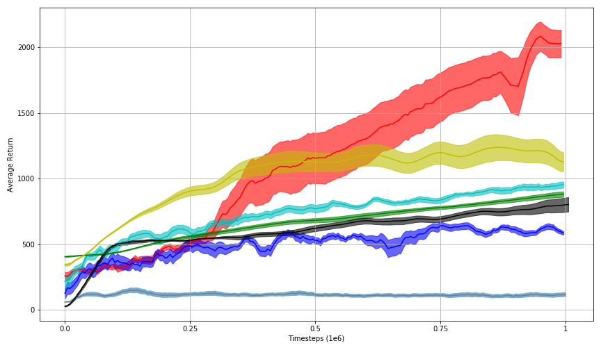
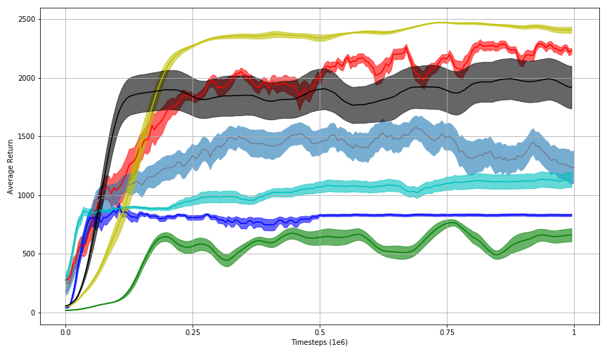
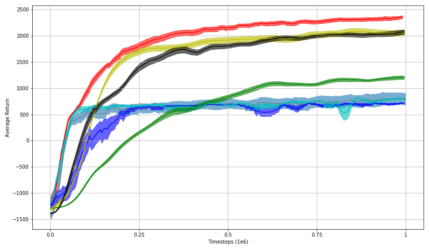
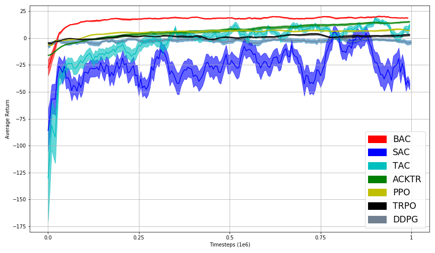
We compare our method to soft actor critic (SAC)(Haarnoja et al., 2018); Tsallis actor-critic (TAC)(Chen and Peng, 2019), a recent off-policy algorithm for learning maximum entropy policies, where we use the implementation of authors ; proximal policy optimization (PPO)(Schulman et al., 2017), a stable and efficient on-policy policy gradient algorithm; deep deterministic policy gradient (DDPG)(Lillicrap et al., 2015); trust region policy optimization (TRPO)(Schulman et al., 2015); and Actor Critic using Kronecker-Factored Trust Region (ACKTR)(Wu et al., 2017), as implemented by OpenAI’s baselines repository . Each task is run for 1 million time steps and the average return of 15 episodes is reported every 5000 time steps. To enable reproducibility, each experiment is conducted on 3 random seeds of Gym simulator and network initialization.

In order for all $\psi$ features to contribute proportionally to the behavior function, it seems convenient to enforce feature scaling since state-action pairs may correspond to a broad range of $\psi$ values. One possible solution is to normalize $\psi$ by considering $\bar{\psi}(s,a)=\frac{\psi(s,a)}{\max\psi(s,a)}$. As a matter of fact, some environments are highly stochastic in terms of transition dynamics which makes learning unstable, not to mention the direct effect of the behavioral Q-function on the scale of gradient that may lead to drastic updates of the policy and even bad convergence. Motivated by this idea, we limit the policy gradient to an appropriate range by a global norm $\mathcal{N}$. Specifically, we applied this technique to HalfCheetah Bullet environment setting $\mathcal{N}=3$.

Table 1: Max Average Return over trials of 1 million time steps. the best performing algorithm for each task is bolded. $\pm$ corresponds to a single standard deviation over trials.

Algorithm	HalfCheetah	Reacher	Ant	Walker2D	Hopper
BAC	2369.15 $\pm$ 104.53	23.42 $\pm$ 0.49	2122.81 $\pm$ 392.34	1814.93 $\pm$ 153.59	2384.24 $\pm$ 111.42
DDPG	830.13 $\pm$ 467.08	1.68 $\pm$ 5.18	177.33 $\pm$ 112.56	586.84 $\pm$ 154.66	1650.68 $\pm$ 392.73
SAC	777.37 $\pm$ 60.5	24.24 $\pm$ 5.56	685.53 $\pm$ 26.49	932.92 $\pm$ 74.06	972.28 $\pm$ 41.23
TAC	844.58 $\pm$ 45.08	25.6 $\pm$ 6.97	974.0 $\pm$ 127.21	1000.54 $\pm$ 1.3	1160.17 $\pm$ 289.93
ACKTR	1210.0 $\pm$ 126.75	14.63 $\pm$ 1.36	830.54 $\pm$ 58.71	642.33 $\pm$ 143.2	754.33 $\pm$ 96.84
PPO	2081.41$\pm$ 251.66	9.05 $\pm$ 1.95	1240.08 $\pm$ 390.54	1231.21 $\pm$ 62.37	2477.98 $\pm$ 16.71
TRPO	2082.81$\pm$ 151.81	4.12 $\pm$ 3.7	806.12 $\pm$ 222.99	1096.48 $\pm$ 224.99	1999.87 $\pm$ 701.62

Our results are shown in Table (1) and learning curves in Figure (1). Based on that, we can deduce that BAC generally outperforms all other algorithms in terms of both final performance and learning speed.

Figure 2: Stochastic vs. Deterministic BAC.

6.2 Stochastic Policy vs Deterministic Policy

In our experiments, behavior-guided actor critic was encouraged to learn a stochastic policy. However, given that our method is not restricted to a specific policy type, it seems tempting to compare the standard BAC to its deterministic variant, where we seek to optimize the objective in Equation (4) by following a deterministic policy. For this sake, we conducted our comparative evaluation on the high dimensional Ant Bullet environment and the experiments were run for 1.5 million steps.

One point worthy of noting is that autoencoders may fail to correctly represent novel and promising state-action pairs if they are in the neighborhood of a frequently visited state-action pair; this may not allow the policy to try all promising paths and lead to slow learning. To fill that gap, we considered adding small noise to the actions selected by the deterministic policy.

Figure (2) shows the superiority of the deterministic variant in terms of stability, but no difference in the final performance when compared to the stochastic BAC meaning that the behavior function is achieving sufficient exploration regardless of the policy type and leading to a state-of-the-art performance along with the proposed architecture of BAC.

6.3 Behavior Temperature

Table (2) shows behavior temperatures $\alpha$ used in our experiments:

Table 2: Temperature parameter

Environment	Hopper	Walker2D	Reacher	Ant	HalfCheetah
Static $\alpha$	0.05	0.04	0.05	0.2	0.03

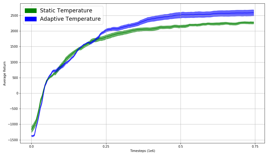
We further explore a variant of BAC that dynamically weights the priority given to the discounted long-term reward function against the behavior function. We make use of a more expressive and tractable approach to endow our method with more efficient exploration and performance while overcoming the brittleness in setting $\alpha$. Specifically, the algorithm follows the performance gradient when it is making progress, and seeks to maximize the behavior function if stuck in a local optimum. To address this issue, consider the weighted objective $J(\pi)$ as following:

Figure 3: Adaptive vs. Static Temperature

$$J(\pi)=\operatorname*{\mathbb{E}}_{s\sim p,a\sim\pi}[\sum_{t_{0}}^{\infty}\gamma^{t}(\alpha r(s_{t},a_{t})+\gamma(1-\alpha)\psi(s_{t+1},a_{t+1}))]$$ (12)

We make use of a neural network $\mathcal{Q}_{\eta}$ ($\mathcal{Q}$ for simplicity) to estimate the quality of an action in a certain state with respect to the policy of interest and future rewards only. Similar to the critic, $\mathcal{Q}$ seeks to minimize the loss $\mathcal{L}=\mathbb{E}[||\mathcal{Q}^{\prime}-\mathcal{Q}||_{2}^{2}]$, where $\mathcal{Q}=\mathcal{Q}(s,g_{\theta}(\epsilon,s))$ and $\mathcal{Q}^{\prime}=r+\gamma\mathcal{Q}(s^{\prime},g_{\theta}(\epsilon,s^{\prime}))$ s.t. $s,s^{\prime}\sim\mathcal{D}$ .

The intuition behind using $\mathcal{Q}$ to come up with a formula of $\alpha$, is that when the distance between $\mathcal{Q}$ and its target is small, the algorithm is not making progress and is probably stuck in a local optimum, and vice versa. We draw an inspiration from this idea to define $\alpha$ as following:

$$\alpha=\sigma\left(\omega\frac{\overline{|\mathcal{Q}-\mathcal{Q}^{\prime}|}-\min|\mathcal{Q}-\mathcal{Q}^{\prime}|}{\max|\mathcal{Q}-\mathcal{Q}^{\prime}|-\min|\mathcal{Q}-\mathcal{Q}^{\prime}|}\right)$$ (13)

where $\sigma$ is the sigmoid function and $\omega=10$ for our convenience. We empirically evaluated this method and compared it to the standard BAC where the experiments were run for 0.75 million steps on HalfCheetah Bullet environment and results were shown in Figure (3).

7 Conclusion

Behavior-guided actor critic is designed to promote exploration and avoid local optima that most recent algorithms struggle with. Specifically, BAC benefits from the discrepancy between the agent-relative representation and the actual features of the state-action pairs to formulate a function that describes the agent’s behavior and consequently maximizes it to avoid getting stuck in a certain region of the solution space. To achieve this, we draw inspiration from various RL frameworks and adopt an off-policy actor critic method to optimize the conventional RL objective along with the behavior function. We also provide theoretical analysis and prove that our method converges to the optimal policy allowing us to formalize the BAC algorithm. BAC has shown high competence and proved to be a competitive candidate to solve challenging, high-dimensional RL tasks. Our method can also be extended to various learning frameworks. We believe that investigating the relative importance $\alpha$ of the behavior function and finding an adaptive schedule would be fruitful to consider in future works.

8 Broader Impact

This work does not currently present any foreseeable societal consequence.

References

- Araya et al. (2012) Araya, M., Buffet, O., and Thomas, V. (2012). Near-optimal brl using optimistic local transitions. arXiv preprint arXiv:1206.4613.
- Bellemare et al. (2016) Bellemare, M. G., Srinivasan, S., Ostrovski, G., Schaul, T., Saxton, D., and Munos, R. (2016). Unifying count-based exploration and intrinsic motivation. In 30th Conference on Neural Information Processing Systems.
- Brafman and Tennenholtz (2002) Brafman, R. I. and Tennenholtz, M. (2002). R-max-a general polynomial time algorithm for near-optimal reinforcement learning. Journal of Machine Learning Research, 3(Oct):213–231.
- Brockman et al. (2016) Brockman, G., Cheung, V., Pettersson, L., Schneider, J., Schulman, J., Tang, J., and Zaremba, W. (2016). Openai gym. arXiv preprint arXiv:1606.01540.
- Burda et al. (2018) Burda, Y., Edwards, H., Pathak, D., Storkey, A., Darrell, T., and Efros, A. A. (2018). Large-scale study of curiosity-driven learning. arXiv preprint arXiv:1808.04355.
- Chen and Peng (2019) Chen, G. and Peng, Y. (2019). Off-policy actor-critic in an ensemble: Achieving maximum general entropy and effective environment exploration in deep reinforcement learning. arXiv preprint arXiv:1902.05551.
- Conti et al. (2018) Conti, E., Madhavan, V., Such, F. P., Lehman, J., Stanley, K. O., and Clune, J. (2018). Improving exploration in evolution strategies for deep reinforcement learning via a population of novelty-seeking agents. In 32nd Conference on Neural Information Processing Systems.
- Degris et al. (2012) Degris, T., White, M., and Sutton, R. S. (2012). Off-policy actor-critic. arXiv preprint arXiv:1205.4839.
- Doshi-Velez et al. (2010) Doshi-Velez, F., Wingate, D., Roy, N., and Tenenbaum, J. B. (2010). Nonparametric bayesian policy priors for reinforcement learning. In Advances in Neural Information Processing Systems, pages 532–540.
- Fujimoto et al. (2018) Fujimoto, S., Van Hoof, H., and Meger, D. (2018). Addressing function approximation error in actor-critic methods. arXiv preprint arXiv:1802.09477.
- Geist and Pietquin (2010) Geist, M. and Pietquin, O. (2010). Managing uncertainty within value function approximation in reinforcement learning. In Active Learning and Experimental Design workshop (collocated with AISTATS 2010), Sardinia, Italy, volume 92.
- Goodfellow et al. (2016) Goodfellow, I., Bengio, Y., and Courville, A. (2016). Deep Learning. MIT Press. http://www.deeplearningbook.org.
- Haarnoja et al. (2018) Haarnoja, T., Zhou, A., Abbeel, P., and Levine, S. (2018). Soft actor-critic: Off-policy maximum entropy deep reinforcement learning with a stochastic actor. In 35th International Conference on Machine Learning.
- Jaksch et al. (2008) Jaksch, T., Ortner, R., and Auer, P. (2008). Near-optimal regret bounds for reinforcement learning. J. Mach. Learn. Res., 11:1563–1600.
- Kearns and Singh (2004) Kearns, M. and Singh, S. P. (2004). Near-optimal reinforcement learning in polynomial time. Machine Learning, 49:209–232.
- Kingma and Welling (2013) Kingma, D. P. and Welling, M. (2013). Auto-encoding variational bayes. arXiv preprint arXiv:1312.6114.
- Kolter and Ng (2009) Kolter, J. Z. and Ng, A. Y. (2009). Near-bayesian exploration in polynomial time. In 26th International Conference on Machine Learning.
- Lang et al. (2012) Lang, T., Toussaint, M., and Kersting, K. (2012). Exploration in relational domains for model-based reinforcement learning. J. Mach. Learn. Res., 13:3725–3768.
- Lillicrap et al. (2015) Lillicrap, T. P., Hunt, J. J., Pritzel, A., Heess, N. M. O., Erez, T., Tassa, Y., Silver, D., and Wierstra, D. (2015). Continuous control with deep reinforcement learning. CoRR, abs/1509.02971.
- Lopes et al. (2012) Lopes, M., Lang, T., Toussaint, M., and Oudeyer, P.-Y. (2012). Exploration in model-based reinforcement learning by empirically estimating learning progress. In 26th Conference on Neural Information Processing Systems.
- Mnih et al. (2015) Mnih, V., Kavukcuoglu, K., Silver, D., Rusu, A. A., Veness, J., Bellemare, M. G., Graves, A., Riedmiller, M. A., Fidjeland, A. K., Ostrovski, G., Petersen, S., Beattie, C., Sadik, A., Antonoglou, I., King, H., Kumaran, D., Wierstra, D., Legg, S., and Hassabis, D. (2015). Human-level control through deep reinforcement learning. Nature, 518:529–533.
- Ostrovski et al. (2017) Ostrovski, G., Bellemare, M. G., van den Oord, A., and Munos, R. (2017). Count-based exploration with neural density models. ArXiv, abs/1703.01310.
- Pathak et al. (2017) Pathak, D., Agrawal, P., Efros, A. A., and Darrell, T. (2017). Curiosity-driven exploration by self-supervised prediction. 2017 IEEE Conference on Computer Vision and Pattern Recognition Workshops (CVPRW), pages 488–489.
- Schmidhuber (2006) Schmidhuber, J. (2006). Developmental robotics, optimal artificial curiosity, creativity, music, and the fine arts. Connection Science, 18:173 – 187.
- Schulman et al. (2015) Schulman, J., Levine, S., Abbeel, P., Jordan, M. I., and Moritz, P. (2015). Trust region policy optimization. In 32nd International Conference on Machine Learning.
- Schulman et al. (2017) Schulman, J., Wolski, F., Dhariwal, P., Radford, A., and Klimov, O. (2017). Proximal policy optimization algorithms. arXiv preprint arXiv:1707.06347.
- Sorg et al. (2010) Sorg, J., Singh, S. P., and Lewis, R. L. (2010). Variance-based rewards for approximate bayesian reinforcement learning. In 26th Conference on Uncertainty in Artificial Intelligence.
- Strehl and Littman (2008) Strehl, A. L. and Littman, M. L. (2008). An analysis of model-based interval estimation for markov decision processes. J. Comput. Syst. Sci., 74:1309–1331.
- Tan et al. (2018) Tan, J., Zhang, T., Coumans, E., Iscen, A., Bai, Y., Hafner, D., Bohez, S., and Vanhoucke, V. (2018). Sim-to-real: Learning agile locomotion for quadruped robots. arXiv preprint arXiv:1804.10332.
- Tang et al. (2017) Tang, H., Houthooft, R., Foote, D., Stooke, A., Chen, X., Duan, Y., Schulman, J., Turck, F. D., and Abbeel, P. (2017). #exploration: A study of count-based exploration for deep reinforcement learning. In 31st Conference on Neural Information Processing Systems.
- Todorov et al. (2012) Todorov, E., Erez, T., and Tassa, Y. (2012). Mujoco: A physics engine for model-based control. In 2012 IEEE/RSJ International Conference on Intelligent Robots and Systems, pages 5026–5033. IEEE.
- van Hasselt (2010) van Hasselt, H. (2010). Double q-learning. In 24th Conference on Neural Information Processing Systems.
- Wu et al. (2017) Wu, Y., Mansimov, E., Grosse, R. B., Liao, S., and Ba, J. (2017). Scalable trust-region method for deep reinforcement learning using kronecker-factored approximation. ArXiv, abs/1708.05144.