Fast, Smart Neuromorphic Sensors Based on Heterogeneous Networks and Mixed Encodings

Abstract

Neuromorphic architectures are ideally suited for the implementation of smart sensors able to react, learn, and respond to a changing environment. Our work uses the insect brain as a model to understand how heterogeneous architectures, incorporating different types of neurons and encodings, can be leveraged to create systems integrating input processing, evaluation, and response. Here we show how the combination of time and rate encodings can lead to fast sensors that are able to generate a hypothesis on the input in only a few cycles and then use that hypothesis as secondary input for more detailed analysis.

I Introduction

Smart sensors is one of the areas in which neuromorphic computing can be transformational: the ability to build compact systems able to react, learn, adapt, communicate, and remember while immersed in a changing, unpredictable environment could find applications across many domains. Insects provide an ideal model system for the exploration of neuromorphic architectures that can act as smart sensors. A species such as Drosophila is able to process and integrate multiple inputs, exhibit short and long term memory, and display a variety of learning behaviors, all while being proficient while airborne. This range of behavior is achieved with a comparatively small number of neurons, 100,000 in the case of Drosophila,[1] and fast response times. For instance, olfactory receptor neurons can resolve input fluctuations at more than 100 Hz.[2]

It is not unreasonable to assume that, should we had a better understanding of the design principles underlying the insect’s brain, the fabrication of chips implementing such complex functionality would be within the reach of our current device fabrication capabilities. The possibility of implementing complex systems with a relatively few neurons also broadens the range of platforms that could be employed to manufacture such sensors. Examples include large ($\geq 90$ nm) technology nodes or wide bandgap semiconductors such as SiC for operation under extreme environments, and the use of TFT or printing and additive manufacturing technologies.[3, 4]

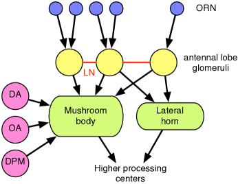
Figure 1: Scheme of the olfactive processing pathway on higher insects. Despite its small size, the arthropod brain is highly modular: inputs from the antennal lobes project into two separate pathways: the lateral horn, responsible of innate responses, and the mushroom body, one of the key centers for memory and learning in the insects. Learning in the mushroom body is modulated by independent modulatory circuits.

However, despite having various orders of magnitude fewer neurons than mammals, the insect brain is remarkably heterogeneous. It is is composed of a number of well-differentiated functional structures, with clear parallelisms with the much larger mammal brain. [5] An example is provided in Figure 1, where we show a functional model of the olfactory processing and learning subsystem of Drosophila melanogaster. It also exhibits multiple types of neurons, neurotransmitters and neuromodulators, [1] as well as multiple encodings: population, sparse, spike timing, and single spike codes have all been experimentally observed. [6, 7] Recent studies also suggest that dynamic plasticity can be associated with a small subset of neurons, providing yet another source of heterogeneity.[8, 9]

Understanding the behavior of such heterogeneous systems, and in particular the way in which different components can be integrated to achieve a desired functionality, can help accelerate the development of standalone neuro-inspired smart sensors, as well as neuromorphic systems in general. This knowledge can also inform the design and fabrication of neuromorphic systems from a hardware perspective: the choices that we make building such a system, from standard vs custom ASIC chips down to spiking vs non-spiking, analog vs digital, CMOS vs memristive-based, and standard vs novel materials choices in novel architectures, can have a strong impact in the ultimate performance and capabilities in ways that are not yet fully understood.

This manuscript is structured as follows: in Section II, we introduce our approach to integrate spiking neurons with non-spiking recurrent neurons, and we introduce the types of architectures that are the focus of our study. In Section III-A we validate that the state based representation of spiking neurons provides an accurate description of spiking neurons. We then use this model in Section III-B to explore different types of encodings, and compare their pattern recognition capabilities using the same network. In Sections III-C and III-D we focus on the sparse coding approach enabled by the mushroom body type of architectures. We also show how this type of architecture provides the ideal substrate for implementing online modulatory learning. Finally, we discuss the implications that our results have on the design and choice of neuromorphic hardware.

II Model

II-A Integration of spiking and non-spiking neural networks

A central aspect of our model is the integration of spiking and non-spiking neural neurons. Our approach was to develop a synchronous, recurrent, yet accurate representation of a leaky integrate and fire model.

Our starting point is the standard leaky integrate and fire model:[12]

$$\tau\frac{dv_{i}}{dt}=-v_{i}+\sum_{j}w_{ji}\delta(t-t_{j})+v_{\mathrm{ext}}^{(i)}$$ (1)

subject to the spiking condition:

$$v_{i}(t)=1\Rightarrow v_{i}(t+t^{\prime})=0\hskip 14.22636pt\forall\hskip 14.22636ptt^{\prime}<\tau_{r}$$ (2)

where $\tau_{r}$ is an absolute refractory period.

We can take advantage of the fact that for any $\Delta t\leq\tau_{r}$ we can have at least one spike to integrate over $\Delta t$ and express the output of each neuron as a binary variable $s_{i}=0,1$ at each interval. In order to transform the firing times $t_{j}$ of the neurons projecting into our neuron into time steps $n_{i}$, so that $n_{j}\Delta t\geq t_{j}<(n_{j}+1)\Delta t$, we assume that $t_{j}$ is homogeneously distributed within that interval: $P(t_{j})=\frac{1}{\Delta t}$. This approximation, which is equivalent to assuming that we lose any information below our time scale $\Delta t$, allows us to formulate Eq. 1 as:

$$\begin{array}[]{lcl}v_{i}(n)&=&(1-s_{i}(n-1))\left[\xi_{i}(n)\left(1-e^{-1/\tau_{m}}\right)\right.\\ &&+\left.v_{i}(n-1)e^{-1/\tau_{m}}\right]\\ &&+s_{i}(n-1)\xi_{i}(n)\left(1-\tau_{m}(1-e^{-1/\tau_{m}})\right)\\ s_{i}(n)&=&H(v_{i}(n)-v_{0i})\\ \xi_{i}(n)&=&v_{\mathrm{ext}}^{(i)}+\sum_{j}\frac{w_{ji}}{\tau_{r}}s_{j}(n-n_{ji})\end{array}$$ (3)

Here $s_{i}=0,1$ depending on whether the neuron is spiking on a given time step, $v_{i}$ is the membrane potential, $\tau_{m}$ is the neuron time constant normalized to the absolute refractory period, and $H(\cdot)$ is the Heaviside or step function. The presence of two terms, one proportional to $(1-s_{i})$ and another to $s_{i}$, in Eq. 3 comes from the need of considering the impact of the absolute refractory period on the evolution of the membrane potential $v_{i}$: if the neuron spiked in the prior interval, the increase in potential will be lower for the same total input since the neuron is active only during a fraction of the time.

If we neglect the impact of the refractory period that we just mentioned from Eq. 3, the recurrence relation for $v_{i}$ simplifies to:

$$\begin{array}[]{lcl}v_{i}(n)&=&\left(1-e^{-1/\tau_{m}}\right)\xi_{i}(n)\\ &&+\left((1-s_{i}(n-1)\right)v_{i}(n-1)e^{-1/\tau_{m}}\\ s_{i}(n)&=&H(v_{i}(n)-v_{0i})\\ \xi_{i}(n)&=&v_{\mathrm{ext}}^{(i)}+\sum_{j}\frac{w_{ji}}{\tau_{r}}s_{j}(n-n_{ji})\end{array}$$ (4)

Eq. 4 represents a recurrent version of the classic McCulloch-Pitts model. [13] If we can neglect the memory effect on the neuron the classic model is recovered.

We can use Eq. 3 as a starting point to implement a training algorithm based on the stochastic gradient descent method. In order to do that, we simply replace the Heaviside function in Eq. 3 by a differentiable activation function $a_{i}$. Here, we use the logistic function $\sigma(\cdot)$ weighed by a factor $\beta$ used to control the sharpness of the transition, so that:

$$a_{i}=\sigma(\beta(v_{i}-v^{(i)}_{0}))$$ (5)

The resulting equation is non-linear in $a_{i}$ due to the presence of the $(1-s_{i})$ and $s_{i}$ factors mentioned in the previous section.

II-B Architecture

In this work we have focused on the architecture shown in Figure 2. This design is clearly inspired on one of the memory and learning centers in the insect brain shown in Figure 1. [8, 14]

We consider systems composed of two parallel pathways for input processing [Figure 2(A)]. A fast component contains innate information that is processed using a neural network based on either single spike, spike timing, or rate encoding. This structure is an abstraction from the lateral horn in the insect brain.

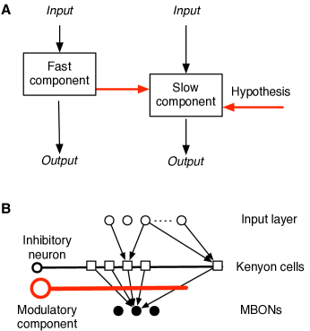
Figure 2: Scheme of the olfactive processing pathway on a higher insects. Inputs from the antennal lobes project into two separate pathways: the lateral horn, responsible of innate responses, and the mushroom body, one of the key centers for memory and learning in the insects. The mushroom body is modulated by modulatory circuits.

In a second pathway, we have a fan-out fan-in network for sparse encoding of information [Figure 2(B)]. [15] The input data projects into a set of identical neurons (Kenyon cells) that are sparsely connected. The connectivity is randomly determined so that only a fraction of input neurons feed into each Kenyon cells. These cells can be recurrently connected. The sparsity of neural activity is maintained through a single inhibitory neuron that receives input from and connects to every Kenyon cell. The Kenyon cells project into an output layer (mushroom body output neurons - MBONs). Only the synaptic weights between the Kenyon cells and the output neurons are plastic.[14] The rest of synapses are kept constant during the offline or online training.

II-C Modulation as enabler of state or hypothesis-dependent learning

A key component of biological systems is the ability to decide when to learn and when not to learn. In the insect brain, clusters of modulatory neurons implement such capability though modulatory learning.[8, 9] If in spike timing dependent plasticity the synaptic strength $W_{\mathrm{AB}}$ between two neurons A and B is a function of their activity: $W_{\mathrm{AB}}=f(\mathrm{A},\mathrm{B})$, in the case of modulated learning, the synaptic strength is a function of the pre-synaptic neuron and a third neuron C: $W_{\mathrm{AB}}=f(\mathrm{A},\mathrm{C})$, and optionally the post-synaptic neuron as well. This provides a substrate to integrate logic and memory through dynamic plasticity: we can actuate learning or strengthen certain pathways by the action of a third input. Details on how to implement such functionality from a hardware perspective will be shown elsewhere.

III Results

III-A The state model of spiking neurons is functionally equivalent to the LIF model for sparse activity

In order to understand the impact of our synchronous approximation to a leaky integrate and fire model, we have compared the activity pattern of our model and asynchronous model for a series of randomly connected networks subject to a random set of inputs. In Figure 3 we show the correlation between the activity of a leaky integrate and fire modeled following equation 1 and its corresponding state representation given by Eq. 3. .

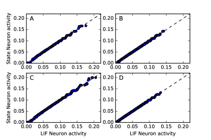
Figure 3: Correlation between the standard LIF model and the state model of a spiking neuron used in this work

The correlation between the two models is excellent, indicating that the loss of information of the exact firing times does not negatively impact its functionality for a broad set of conditions. In particular, this allows us to extract the lessons from prior exhaustive studies on the leaky integrate and fire neurons to a recurrent, synchronous model.[12]

III-B Comparison between different encodings: MNIST benchmarks

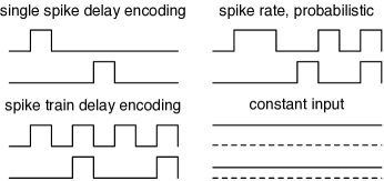
Figure 4: Different encodings implemented in this work

In order to explore the ability of different encodings to learn and discriminate between different inputs we have used the state model introduced above to benchmark the performance of a shallow network against the MNIST dataset. We have considered the following four types of encoding (Figure 4):

1. Single spike delay encoding. In this case the input is codified as a single spike whose delay with respect to a common epoch decreases with the input intensity.

2. Spike train delay encoding. The single spikes from the time encoding are subsequently followed by a periodic train of spikes spaced by an interval equal to the time delay.

3. spike rate, probabilistic. The spiking neurons are fed a constant input proportional to the intensity of each pixel in the input data.

4. Constant analog input. The input is codified as constant input signal.

For each of the proposed encodings, we applied a stochastic gradient descent method to optimize our networks using a cost function that optimized the total number of spikes:

$$C=\frac{1}{N}\sum_{i}\left(\sum_{m}a_{i}(m)-n_{i}\right)^{2}$$ (6)

regardless of when those spikes took place.

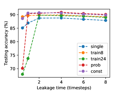
Figure 5: MNIST accuracy of a shallow spiking neural network as a function of the neuron leakage time for various encodings. single: single spike delay; train8: spike train delay encoding, 8 time steps; train24: spike train delay encoding, 24 time steps; prob: probabilistic spike rate; const: constant input

In Figure 5 we show the testing accuracy for the encodings considered after being trained against 180,000 randomly selected images from MNIST’s training set. The results are shown as a function of the characteristic time of the neurons $\tau_{m}$. Low values of $\tau_{m}$ correspond to short-term memory neurons that emphasizes the contributions within a given interval. The results show testing accuracies as high as 90%. This compares well with state of the art results for shallow (no hidden layers) neural networks.[16] In particular, if we optimize a shallow network of non-spiking sigmoidal neurons using the same cost function and stochastic gradient descent method, the resulting accuracy is 91%.

TABLE I: MNIST test accuracy: comparison between sigmoidal and binary outputs for multiple encodings

Encoding	Sigmoidal	Binary non-excl.	Binary excl.
Single spike delay	88%	83%	65%
Spike train delay	90%	90%	87%
Spike rate, prob	91%	91%	87%
Constant	88%	83%	65%

Overall, the conclusions of this analysis is that the learning capability of spiking neurons is similar to that of non-spiking neurons, at least in the context of the MNIST dataset. Moreover, even in the case of a spike rate, the testing accuracy is fairly insensitive to the sampling length. In this particular case, a testing accuracy of 90% is achieved in only eight steps.

The results obtained in Figure 5 are obtained by changing the binary output of the neuron by a steep sigmoidal function. If we switch back to a binary output, the differences between the different encodings become more pronounced. The results are summarized in Table I. The non-exclusive accuracy column includes all cases where the correct digit achieves the maximum number of spikes, regardless of whether other digits also achieves the same number of spikes. In contrast, the exclusive accuracy column considers only those cases where no other digits achieve the maximum number of spikes. The need to distinguish between these to cases comes from the fact that the output is measured in terms of the number of spikes, so two neurons can have identical outputs. According to the results obtained, the single spike encoding’s testing (exclusive) accuracy drops below 70%. In contrast, both the spike train time delay and the probabilistic spike rate encodings maintain a high testing accuracy with binary outputs.

III-C Sparse encoding using mushroom body architectures

The fan-out fan-in architecture of the mushroom body shown in Figure 2 casts the input into a higher dimensional space, with learning taking place solely in the fan-in part of the network. The number of Kenyon cells $N$ and the number random connections $n_{c}$ of the Kenyon cells are the two key structural variables.

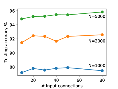
Figure 6: MNIST testing accuracy for a mushroom body fan-out fan-in type of architecture as a function of both the number of Kenyon cells $N$ and the number of input connections $n_{c}$

In order to understand the role of each of them in pattern recognition tasks, we have trained a mushroom body type of network against the MNIST dataset. The results presented in Figure 6 show that the number of Kenyon cells, that is, the dimensionality of the fan-out parameter, is the critical variable controlling testing accuracy. In contrast, the number of random connections $n_{c}$ has a second order influence. Note that the results obtained in Figure 6 were obtained using the same metalearning parameters of the stochastic gradient descent method using ramdom fan-out connectivity. Consequently, there is the possibility that higher accuracies could be obtained in some cases through a better choice of these parameters. In the case of 5000 Kenyon cells, the mushroom body type of architecture was able to achieve 95% testing accuracies.

Similar to the studies shown in the prior section, we can implement the same type of network using spiking neurons. These neurons were modulated by an inhibitory network as explained in the prior section. When subject to a spike train encoding of input data it results on a complex sparse activity pattern due to the strong inhibitory component. One such example is shown in Figure 7 for one of the images of the MNIST training set for a network composed of 1000 Kenyon cells, each receiving the input of 70 randomly selected data streams.

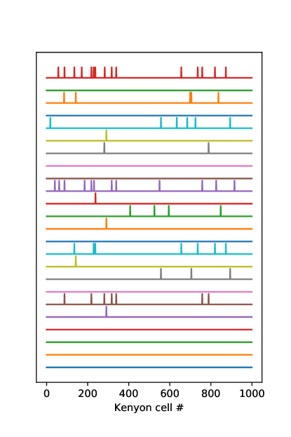
Figure 7: Neuron activity as a function of Kenyon cell # over 24 intervals after receiving a MNIST digit codified using a time delay + spike train encoding input. The presence of an inhibitory neuron enhances the sparsity of the response both in time and over the range of active Kenyon cells. No recurrent interactions among Kenyon cells was considered for this example.

When the output of the Kenyon cells is fed to an output layer of spiking neurons using a rate encoding, we can use stochastic gradient descent methods to optimize the response of the output layer. The resulting testing accuracy again exceeds 89%, as shown in Figure 8. When we combine a time encoding with sparse encoding, the joint accuracy of the combined system is 95%. The fast evaluation through time encoding is carried out in only 8 time cycles, whereas for the mushroom body we considered the output rate after 24 cycles.

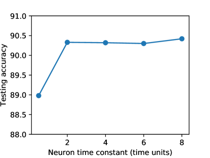
Figure 8: MNIST accuracy of a mushroom body-inspired network containing 1000 Kenyon cells, each receiving 70 randomly selected inputs. Kenyon cell rates over 24 periods are used to fit an output layer of spiking neurons. Results are shown for output neurons with different neuron time constants $\tau_{m}$

III-D The mushroom body architecture provides a substrate for online associative learning and hypothesis-driven perception

A key advantage of the fan-out fan-in architecture is that it provides a substrate for on-line associative learning. So far all the approaches used in Section III-B rely on the use of stochastic gradient descent methods to train the network for a particular task. In the fan-out fan-in architecture we can use modulatory signals to establish associations between certain activity patterns and a desired output.

One such example is the redirection of the output of the fast component to help the Kenyon cell learn patterns online. This provides a simple way of loading information into the slow, plastic component only as it is presented or required by the system. Another example is the use of the fast component to modulate a probabilistic interpretation of the input. One such example is shown in Figure 9, where the a priori probabilistic assumption of the input increases the ability of the system to enhance the testing accuracy of a fan out architecture optimized using modulated plasticity.

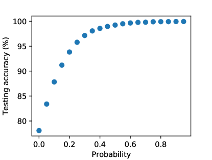
Figure 9: Modulation of MNIST testing accuracy on a mushroom body type of architecture as a function of prior knowledge

A more compelling example is to use this modulatory component to change the behavioral output of a system. Here we show an agent carrying out a random walk on a 2D space receiving a series of spatially correlated input data. For this particular example we consider a series of point sources randomly distributed over a 2D map (Figure 10). These sources emit a particular combination of input data. These can be interpreted as either specific set of pulses or frequencies, in the case of radio or visual navigation, or it can be series of molecular signals. We consider that the intensity of these pulses decay with distance following a gaussian profile.

The network is composed of 20 input neurons, 200 Kenyon cells and one output neuron signaling the valence of the input. The agent carries out a random walk over the map with a dwell time that is modulated by the valence associated to the input (Figure 10). A positive valence leads to longer dwell times during the random walk. In absence of modulatory input, the dwell time is homogeneously distributed on the map. In order to train the system to spend more time at the center of the map, we introduced a modulatory signal that strengthen the positive response with a certain probability $p_{0}$ whenever the agent is within a certain region. A feedback path ensures that, once the system has learned the desired response, the modulatory neuron becomes inactive and the synaptic weights are no longer updated.

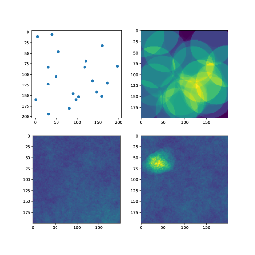
Figure 10: Aggregated dwell times of an agent carrying out a random walk over a 2D map. Top left: spatial distribution of source points providing the input of the system. Top right: fraction of action Kenyon cells as a function of the position. Bottom left: Dwell time distribution in absence of reinforcement. Bottom right: Dwell time distribution after on-line reinforcement of the central position of the map, showing an increase of dwell time close of the excitation area in the top left quadrant.

IV Discussion and conclusions

The results obtained allow us to extract some useful lessons from a hardware perspective: first, they indicate that the learning capabilities of different types of encodings in spiking neural networks do not significantly differ from the traditional non-spiking counterparts. Moreover, we showed how both using random spike rate and deterministic spike train encodings it was possible to achieve similar MNIST testing accuracies in as few as eight time steps. This suggests that results obtained in the literature using random spike trains could be reproduced using deterministic spike rates in hardware as long as the characteristic response time of the neuron is larger than a single time step. From a sensing and processing point of view, this implies that spiking systems could process information in a few clock cycles per layer even when a spike rate encoding is used.

Second, the exploration of sparse coding in fan-out fan-in architectures inspired in the insect’s mushroom body shows that these systems achieve both good testing accuracy and the ability to carry out online learning. An interesting feature of such systems is that, similar to liquid state machines, learning only takes place in the fan-in region. [17] Consequently, this type of architecture is amenable to a modular design, where the online/dynamic plasticity component is contained within a separate module. They are also compatible with existing hardware approaches.

Finally, modulatory learning provides an effective approach for implementing online associative learning that is conditional to an internal state or external command. The central idea is that the synaptic strength between two neurons is mediated by a third neuron, bringing together the logic and learning aspects of neural systems. While the focus of this work was not on devices, we have emulated such modulatory learning using both memristors and CMOS-based approaches.

References

- [1] A.-S. Chiang, C.-Y. Lin, C.-C. Chuang, et al, Current Biology, 21, 1, 2011)
- [2] P. Szyszka, R. C. Gerkin, C. G. Galizia, and B. H. Smith, Proceedings of the National Academy of Sciences, 111, 16 925, 2014.
- [3] E. Fortunato, P. Barquinha, and R. Martins, Advanced Materials 24, 2945, 2012.
- [4] P. G. Neudeck, R. D. Meredith, L. Chen, et al, AIP Advances, 6, 125119, 2016.
- [5] N. J. Strausfeld and F. Hirth, Science, 340, 157, 2013.
- [6] M. Joesch, J. Plett, A. Borst, and D. F. Reiff, Current Biology, 18, 368, 2008.
- [7] J. Perez-Orive, O. Mazor, G. Turner, et al, Science, 297, 359, 2002
- [8] Y. Aso, D. Sitaraman, T. Ichinose, et al, eLife, 3, e04580, 2014.
- [9] Y. Aso, D. Hattori, Y. Yu, et al, eLife, 3, e04577, 2014.
- [10] S. B. Furber, F. Galluppi, S. Temple, and L. A. Plana, Proceedings of the IEEE, 102, 652, 2014.
- [11] S. K. Esser, P. A. Merolla, J. V. Arthur, et al, PNAS, 113, 11 441, 2016.
- [12] N. Brunel, Journal of Computational Neuroscience, 8, 183, 2000.
- [13] W. S. McCulloch and W. Pitts, The bulletin of mathematical biophysics, 5, 115, 1943.
- [14] T. Hige, Y. Aso, M. N. Modi, G. M. Rubin, and G. C. Turner, Neuron, 88, 985, 2015.
- [15] M. García-Sanchez and R. Huerta, Journal of Computational Neuroscience, 15, 5, 2003.
- [16] Y. Lecun, L. Bottou, Y. Bengio, and P. Haffner, Proceedings of the IEEE, 86, 2278, 1998.
- [17] W. Maass, T. Natschlager, and H. Markram, Neural Computation, 14, 2531, 2002.