Emergent Replica Conformal Symmetry in Non-Hermitian SYK2 Chains
Abstract
Recently, the steady states of non-unitary free fermion dynamics are found to exhibit novel critical phases with power-law squared correlations and a logarithmic subsystem entanglement. In this work, we theoretically understand the underlying physics by constructing solvable static/Brownian quadratic Sachdev-Ye-Kitaev chains with non-Hermitian dynamics. We find the action of the replicated system generally shows (one or infinite copies of) symmetries, which is broken to by the saddle-point solution. This leads to an emergent conformal field theory of the Goldstone modes. We derive the effective action and obtain the universal critical behaviors of squared correlators. Furthermore, the entanglement entropy of a subsystem with length corresponds to the energy of the half-vortex pair , where is the total stiffness of the Goldstone modes. We also discuss special limits with more than one branch of Goldstone modes and comment on interaction effects.
1 Introduction
Under unitary evolution, local quantum information of a generic closed many-body system goes through the process of scrambling and disperses into the entire system. It has long been known that such a process is closely related to thermalization, in which the entanglement entropy of a small subsystem approaches thermal entropy with volume law scaling [1, 2]. Ever since then, systems that evade quantum thermalization have been of special interest. Several mechanisms have been proposed in an effort to realize such systems, including many-body localization [3, 4], prethermalization [5, 6], and non-unitary evolution.
Among these mechanisms, the non-unitary evolution is especially natural since all experimental systems are inevitably open [7]. In a unitary dynamics under repeated measurement, if we follow the quantum trajectories, the steady state is non-thermal and can exhibit entanglement phase transition from a volume law phase to an area law phase [8, 9, 10, 11, 12, 13, 14, 15, 16, 17, 18, 19, 20, 21, 22, 23, 24, 25]. The underlying mechanism also applies to other non-unitary dynamics that host exotic non-thermal phases [26, 27, 28, 29, 30, 31, 32]. For instance, in free fermion non-unitary systems, it is shown that a stable critical phase exists, in which the entanglement entropy is logarithmic in the subsystem size and the correlation functions in the spatial direction exhibit power-law decay [25, 33, 34, 35]. While these results have been corroborated in numerous numerical simulations, concrete solvable models, in which the entanglement entropy and correlation function can be determined analytically, are still lacking and will prove valuable in the understanding of the intimate relation between quantum thermalization and non-Hermiticity.
The Sachdev-Ye-Kitaevq (SYKq) models [36, 37, 38] describe randomly interacting Majorana fermions with infinite-range -fermion interactions. It is found to be solvable in the large- limit where the entanglement entropy and its quench dynamics can be studied [39, 40, 41, 42, 43, 44, 45, 35, 46]. Based on the original SYK model, different generalizations have been constructed. In particular, SYK chains (i.e. coupled SYK dots) have been proposed to understand various dynamical problems in 1D [47, 48, 49, 50, 51, 52, 53]. In [54, 55], the authors further consider introducing the temporal randomness into the SYK model, where the static random interaction terms are replaced by Markovian random interactions. This is known as the Brownian SYK model, which is an analogy of the Brownian circuit models [56, 57, 58, 59, 60, 55, 61].
In this work, combining ideas of non-Hermiticity and the SYK models, we construct a set of concrete non-Hermitian SYK2 chains. We derive the dynamical properties of the steady states in the large- limit. By analyzing the saddle-point equation, we explicitly show that for generic values of the coupling parameters, the replicated system exhibits a replica conformal symmetry due to the existence of Goldstone modes [62]. We demonstrate that the Goldstone modes can be probed by the squared correlator, which features the universal critical scaling. We then argue that the entanglement entropy for a subsystem with length corresponds to the energy of a half-vortex pair [25], given by , where is the stiffness of the Goldstone mode [63, 64]. We finally comment that when the interaction is added, the Goldstone mode acquires a mass, leading to volume-law scaling in the entanglement entropy, which can again be understood from a domain wall picture.
2 Model and setup
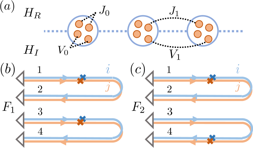
We consider the non-Hermitian SYK2 chain with a Hamiltonian written in terms of
| (1) | ||||
Here labels the Majorana modes on each site. The total Hamiltonian for the chain reads . Random hopping parameters , , , are independent Gaussian variables with zero expectation values. We first focus on the case of static correlations and take their variances as
| (2) | ||||
The case of Brownian correlations will be considered in the Appendix C.
We aim to understand the steady states under the non-Hermitian dynamics. We consider preparing the system in some initial state . For a given disorder configuration, at time , the system is in the state
| (3) |
We are interested in understanding the emergence of the criticality in the non-unitary dynamics [35, 65]. A natural object to study is the Keldysh equal-time two-point function
evaluated on the steady state with . However, in random systems, the disorder averaged correlator vanishes, and we should instead consider the disorder averaged squared correlators. We define two types of squared correlators as
These correlators measure the fluctuation of two-point functions over disorder realizations.
The computation of the correlation functions for disordered quantum systems generally requires the introduction of additional disorder replicas. However, for the SYK-like models in the large- limit, the saddle point solution is diagonal in the disorder replicas [37, 66, 67]. Consequently, and can be represented as four-point functions on the replicated partition function in a single disorder replica:
| (4) |
In the path-integral formulation of , there are four branches of the evolution contour, as shown in FIG. 1 (b-c). We label these four branches by - where the evolution is forward on and backward on . Following the standard SYK derivation, the system is described by a bilocal - action (see Appendix A), which can then be treated within the saddle-point approximation. The effective action that governs the fluctuations around the saddle point can be subsequently derived, which allows to determine the squared correlators analytically. Moreover, the entanglement calculation can be viewed as introducing defects on the boundary of the contour at time . They excite the fluctuations with an energy increase equal to the entanglement entropy.
3 Saddle point and symmetry
We begin with analyzing the saddle-point equation. From now on, we keep the Majorana index implicitly. For SYK-like models, the saddle-point equation is equivalent to the Schwinger-Dyson equation for with labeling Majorana fields on different branches of the contour. Viewing as a matrix in both branch and time space, we have
| (5) |
For our static model, the self-energy reads
| (6) | ||||
this equation contains large symmetries which are rotations between the or branches. To see this, we define the Fourier transformation as . The Schwinger-Dyson equation is then invariant under , with , here is a matrix in the branch space. Consequently, there are infinite copies of the symmetry, labeled by the frequency . Similar symmetry appears when computing the spectral form factor [68]. We note that there is an additional time-reversal symmetry under and [69].
Now we present the solution of the saddle-point equation away from the boundary or . Assuming sufficiently large , such that the system reaches the steady state and the Green’s function becomes translationally invariant in both space and time directions [70]. Since the branches decouple from the branches , we expect to be block diagonal with and for [71]. In the low-energy limit , reads
| (7) | ||||
together with and . Here we have defined , . For , we instead have
| (8) | ||||
For each frequency , the solutions (7) break the symmetry but preserve the time-reversal symmetry. The solutions are only invariant under the symmetry transformation when . We denote the residue symmetry group by , where the subscript represents the generator is . The Goldstone mode lives in the coset space space and is given by . In terms of the original bilocal fields, they correspond to . Here we have defined the fluctuation of fields as . This suggests there should be a line of Goldstone modes labeled by frequency . Similar physics has also been observed in [25], where only a single group exists [72].
Special limits exist in which the symmetry of the model is enlarged from . As explained in the Appendix D, when or , rotations between or branches are also allowed, which leads to additional Goldstone modes at and . The detailed analysis also shows the mode is near . However, as we will see later, such modes are not excited when considering a finite subsystem , and thus does not contribute to the entanglement entropy. Nevertheless, as will be explained below, these modes can be probed by the squared correlators.
4 Effective action and squared correlators
We now consider fluctuations around the saddle-point solution (7). The effective action for fluctuations is given by expanding the - action around the low-energy saddle-point solution (7). Since we are interested on the low-energy limit, we focus on fluctuations involving two replicas , , , . These modes decouple from single-replica modes at the quadratic level. Using the permutation symmetry between two replicas, we combine them into symmetric and anti-symmetric components . For general coupling parameters, only the symmetric component is expected to be gapless due to the existence of Goldstone mode.
We are interested in the long-range asymptotic behavior of correlators, which is determined by the effective action at small and . Leaving details of the expansion in Appendix B, we find that for the static model the effective action of takes the form:
| (9) | ||||
Here we have defined . As we expect, there is a line of Goldstone modes at labeled by . Since the solution (7) is only valid for , the effective action (LABEL:eq:effective_action_static) is only valid below this cutoff. The theory is a conformal field theory with dynamical exponent , as observed in previous numerics for [35]. It is also useful to reformulate the effective action using the fields in the coset space. Using and integrating out , we find
| (10) |
The effective action can also be inferred directly from the symmetry perspective: When , the Goldstone modes cost zero energy while is gapped. Moreover, under the time-reversal symmetry, we have and , which explains the off-diagonal terms that are linear in frequency. Finally, one can add quadratic terms in and allowed by symmetry, which leads to (LABEL:eq:effective_action_static). Consequently, we expect the form of the effective action to be universal.
This leads to universal scaling for two-point functions of . In the language of the original fermions, they just correspond to squared correlators and . Working out the Fourier transformation, we find the general scaling form
| (11) | ||||
Here we have omitted parameters that depend on the details of the models. takes the same form as the correlation function of 2 massless bosons, while acquires taking additional derivatives. The result (11) is under the assumption of disorder replica diagonal saddle-point solutions and the large- expansion. Comparing to previous works, the scaling of matches the result for the traditional squared correlators evaluated on steady states at small [8]. The logrithmic divergence of reflects the fact that the coset field has a scaling dimension which vanishes in the large- limit: We consider computing the two-point function of . The result takes the form of , where is the scaling dimension of . Expanding in terms of gives rise to the logrithmic behavior of .
The result of may be modified if additional Goldstone modes exist. Following a similar route, when there is an additional Goldstone mode at and (at momentum ) for special limits, we instead find in the large- limit.
5 Entanglement entropy
We finally turn to the study of the second Rényi entanglement entropy of . We choose the subsystem as first sites of the chain, and its reduced density matrix is obtained by tracing out the remaining part . We consider
| (12) | ||||
and the second Rényi entropy is given by . Again, by assuming replica diagonality in the disorder replica space [37, 66, 67], one has
| (13) |
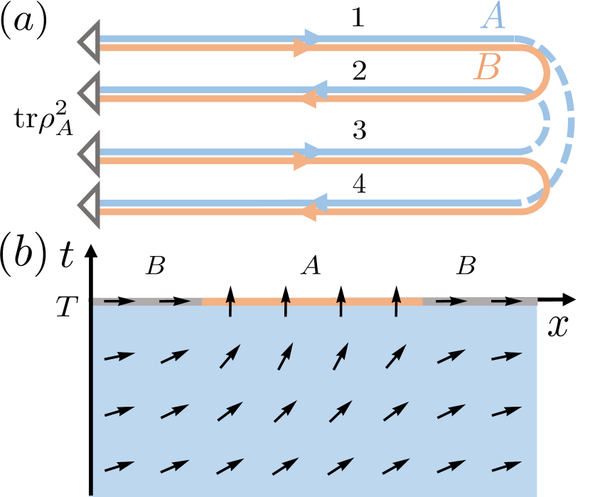
The calculation of entanglement entropy can be mapped to the problem of computing the energy of half-vortex pair that emerges due to the special boundary conditions in the Rényi contour [25]. To illustrate this, we consider the evolution time to be long enough and focus on the boundary at . For subsystem , the twisted boundary conditions connect branches and (see FIG. 2 (a)) which excites the Goldstone mode and effectively imposes a vortex on one boundary region of and a antivortex on the other. On the contrary, for subsystem , the boundary condition favors according to previous analysis. Together with the effective action (10), the problem maps to (infinite copies of) 2D XY models on a half-infinite plane with additional pinning fields creating half-vortex/antivortex on the boundaries. A sketch for this system is shown in FIG. 2 (b). The entanglement entropy (13) is equal to the energy of this half-vortex-antivortex pair with spatial separation , which is known to be [63, 64]; such a critical behavior is consistent with previous numerics [35]. Similarly, the mutual information is equal to (the absolute value of) the interaction energy between two half-vortex pairs, which scales with where is the distance between two subregions.
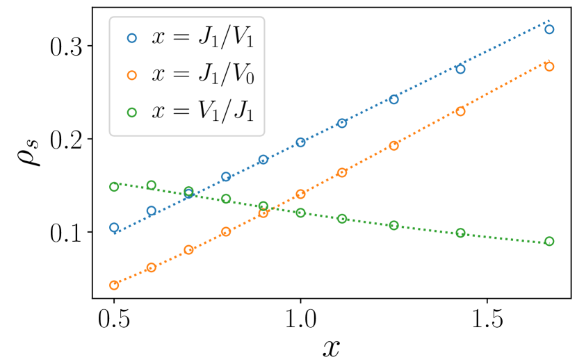
In the large- limit, the XY model is at zero-temperature and we can directly apply the mean-field approximation. The stiffness (or the superfluid density) is given by summing up contributions from different , which gives
| (14) |
Specifically, for large and the result is consistent with the numerical observation in [35]. We further perform numerical simulation to verify that the scaling form (14) holds in a large parameter region with finite and ; the numerical result for the stiffness is shown in Fig. 3 [73].
6 Connections to circuits at finite
The non-unitary random dynamics of free fermion models are also considered in [33, 34, 25] using Gaussian fermionic circuits. In all these works, the steady states exhibit critical phases which have logarithmic entanglement entropy and are interpreted in different approaches. In [33], authors propose a non-linear master equation for squared correlators, which predicts the scaling, consistent with the numerics. In [25], authors argue the replicated random fermionic circuits can be described by an effective sine-Gordon theory. Different from our result, there is only a single Goldstone mode when the system is in the critical phase. This is due to the absence of energy conservation, which couples fermion modes with different frequencies. Similar behavior can also be observed if we consider the Brownian non-Hermitian SYK2 chains, and we leave this discussion in the Appendix C.
7 Discussions
In this work, we study the non-unitary dynamics of the SYK2 chains for both the static model and the Brownian model. In the replicated space, either system shows (copies) of the symmetry, which is broken into by the saddle-point solution. The system then obtains an emergent replica conformal symmetry from the fluctuation of Goldstone modes, leading to the universal scaling of squared correlators. The entanglement entropy of a subsystem can be understood as the energy of a half-vortex pair, which is logarithmic in the subsystem size.
There are a lot of interesting extensions of this work. Firstly, our derivations can be directly applied to the higher dimensional SYK2 lattices with minor modifications. For 2D lattices, the result is an XY model in 3D. Choosing subsystem as a circle with perimeter , the entanglement entropy then corresponds to the energy of a half-vortex ring, which is proportional to . Secondly, we can add interactions to our model. As an example, consider adding a Brownian SYK4 interaction . This leads to an additional self-energy term , which breaks the symmetry explicitly. Consequently, the replicated system becomes gapped, and there is no conformal symmetry anymore. Furthermore, the entanglement entropy corresponds to the energy of a domain wall with length , instead of a vortex pair, leading to the volume law. Finally, it is also interesting to construct models with entanglement transitions. Such a model exists if we introduce two copies of the SYK chain and add non-Hermiticity on the fermion parity operator between two copies. The system shows a transition between a critical phase and an area law phase when there is no interaction. After adding interactions, the system shows a second-order transition between a volume-law phase to an area-law phase. These results will be presented in a separate paper [74].
Acknowledgment. We acknowledge helpful discussions with Ehud Altman. PZ acknowledges support from the Walter Burke Institute for Theoretical Physics at Caltech. SKJ is supported by the Simons Foundation via the It From Qubit Collaboration. CL is supported by the NSF CMMT program under Grants No. DMR-1818533. Use was made of computational facilities purchased with funds from the National Science Foundation (CNS-1725797) and administered by the Center for Scientific Computing (CSC). The CSC is supported by the California NanoSystems Institute and the Materials Research Science and Engineering Center (MRSEC; NSF DMR-1720256) at UC Santa Barbara.
References
- Srednicki [1994] Mark Srednicki. Chaos and quantum thermalization. Phys. Rev. E, 50:888–901, Aug 1994. doi: 10.1103/PhysRevE.50.888.
- Deutsch [1991] J. M. Deutsch. Quantum statistical mechanics in a closed system. Phys. Rev. A, 43:2046–2049, Feb 1991. doi: 10.1103/PhysRevA.43.2046.
- Nandkishore and Huse [2015] Rahul Nandkishore and David A. Huse. Many-body localization and thermalization in quantum statistical mechanics. Annual Review of Condensed Matter Physics, 6(1):15–38, 2015. doi: 10.1146/annurev-conmatphys-031214-014726.
- Alet and Laflorencie [2018] Fabien Alet and Nicolas Laflorencie. Many-body localization: An introduction and selected topics. Comptes Rendus Physique, 19(6):498–525, 2018. doi: 10.1016/j.crhy.2018.03.003.
- Abanin et al. [2017] Dmitry Abanin, Wojciech De Roeck, Wen Wei Ho, and François Huveneers. A rigorous theory of many-body prethermalization for periodically driven and closed quantum systems. Communications in Mathematical Physics, 354(3):809–827, 2017. doi: 10.1007/s00220-017-2930-x.
- Kuwahara et al. [2016] Tomotaka Kuwahara, Takashi Mori, and Keiji Saito. Floquet–magnus theory and generic transient dynamics in periodically driven many-body quantum systems. Annals of Physics, 367:96–124, 2016. doi: 10.1016/j.aop.2016.01.012.
- Banerjee [2018] Subhashish Banerjee. Open quantum systems. Springer, 2018. doi: 10.1007/978-981-13-3182-4.
- Li et al. [2018] Yaodong Li, Xiao Chen, and Matthew P. A. Fisher. Quantum zeno effect and the many-body entanglement transition. Phys. Rev. B, 98:205136, Nov 2018. doi: 10.1103/PhysRevB.98.205136.
- Cao et al. [2019] Xiangyu Cao, Antoine Tilloy, and Andrea De Luca. Entanglement in a fermion chain under continuous monitoring. SciPost Phys., 7:24, 2019. doi: 10.21468/SciPostPhys.7.2.024.
- Li et al. [2019] Yaodong Li, Xiao Chen, and Matthew P. A. Fisher. Measurement-driven entanglement transition in hybrid quantum circuits. Phys. Rev. B, 100:134306, Oct 2019. doi: 10.1103/PhysRevB.100.134306.
- Skinner et al. [2019] Brian Skinner, Jonathan Ruhman, and Adam Nahum. Measurement-induced phase transitions in the dynamics of entanglement. Phys. Rev. X, 9:031009, Jul 2019. doi: 10.1103/PhysRevX.9.031009.
- Chan et al. [2019] Amos Chan, Rahul M. Nandkishore, Michael Pretko, and Graeme Smith. Unitary-projective entanglement dynamics. Phys. Rev. B, 99:224307, Jun 2019. doi: 10.1103/PhysRevB.99.224307.
- Bao et al. [2020] Yimu Bao, Soonwon Choi, and Ehud Altman. Theory of the phase transition in random unitary circuits with measurements. Physical Review B, 101(10), Mar 2020. ISSN 2469-9969. doi: 10.1103/physrevb.101.104301.
- Choi et al. [2020] Soonwon Choi, Yimu Bao, Xiao-Liang Qi, and Ehud Altman. Quantum error correction in scrambling dynamics and measurement-induced phase transition. Physical Review Letters, 125(3), Jul 2020. ISSN 1079-7114. doi: 10.1103/physrevlett.125.030505.
- Gullans and Huse [2020a] Michael J Gullans and David A Huse. Dynamical purification phase transition induced by quantum measurements. Physical Review X, 10(4):041020, 2020a. doi: 10.1103/PhysRevX.10.041020.
- Gullans and Huse [2020b] Michael J. Gullans and David A. Huse. Scalable probes of measurement-induced criticality. Phys. Rev. Lett., 125:070606, Aug 2020b. doi: 10.1103/PhysRevLett.125.070606.
- Jian et al. [2020a] Chao-Ming Jian, Yi-Zhuang You, Romain Vasseur, and Andreas W. W. Ludwig. Measurement-induced criticality in random quantum circuits. Phys. Rev. B, 101:104302, Mar 2020a. doi: 10.1103/PhysRevB.101.104302.
- Zabalo et al. [2020] Aidan Zabalo, Michael J. Gullans, Justin H. Wilson, Sarang Gopalakrishnan, David A. Huse, and J. H. Pixley. Critical properties of the measurement-induced transition in random quantum circuits. Phys. Rev. B, 101:060301, Feb 2020. doi: 10.1103/PhysRevB.101.060301.
- Tang and Zhu [2020] Qicheng Tang and W. Zhu. Measurement-induced phase transition: A case study in the nonintegrable model by density-matrix renormalization group calculations. Phys. Rev. Research, 2:013022, Jan 2020. doi: 10.1103/PhysRevResearch.2.013022.
- Szyniszewski et al. [2019] M. Szyniszewski, A. Romito, and H. Schomerus. Entanglement transition from variable-strength weak measurements. Phys. Rev. B, 100:064204, Aug 2019. doi: 10.1103/PhysRevB.100.064204.
- Zhang et al. [2020a] Lei Zhang, Justin A. Reyes, Stefanos Kourtis, Claudio Chamon, Eduardo R. Mucciolo, and Andrei E. Ruckenstein. Nonuniversal entanglement level statistics in projection-driven quantum circuits. Physical Review B, 101(23), Jun 2020a. ISSN 2469-9969. doi: 10.1103/physrevb.101.235104.
- Goto and Danshita [2020] Shimpei Goto and Ippei Danshita. Measurement-Induced Transitions of the Entanglement Scaling Law in Ultracold Gases with Controllable Dissipation. arXiv e-prints, art. arXiv:2001.03400, January 2020.
- Jian et al. [2021a] Shao-Kai Jian, Zhi-Cheng Yang, Zhen Bi, and Xiao Chen. Yang-lee edge singularity triggered entanglement transition. arXiv preprint arXiv:2101.04115, 2021a.
- Buchhold et al. [2021] M Buchhold, Y Minoguchi, A Altland, and S Diehl. Effective theory for the measurement-induced phase transition of dirac fermions. arXiv preprint arXiv:2102.08381, 2021.
- Bao et al. [2021] Yimu Bao, Soonwon Choi, and Ehud Altman. Symmetry enriched phases of quantum circuits. arXiv preprint arXiv:2102.09164, 2021.
- Sang and Hsieh [2021] Shengqi Sang and Timothy H Hsieh. Measurement-protected quantum phases. Physical Review Research, 3(2):023200, 2021. doi: 10.1103/PhysRevResearch.3.023200.
- Lavasani et al. [2021] Ali Lavasani, Yahya Alavirad, and Maissam Barkeshli. Measurement-induced topological entanglement transitions in symmetric random quantum circuits. Nature Physics, 17(3):342–347, Jan 2021. ISSN 1745-2481. doi: 10.1038/s41567-020-01112-z.
- Ippoliti et al. [2021a] Matteo Ippoliti, Tibor Rakovszky, and Vedika Khemani. Fractal, logarithmic and volume-law entangled non-thermal steady states via spacetime duality. arXiv preprint arXiv:2103.06873, 2021a.
- Lu and Grover [2021] Tsung-Cheng Lu and Tarun Grover. Entanglement transitions via space-time rotation of quantum circuits. arXiv preprint arXiv:2103.06356, 2021.
- Jian et al. [2020b] Chao-Ming Jian, Bela Bauer, Anna Keselman, and Andreas WW Ludwig. Criticality and entanglement in non-unitary quantum circuits and tensor networks of non-interacting fermions. arXiv preprint arXiv:2012.04666, 2020b.
- Ippoliti et al. [2021b] Matteo Ippoliti, Michael J. Gullans, Sarang Gopalakrishnan, David A. Huse, and Vedika Khemani. Entanglement phase transitions in measurement-only dynamics. Physical Review X, 11(1), Feb 2021b. ISSN 2160-3308. doi: 10.1103/physrevx.11.011030.
- Carollo and Alba [2021] Federico Carollo and Vincenzo Alba. Emergent dissipative quasi-particle picture in noninteracting markovian open quantum systems. arXiv preprint arXiv:2106.11997, 2021.
- Chen et al. [2020a] Xiao Chen, Yaodong Li, Matthew P. A. Fisher, and Andrew Lucas. Emergent conformal symmetry in nonunitary random dynamics of free fermions. Physical Review Research, 2(3):033017, Jul 2020a. ISSN 2643-1564. doi: 10.1103/physrevresearch.2.033017.
- Alberton et al. [2021] Ori Alberton, Michael Buchhold, and Sebastian Diehl. Entanglement transition in a monitored free-fermion chain: From extended criticality to area law. Physical Review Letters, 126(17):170602, 2021. doi: 10.1103/PhysRevLett.126.170602.
- Liu et al. [2021] Chunxiao Liu, Pengfei Zhang, and Xiao Chen. Non-unitary dynamics of sachdev-ye-kitaev chain. SciPost Physics, 10(2):Art–No, 2021. doi: 10.21468/SciPostPhys.10.2.048.
- Kitaev [2015] Alexei Kitaev. A simple model of quantum holography, talk given at the kitp program: entanglement in strongly-correlated quantum matter. talk given at the KITP Program: entanglement in strongly-correlated quantum matter, 2015.
- Maldacena and Stanford [2016] Juan Maldacena and Douglas Stanford. Remarks on the sachdev-ye-kitaev model. Phys. Rev. D, 94:106002, Nov 2016. doi: 10.1103/PhysRevD.94.106002.
- Sachdev and Ye [1993] Subir Sachdev and Jinwu Ye. Gapless spin-fluid ground state in a random quantum heisenberg magnet. Phys. Rev. Lett., 70:3339–3342, May 1993. doi: 10.1103/PhysRevLett.70.3339.
- Liu et al. [2018] Chunxiao Liu, Xiao Chen, and Leon Balents. Quantum entanglement of the sachdev-ye-kitaev models. Phys. Rev. B, 97:245126, Jun 2018. doi: 10.1103/PhysRevB.97.245126.
- Gu et al. [2017a] Yingfei Gu, Andrew Lucas, and Xiao-Liang Qi. Spread of entanglement in a Sachdev-Ye-Kitaev chain. Journal of High Energy Physics, 2017(9):120, September 2017a. doi: 10.1007/JHEP09(2017)120.
- Huang and Gu [2019] Yichen Huang and Yingfei Gu. Eigenstate entanglement in the sachdev-ye-kitaev model. Phys. Rev. D, 100:041901, Aug 2019. doi: 10.1103/PhysRevD.100.041901.
- Zhang et al. [2020b] Pengfei Zhang, Chunxiao Liu, and Xiao Chen. Subsystem Rényi Entropy of Thermal Ensembles for SYK-like models. SciPost Phys., 8:94, 2020b. doi: 10.21468/SciPostPhys.8.6.094.
- Haldar et al. [2020] Arijit Haldar, Surajit Bera, and Sumilan Banerjee. Rényi entanglement entropy of fermi and non-fermi liquids: Sachdev-ye-kitaev model and dynamical mean field theories. Phys. Rev. Research, 2:033505, Sep 2020. doi: 10.1103/PhysRevResearch.2.033505.
- [44] Pengfei Zhang. Entanglement entropy and its quench dynamics for pure states of the sachdev-ye-kitaev model. Journal of High Energy Physics, (6):143. doi: 10.1007/JHEP06(2020)143.
- Chen et al. [2020b] Yiming Chen, Xiao-Liang Qi, and Pengfei Zhang. Replica wormhole and information retrieval in the syk model coupled to majorana chains. Journal of High Energy Physics, 2020(6):121, 2020b. doi: 10.1007/JHEP06(2020)121.
- Shao-Kai and Swingle [2021] Jian Shao-Kai and Brian Swingle. Note on entropy dynamics in the brownian syk model. Journal of High Energy Physics, 2021(3), 2021. doi: 10.1007/JHEP03(2021)042.
- Gu et al. [2017b] Yingfei Gu, Xiao-Liang Qi, and Douglas Stanford. Local criticality, diffusion and chaos in generalized Sachdev-Ye-Kitaev models. Journal of High Energy Physics, 2017(5):125, May 2017b. doi: 10.1007/JHEP05(2017)125.
- Davison et al. [2017] Richard A. Davison, Wenbo Fu, Antoine Georges, Yingfei Gu, Kristan Jensen, and Subir Sachdev. Thermoelectric transport in disordered metals without quasiparticles: The sachdev-ye-kitaev models and holography. Phys. Rev. B, 95:155131, Apr 2017. doi: 10.1103/PhysRevB.95.155131.
- Chen et al. [2017] Xin Chen, Ruihua Fan, Yiming Chen, Hui Zhai, and Pengfei Zhang. Competition between chaotic and nonchaotic phases in a quadratically coupled sachdev-ye-kitaev model. Phys. Rev. Lett., 119:207603, Nov 2017. doi: 10.1103/PhysRevLett.119.207603.
- Song et al. [2017] Xue-Yang Song, Chao-Ming Jian, and Leon Balents. Strongly correlated metal built from sachdev-ye-kitaev models. Phys. Rev. Lett., 119:216601, Nov 2017. doi: 10.1103/PhysRevLett.119.216601.
- Zhang [2017] Pengfei Zhang. Dispersive sachdev-ye-kitaev model: Band structure and quantum chaos. Phys. Rev. B, 96:205138, Nov 2017. doi: 10.1103/PhysRevB.96.205138.
- Jian et al. [2017] Chao-Ming Jian, Zhen Bi, and Cenke Xu. Model for continuous thermal metal to insulator transition. Phys. Rev. B, 96:115122, Sep 2017. doi: 10.1103/PhysRevB.96.115122.
- Chen et al. [2017] Yiming Chen, Hui Zhai, and Pengfei Zhang. Tunable quantum chaos in the Sachdev-Ye-Kitaev model coupled to a thermal bath. Journal of High Energy Physics, 2017(7):150, July 2017. doi: 10.1007/JHEP07(2017)150.
- Saad et al. [2018] Phil Saad, Stephen H Shenker, and Douglas Stanford. A semiclassical ramp in syk and in gravity. arXiv preprint arXiv:1806.06840, 2018.
- Sünderhauf et al. [2019] Christoph Sünderhauf, Lorenzo Piroli, Xiao-Liang Qi, Norbert Schuch, and J. Ignacio Cirac. Quantum chaos in the Brownian SYK model with large finite N : OTOCs and tripartite information. Journal of High Energy Physics, 2019(11):38, November 2019. doi: 10.1007/JHEP11(2019)038.
- Lashkari et al. [2013] Nima Lashkari, Douglas Stanford, Matthew Hastings, Tobias Osborne, and Patrick Hayden. Towards the fast scrambling conjecture. Journal of High Energy Physics, 2013(4), Apr 2013. ISSN 1029-8479. doi: 10.1007/jhep04(2013)022.
- Zhou and Chen [2019] Tianci Zhou and Xiao Chen. Operator dynamics in a brownian quantum circuit. Physical Review E, 99(5), May 2019. ISSN 2470-0053. doi: 10.1103/physreve.99.052212.
- Xu and Swingle [2019] Shenglong Xu and Brian Swingle. Locality, quantum fluctuations, and scrambling. Physical Review X, 9(3), Sep 2019. ISSN 2160-3308. doi: 10.1103/physrevx.9.031048.
- Chen and Zhou [2019] Xiao Chen and Tianci Zhou. Quantum chaos dynamics in long-range power law interaction systems. Physical Review B, 100(6), Aug 2019. ISSN 2469-9969. doi: 10.1103/physrevb.100.064305.
- Lucas [2019] Andrew Lucas. Quantum many-body dynamics on the star graph. arXiv e-prints, art. arXiv:1903.01468, March 2019.
- Piroli et al. [2020] Lorenzo Piroli, Christoph Sünderhauf, and Xiao-Liang Qi. A random unitary circuit model for black hole evaporation. Journal of High Energy Physics, 2020(4), Apr 2020. ISSN 1029-8479. doi: 10.1007/jhep04(2020)063.
- fn [5] Different from previous studies for the interplay between Goldstone modes and entanglement entropy in [75, 76] for systems with conventional symmetry breaking, here the conformal symmetry only appears upon introducing replicas.
- Pethick and Smith [2008] C.J. Pethick and H. Smith. Bose–Einstein Condensation in Dilute Gases. Cambridge University Press, 2008. doi: 10.1017/CBO9780511802850.
- Zhai [2021] Hui Zhai. Ultracold Atomic Physics. Cambridge University Press, 2021. doi: 10.1017/9781108595216.
- García-García et al. [2021] Antonio M García-García, Yiyang Jia, Dario Rosa, and Jacobus JM Verbaarschot. Replica symmetry breaking and phase transitions in a pt symmetric sachdev-ye-kitaev model. arXiv preprint arXiv:2102.06630, 2021.
- Kitaev and Suh [2018] Alexei Kitaev and S. Josephine Suh. The soft mode in the Sachdev-Ye-Kitaev model and its gravity dual. Journal of High Energy Physics, 2018(5):183, May 2018. doi: 10.1007/JHEP05(2018)183.
- Gu et al. [2020] Yingfei Gu, Alexei Kitaev, Subir Sachdev, and Grigory Tarnopolsky. Notes on the complex Sachdev-Ye-Kitaev model. Journal of High Energy Physics, 2020(2):157, February 2020. doi: 10.1007/JHEP02(2020)157.
- Winer et al. [2020] Michael Winer, Shao-Kai Jian, and Brian Swingle. Exponential ramp in the quadratic sachdev-ye-kitaev model. Physical Review Letters, 125(25):250602, 2020. doi: 10.1103/PhysRevLett.125.250602.
- fn [1] Note that at the level of the Schwinger-Dyson equation, the phase introduced here is unnecessary. The choice is to make the symmetry not broken by the saddle-point solution.
- fn [6] We verify this numerically within the disorder replica diagonal assumption by solving the Schwinger-Dyson equation at large but finite .
- fn [2] The block diagonal form is verified numerically.
- fn [3] This is similar to the Brownian SYK2 chain model.
- fn [4] In the numerics, we take the initial state to be the maximally entangled state between Majorana fermions with even and odd indices where . The numerical details have been explained in previous works [35].
- Jian et al. [2021b] Shao-Kai Jian, Chunxiao Liu, Xiao Chen, Brian Swingle, and Pengfei Zhang. Measurement-induced phase transition in the monitored sachdev-ye-kitaev model. Physical Review Letters, 127(14):140601, 2021b. doi: 10.1103/PhysRevLett.127.140601.
- Metlitski and Grover [2011] Max A Metlitski and Tarun Grover. Entanglement entropy of systems with spontaneously broken continuous symmetry. arXiv preprint arXiv:1112.5166, 2011.
- Alba [2021] Vincenzo Alba. Entanglement gap, corners, and symmetry breaking. SciPost Phys., 10:56, 2021. doi: 10.21468/SciPostPhys.10.3.056.
Appendix A The path-integral representation of the replicated system
As explained in the main text, we focus on the path-integral representation of the replicated system. The time evolution of a density matrix is
| (15) |
and it does not preserve the normalization. To evaluate using path integral, one needs two contours similar to the Keldysh contour. Denoted by and for forward and backward evolution, the action on these two contours schematically is
where denotes two contours, and the superscript for Majorana species on each site is suppressed. After introducing two replicas, we aim to compute
| (17) |
This basically doubles the action on the Keldysh contour. Namely, it requires four contours denoted by 1, 2, 3, 4. The effective action on these four contours after integrating out disorder is
| (18) | |||||
where and are the bilocal fields with time arguments and omitted, which characterize the two point function of Majarana fermions or the corresponding seld-energy at and contours. As a result, the saddle point equation is
| (19) | |||||
| (20) |
Appendix B The derivation of the effective action
The effective action is given by expanding the action (18) or (48) around the saddle-point solution. In this section, we give a detailed derivation for the effective actions.
B.1 The effective action of the static model
We consider the saddle point fluctuations,
| (21) |
and similar for , where we have used the convention for Fourier transformation. The trace log term in (18) gives rise to [as the first line in (18) does not depend on lattice site, we suppress lattice index until we move on to evaluate the second line in (18)]
| (22) |
where we have defined for conciseness. We will be interested in the correlation between , and , , so we focus on these correlation functions. Assuming the symmetry , we can bring the kernel into
| (27) |
where we have defined and .
If one notices the coupling term in (18), then it is a straightforward task to integrate out field, and the resultant action reads
| (33) |
where . We restore the lattice index by going to the momentum space using with the number of sites.
The second line in (18) is simple, and leads to
| (38) |
So the effective action is given by the sum of (B.1) and (38).
The fields and are related to a Goldstone mode. More precisely, is the Goldstone mode, so they are gapless at zero frequency and momentum. Expanding the effetive action near zero frequency and keeping the leading term, it reads
| (41) | |||
| (44) |
where we make the symmetrization and antisymmetrization of the fields , like the conventional Kelydsh rotation. And remember , . Only keeping the part and expand each element to the leading order in small and , we get the effective action presented in the main text.
B.2 Relation to the entanglement entropy
Here we explain the boundary condition for when computing the entanglement entropy. As discussed in the main text, the entanglement entropy corresponds to
| (45) |
In other words, for sites in the subsystem , the boundary condition connects the forward and the backward evolution in the same replica which favors and , while for sites in the subsystem , the boundary condition connects the forward and the backward evolution in different replicas which favors and . This directly corresponds to the excitation of Goldstone modes. More explicitly, if we work out the low-energy manifold
| (46) |
Then in subsystem, the boundary condition favors or . Computing the entropy corresponds to the calculation of the energy of two half-vortexes with opposite charge.
Appendix C The Brownian non-Hermitian SYK2 chains
We can also generalize our SYK2 chain to the Brownian case. Now, we treat , , , as time-dependent variables with
| (47) | ||||
Since the Hamiltonian is time-dependent, and we keep the time-ordering in (15) and (17) implicit. Following similar steps, the result reads
| (48) | |||||
Here we have ommited the time arguments for bilocal fields as in the static case. The main difference compared to the static case is the appearance of the additional due to the lack of correlation in the time direction. This gives
| (49) | |||||
| (50) |
Different from the static case, now there is only a single symmetry, given by the transformation with . The saddle-point solution takes a simpler form
| (51) |
Here is the quasi-particle decay rate. Similar to the static case, the saddle-point solution also breaks the symmetry down to , leading to a single Goldstone mode.
Now we consider saddle-point fluctuations,
| (52) |
We first evaluate the term and then the interaction terms. Expanding the term into second order, we arrive at
| (53) |
where , and we have used the Fourier transform . In evaluating the kernel, we have used the symmetry of bilocal field , so there are four independent diagonal fields and six independent off-diagonal fields. The full kernel implies that (a) off-diagonal fields decouple from diagonal field and (b) four out of six independent off-diagonal fields have nontrivial interactions. We denote these four nontrivial off-diagonal fields to be , and the corresponding kernel reads
| (58) |
It is easy to check that the kernel has two zero modes, and we can make redefinition of the fields
| (63) |
such that the last two fields are zero modes and the quadratic action for the first two fields are (we use to denote the first two fields in the following)
| (66) |
Now we are ready to integrate out fields. For the two zero modes, because they couple linearly to fields in the action (48), integrating them out leads to two constraints.
| (67) |
For notational simplicity, we introduce another fields
| (68) |
In terms of these field of interest , , the quadratic action reads
| (69) |
where we restore the space index and make Fourier transform to momentum space in the second line, , is the number of the site of the chain. And we also define , , and one should distinguish it from the case of regular SYK2 model. It is then straightforward to integrate out field to have
| (72) |
Expanding each element to the leading order in small and , we get
| (73) |
In terms of the coset space variable , this becomes the effective action of a single Goldstone mode
| (74) |
which takes a similar form as the static case due to the time-reversal symmetry. Consequently, the universal scaling of the squared correlators still applies and can be extracted from (74) to obtain
| (75) |
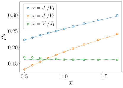
Such a scaling is again verified numerically; the numerical value of the stiffness is shown in Fig. 4.
Appendix D Discussions on special limits of the model
As mentioned in the main text, in special limits, the symmetry of the system can be larger and additional Goldstone modes appear. In this section, we give a detailed discussions on these cases. We take the static case as an example, and finally comment on the Brownian case.
For the saddle-point equation (19), we consider:
-
1.
In special cases the symmetry of the equation can be larger than (for each frequency ). For example, when we have purely Hermitian evolution with , we can define . The self-consistent equation then reads
(76) The equation now becomes symmetric: with arbitrary matrices . The effective action now leads to diffusive behavior
(77) where we have dropped non-universal coefficients.
-
2.
There is additional symmetry between the forward and the backward evolution if and . The reason is that if we consider two evolutions and neglect their boundary conditions
(78) If we define , we find with unchanged. Consequently, There is an additional Goldstone mode with momentum . The mode appears at and . Explicitly, we have
(79) -
3.
Similar modes exists when we instead have and . The idea is again to perform the transformation . The self-energy becomes:
(80) Back to the evolution operator language, this corresponds to the self-consistent equation of
(81) Here we neglect boundary conditions. Now if we perform a momentum shift by for contours, then the path-integral show symmetry, and again we have modes on and . Note that compared to the previous case, the frequency for the modes are different. This leads to
(82) -
4.
The purely imaginary evolution with is also special. On the one hand, both contours are symmetric and there should be symmetry. However, in this case we have and there should be no symmetry breaking and thus no Goldstone modes. Calculation gives
(83)
For the Brownian model, similar analysis shows for and , there is a similar Goldstone mode at and . However, when and , the mode does not appear due to the lack of correlation in the time domain. Furthermore, different from the static model, is non-trivial even under the purely imaginary evolution. Consequently, the result is the same as the general case, as mentioned in the main text.