Energy-independent optical ${}^{1}S_{0}NN$ potential
from Marchenko equation

Abstract

We present a new algebraic method for solving the inverse problem of quantum scattering theory based on the Marchenko theory. We applied a triangular wave set for the Marchenko equation kernel expansion in a separable form. The separable form allows a reduction of the Marchenko equation to a system of linear equations. For the zero orbital angular momentum, a linear expression of the kernel expansion coefficients is obtained in terms of the Fourier series coefficients of a function depending on the momentum $q$ and determined by the scattering data in the finite range of $q$. It is shown that a Fourier series on a finite momentum range ($0<q<\pi/h$) of a $q(1-S)$ function ($S$ is the scattering matrix) defines the potential function of the corresponding radial Schrödinger equation with $h$-step accuracy. A numerical algorithm is developed for the reconstruction of the optical potential from scattering data. The developed procedure is applied to analyze the ${}^{1}S_{0}NN$ data up to 3 GeV. It is shown that these data are described by optical energy-independent partial potential.

I INTRODUCTION

The inverse problem of quantum scattering is essential for various physical applications such as the internuclear potential extraction from scattering data and similar problems. The main approaches to solving the problem are Marchenko, Krein, and Gelfand-Levitan theories Gelfand ; Agranovich1963 ; Marchenko1977 ; Krein1955 ; Levitan1984 ; Newton ; Chadan . The ill-posedness of the inverse problem complicates its numerical solution. So far, the development of robust methods for solving the problem remains a fundamental challenge for applications. This paper considers a new algebraic method for solving the inverse problem of quantum scattering theory. We derive the method from the Marchenko theory. To this end, we propose a novel numerical solution of the Marchenko equation based on the integral kernel approximation as a separable series in the triangular and rectangular wave sets. Then we show that the series coefficients may be calculated directly from the scattering data on the finite segment of the momentum axis. We offer an exact relationship between the potential function accuracy and the range of known scattering data.

The concept of optical potential (OP) is a useful tool in many branches of nuclear physics. There are a number of microscopically derived Timofeyuk2020 ; Burrows2020 ; Tung2020 ; Dinmore2019 ; Vorabbi2018 ; Wang2018 ; Atkinson2018 ; Yahya2018 ; Lee2018 ; Vorabbi2017 ; Fernandez-Soler2017 ; Guo2017 ; Rotureau2017 ; Vorabbi2016 as well as phenomenological Vorabbi2018 ; Guo2017 ; Kobos1985 ; Hlophe2013 ; Khokhlov2006 ; Xu2016 ; Ivanov2016 ; Quinonez2020 ; Jaghoub2018 ; Titus2016 optical potentials used for description of nuclei and nuclear reactions. Nucleon-nucleon potentials are used as an input for (semi)microscopic descriptions of nuclei and nuclear reactions Timofeyuk2020 ; Burrows2020 ; Vorabbi2018 ; Vorabbi2017 ; Guo2017 ; Xu2016 ; Vorabbi2016 . We analyzed the Marchenko theory Agranovich1963 ; Marchenko1977 and found that it is applicable not only to unitary $S$-matrices but also to non-unitary $S$-matrices describing absorption. That is, the Marchenko equation and our algebraic form of the Marchenko equation allow us to reconstruct local and energy-independent OP from an absorbing $S$-matrix and characteristics of corresponding bound states. We applied the developed formalism to analyze the ${}^{1}S_{0}NN$ data up to 3 GeV and showed that these data are described by energy-independent optical partial potential. Our results contradict conclusions of Fernandez-Soler2017 where they state that ”… the optical potential with a repulsive core exhibits a strong energy dependence whereas the optical potential with the structural core is characterized by a rather adiabatic energy dependence …” On the contrary, we reconstructed from the scattering data local and energy-independent $NN$ soft core OP.

II Marchenko equation in an algebraic form

We write the radial Schrödinger equation in the form:

$$\left(\frac{d^{2}}{dr^{2}}-\frac{l(l+1)}{r^{2}}-V(r)+q^{2}\right)\psi(r,q)=0.$$ (1)

Initial data for the Marchenko method [1] are:

$$\left\{S(q),(0<q<\infty),\tilde{q}_{j},M_{j},j=1,\ldots,n\right\},$$ (2)

where $S(q)=e^{2\imath\delta(q)}$ is a scattering matrix dependent on the momentum $q$. The $S$-matrix defines asymptotic behavior at $r\rightarrow+\infty$ of regular at $r=0$ solutions of Eq. (1) for $q\geq 0;\ \tilde{q}_{j}^{2}=E_{j}\leq 0,E_{j}$ is $j$-th bound state energy ($-\imath\tilde{q}_{j}\geq 0$); $M_{j}$ is $j$-th bound state asymptotic constant. The Marchenko equation is a Fredholm integral equation of the second kind:

$$F(x,y)+L(x,y)+\int_{x}^{+\infty}L(x,t)F(t,y)dt=0$$ (3)

We write the kernel function as

$$F(x,y)=\frac{1}{2\pi}\int_{-\infty}^{+\infty}h_{l}^{+}(qx)[1-S(q)]h_{l}^{+}(qy)dq\\ +\sum_{j=1}^{n_{b}}h_{l}^{+}\left(\tilde{q}_{j}x\right)M_{j}^{2}h_{l}^{+}\left(\tilde{q}_{j}y\right)\\ =\frac{1}{2\pi}\int_{-\infty}^{+\infty}h_{l}^{+}(qx)Y(q)h_{l}^{+}(qy)dq$$ (4)

where

$$Y(q)=\left[1-S(q)-i\sum_{j=1}^{n_{b}}M_{j}^{2}\left(q-\tilde{q}_{j}\right)^{-1}\right]$$ (5)

Solution of Eq. (3) gives the potential of Eq. (1):

$$V(r)=-2\frac{dL(r,r)}{dr}$$ (6)

There are many computational approaches for the solution of Fredholm integral equations of the second kind. Many of the methods use an equation kernel’s series expansion eprint7 ; eprint8 ; eprint9 ; eprint10 ; eprint11 ; eprint12 ; eprint13 ; eprint14 . We also use this technique. Assuming the finite range $R$ of the bounded potential function, we approximate the kernel function as

$$F(x,y)\approx\sum_{k,j=0}^{N}\Delta_{k}(x)F_{k,j}\Delta_{j}(y)$$ (7)

where $F_{k,j}\equiv F(kh,jh)$, and the basis functions are

$$\left.\begin{array}[]{l}\Delta_{0}(x)=\left\{\begin{array}[]{lll}0&\text{ for }&|x|>h,\\ 1+x/h&\text{ for }&-h\leq x\leq 0,\\ 1-x/h&\text{ for }&0<x\leq h;\end{array}\right.\\ \Delta_{n}(x)=\Delta_{0}(x-hn)\end{array}\right\}$$ (8)

where $h$ is some step, and $R=Nh$. Decreasing the step $h$, one can approach the kernel arbitrarily close at all points. As a result, the kernel is presented in a separable form. We solve Eq. (3) substituting

$$L(x,y)\approx\sum_{j=0}^{N}P_{j}(x)\Delta_{j}(y)$$ (9)

Substitution of Eqs. (7) and (9) into Eq. (3), and taking into account the linear independence of the basis functions, gives

$$\sum_{m=0}^{N}\left(\delta_{j\,m}+\sum_{n=0}^{N}\left[\int_{x}^{\infty}\Delta_{m}(t)\Delta_{n}(t)dt\right]F_{n,j}\right)P_{m}(x)=-\sum_{k=0}^{N}\Delta_{k}(x)F_{k,j}$$ (10)

We need values of $P_{k}(hp)\equiv P_{p,k}$ $(p,k=0,..,N)$. In this case integrals in Eq. (10) may be calculated

$$\zeta_{n\,m\,p}=\int_{ph}^{\infty}\Delta_{m}(t)\Delta_{n}(t)dt=\frac{h}{6}\left(2\delta_{n\,n}\left(\delta_{n\,p}+2\eta_{n\geq p+1}\right)+\delta_{n\,(m-1)}\eta_{n\geq p}+\delta_{n\,(m+1)}\eta_{m\geq p}\right)$$ (11)

Here, along with the Kronecker symbols $\delta_{k\,p}$, symbols $\eta_{a}$ are introduced, which are equal to one if the logical expression $a$ is true, and are equal to zero otherwise. Considering also that $\Delta_{k}(hp)\equiv\delta_{k\,p}$, we finally get a system of equations

$$\sum_{m=0}^{N}\left(\delta_{j\,m}+\sum_{n=0}^{N}\zeta_{n\,m\,p}F_{n,j}\right)P_{pm}=-F_{p,j}$$ (12)

for each $j,p=0,..,N$. Solution of Eq. (12) gives $P_{k}(hp)\equiv P_{p,k}$. Potential values at points $r=hp$ $(p=0,..,N)$ are determined from Eq. (6) by some finite difference formula.

Next, we consider the case $l=0$, for which $h_{l}^{+}(qx)=e^{\imath qx}$ and

$$F(x,y)=F(x+y)=\frac{1}{2\pi}\int_{-\infty}^{+\infty}e^{\imath q(x+y)}Y(q)dq.$$ (13)

We approximate the kernel as follows:

$$F(x,y)=F(x+y)\approx\sum_{k=-2N}^{2N}F_{0,k}H_{k}(x+y)$$ (14)

where $F_{0,k}\equiv F(kh)$ as in Eq. (7) for $l=0$, and the used basis set is

$$\left.\begin{array}[]{l}H_{0}(x)=\left\{\begin{array}[]{lll}0&\text{ for }&x<0,\\ 1&\text{ for }&0\leq x\leq h,\\ 0&\text{ for }&x>h,\end{array}\right.\\ H_{n}(x)=H_{0}(x-hn).\end{array}\right\}$$ (15)

The Fourier transform of the basis set Eq. (15) is

$$\tilde{\mathrm{H}}_{k}(q)=\int_{-\infty}^{\infty}\mathrm{H}_{k}(x)e^{-\imath qx}dx=\frac{\imath\left(e^{-iqh}-1\right)}{q}e^{-\imath qhk}.$$ (16)

The function $Y(q)$ may be presented as

$$Y(q)=\sum_{k=-2N}^{2N}F_{0,k}\tilde{\mathrm{H}}_{k}(q)=\sum_{k=-2N}^{2N}F_{0,k}\frac{\imath\left(e^{-\imath qh}-1\right)}{q}e^{-\imath qhk}.$$ (17)

The last relationship may be rearranged

$$qY(q)=\imath\sum_{k=-2N}^{2N}F_{0,k}\left(e^{-\imath qh}-1\right)e^{-\imath qhk}\\ =i\sum_{k=-2N+1}^{2N}\left(F_{0,k-1}-F_{0,k}\right)e^{-\imath qhk}+\imath\left(-F_{0,-2N}\right)e^{\imath qh2N}+\imath\left(F_{0,2N}\right)e^{-\imath qh(2N+1)}.$$ (18)

Thus, the left side of the expression is represented as a Fourier series on the interval $-\pi/h\leq q\leq\pi/h$. Taking into account that $Y(-q)=Y^{*}(q)$, we get

$$\left.\begin{array}[]{l}-F_{0,-2N}=\frac{h}{\pi}\int_{0}^{\pi/h}\text{Im}\left(Y(q)e^{-\imath qh2N}\right)qdq;\\ \\ F_{0,k-1}-F_{0,k}=\frac{h}{\pi}\int_{0}^{\pi/h}\text{Im}\left(Y(q)e^{\imath qhk}\right)qdq\text{ for }k=-2N+1,\ldots,2N-1;\\ \\ F_{0,2N}=\frac{h}{\pi}\int_{0}^{\pi/h}\text{Im}\left(Y(q)e^{\imath qh(2N+1)}\right)qdq.\end{array}\right\}$$ (19)

The system (19) is solved recursively from $F_{0,2N}$. Thus, the range of known scattering data defines the step value $h$ and, therefore, the inversion accuracy. Calculation results for the potential function $V(r)=-3\exp(-3r/2)$ are presented in Figs. 1, 2, where $h=0.04$, $R=4$. $S$-matrix was calculated at points shown in Fig. 1 up to $q=8$. The $S$-matrix was interpolated by a quadratic spline in the range $0<q<8$. For $q>8$ the $S$-matrix was approximated as asymptotic $S(q)\approx\exp(-2iA/q)$ for $q>8$, where $A$ was calculated at $q=8$.

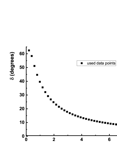
Figure 1: Data used to reconstruct $V(r)=V_{0}\exp(-ar)$, where $V_{0}=-3\ fm^{-2}=-124.5\ MeV$, $a=1.5\ fm^{-1}$. Units correspond to the $NN$ system.

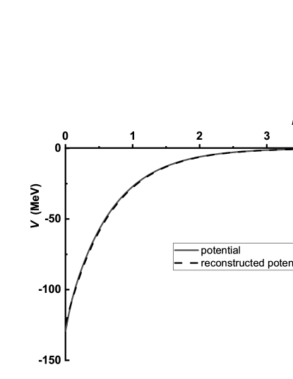
Figure 2: Initial and reconstructed potentials: $V(r)=V_{0}\exp(-ar)$, where $V_{0}=-3\ fm^{-2}=-124.5\ MeV$, $a=1.5\ fm^{-1}$. Units correspond to the $NN$ system.

III Energy-independent optical ${}^{1}S_{0}NN$ potential

Realistic potentials derived unambiguously from inverse theories should describe scattering data from zero to infinite energy. It seems that it is only possible if the available scattering data approach the asymptotic region below the relativistic region. It is unnecessary because relativistic two-particle potential models may be presented in the non-relativistic form Keister1991 . Another problem is the presence of closed channels whose characteristics are not known. It is usually assumed (for example, for an $NN$ system) that below the inelasticity threshold, effects of closed channels can be neglected, and a real $NN$ potential may describe the interaction of nucleons. This assumption is a consequence of the ingrained misconception that a complex potential corresponds to a non-unitary matrix. One can only assert that the $S$-matrix is unitary for a real potential.

We have carefully analyzed the Marchenko theory Agranovich1963 ; Marchenko1977 and found that it applies not only to unitary $S$-matrices but also to non-unitary $S$-matrices describing absorption. That is, the Marchenko theory Eqs. (1-6) and our algebraic form of the Marchenko equation Eqs. (7-18) allow to reconstruct local, and energy-independent OP from an absorbing $S$-matrix and corresponding bound states’ characteristics. We present an absorptive single partial channel $S$-matrix on the $q$-axis as

$$S(q)=\left\{\begin{array}[]{lll}S_{u}(q)+S_{n}(q)&\text{ for }&q>0,\\ S^{+}_{u}(-q)-S^{+}_{n}(-q)&\text{ for }&q<0,\end{array}\right.$$ (20)

where superscript $+$ means hermitian conjugation. For $q>0$ we define

$$S_{u}(q)=e^{2\imath\delta(q)},\\ S_{n}(q)=-\sin^{2}(\rho(q))e^{2\imath\delta(q)},$$ (21)

where $\delta(q)$ and $\rho(q)$ are phase shift and inelastisity parameter correspondingly. In this case we have instead of Eqs. (19) the following system

$$\left.\begin{array}[]{l}-F_{0,-2N}=\frac{h}{\pi}\int_{0}^{\pi/h}q\left[\text{Im}\left(Y_{u}(q)e^{-\imath qh2N}\right)-\imath\text{Re}\left(S_{n}(q)e^{-\imath qh2N}\right)\right]dq;\\ \\ F_{0,k-1}-F_{0,k}=\frac{h}{\pi}\int_{0}^{\pi/h}q\left[\text{Im}\left(Y_{u}(q)e^{\imath qhk}\right)-\imath\text{Re}\left(S_{n}(q)e^{\imath qhk}\right)\right]dq\text{ for }k=-2N+1,\ldots,2N-1;\\ \\ F_{0,2N}=\frac{h}{\pi}\int_{0}^{\pi/h}q\left[\text{Im}\left(Y_{u}(q)e^{\imath qh(2N+1)}\right)-\imath\text{Re}\left(S_{n}(q)e^{\imath qh(2N+1)}\right)\right]dq,\end{array}\right\}$$ (22)

where

$$Y_{u}(q)=\left[1-S_{u}(q)-i\sum_{j=1}^{n_{b}}M_{j}^{2}\left(q-\tilde{q}_{j}\right)^{-1}\right].$$ (23)

IV Results and Conclusions

We applied the developed formalism to analyze the ${}^{1}S_{0}$ $NN$ data. As input data for the reconstruction, we used modern phase shift analysis data (single-energy solutions) up to 3 GeV DataScat ; cite . We smoothed phase shift and inelasticity parameter data for $q>3$ fm^-1 by the following functions:

$$\delta(q)\sim-54.56822/q^{3}+57.55296/q^{2}-15.36687/q,\\ \rho(q)\sim 101.89881/q^{3}-80.13493/q^{2}+15.88984/q,$$ (24)

where we fitted the coefficients by the least-squares method. Asymptotics (24) were used to calculate coefficients of Eqs. (19) with $h=0.0125$ fm corresponding to $q_{max}\approx 251.3$ fm^-1.

Results of our calculations show that these data are described by energy-independent optical partial potential (Figs. 3,4).

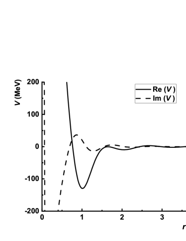
Figure 3: Data used to reconstruct ${}^{1}S_{0}NN$ potential.

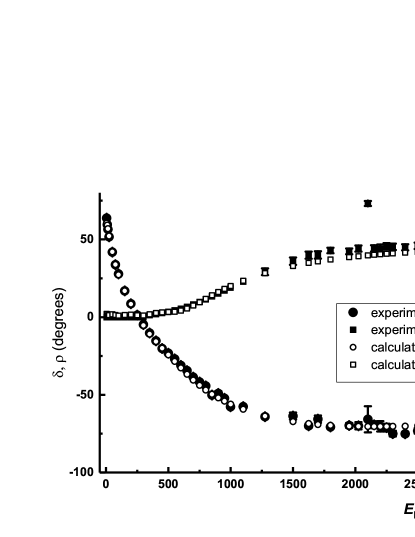
Figure 4: Reconstructed ${}^{1}S_{0}NN$ potential.

Thus, we presented a solution of the quantum scattering inverse problem for the zero orbital angular momentum, the algorithm of which is as follows. We set the step value $h$, which determines a required accuracy of the potential. From the scattering data, we determine $F_{0,k}$ from Eqs. (19) for unitary $S$-matrix or from Eqs. (22) for non-unitary $S$-matrix. Solution of Eqs. (12) gives values of $P_{k}(hp)$ ($p=0,..,N$). Further, the values of the potential function (6) are determined by some finite difference formula. Expressions (7-14) give a method for the Marchenko equation’s numerical solution for an arbitrary orbital angular momentum $l$, and may be generalized for a case of coupled channels.

Our results contradict conclusions of Fernandez-Soler2017 claiming that an OP with a repulsive core exhibits a strong energy dependence. On the contrary, we reconstructed local and energy-independent $NN$ soft core OP with $Re(V(0))\approx 14\ GeV$ and $Im(V(0))\approx 19\ GeV$ .

It may be that some local OPs lead to unsatisfactory description of nuclear reactions Titus2016 ($(d,p)$ transfer reactions). Our approach assumes inverse scattering reconstruction of local and energy-independent OP describing all two-particle scattering data (including high energy asymptotics) and bound states. Such OPs have not been used in nuclear calculations, though they may give an adequate description of the off-shell behaviour of the nucleon-nucleon interaction.

The reconstructed $1S0$ $NN$ optical potential may be requested from the author in the Fortran code.

References

- (1) B. M. Levitan, Generalized Translation Operators and Some of the Applications (Davey, New York, 1964).
- (2) Z. S. Agranovich and V. A. Marchenko, The Inverse Problem of Scattering Theory (Gordon, New York, 1963).
- (3) V.A. Marchenko, Sturm-Liouville Operatorsand their Applications (Naukova Dumka, Kiev,1977)
- (4) M.G. Krein, DAN SSSR 105, 433 (1955).
- (5) B. M. Levitan, Sturm-Liouville Inverse Problems (Nauka, Moscow, 1984)
- (6) R. G. Newton, Scattering Theory of Waves and Particles (McGraw-Hill, New York, 1982).
- (7) K. Chadan and P. C. Sabatier, Inverse Problem in Quantum Scattering Theory, 2nd ed. (Springer, New York, 1989).
- (8) N. K. Timofeyuk, M. J. Dinmore, and J. S. Al-Khalili, Phys. Rev. C102, 064616 (2020).
- (9) M. Burrows, R. B. Baker, Ch. Elster, S. P. Weppner, K. D. Launey, P. Maris, and G. Popa Phys. Rev. C102, 034606 (2020).
- (10) HoangTung,N./QuangTam,D./Pham,V.N.T./LamTruong,C./Hao,T.V.Nhan/ Phys. Rev. C102, 034608 (2020)
- (11) M. J. Dinmore, N. K. Timofeyuk, J. S. Al-Khalili, and R. C. Johnson, Phys. Rev. C99, 064612 (2019).
- (12) Matteo Vorabbi, Paolo Finelli, and Carlotta Giusti, Phys. Rev. C98, 064602 (2018).
- (13) Rui Wang, Lie-Wen Chen, and Ying Zhou Phys. Rev. C98, 054618 (2018).
- (14) M. C. Atkinson, H. P. Blok, L. Lapikas, R. J. Charity, and W. H. Dickhoff Phys. Rev. C98, 044627 (2018).
- (15) Yahya,W.A. and vanderVentel,B.I.S. and Kaya,B.C.Kimene and Bark,R.A. Phys. Rev. C98, 014620 (2018).
- (16) Teck-Ghee Lee and Cheuk-Yin Wong Phys. Rev. C97, 054617 (2018).
- (17) Matteo Vorabbi, Paolo Finelli, and Carlotta Giusti Phys. Rev. C96, 044001 (2017).
- (18) P. Fernandez-Soler and E. Ruiz Arriola Phys. Rev. C96, 014004 (2017).
- (19) Hairui Guo, Haiying Liang, Yongli Xu, Yinlu Han, Qingbiao Shen, Chonghai Cai, and Tao Ye Phys. Rev. C95, 034614 (2017).
- (20) J. Rotureau, P. Danielewicz, G. Hagen, F. M. Nunes, and T. Papenbrock Phys. Rev. C95, 024315 (2017).
- (21) Matteo Vorabbi, Paolo Finelli, and Carlotta Giusti Phys. Rev. C93, 034619 (2016).
- (22) R. Lipperheide, A.K. Schmidt, Nucl. Phys. A 112, 65 (1968).
- (23) A.M. Kobos, E.D. Cooper, J.I. Johansson, H.S. Sherif, Nucl. Phys. A 445, 605 (1985).
- (24) Hlophe,L. and Elster,C. and Johnson,R.C. and Upadhyay,N.J. and Nunes,F.M. and Arbanas,G. and Eremenko,V. and Escher,J.E. and Thompson,I.J. Phys. Rev. C88, 064608 (2013).
- (25) N.A. Khokhlov and V.A. Knyr, Phys. Rev. C73, 024004 (2006).
- (26) Ruirui Xu, Zhongyu Ma, Yue Zhang, Yuan Tian, E. N. E. van Dalen, and H. Muther Phys. Rev. C94, 034606 (2016).
- (27) M. V. Ivanov, J. R. Vignote, R. Alvarez-Rodriguez, A. Meucci, C. Giusti, and J. M. Udias, Phys. Rev. C 94, 014608 (2016).
- (28) M. Quinonez, L. Hlophe, and F. M. Nunes, Phys. Rev. C102, 024606 (2020).
- (29) M. I. Jaghoub, A. E. Lovell, and F. M. Nunes Phys. Rev. C98, 024609 (2018).
- (30) L. J. Titus, F. M. Nunes, and G. Potel Phys. Rev. C93, 014604 (2016).
- (31) K. Maleknejad and Kajani M. Tavassoli, Applied Mathematics and Computation 145, 623 (2003).
- (32) K. Maleknejad and Y. Mahmoudi, Applied Mathematics and Computation 149, 799 (2004).
- (33) B. Tavassoli Asady, M. Hadi Kajani, A. Vencheh, Applied Mathematics and Computation 163, 517 (2005).
- (34) K. Maleknejad and F. Mirzaee, Applied Mathematics and Computation 160, 579 (2005).
- (35) B. Tavassoli Asady, M. Hadi Kajani, A. Vencheh, Applied Mathematics and Computation 163, 517 (2005).
- (36) S. Yousefi and M. Razaghi, Mathematics and Computers in Simulation 70, 1 (2005).
- (37) E. Babolian and A. Shahsavaran, Journal of Computational and Applied Mathematics 225, 87 (2009).
- (38) C. Cattania and A. Kudreyko, Applied Mathematics and Computation 215, 4164 (2010).
- (39) B. D. Keister and W. N. Polyzou, Relativistic Hamiltonian Dynamics in Nuclear and Particle Physics in Advances in Nuclear Physics Vol. 20, edited by J. W. Negele and E. W. Vogt, Plenum Press 1991.
- (40) F. Calogero, Variable Phase Approach to Potential Scattering (Academic Press, New York, 1967).
- (41) R.A. Arndt, I.I. Strakovsky and R.L. Workman, Phys. Rev. C62, 034005 (2000).
- (42) R.A. Arndt, W.J. Briscoe, R.L. Workman, I.I. Strakovsky, .