TT¯𝑇¯𝑇T\bar{T} deformation on multiquantum mechanics and regenesis

Song He hesong@jlu.edu.cn Center for Theoretical Physics, College of Physics, Jilin University, Changchun 130012, People’s Republic of China. Max Planck Institute for Gravitational Physics (Albert Einstein Institute), Am Mühlenberg 1, 14476 Golm, Germany.    Zhuo-Yu Xian zhuo-yu.xian@physik.uni-wuerzburg.de Institute for Theoretical Physics and Astrophysics and Würzburg-Dresden Cluster of Excellence ct.qmat,
Julius-Maximilians-Universität Würzburg, 97074 Würzburg, Germany
Institute of Theoretical Physics, Chinese Academy of Science,
Beijing 100190, People’s Republic of China.
Abstract

We study the TT¯𝑇¯𝑇T\bar{T} deformation on multiquantum mechanical systems. By introducing dynamical coordinate transformation, we reformulate the one-dimensional TT¯𝑇¯𝑇T\bar{T} deformation of generic quantum mechanical systems, which is consistent with the previous proposal in the literature. We further study the thermo-field-double state under the TT¯𝑇¯𝑇T\bar{T} deformation on these systems, which include the conformal quantum mechanical system, the Sachdev-Ye-Kitaev model, and the model satisfying eigenstate thermalization hypothesis. We find common regenesis phenomena in which the signal injected into one local system can regenerate from the other local system. From the AdS2/CFT1𝐴𝑑subscript𝑆2𝐶𝐹subscript𝑇1AdS_{2}/CFT_{1} perspective, we study the deformation of Jackiw-Teitelboim gravity governed by Schwarzian action and find that these regenesis phenomena are realized by exchanging boundaries graviton via the nonlocal TT¯𝑇¯𝑇T\bar{T} coupling.

1 Introduction

The TT¯𝑇¯𝑇{T\bar{T}} deformation of field theory has recently attracted significant research interest in field theory and holographic duality. The TT¯𝑇¯𝑇{T\bar{T}} deformation of two-dimensional (2D) rotational and translational invariant field theory have been defined in previous research Zamolodchikov:2004ce ; Smirnov:2016lqw ; Cavaglia:2016oda , as being triggered by the irrelevant and double-trace operator TT¯=det(Tμν)𝑇¯𝑇detsubscript𝑇𝜇𝜈T\bar{T}=-\operatorname{det}\left(T_{\mu\nu}\right). Although the TT¯𝑇¯𝑇{T\bar{T}} deformation flows toward ultraviolet (UV), it exhibits numerous intriguing properties, particularly its integrability Smirnov:2016lqw ; LeFloch:2019wlf ; Jorjadze:2020ili . If the undeformed theory is integrable, a set of infinite commuting conserved charges or Korteweg-de-Vries charges exists in the deformed theory. If the theory is maximally chaotic, the deformed theory holds the maximal chaos He:2019vzf ; He:2020qcs , which agrees with the TT¯𝑇¯𝑇{T\bar{T}} deformation is irrelevant.

The TT¯𝑇¯𝑇{T\bar{T}} deformation of the (0+1)-dimensional quantum mechanical (QM) system is studied in Gross:2019ach ; Gross:2019uxi . When the QM system is taken as the Sachdev-Ye-Kitaev (SYK) model Sachdev:1992fk ; Kitaev:2015smq ; Kitaev:2015hch ; Sachdev:2015efa ; Maldacena:2016hyu ; Kitaev:2017awl , the deformed SYK model exhibits the maximal chaotic behavior as the undeformed model. Moreover, one-dimensional deformation of boson gas has been studied in Jiang:2020nnb .

The present study analyzes the TT¯𝑇¯𝑇{T\bar{T}} deformation in multi-QM systems. It is a broad class of QM’s integrable deformations, which can be regarded as a transformation of the Hamiltonian Hf(H)𝐻𝑓𝐻H\to f(H). As shown in Cavaglia:2016oda , the TT¯𝑇¯𝑇{T\bar{T}} deformation on multi-QM systems effectively couple the local system and generate a nonloca phenomenon. In this paper, we calculate the causal correlation caused by the TT¯𝑇¯𝑇{T\bar{T}} deformation on the bi-QM system, in which the two local QM systems, labeled L𝐿L and R𝑅R, share the Hamiltonian in the same form.

We will focus on a particular entangled state in the bi-QM system, the thermo-field-double (TFD) state, in which the local system is in a thermal state, and the local entropy is caused by entanglement. When the QM system has holographic duality, the geometric correspondence of the TFD state is an eternal black hole Maldacena:2001kr ; Maldacena:2013xja .

When the two QM systems are coupled with each other, and their interactions match the entanglement structure of the TFD state, a phenomenon similar to quantum teleportation appears, in which the signal injected into one QM system can regenerate from the other QM system Gao:2018yzk . The teleportation of the quantum state is constructed in the SYK model Gao:2019nyj , and in 2D conformal field theory (CFT) Numasawa:2016emc . We call this phenomenon regenesis.

The geometric correspondence is known as a traversable wormhole Gao:2016bin ; Maldacena:2017axo ; Maldacena:2018lmt ; Garcia-Garcia:2019poj , in which a signal injected into the external black hole from one boundary at a proper time can transverse the Einstein-Rosen bridge and reach the other boundary. The traversability of the wormhole is closely associated with the violation of averaged null energy condition (ANEC). The ANEC indicates that the integral of null energy on null ray must be non-negative in any UV complete quantum field theory. The ANEC has been proven in many particular cases Kelly:2014mra ; Faulkner:2016mzt ; Hartman:2016lgu . The ANE can measure changes in the causal structure when the matter stress tensor perturbs the solution of the vacuum Einstein equation. When the ANE is negative, the null ray in the unperturbed metric becomes timelike in the perturbed metric. In classical general relativity, the existence of a traversable wormhole implies negative ANE. To construct a traversable wormhole, the authors of Gao:2016bin ; Maldacena:2017axo added the double-trace deformations OLORsubscript𝑂𝐿subscript𝑂𝑅O_{L}O_{R} between the two sides of the black hole. Under this deformation, the ANEC is violated, and the Einstein-Rosen bridge of the eternal black hole becomes traversable.

However, not all the regenesis phenomena have geometric correspondence in semiclassical approximation Maldacena:2017axo ; Gao:2018yzk . The signal is injected earlier than the scrambling time in the interference region. The backreaction to the wormhole destroys the correlation between OLsubscript𝑂𝐿O_{L} and ORsubscript𝑂𝑅O_{R} and contributes a nonzero phase to the correlator carrying the signal. The signal regenerates from the other side at the time-reversed to the injection time. Such a regenesis phenomenon is called a “quantum traversable wormhole” Gao:2018yzk .

The above double-trace deformation on the bi-QM system is relevant and can change the ground state Maldacena:2018lmt ; Garcia-Garcia:2019poj . The present study considers the TT¯𝑇¯𝑇{T\bar{T}} deformation of bi-QM systems in the TFD state. As a double-trace deformation with stress tensors, it is nonlocal and irrelevant. So we expect to find regenesis phenomena contributed by UV channels. In the usual construction of a traversable wormhole, the nonlocal deformation should match the entanglement structure of the TFD state such that the OLsubscript𝑂𝐿O_{L} and ORsubscript𝑂𝑅O_{R} constructing the deformation should be initially correlated. However, the TT¯𝑇¯𝑇{T\bar{T}} deformation is unique and unrelated to the entanglement structure; therefore, we expect a relatively weak but general regenesis phenomenon.

The organization of this paper is as follows. In Sec. 2, we give a general framework of the TT¯𝑇¯𝑇{T\bar{T}} deformation of single or multi-QM systems. In Sec. 3, we study the first-order TT¯𝑇¯𝑇{T\bar{T}} deformation of bi-QM systems in TFD states. Taking conformal QM, the SYK model, and the system satisfying the eigenstate thermalization hypothesis (ETH), we discuss general regenesis phenomena in which a signal can pass from one QM system to another QM system. In Sec. 4, we study the TT¯𝑇¯𝑇{T\bar{T}} deformation in a wormhole based on Schwarzian theory, the results of which agree with those of the bi-QM system analysis. A summary and a discussion of prospects are given in Sec. 5, which concludes the paper.

2 TT¯𝑇¯𝑇{T\bar{T}} deformation on (0+1)01(0+1)-dimensional systems

In this section, we give some general approaches to study the TT¯𝑇¯𝑇{T\bar{T}} deformation on a multi-QM system.

2.1 Solution of TT¯𝑇¯𝑇{T\bar{T}} deformed Hamiltonian

Consider a pair of canonical variables {q,p}𝑞𝑝\left\{q,p\right\} and a Hamiltonian H0(q,p)subscript𝐻0𝑞𝑝H_{0}(q,p). Given a solution of the Hamiltonian equation

q(t)=q~(q0,p0,t),p(t)=p~(q0,p0,t),formulae-sequence𝑞𝑡~𝑞subscript𝑞0subscript𝑝0𝑡𝑝𝑡~𝑝subscript𝑞0subscript𝑝0𝑡\displaystyle q(t)=\tilde{q}\left(q_{0},p_{0},t\right),\quad p(t)=\tilde{p}\left(q_{0},p_{0},t\right), (2.1)

in which the initial conditions are q0=q(0)subscript𝑞0𝑞0q_{0}=q(0) and p0=p(0)subscript𝑝0𝑝0p_{0}=p(0), we consider a new Hamiltonian

H=f(H0)𝐻𝑓subscript𝐻0\displaystyle H=f\left(H_{0}\right) (2.2)

that may be in the form of the TT¯𝑇¯𝑇{T\bar{T}} deformed Hamiltonian proposed in Refs. Gross:2019ach ; Gross:2019uxi . The new Hamiltonian equations are

q=f(H0)H0p,p=f(H0)H0x.formulae-sequencesuperscript𝑞superscript𝑓subscript𝐻0subscript𝐻0𝑝superscript𝑝superscript𝑓subscript𝐻0subscript𝐻0𝑥\displaystyle q^{\prime}=f^{\prime}\left(H_{0}\right)\frac{\partial H_{0}}{\partial p},\quad p^{\prime}=-f^{\prime}\left(H_{0}\right)\frac{\partial H_{0}}{\partial x}. (2.3)

The solution of the deformed theory with the same initial condition is

q(t)=q~(q0,p0,T),p(t)=p~(q0,p0,T),T=f(H0(q0,p0))t,formulae-sequence𝑞𝑡~𝑞subscript𝑞0subscript𝑝0𝑇formulae-sequence𝑝𝑡~𝑝subscript𝑞0subscript𝑝0𝑇𝑇superscript𝑓subscript𝐻0subscript𝑞0subscript𝑝0𝑡\displaystyle q(t)=\tilde{q}\left(q_{0},p_{0},T\right),\quad p(t)=\tilde{p}\left(q_{0},p_{0},T\right),\quad T=f^{\prime}\left(H_{0}\left(q_{0},p_{0}\right)\right)t, (2.4)

where T𝑇T is the dynamical coordinate.

For the theory H0(q,p)subscript𝐻0𝑞𝑝H_{0}(\vec{q},\vec{p}) with multiple pairs of canonical variables {q=(q1,q2,,qn)\{\vec{q}=(q_{1},q_{2},...,q_{n}), p=(p1,p2,,pn)}\vec{p}=(p_{1},p_{2},...,p_{n})\}, similarly, we can construct a new solution

qs(t)=qs~(q0,p0,T),ps(t)=ps~(q0,p0,T),T=f(H0(q0,p0))t,s=1,2,,n,formulae-sequencesubscript𝑞𝑠𝑡~subscript𝑞𝑠subscript𝑞0subscript𝑝0𝑇formulae-sequencesubscript𝑝𝑠𝑡~subscript𝑝𝑠subscript𝑞0subscript𝑝0𝑇formulae-sequence𝑇superscript𝑓subscript𝐻0subscript𝑞0subscript𝑝0𝑡𝑠12𝑛\displaystyle q_{s}(t)=\tilde{q_{s}}\left(\vec{q}_{0},\vec{p}_{0},T\right),\quad p_{s}(t)=\tilde{p_{s}}\left(\vec{q}_{0},\vec{p}_{0},T\right),\quad T=f^{\prime}\left(H_{0}\left(\vec{q}_{0},\vec{p}_{0}\right)\right)t,\quad s=1,2,...,n, (2.5)

which satisfies the initial conditions q0=(q1(0),q2(0),,qn(0))subscript𝑞0subscript𝑞10subscript𝑞20subscript𝑞𝑛0\vec{q}_{0}=(q_{1}(0),q_{2}(0),...,q_{n}(0)) and p0=(p1(0),p2(0),,pn(0))subscript𝑝0subscript𝑝10subscript𝑝20subscript𝑝𝑛0\vec{p}_{0}=(p_{1}(0),p_{2}(0),...,p_{n}(0)).

2.2 TT¯𝑇¯𝑇{T\bar{T}} deformation and dynamical coordinate

In this section, we realize the TT¯𝑇¯𝑇{T\bar{T}} deformation in the (0+1)01(0+1) dimension by generalizing the dynamical coordinate transformation from Refs. Dubovsky:2018bmo ; Dubovsky:2017cnj . One can also refer to recent extensive studies Cardy:2018sdv ; Conti:2018tca ; Aguilera-Damia:2019tpe ; Tolley:2019nmm ; Mazenc:2019cfg ; Ouyang:2020rpq ; Caputa:2020lpa in the (0+1)01(0+1) dimension. We couple the original action S0subscript𝑆0S_{0} to a (0+1)01(0+1)-dimensional “gravity” as

S[eμ,vμ,ϕ]𝑆subscript𝑒𝜇superscript𝑣𝜇italic-ϕ\displaystyle S\left[e_{\mu},v^{\mu},\phi\right] =Sgrav [eμ,vμ]+S0[eμ,ϕ]absentsubscript𝑆grav subscript𝑒𝜇superscript𝑣𝜇subscript𝑆0subscript𝑒𝜇italic-ϕ\displaystyle=S_{\text{grav }}\left[e_{\mu},v^{\mu}\right]+S_{0}\left[e_{\mu},\phi\right] (2.6)
Sgrav [eμ,vμ]subscript𝑆grav subscript𝑒𝜇superscript𝑣𝜇\displaystyle S_{\text{grav }}\left[e_{\mu},v^{\mu}\right] =1λ𝑑tetB(etvt),absent1𝜆differential-d𝑡subscript𝑒𝑡𝐵subscript𝑒𝑡superscript𝑣𝑡\displaystyle=\frac{1}{\lambda}\int dte_{t}B\left(e_{t}v^{t}\right), (2.7)

with eμsubscript𝑒𝜇e_{\mu} the dynamical tetrad, B𝐵B the undetermined function, and vμsuperscript𝑣𝜇v^{\mu} a fixed co-tetrad corresponding to the metric on which the deformed theory lives. We can take vt=1superscript𝑣𝑡1v^{t}=1 and then have

vT=dTdt,eT=1,et=dTdt.formulae-sequencesuperscript𝑣𝑇𝑑𝑇𝑑𝑡formulae-sequencesubscript𝑒𝑇1subscript𝑒𝑡𝑑𝑇𝑑𝑡\displaystyle v^{T}=\frac{dT}{dt},\quad e_{T}=1,\quad e_{t}=\frac{dT}{dt}. (2.8)

Take the scalar theory

S0=𝑑tet(12(et)2tϕtϕV(ϕ)),subscript𝑆0differential-d𝑡subscript𝑒𝑡12superscriptsubscript𝑒𝑡2subscript𝑡italic-ϕsubscript𝑡italic-ϕ𝑉italic-ϕS_{0}=\int dte_{t}\left(\frac{1}{2\left(e_{t}\right)^{2}}\partial_{t}\phi\partial_{t}\phi-V(\phi)\right), (2.9)

as an example. By introducing the canonical momentum p𝑝p, we can write it into a first-order form

S0=𝑑tet(1etptϕH0(ϕ,p)),subscript𝑆0differential-d𝑡subscript𝑒𝑡1subscript𝑒𝑡𝑝subscript𝑡italic-ϕsubscript𝐻0italic-ϕ𝑝\displaystyle S_{0}=\int dte_{t}\left(\frac{1}{e_{t}}p\partial_{t}\phi-H_{0}(\phi,p)\right), (2.10)

with H0subscript𝐻0H_{0} the undeformed Hamiltonian.

The equation of motion of etsubscript𝑒𝑡e_{t} is

etvtB(etvt)+B(etvt)λH0=0.subscript𝑒𝑡superscript𝑣𝑡superscript𝐵subscript𝑒𝑡superscript𝑣𝑡𝐵subscript𝑒𝑡superscript𝑣𝑡𝜆subscript𝐻00e_{t}v^{t}B^{\prime}\left(e_{t}v^{t}\right)+B\left(e_{t}v^{t}\right)-\lambda H_{0}=0. (2.11)

In the T𝑇T coordinate, from (2.8), it becomes

dTdtB(dTdt)+B(dTdt)λH0=f(H0)B(f(H0))+B(f(H0))λH0=0,𝑑𝑇𝑑𝑡superscript𝐵𝑑𝑇𝑑𝑡𝐵𝑑𝑇𝑑𝑡𝜆subscript𝐻0superscript𝑓subscript𝐻0superscript𝐵superscript𝑓subscript𝐻0𝐵superscript𝑓subscript𝐻0𝜆subscript𝐻00\displaystyle\frac{dT}{dt}B^{\prime}\left(\frac{dT}{dt}\right)+B\left(\frac{dT}{dt}\right)-\lambda H_{0}=f^{\prime}(H_{0})B^{\prime}\left(f^{\prime}\left(H_{0}\right)\right)+B\left(f^{\prime}\left(H_{0}\right)\right)-\lambda H_{0}=0, (2.12)

where dT=f(H0)dt𝑑𝑇superscript𝑓subscript𝐻0𝑑𝑡dT=f^{\prime}\left(H_{0}\right)dt is used. It could be solved by

B(f(H))=λHλf(H)f(H)+Cf(H),𝐵superscript𝑓𝐻𝜆𝐻𝜆𝑓𝐻superscript𝑓𝐻𝐶superscript𝑓𝐻\displaystyle B\left(f^{\prime}(H)\right)=\lambda H-\frac{\lambda f(H)}{f^{\prime}(H)}+\frac{C}{f^{\prime}\left(H\right)}, (2.13)

where C𝐶C is a constant of integration.

In the t𝑡t coordinate, one can find the solution B𝐵B of (2.11) such that et=f(H0)subscript𝑒𝑡superscript𝑓subscript𝐻0e_{t}=f^{\prime}\left(H_{0}\right). By integrating out etsubscript𝑒𝑡e_{t} in the action, the resulting action is

S=𝑑t(ptϕf(H0)),𝑆differential-d𝑡𝑝subscript𝑡italic-ϕ𝑓subscript𝐻0\displaystyle S=\int dt\left(p\partial_{t}\phi-f\left(H_{0}\right)\right), (2.14)

where the constant term C/λ𝐶𝜆C/\lambda has been dropped.

For TT¯𝑇¯𝑇T\bar{T} deformation Gross:2019uxi , we have

f(H)=118Hλ4λ.𝑓𝐻118𝐻𝜆4𝜆\displaystyle f(H)=\frac{1-\sqrt{1-8H\lambda}}{4\lambda}. (2.15)

The function B𝐵B is determined as

B(x)=(x1)28x2.𝐵𝑥superscript𝑥128superscript𝑥2\displaystyle B(x)=\frac{(x-1)^{2}}{8x^{2}}. (2.16)

Finally, one can check that the deformed Hamiltonian satisfies the flow equation

2λH=H242λH,2subscript𝜆𝐻superscript𝐻242𝜆𝐻2\partial_{\lambda}H=\frac{H^{2}}{4-2\lambda H}, (2.17)

which is consistent with Gross:2019uxi . If S0subscript𝑆0S_{0} takes the form given by (2.9) , the deformed action after integrating out etsubscript𝑒𝑡e_{t} is given by

S=𝑑t(4tϕtϕλ+118λV(ϕ)14λ).𝑆differential-d𝑡4subscript𝑡italic-ϕsubscript𝑡italic-ϕ𝜆118𝜆𝑉italic-ϕ14𝜆\displaystyle S=\int dt\left(\frac{\sqrt{4\partial_{t}\phi\partial_{t}\phi\lambda+1}\sqrt{1-8\lambda V(\phi)}-1}{4\lambda}\right). (2.18)

We can apply the above approach to the single 1D Liouville action and obtain the deformed action given in Gross:2019uxi .

We follow the dynamical coordinate transformation proposed by Dubovsky:2018bmo ; Dubovsky:2017cnj in 2D quantum field theories to realize the TT¯𝑇¯𝑇T\bar{T} flow equation. We extend this approach to 1D, namely, the undeformed theory couples with the 1D massive gravity B𝐵B, which can be regarded as an alternative way to realize the TT¯𝑇¯𝑇T\bar{T} deformation. We introduce an undetermined function B𝐵B to characterize the unclear massive gravity in 1D. Our approach gives the same results as Ref. Gross:2019ach . But we work in the Minkowski signature and use the saddle point approximation, while the authors in Ref. Gross:2019ach work in the Euclidean signature and use the exact path integral.

2.3 TT¯𝑇¯𝑇{T\bar{T}} deformation on multifields

For the theory with multiscalars ϕ=(ϕ1,ϕ2,,ϕn)italic-ϕsubscriptitalic-ϕ1subscriptitalic-ϕ2subscriptitalic-ϕ𝑛\vec{\phi}=(\phi_{1},\phi_{2},...,\phi_{n}) in the (0+1) dimension, the TT¯𝑇¯𝑇{T\bar{T}} deformed action can be obtained as follows. We consider the original Lagrangian

0=12sϕsϕsV(ϕ).subscript012subscript𝑠superscriptsubscriptitalic-ϕ𝑠superscriptsubscriptitalic-ϕ𝑠𝑉italic-ϕ\displaystyle\mathcal{L}_{0}=\frac{1}{2}\sum_{s}\phi_{s}^{\prime}\phi_{s}^{\prime}-V(\vec{\phi}). (2.19)

Then the Hamiltonian is

H0=12spsps+V(ϕ),subscript𝐻012subscript𝑠subscript𝑝𝑠subscript𝑝𝑠𝑉italic-ϕ\displaystyle H_{0}=\frac{1}{2}\sum_{s}p_{s}p_{s}+V(\vec{\phi}), (2.20)

where pssubscript𝑝𝑠p_{s} is the momentum conjugate to ϕssubscriptitalic-ϕ𝑠\phi_{s}. We consider the TT¯𝑇¯𝑇{T\bar{T}} deformation as

Hλ=118λH04λ.subscript𝐻𝜆118𝜆subscript𝐻04𝜆\displaystyle H_{\lambda}=\frac{1-\sqrt{1-8\lambda H_{0}}}{4\lambda}. (2.21)

Then the deformed Lagrangian is

λ=(1+4λsϕsϕs)(18λV(ϕ))4λ.subscript𝜆14𝜆subscript𝑠superscriptsubscriptitalic-ϕ𝑠superscriptsubscriptitalic-ϕ𝑠18𝜆𝑉italic-ϕ4𝜆\displaystyle\mathcal{L}_{\lambda}=\frac{\sqrt{(1+4\lambda\sum_{s}\phi_{s}^{\prime}\phi_{s}^{\prime})(1-8\lambda V(\vec{\phi}))}}{4\lambda}. (2.22)

It satisfies the flow equation

λλ=Tλ21/22λTλ,subscript𝜆𝜆superscriptsubscript𝑇𝜆2122𝜆subscript𝑇𝜆\displaystyle\frac{\partial\mathcal{L}_{\lambda}}{\partial\lambda}=\frac{-T_{\lambda}^{2}}{1/2-2\lambda T_{\lambda}}, (2.23)

where the deformed energy-momentum tensor is

Tλ=sϕsλϕsλ.subscript𝑇𝜆subscript𝑠superscriptsubscriptitalic-ϕ𝑠subscript𝜆superscriptsubscriptitalic-ϕ𝑠subscript𝜆\displaystyle T_{\lambda}=\sum_{s}\phi_{s}^{\prime}\frac{\partial\mathcal{L}_{\lambda}}{\partial\phi_{s}^{\prime}}-\mathcal{L}_{\lambda}. (2.24)

3 Causal correlation caused by the TT¯𝑇¯𝑇{T\bar{T}} deformation

3.1 First-order TT¯𝑇¯𝑇{T\bar{T}} deformation on bi-QM system

We consider a QM system with Hilbert space \mathcal{H} and Hamiltonian H𝐻H. Denote the dimension of the Hilbert space as D=dim𝐷dimensionD=\dim\mathcal{H} and the spectrum density of H𝐻H as ρ(E)𝜌𝐸\rho(E). The summation of the energy spectrum can be written as an integral forms E=D𝑑Eρ(E).subscript𝐸𝐷differential-d𝐸𝜌𝐸\sum_{E}=D\int dE\rho(E).

Now, we consider the two copies of the QM system and call them QML and QMR. The Hilbert space is tensor-product\mathcal{H}\otimes\mathcal{H}. The Hamiltonian is H0=HL+HRsubscript𝐻0subscript𝐻𝐿subscript𝐻𝑅H_{0}=H_{L}+H_{R}, where HL=H1subscript𝐻𝐿tensor-product𝐻1H_{L}=H\otimes 1 and HR=1Hsubscript𝐻𝑅tensor-product1𝐻H_{R}=1\otimes H.

We consider the global Hamiltonian as

Hλ=f(H0),subscript𝐻𝜆𝑓subscript𝐻0\displaystyle H_{\lambda}=f(H_{0}), (3.1)

with

f(H)=H+2λH2,𝑓𝐻𝐻2𝜆superscript𝐻2\displaystyle f(H)=H+2\lambda H^{2}, (3.2)

which is the TT¯𝑇¯𝑇{T\bar{T}} deformation (2.15) at the first order. The TT¯𝑇¯𝑇{T\bar{T}} term couples QML and QMR nonlocally. Because the TT¯𝑇¯𝑇{T\bar{T}} deformation is irrelevant, new mechanics is introduced in the UV, but the ground state of the deformed theory generally remains unchanged. We introduce the TT¯𝑇¯𝑇{T\bar{T}} deformation of states with two strategies.

3.2 TT¯𝑇¯𝑇{T\bar{T}} quenched TFD state

3.2.1 State

We prepare the undeformed and non-normalized TFD state as

|Ψ=EeβE/2|EL|ERketΨsubscript𝐸superscript𝑒𝛽𝐸2subscriptket𝐸𝐿subscriptket𝐸𝑅\displaystyle\left|\Psi\right\rangle=\sum_{E}e^{-\beta E/2}\left|E\right\rangle_{L}\left|E\right\rangle_{R} (3.3)

in which the reduced density matrix on each side is

ρ=EeβE|EE|.𝜌subscript𝐸superscript𝑒𝛽𝐸ket𝐸bra𝐸\displaystyle\rho=\sum_{E}e^{-\beta E}\left|E\right\rangle\left\langle E\right|. (3.4)

Their normalization is

|Ψ~=|Ψ/Z(β),ρ~=ρ/Z(β),Z(β)=EeβE.formulae-sequenceket~ΨketΨ𝑍𝛽formulae-sequence~𝜌𝜌𝑍𝛽𝑍𝛽subscript𝐸superscript𝑒𝛽𝐸\displaystyle\left|\tilde{\Psi}\right\rangle=\left|\Psi\right\rangle/\sqrt{Z(\beta)},\quad\tilde{\rho}=\rho/Z(\beta),\quad Z(\beta)=\sum_{E}e^{-\beta E}. (3.5)

We consider the TFD state |ΨketΨ\left|\Psi\right\rangle at t=0𝑡0t=0 and let it evolve with the deformed Hamiltonian Hλsubscript𝐻𝜆H_{\lambda}, namely,

|Ψ(t)=eitf(H0)|Ψ.ketΨ𝑡superscript𝑒𝑖𝑡𝑓subscript𝐻0ketΨ\displaystyle\left|\Psi(t)\right\rangle=e^{-itf(H_{0})}\left|\Psi\right\rangle. (3.6)

Notably, the reduced density matrix on each side remains unchanged, namely,

ρ(t)=ρ.𝜌𝑡𝜌\displaystyle\rho(t)=\rho. (3.7)

Therefore, the entanglement between QML and QMR is independent of the time.

3.2.2 Correlation

Consider a local and Hermitian operator O𝑂O acting on \mathcal{H}. Its two copies are

OL=O1,OR=1OT,formulae-sequencesubscript𝑂𝐿tensor-product𝑂1subscript𝑂𝑅tensor-product1superscript𝑂𝑇\displaystyle O_{L}=O\otimes 1,\quad O_{R}=1\otimes O^{T}, (3.8)

where the transpose is taken on the energy basis of H0subscript𝐻0H_{0}.

To study the causal correlation between two QM systems under the TT¯𝑇¯𝑇{T\bar{T}} quench, we calculate the retarded correlator

GLRR(t1,t2)=iΘ(t)Ψ~|[OL(t1),OR(t2)]|Ψ~=2Θ(t)ImΨ~|OL(t1)OR(t2)|Ψ~,subscriptsuperscript𝐺𝑅𝐿𝑅subscript𝑡1subscript𝑡2𝑖Θsubscript𝑡quantum-operator-product~Ψsubscript𝑂𝐿subscript𝑡1subscript𝑂𝑅subscript𝑡2~Ψ2Θsubscript𝑡Imquantum-operator-product~Ψsubscript𝑂𝐿subscript𝑡1subscript𝑂𝑅subscript𝑡2~Ψ\displaystyle G^{R}_{LR}(t_{1},t_{2})=-i\Theta(t_{-})\left\langle\tilde{\Psi}\right|[O_{L}(t_{1}),O_{R}(t_{2})]\left|\tilde{\Psi}\right\rangle=2\Theta(t_{-}){\rm Im}\left\langle\tilde{\Psi}\right|O_{L}(t_{1})O_{R}(t_{2})\left|\tilde{\Psi}\right\rangle, (3.9)

where t±=t1±t2subscript𝑡plus-or-minusplus-or-minussubscript𝑡1subscript𝑡2t_{\pm}=t_{1}\pm t_{2} and O(t)=eitHλOeitHλ𝑂𝑡superscript𝑒𝑖𝑡subscript𝐻𝜆𝑂superscript𝑒𝑖𝑡subscript𝐻𝜆O(t)=e^{itH_{\lambda}}Oe^{-itH_{\lambda}}. This is the linear response of the protocol, which is sending a signal from QMR at time t2subscript𝑡2t_{2} and measuring QML at time t1subscript𝑡1t_{1}. We consider t0subscript𝑡0t_{-}\geq 0 below. We first calculate the correlator on the energy basis as

Ψ|OL(t1)OR(t2)|Ψquantum-operator-productΨsubscript𝑂𝐿subscript𝑡1subscript𝑂𝑅subscript𝑡2Ψ\displaystyle\left\langle\Psi\right|O_{L}(t_{1})O_{R}(t_{2})\left|\Psi\right\rangle (3.10)
=\displaystyle= E1E2O12O21exp{β2E1β2E2+it1f(2E1)it2f(2E2)it12f(E1+E2)}subscriptsubscript𝐸1subscript𝐸2subscript𝑂12subscript𝑂21𝛽2subscript𝐸1𝛽2subscript𝐸2𝑖subscript𝑡1𝑓2subscript𝐸1𝑖subscript𝑡2𝑓2subscript𝐸2𝑖subscript𝑡12𝑓subscript𝐸1subscript𝐸2\displaystyle\sum_{E_{1}E_{2}}O_{12}O_{21}\exp\left\{-\frac{\beta}{2}E_{1}-\frac{\beta}{2}E_{2}+it_{1}f(2E_{1})-it_{2}f(2E_{2})-it_{12}f(E_{1}+E_{2})\right\} (3.11)
=\displaystyle= E1E2O12O21exp{β2E++2iλtE2+it+(1+4λE+)E}subscriptsubscript𝐸1subscript𝐸2subscript𝑂12subscript𝑂21𝛽2subscript𝐸2𝑖𝜆subscript𝑡superscriptsubscript𝐸2𝑖subscript𝑡14𝜆subscript𝐸subscript𝐸\displaystyle\sum_{E_{1}E_{2}}O_{12}O_{21}\exp\left\{-\frac{\beta}{2}E_{+}+2i\lambda t_{-}E_{-}^{2}+it_{+}(1+4\lambda E_{+})E_{-}\right\} (3.12)
=\displaystyle= E1E2O12O21exp{β2E+}ii𝑑βK(2iλt,it+(1+4λE+)+β)exp{βE},subscriptsubscript𝐸1subscript𝐸2subscript𝑂12subscript𝑂21𝛽2subscript𝐸superscriptsubscript𝑖𝑖differential-dsuperscript𝛽𝐾2𝑖𝜆subscript𝑡𝑖subscript𝑡14𝜆subscript𝐸superscript𝛽superscript𝛽subscript𝐸\displaystyle\sum_{E_{1}E_{2}}O_{12}O_{21}\exp\left\{-\frac{\beta}{2}E_{+}\right\}\int_{-i\infty}^{i\infty}d\beta^{\prime}K(-2i\lambda t_{-},it_{+}(1+4\lambda E_{+})+\beta^{\prime})\exp\left\{-\beta^{\prime}E_{-}\right\}, (3.13)

where Oij=Ei|O|Ej,E±=E1±E2formulae-sequencesubscript𝑂𝑖𝑗quantum-operator-productsubscript𝐸𝑖𝑂subscript𝐸𝑗subscript𝐸plus-or-minusplus-or-minussubscript𝐸1subscript𝐸2O_{ij}=\left\langle E_{i}\right|O\left|E_{j}\right\rangle,\ E_{\pm}=E_{1}\pm E_{2}, and the kernel

K(α,β)=12πi𝑑EeαE2+βE=i2παexpβ24α.𝐾𝛼𝛽12𝜋𝑖superscriptsubscriptdifferential-d𝐸superscript𝑒𝛼superscript𝐸2𝛽𝐸𝑖2𝜋𝛼superscript𝛽24𝛼\displaystyle K(\alpha,\beta)=\frac{1}{2\pi i}\int_{-\infty}^{\infty}dEe^{-\alpha E^{2}+\beta E}=\frac{-i}{2\sqrt{\pi\alpha}}\exp{\frac{\beta^{2}}{4\alpha}}. (3.14)

To analytically calculate the above transformation, we consider the weakly coupled limit |λ|1/Eβmuch-less-than𝜆1subscript𝐸𝛽|\lambda|\ll 1/E_{\beta}, where Eβ=Ψ~|Hs|Ψ~subscript𝐸𝛽quantum-operator-product~Ψsubscript𝐻𝑠~ΨE_{\beta}=\left\langle\tilde{\Psi}\right|H_{s}\left|\tilde{\Psi}\right\rangle is the energy at the inverse temperature β𝛽\beta. Thus, we can approximate |λ|E+1much-less-than𝜆subscript𝐸1|\lambda|E_{+}\ll 1 such that

GLR(t1,t2)=Ψ~|OL(t1)OR(t2)|Ψ~i𝑑uK(2iλt,it++iu)GW(u;β),subscript𝐺𝐿𝑅subscript𝑡1subscript𝑡2quantum-operator-product~Ψsubscript𝑂𝐿subscript𝑡1subscript𝑂𝑅subscript𝑡2~Ψ𝑖superscriptsubscriptdifferential-d𝑢𝐾2𝑖𝜆subscript𝑡𝑖subscript𝑡𝑖𝑢subscript𝐺𝑊𝑢𝛽\displaystyle G_{LR}(t_{1},t_{2})=\left\langle\tilde{\Psi}\right|O_{L}(t_{1})O_{R}(t_{2})\left|\tilde{\Psi}\right\rangle\approx i\int_{-\infty}^{\infty}duK(-2i\lambda t_{-},it_{+}+iu)G_{W}(u;\beta), (3.15)

where the half-circle Wightman correlator is GW(u;β)=Tr[e(β/2+iu)HOe(β/2iu)HO]/Z(β)subscript𝐺𝑊𝑢𝛽Trdelimited-[]superscript𝑒𝛽2𝑖𝑢𝐻𝑂superscript𝑒𝛽2𝑖𝑢𝐻𝑂𝑍𝛽G_{W}(u;\beta)=\mathrm{Tr}[e^{-(\beta/2+iu)H}Oe^{-(\beta/2-iu)H}O]/Z(\beta). The approximation becomes exact when t+=0subscript𝑡0t_{+}=0 or tsubscript𝑡t_{-}\to\infty. The complex conjugate of (3.15) shows

λλ,GLR(t1,t2)GLR(t1,t2)𝜆𝜆subscript𝐺𝐿𝑅subscript𝑡1subscript𝑡2subscript𝐺𝐿𝑅superscriptsubscript𝑡1subscript𝑡2\displaystyle\lambda\leftrightarrow-\lambda,\quad G_{LR}(t_{1},t_{2})\leftrightarrow G_{LR}(t_{1},t_{2})^{*} (3.16)

at the weakly coupled limit. Thus, we consider a positive λ𝜆\lambda value.

Furthermore, at weakly coupled limit |λ|1/Eβmuch-less-than𝜆1subscript𝐸𝛽|\lambda|\ll 1/E_{\beta}, we can use the saddle point approximation u=t++δu𝑢subscript𝑡𝛿𝑢u=-t_{+}+\delta u in (3.15) when the variance λt𝜆subscript𝑡\sqrt{\lambda t_{-}} in the exponent is small compared to the characteristic time in GWsubscript𝐺𝑊G_{W}, namely,

GLR(t1,t2)subscript𝐺𝐿𝑅subscript𝑡1subscript𝑡2absent\displaystyle G_{LR}(t_{1},t_{2})\approx 𝑑δui8πλtexpiδu28λt(GW(t+;β)+12δu2GW′′(t+;β))superscriptsubscriptdifferential-d𝛿𝑢𝑖8𝜋𝜆subscript𝑡𝑖𝛿superscript𝑢28𝜆subscript𝑡subscript𝐺𝑊subscript𝑡𝛽12𝛿superscript𝑢2superscriptsubscript𝐺𝑊′′subscript𝑡𝛽\displaystyle\int_{-\infty}^{\infty}d\delta u\sqrt{\frac{i}{8\pi\lambda t_{-}}}\exp{\frac{-i\delta u^{2}}{8\lambda t_{-}}}\left(G_{W}(-t_{+};\beta)+\frac{1}{2}\delta u^{2}G_{W}^{\prime\prime}(-t_{+};\beta)\right) (3.17)
=\displaystyle= GW(t+;β)2iλtGW′′(t+;β).subscript𝐺𝑊subscript𝑡𝛽2𝑖𝜆subscript𝑡superscriptsubscript𝐺𝑊′′subscript𝑡𝛽\displaystyle G_{W}(-t_{+};\beta)-2i\lambda t_{-}G_{W}^{\prime\prime}(-t_{+};\beta). (3.18)

Thus, the retarded correlator is approximated by

GLRR(t1,t2)4λtΘ(t)GW′′(t+;β).subscriptsuperscript𝐺𝑅𝐿𝑅subscript𝑡1subscript𝑡24𝜆subscript𝑡Θsubscript𝑡superscriptsubscript𝐺𝑊′′subscript𝑡𝛽\displaystyle G^{R}_{LR}(t_{1},t_{2})\approx-4\lambda t_{-}\Theta(t_{-})G_{W}^{\prime\prime}(-t_{+};\beta). (3.19)

If the characteristic time in GWsubscript𝐺𝑊G_{W} is β𝛽\beta, such as conformal correlators, the valid region of the approximation is λtβ2much-less-than𝜆subscript𝑡superscript𝛽2\lambda t_{-}\ll\beta^{2}.

This is also the result from the first-order perturbation on λ𝜆\lambda, since

[OL(t1),OR(t2)]=4iλtO˙L(0)(t1)O˙R(0)(t2)+𝒪[λ2],subscript𝑂𝐿subscript𝑡1subscript𝑂𝑅subscript𝑡24𝑖𝜆subscript𝑡superscriptsubscript˙𝑂𝐿0subscript𝑡1superscriptsubscript˙𝑂𝑅0subscript𝑡2𝒪delimited-[]superscript𝜆2\displaystyle[O_{L}(t_{1}),O_{R}(t_{2})]=-4i\lambda t_{-}\dot{O}_{L}^{(0)}(t_{1})\dot{O}_{R}^{(0)}(t_{2})+\mathcal{O}[\lambda^{2}], (3.20)

where O(0)(t)=eitH0OeitH0superscript𝑂0𝑡superscript𝑒𝑖𝑡subscript𝐻0𝑂superscript𝑒𝑖𝑡subscript𝐻0O^{(0)}(t)=e^{itH_{0}}Oe^{-itH_{0}}. Because of the entanglement structure, GW′′(t+;β)subscriptsuperscript𝐺′′𝑊subscript𝑡𝛽G^{\prime\prime}_{W}(-t_{+};\beta) is maximized at t+=0subscript𝑡0t_{+}=0. Therefore, the signal appears from QML near the time t1=t2subscript𝑡1subscript𝑡2t_{1}=-t_{2}.

A similar regenesis phenomenon appears if we apply an instantaneous TT¯𝑇¯𝑇{T\bar{T}} quench on the TFD state

Hλ(t)=HL+HR+2λ(HL+HR)2δ(t).subscript𝐻𝜆𝑡subscript𝐻𝐿subscript𝐻𝑅2𝜆superscriptsubscript𝐻𝐿subscript𝐻𝑅2𝛿𝑡\displaystyle H_{\lambda}(t)=H_{L}+H_{R}+2\lambda(H_{L}+H_{R})^{2}\delta(t). (3.21)

The retarded correlator at the first-order perturbation of λ𝜆\lambda is

GLRR(t1,t2)=subscriptsuperscript𝐺𝑅𝐿𝑅subscript𝑡1subscript𝑡2absent\displaystyle G^{R}_{LR}(t_{1},t_{2})= iΘ(t)Ψ~|[ei2λ(HL+HR)2OL(0)(t1)ei2λ(HL+HR)2,OR(0)(t2)]|Ψ~𝑖Θsubscript𝑡quantum-operator-product~Ψsuperscript𝑒𝑖2𝜆superscriptsubscript𝐻𝐿subscript𝐻𝑅2subscriptsuperscript𝑂0𝐿subscript𝑡1superscript𝑒𝑖2𝜆superscriptsubscript𝐻𝐿subscript𝐻𝑅2subscriptsuperscript𝑂0𝑅subscript𝑡2~Ψ\displaystyle-i\Theta(t_{-})\left\langle\tilde{\Psi}\right|\left[e^{i2\lambda(H_{L}+H_{R})^{2}}O^{(0)}_{L}(t_{1})e^{-i2\lambda(H_{L}+H_{R})^{2}},O^{(0)}_{R}(t_{2})\right]\left|\tilde{\Psi}\right\rangle (3.22)
\displaystyle\approx 4λΘ(t)Ψ~|O˙L(0)(t1)O˙R(0)(t2)|Ψ~4𝜆Θsubscript𝑡quantum-operator-product~Ψsuperscriptsubscript˙𝑂𝐿0subscript𝑡1superscriptsubscript˙𝑂𝑅0subscript𝑡2~Ψ\displaystyle-4\lambda\Theta(t_{-})\left\langle\tilde{\Psi}\right|\dot{O}_{L}^{(0)}(t_{1})\dot{O}_{R}^{(0)}(t_{2})\left|\tilde{\Psi}\right\rangle (3.23)
=\displaystyle= 4λΘ(t)GW′′(t+;β).4𝜆Θsubscript𝑡subscriptsuperscript𝐺′′𝑊subscript𝑡𝛽\displaystyle-4\lambda\Theta(t_{-})G^{\prime\prime}_{W}(t_{+};\beta). (3.24)

When t1=t2=t>0subscript𝑡1subscript𝑡2𝑡0t_{1}=-t_{2}=t>0, GLRR(t,t)4λG′′(0;β)subscriptsuperscript𝐺𝑅𝐿𝑅𝑡𝑡4𝜆superscript𝐺′′0𝛽G^{R}_{LR}(t,-t)\approx-4\lambda G^{\prime\prime}(0;\beta) is completely independent of t𝑡t. The signal can instantly pass through the system from QMR to QML .

Both kinds of TT¯𝑇¯𝑇{T\bar{T}} quench lead to a nonvanishing retarded correlator. The entanglement structure of the TFD state leads to the quantum correlation between the operator OLsubscript𝑂𝐿O_{L} and ORsubscript𝑂𝑅O_{R}. Because the operators also perturb the energy correlation, under TT¯𝑇¯𝑇{T\bar{T}} deformation, the quantum correlation becomes the causal correlation. It can be described as sending a signal into QMR at a particular time and measuring it on QML at the reverse time with the highest intensity, similar to the traversal phenomenon under nonlocal double-trace deformation in the interference region discussed in Gao:2018yzk ; Gao:2019nyj . However, there is some difference between ours and theirs. The double-trace deformations in their setting are usually relevant, which changes IR physics. At the same time, the TT¯𝑇¯𝑇{T\bar{T}} deformation is irrelevant, which only changes the UV physics. So our regenesis could happen instantly and without a finite waiting time. More specifically, since the GLRRsubscriptsuperscript𝐺𝑅𝐿𝑅G^{R}_{LR} is related to the two-point function GWsubscript𝐺𝑊G_{W} rather than four point functions, namely out-of-time-order correlator, it does not rely on chaos and is not associated with the scrambling Sekino:2008he ; Shenker:2013pqa ; Kitaev:2015hch .

3.3 TT¯𝑇¯𝑇{T\bar{T}} deformed TFD state

3.3.1 State

Alternatively, we can prepare a new TFD state with the TT¯𝑇¯𝑇{T\bar{T}} deformed Hamiltonian

|Ψλ=Eeβf(E)/2|EL|ER,ketsubscriptΨ𝜆subscript𝐸superscript𝑒𝛽𝑓𝐸2subscriptket𝐸𝐿subscriptket𝐸𝑅\displaystyle\left|\Psi_{\lambda}\right\rangle=\sum_{E}e^{-\beta f(E)/2}\left|E\right\rangle_{L}\left|E\right\rangle_{R}, (3.25)
ρλ=Eeβf(E)|EE|.subscript𝜌𝜆subscript𝐸superscript𝑒𝛽𝑓𝐸ket𝐸bra𝐸\displaystyle\rho_{\lambda}=\sum_{E}e^{-\beta f(E)}\left|E\right\rangle\left\langle E\right|. (3.26)

It evolves with the deformed Hamiltonian as

|Ψλ(t)=eitf(H0)|Ψλ,ketsubscriptΨ𝜆𝑡superscript𝑒𝑖𝑡𝑓subscript𝐻0ketsubscriptΨ𝜆\displaystyle\left|\Psi_{\lambda}(t)\right\rangle=e^{-itf(H_{0})}\left|\Psi_{\lambda}\right\rangle, (3.27)
ρλ(t)=ρλ,subscript𝜌𝜆𝑡subscript𝜌𝜆\displaystyle\rho_{\lambda}(t)=\rho_{\lambda}, (3.28)

where ρλsubscript𝜌𝜆\rho_{\lambda} is the reduced density matrix on each side. The state can be normalized as |Ψ~λ=|Ψλ/Zλ(β)ketsubscript~Ψ𝜆ketsubscriptΨ𝜆subscript𝑍𝜆𝛽\left|\tilde{\Psi}_{\lambda}\right\rangle=\left|\Psi_{\lambda}\right\rangle/\sqrt{Z_{\lambda}(\beta)}, where the deformed partition function is Zλ(β)=Tr[eβf(H)]subscript𝑍𝜆𝛽Trdelimited-[]superscript𝑒𝛽𝑓𝐻Z_{\lambda}(\beta)=\mathrm{Tr}[e^{-\beta f(H)}]. The entanglement is time independent as well. Since f(E)>1superscript𝑓𝐸1f^{\prime}(E)>1 for λ>0𝜆0\lambda>0, the deformation enhances the imbalance of the energy distribution eβf(E)superscript𝑒𝛽𝑓𝐸e^{-\beta f(E)} such that low energy states have higher probabilities. Therefore, at the same temperature, the entanglement in the TT¯𝑇¯𝑇{T\bar{T}} deformed TFD state is generally lower than that in the TT¯𝑇¯𝑇{T\bar{T}} quenched TFD state.

3.3.2 Correlation

The correlator on the TT¯𝑇¯𝑇{T\bar{T}} deformed TFD state is

Ψλ|OL(t1)OR(t2)|Ψλquantum-operator-productsubscriptΨ𝜆subscript𝑂𝐿subscript𝑡1subscript𝑂𝑅subscript𝑡2subscriptΨ𝜆\displaystyle\left\langle\Psi_{\lambda}\right|O_{L}(t_{1})O_{R}(t_{2})\left|\Psi_{\lambda}\right\rangle (3.29)
=\displaystyle= E1E2O12O21exp{β2f(E1)β2f(E2)+it1f(2E1)it2f(2E2)it12f(E1+E2)}subscriptsubscript𝐸1subscript𝐸2subscript𝑂12subscript𝑂21𝛽2𝑓subscript𝐸1𝛽2𝑓subscript𝐸2𝑖subscript𝑡1𝑓2subscript𝐸1𝑖subscript𝑡2𝑓2subscript𝐸2𝑖subscript𝑡12𝑓subscript𝐸1subscript𝐸2\displaystyle\sum_{E_{1}E_{2}}O_{12}O_{21}\exp\left\{-\frac{\beta}{2}f(E_{1})-\frac{\beta}{2}f(E_{2})+it_{1}f(2E_{1})-it_{2}f(2E_{2})-it_{12}f(E_{1}+E_{2})\right\} (3.30)
=\displaystyle= E1E2O12O21exp{β2E+(1+λE+)+2λ(itβ4)E2+it+(1+4λE+)E}subscriptsubscript𝐸1subscript𝐸2subscript𝑂12subscript𝑂21𝛽2subscript𝐸1𝜆subscript𝐸2𝜆𝑖subscript𝑡𝛽4superscriptsubscript𝐸2𝑖subscript𝑡14𝜆subscript𝐸subscript𝐸\displaystyle\sum_{E_{1}E_{2}}O_{12}O_{21}\exp\left\{-\frac{\beta}{2}E_{+}(1+\lambda E_{+})+2\lambda\left(it_{-}-\frac{\beta}{4}\right)E_{-}^{2}+it_{+}(1+4\lambda E_{+})E_{-}\right\} (3.31)
=\displaystyle= E1E2O12O21exp{β2E+(1+λE+)}subscriptsubscript𝐸1subscript𝐸2subscript𝑂12subscript𝑂21𝛽2subscript𝐸1𝜆subscript𝐸\displaystyle\sum_{E_{1}E_{2}}O_{12}O_{21}\exp\left\{-\frac{\beta}{2}E_{+}(1+\lambda E_{+})\right\}
ii𝑑βK(2λ(itβ4),it+(1+4λE+)+β)exp{βE}.superscriptsubscript𝑖𝑖differential-dsuperscript𝛽𝐾2𝜆𝑖subscript𝑡𝛽4𝑖subscript𝑡14𝜆subscript𝐸superscript𝛽superscript𝛽subscript𝐸\displaystyle~{}~{}~{}~{}~{}\int_{-i\infty}^{i\infty}d\beta^{\prime}K\left(-2\lambda\left(it_{-}-\frac{\beta}{4}\right),it_{+}(1+4\lambda E_{+})+\beta^{\prime}\right)\exp\left\{-\beta^{\prime}E_{-}\right\}. (3.32)

Similarly, at the weakly coupled limit |λ|1/Eβ=1/Ψ~λ|Hs|Ψ~λmuch-less-than𝜆1subscript𝐸𝛽1quantum-operator-productsubscript~Ψ𝜆subscript𝐻𝑠subscript~Ψ𝜆|\lambda|\ll 1/E_{\beta}=1/\left\langle\tilde{\Psi}_{\lambda}\right|H_{s}\left|\tilde{\Psi}_{\lambda}\right\rangle, we use the approximation |λ|E+1much-less-than𝜆subscript𝐸1|\lambda|E_{+}\ll 1 and find

GLR(t1,t2)λ=Ψ~λ|OL(t1)OR(t2)|Ψ~λi𝑑uK(2λ(itβ4),it++iu)GW(u;β),subscript𝐺𝐿𝑅subscriptsubscript𝑡1subscript𝑡2𝜆quantum-operator-productsubscript~Ψ𝜆subscript𝑂𝐿subscript𝑡1subscript𝑂𝑅subscript𝑡2subscript~Ψ𝜆𝑖superscriptsubscriptdifferential-d𝑢𝐾2𝜆𝑖subscript𝑡𝛽4𝑖subscript𝑡𝑖𝑢subscript𝐺𝑊𝑢𝛽\displaystyle G_{LR}(t_{1},t_{2})_{\lambda}=\left\langle\tilde{\Psi}_{\lambda}\right|O_{L}(t_{1})O_{R}(t_{2})\left|\tilde{\Psi}_{\lambda}\right\rangle\approx i\int_{-\infty}^{\infty}duK\left(-2\lambda\left(it_{-}-\frac{\beta}{4}\right),it_{+}+iu\right)G_{W}(u;\beta), (3.33)

which is coincident with the GLR(t1,t2)subscript𝐺𝐿𝑅subscript𝑡1subscript𝑡2G_{LR}(t_{1},t_{2}) in (3.15) with the replacement ititβ4𝑖subscript𝑡𝑖subscript𝑡𝛽4it_{-}\to it_{-}-\frac{\beta}{4}. From (3.20), at the first-order perturbation on λ𝜆\lambda, the retarded correlator GLRR(t1,t2)λsubscriptsuperscript𝐺𝑅𝐿𝑅subscriptsubscript𝑡1subscript𝑡2𝜆G^{R}_{LR}(t_{1},t_{2})_{\lambda} is the same as GLRR(t1,t2)subscriptsuperscript𝐺𝑅𝐿𝑅subscript𝑡1subscript𝑡2G^{R}_{LR}(t_{1},t_{2}).

3.4 Applications

3.4.1 Conformal QM

We can apply the above formula to a conformal QM. For a primary operator O𝑂O with dimension ΔΔ\Delta, the Wightman correlator is

GW(t;β)=(πβsechπtβ)2Δ.subscript𝐺𝑊𝑡𝛽superscript𝜋𝛽sech𝜋𝑡𝛽2Δ\displaystyle G_{W}(t;\beta)=\left(\frac{\pi}{\beta}\operatorname{sech}\frac{\pi t}{\beta}\right)^{2\Delta}. (3.34)

From (3.15), the correlator on the TT¯𝑇¯𝑇{T\bar{T}} quenched TFD state is

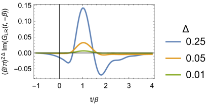
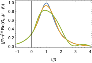
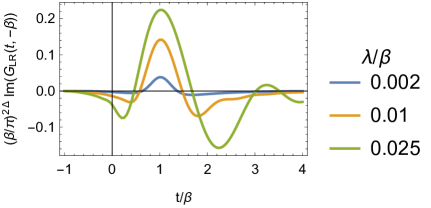
GLR(t1,t2)=(πβ)2Δi8πx𝑑usech2Δ(πu)exp(u+t+/β)2i8x,x=λβtβ,formulae-sequencesubscript𝐺𝐿𝑅subscript𝑡1subscript𝑡2superscript𝜋𝛽2Δ𝑖8𝜋𝑥superscriptsubscriptdifferential-d𝑢superscriptsech2Δ𝜋𝑢superscript𝑢subscript𝑡𝛽2𝑖8𝑥𝑥𝜆𝛽subscript𝑡𝛽\displaystyle G_{LR}(t_{1},t_{2})=\left(\frac{\pi}{\beta}\right)^{2\Delta}\sqrt{\frac{i}{8\pi x}}\int_{-\infty}^{\infty}du\operatorname{sech}^{2\Delta}\left(\pi u\right)\exp\frac{(u+t_{+}/\beta)^{2}}{i8x},\quad x=\frac{\lambda}{\beta}\frac{t_{-}}{\beta}, (3.35)

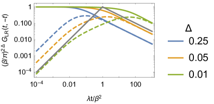
as shown in Figs. 1, 2 and 3. In Fig. 1, the peak appears near the timescale β2/λsuperscript𝛽2𝜆\beta^{2}/\lambda, which indicates the best regenesis. The correlator on the TT¯𝑇¯𝑇{T\bar{T}} deformed TFD state is

GLR(t1,t2)λ=(πβ)2Δi8πx𝑑usech2Δ(πu)exp(u+t+/β)2i8x,x=λβ(tβ+i4).formulae-sequencesubscript𝐺𝐿𝑅subscriptsubscript𝑡1subscript𝑡2𝜆superscript𝜋𝛽2Δ𝑖8𝜋𝑥superscriptsubscriptdifferential-d𝑢superscriptsech2Δ𝜋𝑢superscript𝑢subscript𝑡𝛽2𝑖8𝑥𝑥𝜆𝛽subscript𝑡𝛽𝑖4\displaystyle G_{LR}(t_{1},t_{2})_{\lambda}=\left(\frac{\pi}{\beta}\right)^{2\Delta}\sqrt{\frac{i}{8\pi x}}\int_{-\infty}^{\infty}du\operatorname{sech}^{2\Delta}\left(\pi u\right)\exp\frac{(u+t_{+}/\beta)^{2}}{i8x},\quad x=\frac{\lambda}{\beta}\left(\frac{t_{-}}{\beta}+\frac{i}{4}\right). (3.36)

The behavior is close to that in the case of the TT¯𝑇¯𝑇{T\bar{T}} quenched TFD state, except that the correlation is slightly suppressed due to the loss of entanglement.
Refer to caption
Figure 1: GLR(t,t)subscript𝐺𝐿𝑅𝑡𝑡G_{LR}(t,-t) for conformal QM, in which the real (imaginary) part is denoted as solid (dashed) line. The gray lines denote power laws t𝑡t and t1/2superscript𝑡12t^{-1/2}.
Refer to caption
Refer to caption
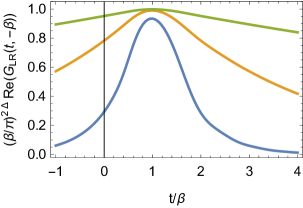
Figure 2: GLR(t,β)subscript𝐺𝐿𝑅𝑡𝛽G_{LR}(t,-\beta) for conformal QM, where λ/β=0.01𝜆𝛽0.01\lambda/\beta=0.01.
Refer to caption
Refer to caption
Figure 3: GLR(t,β)subscript𝐺𝐿𝑅𝑡𝛽G_{LR}(t,-\beta) for conformal QM, where Δ=0.25Δ0.25\Delta=0.25.

3.4.2 The SYK model

Refer to caption
Refer to caption
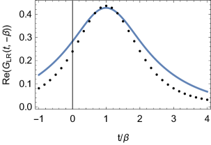
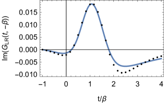
Figure 4: GLR(t,β)subscript𝐺𝐿𝑅𝑡𝛽G_{LR}(t,-\beta) for the SYK model. The dots denote the results from exact diagonalization. The curves denote the results from (3.39). The parameters are q=4,N=20,𝒥=1,β=2,λ=0.02formulae-sequence𝑞4formulae-sequence𝑁20formulae-sequence𝒥1formulae-sequence𝛽2𝜆0.02q=4,N=20,\mathcal{J}=1,\beta=2,\lambda=0.02.

We consider the SYK model as the QM system, in which the local Hamiltonian is Sachdev:2015efa ; Kitaev:2015hch ; Maldacena:2016hyu ; Kitaev:2017awl

H=iq2q!j1,,jqJj1,,jqψj1ψjq,Jj1,,jq2¯=2q1(q1)!𝒥2qNq1.formulae-sequence𝐻superscript𝑖𝑞2𝑞subscriptsubscript𝑗1subscript𝑗𝑞subscript𝐽subscript𝑗1subscript𝑗𝑞superscript𝜓subscript𝑗1superscript𝜓subscript𝑗𝑞¯superscriptsubscript𝐽subscript𝑗1subscript𝑗𝑞2superscript2𝑞1𝑞1superscript𝒥2𝑞superscript𝑁𝑞1\displaystyle H=\frac{i^{\frac{q}{2}}}{q!}\sum_{j_{1},\cdots,j_{q}}J_{j_{1},\cdots,j_{q}}\psi^{j_{1}}\cdots\psi^{j_{q}},\quad\overline{J_{j_{1},\cdots,j_{q}}^{2}}=\frac{2^{q-1}(q-1)!\mathcal{J}^{2}}{qN^{q-1}}. (3.37)

The SYK model exhibits free fermionic behavior in the UV and conformal symmetry in the infrared (IR). The two-point function interpolating between UV and IR can be solved at the large-q𝑞q limit. The Wightman function is Maldacena:2016hyu

GW(t;β)=12[(cosπv2coshπvtβ)2]1/q,πv=β𝒥cosπv2.formulae-sequencesubscript𝐺𝑊𝑡𝛽12superscriptdelimited-[]superscript𝜋𝑣2𝜋𝑣𝑡𝛽21𝑞𝜋𝑣𝛽𝒥𝜋𝑣2\displaystyle G_{W}(t;\beta)=\frac{1}{2}\left[\left(\frac{\cos\frac{\pi v}{2}}{\cosh\frac{\pi vt}{\beta}}\right)^{2}\right]^{1/q},\quad\pi v=\beta\mathcal{J}\cos\frac{\pi v}{2}. (3.38)

For the TT¯𝑇¯𝑇{T\bar{T}} quenched TFD state, the correlator at weakly coupled limit |λ|1/Eββ𝒥2/Nmuch-less-than𝜆1subscript𝐸𝛽similar-to𝛽superscript𝒥2𝑁|\lambda|\ll 1/E_{\beta}\sim\beta\mathcal{J}^{2}/N is similar to the conformal result:

GLR(t1,t2)=(πvβ𝒥)2/q12i8πx𝑑usech2/q(πvu)exp(u+t+/β)2i8x,x=λβtβ,formulae-sequencesubscript𝐺𝐿𝑅subscript𝑡1subscript𝑡2superscript𝜋𝑣𝛽𝒥2𝑞12𝑖8𝜋𝑥superscriptsubscriptdifferential-d𝑢superscriptsech2𝑞𝜋𝑣𝑢superscript𝑢subscript𝑡𝛽2𝑖8𝑥𝑥𝜆𝛽subscript𝑡𝛽\displaystyle G_{LR}(t_{1},t_{2})=\left(\frac{\pi v}{\beta\mathcal{J}}\right)^{2/q}\frac{1}{2}\sqrt{\frac{i}{8\pi x}}\int_{-\infty}^{\infty}du\operatorname{sech}^{2/q}\left(\pi vu\right)\exp\frac{(u+t_{+}/\beta)^{2}}{i8x},\quad x=\frac{\lambda}{\beta}\frac{t_{-}}{\beta}, (3.39)

which is close to the result from exact diagonalization in Fig. 4. For the TT¯𝑇¯𝑇{T\bar{T}} deformed TFD state, the correlator is

GLR(t1,t2)λ=(πvβ𝒥)2/q12i8πx𝑑usech2/q(πvu)exp(u+t+/β)2i8x,x=λβ(tβ+i4).formulae-sequencesubscript𝐺𝐿𝑅subscriptsubscript𝑡1subscript𝑡2𝜆superscript𝜋𝑣𝛽𝒥2𝑞12𝑖8𝜋𝑥superscriptsubscriptdifferential-d𝑢superscriptsech2𝑞𝜋𝑣𝑢superscript𝑢subscript𝑡𝛽2𝑖8𝑥𝑥𝜆𝛽subscript𝑡𝛽𝑖4\displaystyle G_{LR}(t_{1},t_{2})_{\lambda}=\left(\frac{\pi v}{\beta\mathcal{J}}\right)^{2/q}\frac{1}{2}\sqrt{\frac{i}{8\pi x}}\int_{-\infty}^{\infty}du\operatorname{sech}^{2/q}\left(\pi vu\right)\exp\frac{(u+t_{+}/\beta)^{2}}{i8x},\quad x=\frac{\lambda}{\beta}\left(\frac{t_{-}}{\beta}+\frac{i}{4}\right). (3.40)

3.4.3 The system satisfying the ETH

We can apply the above formula to the system satisfying the ETH. Consider the Hermitian operator O𝑂O which satisfies Feingold:1986fu ; Deutsch:1991qsm ; Srednicki:1994cqt ; Srednicki:1995qcs

Oab1DF(E+,E)Rab,ab,formulae-sequencesubscript𝑂𝑎𝑏1𝐷𝐹subscript𝐸subscript𝐸subscript𝑅𝑎𝑏𝑎𝑏\displaystyle O_{ab}\approx\frac{1}{\sqrt{D}}F(E_{+},E_{-})R_{ab},\quad a\neq b, (3.41)
Rab=0,RabRcd=δacδbd,E±=Ea±Eb,formulae-sequencedelimited-⟨⟩subscript𝑅𝑎𝑏0formulae-sequencedelimited-⟨⟩subscript𝑅𝑎𝑏superscriptsubscript𝑅𝑐𝑑subscript𝛿𝑎𝑐subscript𝛿𝑏𝑑subscript𝐸plus-or-minusplus-or-minussubscript𝐸𝑎subscript𝐸𝑏\displaystyle\left\langle R_{ab}\right\rangle=0,\quad\left\langle R_{ab}R_{cd}^{*}\right\rangle=\delta_{ac}\delta_{bd},\quad E_{\pm}=E_{a}\pm E_{b}, (3.42)

where Rabsubscript𝑅𝑎𝑏R_{ab} is a random matrix. We further assume that the operator O𝑂O has bandwidth ΓΓ\Gamma:

F(E+,E)A(E+/2)e|E|/Γ.similar-to𝐹subscript𝐸subscript𝐸𝐴subscript𝐸2superscript𝑒subscript𝐸Γ\displaystyle F(E_{+},E_{-})\sim A(E_{+}/2)e^{-|E_{-}|/\Gamma}. (3.43)

The off-diagonal part of the correlator of the operator on the TT¯𝑇¯𝑇{T\bar{T}} quenched TFD state is

Ψ|OL(t1)OR(t2)|ΨaOaa2exp{βEa}quantum-operator-productΨsubscript𝑂𝐿subscript𝑡1subscript𝑂𝑅subscript𝑡2Ψsubscript𝑎superscriptsubscript𝑂𝑎𝑎2𝛽subscript𝐸𝑎\displaystyle\left\langle\Psi\right|O_{L}(t_{1})O_{R}(t_{2})\left|\Psi\right\rangle-\sum_{a}O_{aa}^{2}\exp\left\{-\beta E_{a}\right\} (3.44)
=\displaystyle= 1DabRabRbaA(E+2)2exp{β2E++2iλtE2+it+(1+4λE+)E2Γ|E|}1𝐷subscript𝑎𝑏delimited-⟨⟩subscript𝑅𝑎𝑏subscript𝑅𝑏𝑎𝐴superscriptsubscript𝐸22𝛽2subscript𝐸2𝑖𝜆subscript𝑡superscriptsubscript𝐸2𝑖subscript𝑡14𝜆subscript𝐸subscript𝐸2Γsubscript𝐸\displaystyle\frac{1}{D}\sum_{a\neq b}\left\langle R_{ab}R_{ba}\right\rangle A\left(\frac{E_{+}}{2}\right)^{2}\exp\left\{-\frac{\beta}{2}E_{+}+2i\lambda t_{-}E_{-}^{2}+it_{+}(1+4\lambda E_{+})E_{-}-\frac{2}{\Gamma}|E_{-}|\right\} (3.45)
\displaystyle\approx 1DabA(E+2)2exp{β2E++2iλtE2+it+E2Γ|E|}1𝐷subscript𝑎𝑏𝐴superscriptsubscript𝐸22𝛽2subscript𝐸2𝑖𝜆subscript𝑡superscriptsubscript𝐸2𝑖subscript𝑡subscript𝐸2Γsubscript𝐸\displaystyle\frac{1}{D}\sum_{a\neq b}A\left(\frac{E_{+}}{2}\right)^{2}\exp\left\{-\frac{\beta}{2}E_{+}+2i\lambda t_{-}E_{-}^{2}+it_{+}E_{-}-\frac{2}{\Gamma}|E_{-}|\right\} (3.46)

based on the weakly coupled limit |λ|1/Eβmuch-less-than𝜆1subscript𝐸𝛽|\lambda|\ll 1/E_{\beta}. For large D𝐷D, the energy band Λ=EmaxEminΛsubscript𝐸subscript𝐸\Lambda=E_{\max}-E_{\min} is much larger than the bandwidth ΓΓ\Gamma. So we can calculate the integral in the approximation of flat spectrum difference as

abD20Λ𝑑Ea𝑑Ebρ(Ea)ρ(Eb)D202Λ𝑑E+ρ(E+/2)+𝑑E.subscript𝑎𝑏superscript𝐷2superscriptsubscript0Λdifferential-dsubscript𝐸𝑎differential-dsubscript𝐸𝑏𝜌subscript𝐸𝑎𝜌subscript𝐸𝑏superscript𝐷2superscriptsubscript02Λdifferential-dsubscript𝐸𝜌subscript𝐸2superscriptsubscriptdifferential-dsubscript𝐸\displaystyle\sum_{a\neq b}\approx D^{2}\int_{0}^{\Lambda}dE_{a}dE_{b}\,\rho(E_{a})\rho(E_{b})\approx D^{2}\int_{0}^{2\Lambda}dE_{+}\,\rho(E_{+}/2)\int_{-\infty}^{+\infty}dE_{-}. (3.47)

Then, the off-diagonal part is simplified as

D02Λ𝑑E+A(E+2)2ρ(E+2)exp{β2E+}+𝑑Eexp{2iλtE2+it+E2Γ|E|}𝐷superscriptsubscript02Λdifferential-dsubscript𝐸𝐴superscriptsubscript𝐸22𝜌subscript𝐸2𝛽2subscript𝐸superscriptsubscriptdifferential-dsubscript𝐸2𝑖𝜆subscript𝑡superscriptsubscript𝐸2𝑖subscript𝑡subscript𝐸2Γsubscript𝐸\displaystyle D\int_{0}^{2\Lambda}dE_{+}\,A\left(\frac{E_{+}}{2}\right)^{2}\rho\left(\frac{E_{+}}{2}\right)\exp\left\{-\frac{\beta}{2}E_{+}\right\}\int_{-\infty}^{+\infty}dE_{-}\exp\left\{2i\lambda t_{-}E_{-}^{2}+it_{+}E_{-}-\frac{2}{\Gamma}|E_{-}|\right\}
=\displaystyle= 2[D0Λ𝑑EA(E)2ρ(E)eβE]π8iλt[g(2/Γit+8iλt)+g(2/Γ+it+8iλt)],2delimited-[]𝐷superscriptsubscript0Λdifferential-d𝐸𝐴superscript𝐸2𝜌𝐸superscript𝑒𝛽𝐸𝜋8𝑖𝜆subscript𝑡delimited-[]𝑔2Γ𝑖subscript𝑡8𝑖𝜆subscript𝑡𝑔2Γ𝑖subscript𝑡8𝑖𝜆subscript𝑡\displaystyle 2\left[D\int_{0}^{\Lambda}dE\,A(E)^{2}\rho(E)e^{-\beta E}\right]\sqrt{\frac{\pi}{-8i\lambda t_{-}}}\left[g\left(\frac{2/\Gamma-it_{+}}{\sqrt{-8i\lambda t_{-}}}\right)+g\left(\frac{2/\Gamma+it_{+}}{\sqrt{-8i\lambda t_{-}}}\right)\right], (3.48)

where

g(z)=ez2erfc(z)=ez2(12π0z𝑑xex2).𝑔𝑧superscript𝑒superscript𝑧2erfc𝑧superscript𝑒superscript𝑧212𝜋superscriptsubscript0𝑧differential-d𝑥superscript𝑒superscript𝑥2\displaystyle g(z)=e^{z^{2}}\text{erfc}(z)=e^{z^{2}}\left(1-\frac{2}{\sqrt{\pi}}\int_{0}^{z}dxe^{-x^{2}}\right). (3.49)

Let A2=Z[β]1D0Λ𝑑EA(E)2ρ(E)eβEsuperscript𝐴2𝑍superscriptdelimited-[]𝛽1𝐷superscriptsubscript0Λdifferential-d𝐸𝐴superscript𝐸2𝜌𝐸superscript𝑒𝛽𝐸A^{2}=Z[\beta]^{-1}D\int_{0}^{\Lambda}dE\,A(E)^{2}\rho(E)e^{-\beta E}. The retarded correlator is

GLRR(t1,t2)4A2Im{πi8λt[g(2/Γit+8iλt)+g(2/Γ+it+8iλt)]}.superscriptsubscript𝐺𝐿𝑅𝑅subscript𝑡1subscript𝑡24superscript𝐴2Im𝜋𝑖8𝜆subscript𝑡delimited-[]𝑔2Γ𝑖subscript𝑡8𝑖𝜆subscript𝑡𝑔2Γ𝑖subscript𝑡8𝑖𝜆subscript𝑡\displaystyle G_{LR}^{R}(t_{1},t_{2})\approx 4A^{2}{\rm Im}\left\{\sqrt{\frac{\pi}{-i8\lambda t_{-}}}\left[g\left(\frac{2/\Gamma-it_{+}}{\sqrt{-8i\lambda t_{-}}}\right)+g\left(\frac{2/\Gamma+it_{+}}{\sqrt{-8i\lambda t_{-}}}\right)\right]\right\}. (3.50)

Asymptotically,

GLRR(t,t)2A2{32Γ3λt43Γ2t+2(4+Γ2t+2)3,t0πλt,t.\displaystyle G_{LR}^{R}(t,-t)\to 2A^{2}\begin{cases}32\Gamma^{3}\lambda t_{-}\frac{4-3\Gamma^{2}t_{+}^{2}}{(4+\Gamma^{2}t_{+}^{2}){}^{3}},&t_{-}\to 0\\ \sqrt{\frac{\pi}{\lambda t_{-}}},&t_{-}\to\infty\end{cases}. (3.51)

whose exponents are the same as the conformal result in Fig. 1.

By replacing ititβ4𝑖subscript𝑡𝑖subscript𝑡𝛽4it_{-}\to it_{-}-\frac{\beta}{4}, we obtain the retarded correlator of the TT¯𝑇¯𝑇{T\bar{T}} deformed TFD state as

GLRR(t1,t2)λ4A2Im{π2λ(β4it)[g(2/Γit+2λ(β4it))+g(2/Γ+it+2λ(β4it))]}.superscriptsubscript𝐺𝐿𝑅𝑅subscriptsubscript𝑡1subscript𝑡2𝜆4superscript𝐴2Im𝜋2𝜆𝛽4𝑖subscript𝑡delimited-[]𝑔2Γ𝑖subscript𝑡2𝜆𝛽4𝑖subscript𝑡𝑔2Γ𝑖subscript𝑡2𝜆𝛽4𝑖subscript𝑡\displaystyle G_{LR}^{R}(t_{1},t_{2})_{\lambda}\approx 4A^{2}{\rm Im}\left\{\sqrt{\frac{\pi}{2\lambda(\beta-4it_{-})}}\left[g\left(\frac{2/\Gamma-it_{+}}{\sqrt{2\lambda(\beta-4it_{-})}}\right)+g\left(\frac{2/\Gamma+it_{+}}{\sqrt{2\lambda(\beta-4it_{-})}}\right)\right]\right\}. (3.52)

4 TT¯𝑇¯𝑇{T\bar{T}} deformation on Schwarzian theory

In this section, we consider the TT¯𝑇¯𝑇{T\bar{T}} deformation on an eternal black hole in Jackiw-Teitelboim (JT) gravity as Maldacena:2016upp ; Engelsoy:2016xyb

I=116πG[d2xgΦ(R+2)+2b𝑑xhΦb(K1)]𝐼116𝜋𝐺delimited-[]superscript𝑑2𝑥𝑔Φ𝑅22subscript𝑏differential-d𝑥subscriptΦ𝑏𝐾1\displaystyle I=\frac{1}{16\pi G}\left[\int d^{2}x\sqrt{-g}\Phi(R+2)+2\int_{b}dx\sqrt{-h}\Phi_{b}(K-1)\right] (4.1)

with the boundary condition

dsh2=dt2/ϵ2,Φb=Φr/ϵ,formulae-sequence𝑑subscriptsuperscript𝑠2𝑑superscript𝑡2superscriptitalic-ϵ2subscriptΦ𝑏subscriptΦ𝑟italic-ϵ\displaystyle ds^{2}_{h}=-dt^{2}/\epsilon^{2},\quad\Phi_{b}=\Phi_{r}/\epsilon, (4.2)

where b𝑏b denotes the boundary, hh is the induced metric on the boundary, ΦbsubscriptΦ𝑏\Phi_{b} is the value of the dilaton ΦΦ\Phi on the boundary, and ϵitalic-ϵ\epsilon is the UV cutoff. We have introduced a counterterm to cancel the divergence in the exterior curvature K𝐾K. By integrating out the dilaton ΦΦ\Phi, we have R+2=0𝑅20R+2=0. The solution is an AdS2 space. In the global coordinate and the Rindler coordinate, the metric reads

ds2=dν2+dσ2sin2σ=sinh2ρdφ2+dρ2.𝑑superscript𝑠2𝑑superscript𝜈2𝑑superscript𝜎2superscript2𝜎superscript2𝜌𝑑superscript𝜑2𝑑superscript𝜌2\displaystyle ds^{2}=\frac{-d\nu^{2}+d\sigma^{2}}{\sin^{2}\sigma}=-\sinh^{2}\rho d\varphi^{2}+d\rho^{2}. (4.3)

We consider two boundaries L𝐿L and R𝑅R with reparametrization (φL(t),ρL(t))subscript𝜑𝐿𝑡subscript𝜌𝐿𝑡\left(\varphi_{L}(t),\rho_{L}(t)\right) and (φR(t),ρR(t))subscript𝜑𝑅𝑡subscript𝜌𝑅𝑡\left(\varphi_{R}(t),\rho_{R}(t)\right) respectively. To satisfy the boundary condition, the reparametrizations are expanded as

sinhρL(t)=subscript𝜌𝐿𝑡absent\displaystyle\sinh\rho_{L}(t)= 1ϵφL(t)ϵφL′′(t)22φL(t)3+𝒪(ϵ2),1italic-ϵsuperscriptsubscript𝜑𝐿𝑡italic-ϵsuperscriptsubscript𝜑𝐿′′superscript𝑡22superscriptsubscript𝜑𝐿superscript𝑡3𝒪superscriptitalic-ϵ2\displaystyle-\frac{1}{\epsilon\varphi_{L}^{\prime}(t)}-\frac{\epsilon\varphi_{L}^{\prime\prime}(t)^{2}}{2\varphi_{L}^{\prime}(t)^{3}}+\mathcal{O}(\epsilon^{2}), (4.4)
sinhρR(t)=subscript𝜌𝑅𝑡absent\displaystyle\sinh\rho_{R}(t)= 1ϵφR(t)+ϵφR′′(t)22φR(t)3+𝒪(ϵ2).1italic-ϵsuperscriptsubscript𝜑𝑅𝑡italic-ϵsuperscriptsubscript𝜑𝑅′′superscript𝑡22superscriptsubscript𝜑𝑅superscript𝑡3𝒪superscriptitalic-ϵ2\displaystyle\frac{1}{\epsilon\varphi_{R}^{\prime}(t)}+\frac{\epsilon\varphi_{R}^{\prime\prime}(t)^{2}}{2\varphi_{R}^{\prime}(t)^{3}}+\mathcal{O}(\epsilon^{2}). (4.5)

The action is then reduced to the two-sited Schwarzian theory:

I=𝐼absent\displaystyle I= 18πGL,R𝑑xhΦb(K1)18𝜋𝐺subscript𝐿𝑅differential-d𝑥subscriptΦ𝑏𝐾1\displaystyle\frac{1}{8\pi G}\int_{L,R}dx\sqrt{-h}\Phi_{b}(K-1) (4.6)
=\displaystyle= C𝑑t[Sch(cothφL2,u)+Sch(tanhφR2,u)]+𝒪[ϵ2]𝐶differential-d𝑡delimited-[]Schhyperbolic-cotangentsubscript𝜑𝐿2𝑢Schsubscript𝜑𝑅2𝑢𝒪delimited-[]superscriptitalic-ϵ2\displaystyle-C\int dt\left[{\text{Sch}}\left(-\coth\frac{\varphi_{L}}{2},u\right)+{\text{Sch}}\left(\tanh\frac{\varphi_{R}}{2},u\right)\right]+\mathcal{O}[\epsilon^{2}] (4.7)
=\displaystyle= C2dt[φL′′(t)2φL(t)2+φL(t)+2φR′′(t)2φR(t)2+φR(t)]2+surface term,C=Φr8πG.\displaystyle\frac{C}{2}\int dt\left[\frac{\varphi_{L}^{\prime\prime}(t){}^{2}}{\varphi_{L}^{\prime}(t){}^{2}}+\varphi_{L}^{\prime}(t){}^{2}+\frac{\varphi_{R}^{\prime\prime}(t){}^{2}}{\varphi_{R}^{\prime}(t){}^{2}}+\varphi_{R}^{\prime}(t){}^{2}\right]+\text{surface term},\quad C=\frac{\Phi_{r}}{8\pi G}. (4.8)

Similar to the argument presented in Maldacena:2018lmt , the action has SL(2) gauge symmetry, and the gauge charges vanish. Therefore, the solution can be transformed into the LR𝐿𝑅LR-symmetric form φL(u)=φR(t)=φ(t)subscript𝜑𝐿𝑢subscript𝜑𝑅𝑡𝜑𝑡\varphi_{L}(u)=\varphi_{R}(t)=\varphi(t). Following Gross:2019ach , we will consider the TT¯𝑇¯𝑇{T\bar{T}} deformation and use Ostrogradsky formalism to write down the canonical variables Woodard:2015zca

q1=φ,q1=φ,p1=LφtLφ′′=C[φ′′2φ3+φφ(3)φ2],p2=Lφ′′=Cφ′′φ2.\begin{split}&q_{1}=\varphi,\quad q_{1}=\varphi^{\prime},\\ &p_{1}=\frac{\partial L}{\partial\varphi^{\prime}}-\partial_{t}\frac{\partial L}{\partial\varphi^{\prime\prime}}=C\left[\frac{\varphi^{\prime\prime 2}}{\varphi^{\prime 3}}+\varphi^{\prime}-\frac{\varphi^{(3)}}{\varphi^{\prime 2}}\right],\quad p_{2}=\frac{\partial L}{\partial\varphi^{\prime\prime}}=C\frac{\varphi^{\prime\prime}}{\varphi^{\prime 2}}.\end{split} (4.9)

The Hamiltonian in Ostrogradsky formalism is

H0=HL+HR=p1q2+14Cp22q22Cq22.subscript𝐻0subscript𝐻𝐿subscript𝐻𝑅subscript𝑝1subscript𝑞214𝐶superscriptsubscript𝑝22superscriptsubscript𝑞22𝐶superscriptsubscript𝑞22\displaystyle H_{0}=H_{L}+H_{R}=p_{1}q_{2}+\frac{1}{4C}p_{2}^{2}q_{2}^{2}-Cq_{2}^{2}. (4.10)

The solution of the TFD state at inverse temperature β𝛽\beta is

φ(t)=φβ(t)=2πtβ,𝜑𝑡subscript𝜑𝛽𝑡2𝜋𝑡𝛽\displaystyle\varphi(t)=\varphi_{\beta}(t)=\frac{2\pi t}{\beta}, (4.11)

and all the canonical variables are determined by (4.9). With (4.4) and (4.5), the solution of the reparametrization describes two boundary trajectories on the constant radius in the Rindler patch of AdS2 space, which corresponds to a wormhole connecting the two boundaries from a higher-dimensional perspective.

We first consider a general deformation:

Hλ=f(H0).subscript𝐻𝜆𝑓subscript𝐻0\displaystyle H_{\lambda}=f(H_{0}). (4.12)

Under the deformation, the canonical relations are determined by the deformed Hamiltonian equation as

qi=Hλpi,pi=Hλqi.formulae-sequencesubscriptsuperscript𝑞𝑖subscript𝐻𝜆subscriptsuperscript𝑝𝑖subscriptsuperscript𝑝𝑖subscript𝐻𝜆subscriptsuperscript𝑞𝑖\displaystyle q^{\prime}_{i}=\frac{\partial H_{\lambda}}{\partial p^{\prime}_{i}},\quad p^{\prime}_{i}=-\frac{\partial H_{\lambda}}{\partial q^{\prime}_{i}}. (4.13)

Given a solution of the Hamiltonian equation of H0subscript𝐻0H_{0}, such as the φβ(t)subscript𝜑𝛽𝑡\varphi_{\beta}(t) in (4.11), we can find a solution of Hλsubscript𝐻𝜆H_{\lambda} from (2.5). We introduce the dynamical time as

T=kt,k=f(H0[φβ(t)]),formulae-sequence𝑇𝑘𝑡𝑘superscript𝑓subscript𝐻0delimited-[]subscript𝜑𝛽𝑡\displaystyle T=kt,\quad k=f^{\prime}(H_{0}[\varphi_{\beta}(t)]), (4.14)

where H0[φβ(t)]=4π2C/β2subscript𝐻0delimited-[]subscript𝜑𝛽𝑡4superscript𝜋2𝐶superscript𝛽2H_{0}[\varphi_{\beta}(t)]=4\pi^{2}C/\beta^{2} refers to the value of H0subscript𝐻0H_{0} on the canonical variables determined by the solution in (4.11) with the canonical relation in (4.9). A solution of the Hamiltonian equation of Hλsubscript𝐻𝜆H_{\lambda} is

φ(t)=φβ(kt)=φβ/k(t)=2πkt/β,𝜑𝑡subscript𝜑𝛽𝑘𝑡subscript𝜑𝛽𝑘𝑡2𝜋𝑘𝑡𝛽\displaystyle\varphi(t)=\varphi_{\beta}(kt)=\varphi_{\beta/k}(t)=2\pi kt/\beta, (4.15)
q1=2πkt/β,q2=2π/β,p1=2πC/β,p2=0,formulae-sequencesubscript𝑞12𝜋𝑘𝑡𝛽formulae-sequencesubscript𝑞22𝜋𝛽formulae-sequencesubscript𝑝12𝜋𝐶𝛽subscript𝑝20\displaystyle q_{1}=2\pi kt/\beta,\quad q_{2}=2\pi/\beta,\quad p_{1}=2\pi C/\beta,\quad p_{2}=0, (4.16)

and the energy is Hλ[φβ(kt)]=f(4π2C/β2)subscript𝐻𝜆delimited-[]subscript𝜑𝛽𝑘𝑡𝑓4superscript𝜋2𝐶superscript𝛽2H_{\lambda}[\varphi_{\beta}(kt)]=f(4\pi^{2}C/\beta^{2}).

We select the TT¯𝑇¯𝑇{T\bar{T}} deformation as

Hλ=f(H0)=118H0λ4λ.subscript𝐻𝜆𝑓subscript𝐻0118subscript𝐻0𝜆4𝜆\displaystyle H_{\lambda}=f(H_{0})=\frac{1-\sqrt{1-8H_{0}\lambda}}{4\lambda}. (4.17)

Then, k=1/132π2λC/β2𝑘1132superscript𝜋2𝜆𝐶superscript𝛽2k=1/\sqrt{1-32\pi^{2}\lambda C/\beta^{2}} and Hλ[φβ(kt)]=(1132π2λC/β2)/4λsubscript𝐻𝜆delimited-[]subscript𝜑𝛽𝑘𝑡1132superscript𝜋2𝜆𝐶superscript𝛽24𝜆H_{\lambda}[\varphi_{\beta}(kt)]=\left(1-\sqrt{1-32\pi^{2}\lambda C/\beta^{2}}\right)/4\lambda. So, the weakly coupled limit in Sec. 3 means |λ|β2/Cmuch-less-than𝜆superscript𝛽2𝐶|\lambda|\ll\beta^{2}/C and k1𝑘1k\approx 1 here.

The solution (4.15) has two interpretations that correspond to the two strategies separately in Sec. 3. First, recall that the local state ρ(t)𝜌𝑡\rho(t) in (3.7) is a thermal state of the undeformed Hamiltonian H0subscript𝐻0H_{0}. Thus, the solution φ(t)=φβ/k(t)𝜑𝑡subscript𝜑𝛽𝑘𝑡\varphi(t)=\varphi_{\beta/k}(t) is interpreted as the TT¯𝑇¯𝑇{T\bar{T}} quenched TFD state |Ψ(t)ketΨ𝑡\left|\Psi(t)\right\rangle at the inverse temperature β/k𝛽𝑘\beta/k in (3.6). Second, recall that the local state ρλ(t)subscript𝜌𝜆𝑡\rho_{\lambda}(t) in (3.28) is a thermal state of the deformed Hamiltonian f(H0)𝑓subscript𝐻0f(H_{0}), in which the dynamical time is kt𝑘𝑡kt as well. Thus, the solution φ(t)=φβ(kt)𝜑𝑡subscript𝜑𝛽𝑘𝑡\varphi(t)=\varphi_{\beta}(kt) is interpreted as the TT¯𝑇¯𝑇{T\bar{T}} deformed TFD state |Ψλ(t)ketsubscriptΨ𝜆𝑡\left|\Psi_{\lambda}(t)\right\rangle at the inverse temperature β𝛽\beta in (3.27).

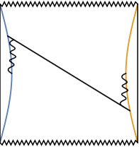
The deformed solution (4.15) is related to the undeformed solution (4.11) by rescaling the time. By plugging (4.15) into (4.4) and (4.5) respectively, we know that the TT¯𝑇¯𝑇{T\bar{T}} deformation moves the two boundaries into the bulk but keeps them spacelike separated, which agrees with the fact that the deformation is irrelevant. Thus, the causal correlation found in Sec. 3 is not associated with the causal structure of a semiclassical wormhole and is instead similar to the “quantum traversable wormhole” 111Notice that the traversability of the semiclassical traversable wormholes in Ref. Gao:2016bin is different from the traversability of the “quantum traversable wormhole” in Ref. Gao:2018yzk . The former happens after the scrambling time and is related to the spacetime structure of the bulk. The latter occurs in the interference regime much later than the scrambling time. It is generated by the superposition of the bulk states and is not related to the spacetime structure. in Ref. Gao:2018yzk . Without the TT¯𝑇¯𝑇{T\bar{T}} deformation, the vanishing of the retarded correlator is originated from the perfect cancellation between the two propagators OL(0)OR(0)delimited-⟨⟩superscriptsubscript𝑂𝐿0superscriptsubscript𝑂𝑅0\left\langle O_{L}^{(0)}O_{R}^{(0)}\right\rangle and OR(0)OL(0)delimited-⟨⟩superscriptsubscript𝑂𝑅0superscriptsubscript𝑂𝐿0\left\langle O_{R}^{(0)}O_{L}^{(0)}\right\rangle, which are dual to the process of a virtual particle traveling from R𝑅R to L𝐿L and from L𝐿L to R𝑅R in bulk respectively. With the TT¯𝑇¯𝑇{T\bar{T}} deformation, the virtual particle can release two gravitons that annihilate on the boundaries via the HLHRsubscript𝐻𝐿subscript𝐻𝑅H_{L}H_{R} term in the TT¯𝑇¯𝑇{T\bar{T}} deformation, as shown in Fig. 5. The propagators acquire different factors, resulting in the propagation of real particles.

More precisely, we can directly calculate retarded correlator GLRR(t1,t2)subscriptsuperscript𝐺𝑅𝐿𝑅subscript𝑡1subscript𝑡2G^{R}_{LR}(t_{1},t_{2}) at the first order of λ𝜆\lambda by using the Schwarzian action. Taking the GLRR(t1,t2)subscriptsuperscript𝐺𝑅𝐿𝑅subscript𝑡1subscript𝑡2G^{R}_{LR}(t_{1},t_{2}) in (3.23) as an example, where the TT¯𝑇¯𝑇{T\bar{T}} quench is applied instantaneously, we consider the reparametrization mode φ(t)=t+ε(t)𝜑𝑡𝑡𝜀𝑡\varphi(t)=t+\varepsilon(t) and expand the dynamical part of the Euclidean Schwarzian action, the correlator, and the nonlocal TT¯𝑇¯𝑇{T\bar{T}} term with respect to ε(t)𝜀𝑡\varepsilon(t) as

Iε=subscript𝐼𝜀absent\displaystyle I_{\varepsilon}= C2𝑑τ(ε′′(τ)2ε(τ)2+𝒪[ε3]),𝐶2differential-d𝜏superscript𝜀′′superscript𝜏2superscript𝜀superscript𝜏2𝒪delimited-[]superscript𝜀3\displaystyle\frac{C}{2}\int d\tau\left(\varepsilon^{\prime\prime}(\tau)^{2}-\varepsilon^{\prime}(\tau)^{2}+\mathcal{O}[\varepsilon^{3}]\right), (4.18)
O(τ1)O(τ2)=delimited-⟨⟩𝑂subscript𝜏1𝑂subscript𝜏2absent\displaystyle\left\langle O(\tau_{1})O(\tau_{2})\right\rangle= [(1+ε(τ1))(1+ε(τ2))4csc2τ1τ2+ε(τ1)ε(τ2)2]Δ,superscriptdelimited-[]1superscript𝜀subscript𝜏11superscript𝜀subscript𝜏24superscript2subscript𝜏1subscript𝜏2𝜀subscript𝜏1𝜀subscript𝜏22Δ\displaystyle\left[\frac{\left(1+\varepsilon^{\prime}(\tau_{1})\right)\left(1+\varepsilon^{\prime}(\tau_{2})\right)}{4}\csc^{2}\frac{\tau_{1}-\tau_{2}+\varepsilon(\tau_{1})-\varepsilon(\tau_{2})}{2}\right]^{\Delta}, (4.19)
4λHLHR=4𝜆subscript𝐻𝐿subscript𝐻𝑅absent\displaystyle-4\lambda H_{L}H_{R}= 𝒪[ε]4λC2(ε(3)(0)+ε(0))(ε(3)(π)+ε(π))+𝒪[ε3],β=2π.𝒪delimited-[]𝜀4𝜆superscript𝐶2superscript𝜀30superscript𝜀0superscript𝜀3𝜋superscript𝜀𝜋𝒪delimited-[]superscript𝜀3𝛽2𝜋\displaystyle\mathcal{O}[\varepsilon]-4\lambda C^{2}\left(\varepsilon^{(3)}(0)+\varepsilon^{\prime}(0)\right)\left(\varepsilon^{(3)}(\pi)+\varepsilon^{\prime}(\pi)\right)+\mathcal{O}[\varepsilon^{3}],\quad\beta=2\pi. (4.20)

The quadratic term in Iεsubscript𝐼𝜀I_{\varepsilon} gives the propagator of reparametrization model ε(τ)ε=(π|τ|)(π|τ|+2sin|τ|)/(4πC)delimited-⟨⟩𝜀𝜏𝜀𝜋𝜏𝜋𝜏2𝜏4𝜋𝐶\left\langle\varepsilon(\tau)\varepsilon\right\rangle=-(\pi-|\tau|)(\pi-|\tau|+2\sin|\tau|)/(4\pi C) Maldacena:2016upp . The brackets εεεεdelimited-⟨⟩𝜀𝜀𝜀𝜀\left\langle\varepsilon\varepsilon\varepsilon\varepsilon\right\rangle in the commutator 4λ[[HLHR,OL(t1)],O(t2)]4𝜆delimited-⟨⟩subscript𝐻𝐿subscript𝐻𝑅subscript𝑂𝐿subscript𝑡1𝑂subscript𝑡2-4\lambda\langle[[H_{L}H_{R},O_{L}(t_{1})],O(t_{2})]\rangle are factorized into εεεε,delimited-⟨⟩𝜀𝜀delimited-⟨⟩𝜀𝜀\left\langle\varepsilon\varepsilon\right\rangle\left\langle\varepsilon\varepsilon\right\rangle, as shown in Fig. 5. The 𝒪[ε3]𝒪delimited-[]superscript𝜀3\mathcal{O}[\varepsilon^{3}] term in Iεsubscript𝐼𝜀I_{\varepsilon} and the 𝒪[ε]𝒪delimited-[]𝜀\mathcal{O}[\varepsilon] term in 4λHLHR4𝜆subscript𝐻𝐿subscript𝐻𝑅-4\lambda H_{L}H_{R} do not contribute to the commutator. The final result is (3.24) at the tree level.

By Legendre transforming the deformed Hamiltonian and letting q1=φ,q2=eϕformulae-sequencesubscript𝑞1𝜑subscript𝑞2superscript𝑒italic-ϕq_{1}=\varphi,\ q_{2}=e^{\phi}, we obtain the deformed Lagrangian as

λ=Ceϕ(φ2+ϕ2)φ+(eϕφ)28λφeϕ.subscript𝜆𝐶superscript𝑒italic-ϕsuperscript𝜑2superscriptitalic-ϕ2superscript𝜑superscriptsuperscript𝑒italic-ϕsuperscript𝜑28𝜆superscript𝜑superscript𝑒italic-ϕ\displaystyle\mathcal{L}_{\lambda}=\frac{Ce^{\phi}\left(\varphi^{\prime 2}+\phi^{\prime 2}\right)}{\varphi^{\prime}}+\frac{\left(e^{\phi}-\varphi^{\prime}\right)^{2}}{8\lambda\varphi^{\prime}e^{\phi}}. (4.21)

Solving φ𝜑\varphi and substituting it in the Lagrangian, we have

λ=(1+8Cλϕ2)(1+8Cλe2ϕ)14λ,subscript𝜆18𝐶𝜆superscriptitalic-ϕ218𝐶𝜆superscript𝑒2italic-ϕ14𝜆\displaystyle\mathcal{L}_{\lambda}=\frac{\sqrt{\left(1+8C\lambda\phi^{\prime 2}\right)\left(1+8C\lambda e^{2\phi}\right)}-1}{4\lambda}, (4.22)

which agrees with the TT¯𝑇¯𝑇{T\bar{T}} deformation of the Liouville QM =C2(ϕL2+ϕL2+e2ϕL+e2ϕR)𝐶2superscriptsubscriptitalic-ϕ𝐿2superscriptsubscriptitalic-ϕ𝐿2superscript𝑒2subscriptitalic-ϕ𝐿superscript𝑒2subscriptitalic-ϕ𝑅\mathcal{L}=\frac{C}{2}(\phi_{L}^{\prime 2}+\phi_{L}^{\prime 2}+e^{2\phi_{L}}+e^{2\phi_{R}}) when ϕL=ϕR=ϕsubscriptitalic-ϕ𝐿subscriptitalic-ϕ𝑅italic-ϕ\phi_{L}=\phi_{R}=\phi, as given in (2.22).

To keep the correction of finite cutoff ϵitalic-ϵ\epsilon, we substitute (4.4) and (4.5) into the action (4.6) and obtain the Lagrangian as

ϵ=Cs=L,R12(φs+2φs′′22φs2)+ϵ28(57φs′′4φs4φs+48φs′′′2φs26φs′′)2+𝒪[ϵ3].\displaystyle\mathcal{L}_{\epsilon}=C\sum_{s=L,R}\frac{1}{2}\left(\varphi_{s}^{\prime}{}^{2}+\frac{\varphi_{s}^{\prime\prime}{}^{2}}{2\varphi_{s}^{\prime}{}^{2}}\right)+\frac{\epsilon^{2}}{8}\left(-\frac{57\varphi_{s}^{\prime\prime}{}^{4}}{\varphi_{s}^{\prime}{}^{4}}-\varphi_{s}^{\prime}{}^{4}+\frac{8\varphi_{s}^{\prime\prime\prime}{}^{2}}{\varphi_{s}^{\prime}{}^{2}}-6\varphi_{s}^{\prime\prime}{}^{2}\right)+\mathcal{O}\left[\epsilon^{3}\right]. (4.23)

Substituting the solution (4.11) in the above Lagrangian, we get ϵ=4π2Cβ216π4C2λ/β4subscriptitalic-ϵ4superscript𝜋2𝐶superscript𝛽216superscript𝜋4superscript𝐶2𝜆superscript𝛽4\mathcal{L}_{\epsilon}=4\pi^{2}C\beta^{-2}-16\pi^{4}C^{2}\lambda/\beta^{-4}, where we use λ=2πϵ2G/ΦR𝜆2𝜋superscriptitalic-ϵ2𝐺subscriptΦ𝑅\lambda=2\pi\epsilon^{2}G/\Phi_{R}, based on Hartman:2018tkw ; Gross:2019uxi . However, if we substitute the deformed solution (4.15) into (4.22), we get λ=4π2Cβ232π4C2λ/β4subscript𝜆4superscript𝜋2𝐶superscript𝛽232superscript𝜋4superscript𝐶2𝜆superscript𝛽4\mathcal{L}_{\lambda}=4\pi^{2}C\beta^{-2}-32\pi^{4}C^{2}\lambda/\beta^{-4}, which is different form ϵsubscriptitalic-ϵ\mathcal{L}_{\epsilon}. Therefore, the effect of the nonlocal TT¯𝑇¯𝑇{T\bar{T}} deformation considered in this study is not simply equivalent to moving the boundaries into the bulk McGough:2016lol . Rather, it couples the two boundaries and leads to nonlocal dynamics.
Refer to caption
Figure 5: Witten diagram in retarded correlator GLRRsubscriptsuperscript𝐺𝑅𝐿𝑅G^{R}_{LR} at first the order of λ𝜆\lambda in the global coordinate of AdS2. The solid line represents the propagator of matter field and the wavy line represents the propagator of boundary graviton (reparametrization model). The boundaries are spacelike separated.

5 Summary and prospect

In this study, we reformulate the TT¯𝑇¯𝑇{T\bar{T}} deformation of multiple systems in the (0+1) dimension in terms of the dynamical coordinate transformation, which originated from 2D TT¯𝑇¯𝑇{T\bar{T}} deformation of quantum field theories Dubovsky:2018bmo ; Dubovsky:2017cnj ; Cardy:2018sdv ; Conti:2018tca . In 2D TT¯𝑇¯𝑇{T\bar{T}} deformation, the deformed quantum field theory is equivalent to the seed theory coupling with 2D massive gravity. We generalize the philosophy to a (0+1) dimension quantum mechanic system. By using the known fact of TT¯𝑇¯𝑇{T\bar{T}} deformed SYK model Gross:2019uxi , we obtain the so-called 1D massive gravity formalism and then obtain the Hamiltonian for TT¯𝑇¯𝑇{T\bar{T}} deformation of multiple systems in the (0+1) dimension. It has been confirmed that it is equivalent to the TT¯𝑇¯𝑇{T\bar{T}} deformation by flow equation in 2D deformed quantum field theory. Given a solution of the original theory, we can find an explanation of the deformed theory related to the original resolution by time rescaling. Motivated by this rescaling, we introduce the dynamical tetrad acting as one-dimensional gravity. By integrating the dynamical tetrad, we can obtain the deformed action. The TT¯𝑇¯𝑇{T\bar{T}} deformation of multiscalar theory follows a similar form.

The TT¯𝑇¯𝑇{T\bar{T}} deformation of bi-systems effectively couples the local systems. We further consider the TFD states on the bi-system. The signals injected into one system at a particular time can appear from the other at the reversal time. The time of best traversal scales is β2/λsuperscript𝛽2𝜆\beta^{2}/\lambda in conformal QM. In the SYK model, our analytical result at the large-q𝑞q limit was close to the result obtained from exact diagonalization. For the theory satisfying ETH, we find that the traversal is dependent mainly on the bandwidth of the operator carrying the signal.

Finally, we study such TT¯𝑇¯𝑇{T\bar{T}} deformation on two-sited Schwarzian action, which describes the leading nonconformal dynamics of the eternal black hole in JT gravity. We obtain the deformed Lagrangian and find that the deformed solution is an external black hole with rescaled time, whose two boundaries are spacelike separated. It shows that the regenesis found in the bi-QM system is not associated with the causal structure of a semiclassical wormhole.

In this study, we focus on the regenesis phenomenon of the TFD state under TT¯𝑇¯𝑇{T\bar{T}} deformation. Because TT¯𝑇¯𝑇{T\bar{T}} coupling is directly related to energy, the energy transport also merits investigation in the future Xian:2019qmt . Our study of the regenesis phenomena under the TT¯𝑇¯𝑇{T\bar{T}} deformation gives a new perspective of the information process, and the causal structure of TT¯𝑇¯𝑇{T\bar{T}} deformed field theories. We expect that the regenesis phenomena under TT¯𝑇¯𝑇{T\bar{T}} deformation are common in highly entangled states because this deformation is not required to match the entanglement structure of the TFD state. It is natural to extend the TT¯𝑇¯𝑇{T\bar{T}} deformation to the CFT2 with multiple fields and check the regenesis of the deformed TFD states He:2019vzf ; He:2020udl ; He:2020qcs . In terms of Bzowski:2020umc , one can choose proper two-sided TT¯𝑇¯𝑇{T\bar{T}} coupling to reconstruct the bulk geometry of the deformed TFD state and compare the correlators from gravity and field theory.

Acknowledgments

We thank Avik Chakraborty, Chris Lau, Yuan Sun, Tadashi Takayanagi, Hao Ouyang, and Long Zhao for valuable discussions related to this work. We particularly appreciate the conversation with Hao Ouyang about how the TT¯𝑇¯𝑇T\bar{T} can be regarded as a dynamical change of coordinates. S.H. also appreciate the financial support from Jilin University and Max Planck Partner group, as well as the National Natural Science Foundation of China under Grants No. 12075101 and No. 12047569. Z. Y. X. acknowledges support from the National Natural Science Foundation of China under Grants No. 11875053 and No. 12075298 and the Deutsche Forschungsgemeinschaft (DFG, German Research Foundation) under Germany’s Excellence Strategy through the Würzburg-Dresden Cluster of Excellence on Complexity and Topology in Quantum Matter ct. qmat (EXC 2147, project id 390858490).

References

  • (1) A. B. Zamolodchikov, “Expectation value of composite field T anti-T in two-dimensional quantum field theory,” [arXiv:hep-th/0401146 [hep-th]].
  • (2) F. A. Smirnov and A. B. Zamolodchikov, “On space of integrable quantum field theories,” Nucl. Phys. B 915 (2017), 363-383 [arXiv:1608.05499 [hep-th]].
  • (3) A. Cavaglià, S. Negro, I. M. Szécsényi and R. Tateo, “TT¯𝑇¯𝑇T\bar{T}-deformed 2D Quantum Field Theories,” JHEP 10 (2016), 112 [arXiv:1608.05534 [hep-th]].
  • (4) B. Le Floch and M. Mezei, “KdV charges in TT¯𝑇¯𝑇{T\bar{T}} theories and new models with super-Hagedorn behavior,” SciPost Phys.  7, no.4, 043 (2019) [arXiv:1907.02516 [hep-th]].
  • (5) G. Jorjadze and S. Theisen, “Canonical maps and integrability in TT¯𝑇¯𝑇T\bar{T} deformed 2d CFTs,” [arXiv:2001.03563 [hep-th]].
  • (6) S. He and H. Shu, “Correlation functions, entanglement and chaos in the TT¯/JT¯𝑇¯𝑇𝐽¯𝑇T\overline{T}/J\overline{T}-deformed CFTs,” JHEP 02 (2020), 088 [arXiv:1907.12603 [hep-th]].
  • (7) S. He, “Note on higher-point correlation functions of the TT¯𝑇¯𝑇{T\bar{T}} or JT¯𝐽¯𝑇J\bar{T} deformed CFTs,” [arXiv:2012.06202 [hep-th]].
  • (8) D. J. Gross, J. Kruthoff, A. Rolph and E. Shaghoulian, “TT¯𝑇¯𝑇T\overline{T} in AdS2 and Quantum Mechanics,” Phys. Rev. D 101, no.2, 026011 (2020) [arXiv:1907.04873 [hep-th]].
  • (9) D. J. Gross, J. Kruthoff, A. Rolph and E. Shaghoulian, “Hamiltonian deformations in quantum mechanics, TT¯𝑇¯𝑇T\bar{T}, and the SYK model,” Phys. Rev. D 102 (2020) no.4, 046019 [arXiv:1912.06132 [hep-th]].
  • (10) S. Sachdev and J. Ye, “Gapless spin fluid ground state in a random, quantum Heisenberg magnet,” Phys. Rev. Lett. 70 (1993), 3339 [arXiv:cond-mat/9212030 [cond-mat]].
  • (11) A. Kitaev, “A simple model of quantum holography,” 2015. KITP seminar, http://online.kitp.ucsb.edu/online/entangled15/kitaev/ , http://online.kitp.ucsb.edu/online/entangled15/kitaev2/ ;
  • (12) A. Kitaev, “Hidden correlations in the Hawking radiation and thermal noise,” 2015. KITP seminar, Feb. 12. http://online.kitp.ucsb.edu/online/joint98/kitaev/ ;
  • (13) S. Sachdev, “Bekenstein-Hawking Entropy and Strange Metals,” Phys. Rev. X 5, no.4, 041025 (2015) [arXiv:1506.05111 [hep-th]].
  • (14) J. Maldacena and D. Stanford, “Remarks on the Sachdev-Ye-Kitaev model,” Phys. Rev. D 94, no.10, 106002 (2016) [arXiv:1604.07818 [hep-th]].
  • (15) A. Kitaev and S. J. Suh, “The soft mode in the Sachdev-Ye-Kitaev model and its gravity dual,” JHEP 1805, 183 (2018) [arXiv:1711.08467 [hep-th]].
  • (16) Y. Jiang, “TT¯T¯T\mathrm{T}\overline{\mathrm{T}}-deformed 1d Bose gas,” [arXiv:2011.00637 [hep-th]].
  • (17) J. M. Maldacena, “Eternal black holes in anti-de Sitter,” JHEP 04, 021 (2003) [arXiv:hep-th/0106112 [hep-th]].
  • (18) J. Maldacena and L. Susskind, “Cool horizons for entangled black holes,” Fortsch. Phys. 61, 781-811 (2013) [arXiv:1306.0533 [hep-th]].
  • (19) P. Gao and H. Liu, “Regenesis and quantum traversable wormholes,” JHEP 10, 048 (2019) [arXiv:1810.01444 [hep-th]].
  • (20) P. Gao and D. L. Jafferis, “A Traversable Wormhole Teleportation Protocol in the SYK Model,” [arXiv:1911.07416 [hep-th]].
  • (21) T. Numasawa, N. Shiba, T. Takayanagi and K. Watanabe, “EPR Pairs, Local Projections and Quantum Teleportation in Holography,” JHEP 08 (2016), 077 [arXiv:1604.01772 [hep-th]].
  • (22) P. Gao, D. L. Jafferis and A. C. Wall, “Traversable Wormholes via a Double Trace Deformation,” JHEP 12, 151 (2017) [arXiv:1608.05687 [hep-th]].
  • (23) J. Maldacena, D. Stanford and Z. Yang, “Diving into traversable wormholes,” Fortsch. Phys. 65, no.5, 1700034 (2017) [arXiv:1704.05333 [hep-th]].
  • (24) J. Maldacena and X. L. Qi, “Eternal traversable wormhole,” [arXiv:1804.00491 [hep-th]].
  • (25) A. M. García-García, T. Nosaka, D. Rosa and J. J. M. Verbaarschot, “Quantum chaos transition in a two-site Sachdev-Ye-Kitaev model dual to an eternal traversable wormhole,” Phys. Rev. D 100, no. 2, 026002 (2019) [arXiv:1901.06031 [hep-th]].
  • (26) W. R. Kelly and A. C. Wall, “Holographic proof of the averaged null energy condition,” Phys. Rev. D 90 (2014) no.10, 106003 [erratum: Phys. Rev. D 91 (2015) no.6, 069902] [arXiv:1408.3566 [gr-qc]].
  • (27) T. Faulkner, R. G. Leigh, O. Parrikar and H. Wang, “Modular Hamiltonians for Deformed Half-Spaces and the Averaged Null Energy Condition,” JHEP 09 (2016), 038 [arXiv:1605.08072 [hep-th]].
  • (28) T. Hartman, S. Kundu and A. Tajdini, “Averaged Null Energy Condition from Causality,” JHEP 07 (2017), 066 [arXiv:1610.05308 [hep-th]].
  • (29) S. Dubovsky, V. Gorbenko and G. Hernández-Chifflet, “TT¯𝑇¯𝑇T\overline{T} partition function from topological gravity,” JHEP 09 (2018), 158 [arXiv:1805.07386 [hep-th]].
  • (30) S. Dubovsky, V. Gorbenko and M. Mirbabayi, “Asymptotic fragility, near AdS2 holography and TT¯𝑇¯𝑇T\overline{T},” JHEP 09 (2017), 136 [arXiv:1706.06604 [hep-th]].
  • (31) J. Cardy, “The TT¯𝑇¯𝑇T\overline{T} deformation of quantum field theory as random geometry,” JHEP 10 (2018), 186 [arXiv:1801.06895 [hep-th]].
  • (32) R. Conti, S. Negro and R. Tateo, “The TT¯T¯T\mathrm{T}\overline{\mathrm{T}} perturbation and its geometric interpretation,” JHEP 02 (2019), 085 [arXiv:1809.09593 [hep-th]].
  • (33) J. Aguilera-Damia, V. I. Giraldo-Rivera, E. A. Mazenc, I. Salazar Landea and R. M. Soni, “A path integral realization of joint JT¯𝐽¯𝑇J\overline{T}, TJ¯𝑇¯𝐽T\overline{J} and TT¯𝑇¯𝑇T\overline{T} flows,” JHEP 07 (2020) no.07, 085 [arXiv:1910.06675 [hep-th]].
  • (34) A. J. Tolley, “TT¯𝑇¯𝑇T\overline{T} deformations, massive gravity and non-critical strings,” JHEP 06 (2020), 050 [arXiv:1911.06142 [hep-th]].
  • (35) E. A. Mazenc, V. Shyam and R. M. Soni, “A TT¯𝑇¯𝑇T\bar{T} Deformation for Curved Spacetimes from 3d Gravity,” [arXiv:1912.09179 [hep-th]].
  • (36) H. Ouyang and H. Shu, “TT¯𝑇¯𝑇T\bar{T} deformation of chiral bosons and Chern–Simons AdS3subscriptAdS3\hbox{AdS}_{3} gravity,” Eur. Phys. J. C 80 (2020) no.12, 1155 [arXiv:2006.10514 [hep-th]].
  • (37) P. Caputa, S. Datta, Y. Jiang and P. Kraus, “Geometrizing TT¯𝑇¯𝑇{T\bar{T}},” [arXiv:2011.04664 [hep-th]].
  • (38) Y. Sekino and L. Susskind, “Fast Scramblers,” JHEP 0810, 065 (2008) [arXiv:0808.2096 [hep-th]];
  • (39) S. H. Shenker and D. Stanford, “Black holes and the butterfly effect,” JHEP 1403, 067 (2014) [arXiv:1306.0622 [hep-th]].
  • (40) M. Feingold and A. Peres, “Distribution of Matrix Elements of Chaotic Systems,” Phys. Rev. A 34, 591-595 (1986)
  • (41) J. M. Deutsch, “Quantum statistical mechanics in a closed system,” Phys. Rev. A 43, 2046 (1991)
  • (42) M. Srednicki, “Chaos and quantum thermalization,” Phys. Rev. E 50, 888 (1994) [arXiv:cond-mat/9403051]
  • (43) M. Srednicki, “Quantum Chaos and Statistical Mechanics,” Annals of the New York Academy of Sciences 755, 757–760 (1995).
  • (44) J. Engelsöy, T. G. Mertens and H. Verlinde, “An investigation of AdS2 backreaction and holography,” JHEP 07, 139 (2016) [arXiv:1606.03438 [hep-th]].
  • (45) J. Maldacena, D. Stanford and Z. Yang, “Conformal symmetry and its breaking in two dimensional Nearly Anti-de-Sitter space,” PTEP 2016, no.12, 12C104 (2016) [arXiv:1606.01857 [hep-th]].
  • (46) R. P. Woodard, “Ostrogradsky’s theorem on Hamiltonian instability,” Scholarpedia 10, no.8, 32243 (2015) [arXiv:1506.02210 [hep-th]].
  • (47) T. Hartman, J. Kruthoff, E. Shaghoulian and A. Tajdini, “Holography at finite cutoff with a T2superscript𝑇2T^{2} deformation,” JHEP 03, 004 (2019) [arXiv:1807.11401 [hep-th]].
  • (48) L. McGough, M. Mezei and H. Verlinde, “Moving the CFT into the bulk with TT¯𝑇¯𝑇T\overline{T},” JHEP 04 (2018), 010 [arXiv:1611.03470 [hep-th]].
  • (49) Z. Y. Xian and L. Zhao, “Wormholes and the Thermodynamic Arrow of Time,” Phys. Rev. Res. 2, no.4, 043095 (2020) [arXiv:1911.03021 [hep-th]].
  • (50) S. He and Y. Sun, “Correlation functions of CFTs on a torus with a TT¯𝑇¯𝑇T\overline{T} deformation,” Phys. Rev. D 102 (2020) no.2, 026023 [arXiv:2004.07486 [hep-th]].
  • (51) A. Bzowski, “Wormholes from two-sided TT¯𝑇¯𝑇T\bar{T}-deformation,” [arXiv:2008.02810 [hep-th]].