Robust Interior Point Method for Quantum Key Distribution Rate Computation
Abstract
Security proof methods for quantum key distribution, QKD, that are based on the numerical key rate calculation problem, are powerful in principle. However, the practicality of the methods are limited by computational resources and the efficiency and accuracy of the underlying algorithms for convex optimization. We derive a stable reformulation of the convex nonlinear semidefinite programming, SDP, model for the key rate calculation problems. We use this to develop an efficient, accurate algorithm. The stable reformulation is based on novel forms of facial reduction, FR, for both the linear constraints and nonlinear quantum relative entropy objective function. This allows for a Gauss-Newton type interior-point approach that avoids the need for perturbations to obtain strict feasibility, a technique currently used in the literature. The result is high accuracy solutions with theoretically proven lower bounds for the original QKD from the FR stable reformulation. This provides novel contributions for FR for general SDP.
We report on empirical results that dramatically improve on speed and accuracy, as well as solving previously intractable problems.
Keywords: Key rate optimization, QKD, quantum key distribution, Semidefinite programming, SDP, Gauss-Newton, GN, search direction.
AMS subject classifications: 81P17, 81P45, 81P94, 90C22, 90C25, 90C30, 90C59, 94A60.
1 Introduction
Quantum key distribution, QKD (see e.g., [1, 2] for reviews), is a secure communication method that distributes a secret key between two honest parties (traditionally known as Alice and Bob), even in the presence of an eavesdropper (traditionally called Eve). Those keys can be used for secure communication, authentication, secure multi-party computation and other cryptographic applications. Moreover, QKD is a quantum-resistant (quantum-safe) key establishment protocol. The need for quantum-resistant cryptography is widely recognized given that the threat of quantum computers to current cryptosystems can become a reality in the future. In contrast to the area of post-quantum cryptography that is also believed to be quantum-resistant, one can actually prove the information-theoretic security of QKD protocols, an attractive and important feature. Moreover, in these security proofs, one need only assume that Eve follows the laws of quantum mechanics. Such an all-powerful Eve can be assumed to have access to unlimited computational powers, including not-yet-available quantum computers. The core of a proof of security of any QKD protocol is to calculate the secret key rate, which is the number of secret key bits obtained per exchange of a quantum signal. As one needs to take into account all possible eavesdropping attacks from an all-powerful Eve, an analytical calculation of the key rate is extremely challenging. Such analytical calculations are generally limited to protocols with high symmetry like the BB84 protocol [3]. Moreover, one often has to invoke inequalities to obtain an analytical lower bound of the true key rate. Those inequalities can significantly loose the key rate in many practical parameter regimes of a QKD protocol.
Fortunately, the key rate problem can be formulated as the optimal value of a convex minimization problem. In general, the size of the problem makes it intractable to find analytical solutions. Therefore, we resort to numerical approaches. The numerical calculation of the key rate can be done by finding a provable tight lower bound of this convex optimization problem. This is true for both asymptotic [4, 5] and finite-size regimes [6]. In principle, any (device-dependent) QKD protocol can be analyzed in this numerical framework, including measurement-device-independent, and both discrete-variable and continuous-variable protocols. If we are able to solve the problem numerically without loosing tightness, we can potentially provide tighter key rates, even in situations where some valid analytical bounds are known. This is highly relevant for practical implementations of QKD protocols as it may enable us to gain key rates without modifying hardwares. This paper continues with the convex optimization approach, and contributes novel robust strategies for numerical calculation of key rates that exhibit strong practical performance.
1.1 Convex Optimization
The secret key rate convex optimization calculations can be typically performed after introducing suitable tools to reduce the dimension of the problem, e.g., the squashing models [7], or the dimension reduction method [8]. These tools are necessary as we are interested in QKD protocols that have quantum optical implementations, and thus work with infinite-dimensional Hilbert spaces corresponding to optical modes. In reality, the success of this security proof method is often limited by computational resources, as well as the efficiency and accuracy of underlying algorithms. For a specific protocol, it is also possible to further reduce the dimension of the key rate calculation problem by using properties of the protocol. For example, as done in [7, 9], one can without loss of generality consider only block-diagonal density matrices in the feasible set due to the block-diagonal structure of measurement operators. Then by utilizing properties of the objective function, we can split the key rate calculation problem into several convex optimization problems for individual blocks. Our goal here is to develop a tool that works for general protocols. In applying our method, one can always choose the problem formulation after applying all applicable aforementioned methods to reduce the dimension as the starting point. Furthermore, it should be noted that the finite-size key rate problem involves a variation of the asymptotic key rate formulation. For the simplicity of our discussion, we focus on the asymptotic formulation in this paper.
The work in [5] provides a reliable framework to compute the key rate using a two-step routine. In the first step, one tries to efficiently find a near optimal, feasible point, of the optimization problem; see 2.2 for the explicit problem formulation. In the second step, one then obtains a reliable lower bound from this feasible point by a linearization and duality argument. In terms of numerical computation, the bottleneck of this approach for large-size QKD problems comes from the first step, as it involves semidefinite optimization with a nonlinear objective function. In particular, the work in [5] proposes an algorithm based on the Frank-Wolfe method to solve the first step. However, this method can converge slowly in practice. We note that in Faybusovich and Zhou [10], they also work on providing a more efficient algorithm based on a long-step path-following interior-point method for the QKD key rate calculation problem. However, their discussions are restricted to real symmetric matrices, while for QKD key rate calculations, it is important to handle Hermitian matrices. Although it might be possible to extend the algorithm in [10] to deal with Hermitian matrices, currently the extension is not done and thus, we cannot directly compare our algorithms with theirs. In addition, the problem formulations used in [5, 10] do not guarantee positive definiteness of the matrices involved in the objective function. Therefore, they perturb current feasible solutions by adding a small multiple of the identity matrix. This perturbation is not required in our new method in this paper due to our regularization using facial reduction, FR. 111 Following the original submission of this paper, we have obtained access to the code in [10]. We have observed that the code requires a Slater point, as it uses the analytic center as the starting point of the algorithm. Therefore, we could not use it for many of our instances where strict feasibility fails. Moreover, the random problems solved in the paper have positive definite (strictly feasible) optimal solutions that are relatively close to the analytic center. We hope to fully test the code in [10] on our facially reduced problems in a follow-up paper. Hopefully, we can combine the information on efficient evaluations of the Hessian in [10] with our FR techniques and improve both algorithmic approaches.
In this paper, we derive a stable reformulation of the convex semidefinite programming, SDP, model for the key rate calculation problem of QKD. We use this to derive efficient, accurate, algorithms for the problem, in particular, for finding provable lower bounds for the problem. The stable reformulation is based on a novel facial reduction, FR, approach. We exploit the Kronecker structure and do FR first for the linear constraints to guarantee a positive definite, strictly feasible solution. Second we exploit the properties of the completely positive maps and do FR on the nonlinear, quantum relative entropy objective function, to guarantee positive definiteness of its arguments. This allows for a Gauss-Newton type interior-point approach that avoids the need for perturbations to obtain positive definiteness, a technique currently used in the literature. The result is high accuracy solutions with provable lower (and upper) bounds for the convex minimization problem. We note that the convex minimization problem is designed to provide a lower bound for the key rate.
1.2 Outline and Main Results
In Section 2 we present the preliminary notations and convex analysis tools that we need. In particular, we include details about the linear maps and adjoints and basic facial reduction, FR, needed for our algorithms; see Sections 2.4 and 2.5.
The details and need for facial reduction, FR, is discussed in Section 3. We perform FR due to the loss of strict feasibility for the linear constraints for some classes of instances, as well as the rank deficiency of the images of the linear maps that consist of the nonlinear objective function. The FR guarantees that the reformulated model satisfies the strict feasibility of the linear constraints, and the objective function is evaluated at positive definite density matrices. A partial FR that stems from singularity encountered from the reduced density operator constraint is discussed in Section 3.2.1. A second type of FR performed on the completely positive mappings of the objective function is discussed in Section 3.2.2. These FR steps result in a much simplified reformulated model 3.19 for which strict feasibility holds and the objective function arguments preserve positive definiteness. This allows for efficient accurate evaluation of the objective function that uses a spectral decomposition and avoids the less accurate matrix log function evaluation. In addition, we discuss the differentiability of the objective function, both first and second order, in Section A.3.
In Section 4 we begin with the optimality conditions and a projected Gauss-Newton, GN, interior point method. This uses the modified objective function that is well defined for positive definite density matrices, . We use the stable GN search direction for the primal-dual interior-point, p-d i-p, method. This avoids unstable backsolve steps for the search direction. We also use a sparsity preserving nullspace representation for the primal feasibility in Section B.3.2. This provides for exact primal feasibility steps during the algorithm. Optimal diagonal precondition for the linear system is presented in Section B.3.3.
Our upper and lower bounding techniques are given in Section 4.5. In particular, we provide novel theoretical based lower bounding techniques for the FR and original problem in Corollaries 4.8 and 4.10, respectively.222This appears to be a novel contribution for general nonlinear convex SDP optimization.
Applications to the security analysis of some selected QKD protocols are given in Section 5. This includes comparisons with other codes as well as solutions of problems that could not be solved previously. We include the lower bounds and illustrate its strength by including the relative gaps between lower and upper bounds; and we compare with the analytical optimal values when it is possible to do so.
We provide concluding remarks in Section 6. Technical proofs, further references and results, appear in Appendices A and B. The details for six protocol examples used in our tests are given in Appendix C.
A reader, whose main interest is to use the code released from this work to perform QKD security analysis, can safely skip Sections 2.3, 2.4 and 2.5 after reading Section 2.1. One may refer to Section 2.2 for notations if necessary. The main results of Sections 3 and 4 are summarized at the beginning of those sections. The final model of the key rate problem after regularization via FR is given in 3.19. The projected Gauss-Newton interior-point algorithm for this model is presented in Algorithm 1 with a less technical explanation given in Section 4.4. In terms of reliable lower bound for the original key rate problem, one may be interested in Remark 4.9 and Corollary 4.10. One can then safely skip details presented in the rest of Sections 3 and 4 and proceed with Section 5 to compare numerical performance of our method with other existing approaches.
2 Preliminaries
We now continue with the terminology and preliminary background for the paper as well as presenting the notations. Sections 2.3, 2.4 and 2.5 contain the convex optimization background material to understand details of our problem reformulation and our projected Gauss-Newton interior-point algorithm. We also include pointers to additional convex optimization background that appears in Appendix A.
2.1 QKD key rate calculation background
The asymptotic key rate is given by the Devetak-Winter formula [11] that can be written in the following form [5]:
| (2.1) |
where is the quantum relative entropy, is the probability that a given signal is used for the key generation rounds, and is the cost of error correction per round. The last two parameters are directly determined by observed data and thus are not a part of the optimization. Thus, the essential task of the quantum key distribution rate computation is to solve the following nonlinear convex semidefinite program:
| (2.2) |
where is a linear map defined by ; is the linear space of Hermitian matrices over the reals; and . In this problem, is a set of Hermitian matrices corresponding to physical observables. The data pairs are known observation statistics that include the constraint. The maps and are linear, completely positive maps that are specified according to the description of a QKD protocol. In general, is trace-non-increasing, while is trace-preserving and its Kraus operators are a resolution of identity. The maps are usually represented via the so-called operator-sum (or Kraus operator) representation. (More details on these representation are given below as needed; see also Definition 3.1.)
In other words, the optimization problem is of the form in 2.3:
| (2.3) |
where the objective function is the quantum relative entropy function as shown in 2.1, and the constraint set is a spectrahedron, i.e., the intersection of an affine manifold and the positive semidefinite cone. The affine manifold is defined using the linear map for the linear equality constraints in 2.3:
These are divided into two sets: the observational and reduced density operator constraint sets, i.e., .
The set of states satisfying the observational constraints is given by
| (2.4) |
where we let be the sizes of , respectively; and we denote the Kronecker product, . We set which is the size of .
The set of states satisfying the constraints with respect to the reduced density operator, , is
| (2.5) |
where and forms an orthonormal basis for the real vector space of Hermitian matrices on system A. This implicitly defines the linear map and constraint in . Here we denote the identity matrix .
Here, we may assume that and to guarantee that we restrict our variables to density matrices, i.e., semidefinite and unit trace. (See [12, Theorem 2.5].)
2.2 Notations
We use to denote the space of -by- complex matrices, and to denote the subset of -by- Hermitian matrices; we use when the dimension is clear. We use for the subspaces of of real symmetric matrices. Given a matrix , we use and to denote the real and the imaginary parts of , respectively. We use (, resp) to denote the positive semidefinite cone (the positive definite cone, resp); and again we leave out the dimension when it is clear. We use the partial order notations for semidefinite and definite, respectively. We let denote the usual vector space of real -coordinates; denotes the projection of onto the closed convex set . For a matrix , we use and to denote the range and the nullspace of , respectively. We let denote the block diagonal matrix with diagonal blocks .
2.3 Real Inner Product Space
In general, is not a subspace of unless we treat both as vector spaces over . To do this we define a real inner product in that takes the standard inner products of the real and imaginary parts:
| (2.6) |
We note that
Over the reals, . The induced norm is the Frobenius norm , where we denote the conjugate transpose, .
2.4 Linear Transformations and Adjoints
Given a linear map , we call the unique linear map the adjoint of , if it satisfies
Often in our study, we use vectorized computations instead of using complex matrices directly. In order to relieve the computational burden, we use isomorphic and isometric realizations of matrices by ignoring the redundant entries. We consider as a vector space of dimension over the reals. We define by stacking followed by times the strict upper triangular parts of and , both columnwise:
We note that for the real symmetric matrices , we can use the first triangular number, of elements in , and we denote this by , with adjoint .
We use various linear maps in an SDP framework. For given , define
The adjoint satisfies
The matrix representation of is found from
i.e., for and ,
Specialized adjoints for matrix multiplication are given in Section A.1.
2.5 Cones, Faces, and Facial Reduction, FR
The facial structure of the semidefinite cone is well understood. We outline some of the concepts we need for facial reduction and exposing vectors (see e.g., [13]). We recall that a convex cone is defined by: , i.e., it is a cone and so contains all rays, and it is a convex set. For a set we denote the dual cone, .
Definition 2.1 (face).
A convex cone is a face of a convex cone , denoted , if
Equivalently, for a general convex set and convex subset , we have , if
where denotes the line segment joining .
Faces of the positive semidefinite cone are characterized by the range or nullspace of any element in the relative interior of the faces. In fact, the following characterizations in Lemma 2.2 hold.
Lemma 2.2.
Let be a convex subset of with . Let
be the orthogonal spectral decomposition with . Then the following are equivalent:
-
1.
;
-
2.
;
-
3.
;
-
4.
.
The matrix , in Item 3 of Lemma 2.2, allows us to represent any matrix as a compact spectral decomposition, i.e., with diagonal . This compact representation leads to a reduction in the variable dimension. The matrix , in Item 4 of Lemma 2.2, is called an exposing vector for the face . Exposing vectors come into play throughout Section 3.
Definition 2.3 (minimal face).
Let be a closed convex cone and let . Then is the minimal face, the intersection of all faces of that contain .
Facial reduction is a process of identifying the minimal face of containing the spectrahedron . Lemma 2.4 plays an important role in the heart of the facial reduction process. Essentially, either there exists a strictly feasible , or the alternative holds that there exists a linear combination of the that is positive semidefinite but has a zero expectation.
3 Problem Formulations and Facial Reduction
The original problem formulation is given in 2.2. Without loss of generality we can assume that the feasible set, a spectrahedron, is nonempty. This is because our problem is related to a physical scenario, and we can trivially set the key rate to be zero when the feasible set is empty. Note that the Hermitian (positive semidefinite, density) matrix is the only variable in the above 2.2 optimization problem. Motivated by the fact that the mappings are positive semidefinite preserving but possibly not positive definite preserving, we rewrite 2.2 as follows:333This allows us to regularize below using facial reduction, FR.
| (3.1) |
Due to the structure of the linear mapping , the matrix is often singular in 3.1. Therefore, strict feasibility fails in 3.1. This indicates that the objective function, the quantum relative entropy function is evaluated on singular matrices in both 2.2 and 3.1, creating theoretical and numerical difficulties. In fact, the domain of the problem that guarantees finiteness for the objective function, requires restrictions on the ranges of the linear mappings. By moving back and forth between equivalent formulations of the types in 2.2 and 3.1, we derive a regularized model that simplifies type 2.2, and where positive definiteness is preserved. In particular, the regularization allows for an efficient interior point method even though the objective function is not differentiable on the boundary of the semidefinite cone. This allows for efficient algorithmic developments. In addition, this enables us to accurately solve previously intractable problems.
We now present the details on various formulations of QKD from 2.2 and 3.1. We show that facial reduction allows for regularization of both the constraints and the objective function, i.e., this means that we have positive definite feasible points, and a proper domain for the objective function with positive definite matrices. This obviates the need for adding perturbations of the identity. We include results about FR for positive transformations and show that highly accurate FR can be done in these cases.
In particular, we provide a regularized reformulation of our problem, see 3.19, and the regularization statement that guarantees positive definiteness, see 3.20.
3.1 Properties of Objective Function and Mappings
The quantum relative entropy function is denoted by , and is defined as
| (3.2) |
That the quantum relative entropy is finite if is shown by extending the matrix log function to be on the nullspaces of . (See [14, Definition 5.18].) It is known that is nonnegative, equal to if, and only if, , and is jointly convex in both and , see [12, Section 11.3].
Definition 3.1.
The linear map is defined as a sum of matrix products (Kraus representation)
| (3.3) |
where and . The adjoint is .
Typically we have with being a multiple of ; and thus we can have rank deficient for all .
Definition 3.2.
The self-adjoint (projection) linear map is defined as the sum
| (3.4) |
where and .
Since , the set is a spectral resolution of . Proposition 3.3 below states some interesting properties of the operator ; see also [15, Appendix C, (C1)].
Proposition 3.3.
The linear map in Definition 3.2 is an orthogonal projection on . Moreover, for ,
| (3.5) |
Proof.
First we show that the matrices of satisfy
| (3.6) |
For , we have by Definition 3.2 that
| (3.7) |
We now have . Thus, is an orthogonal projection. The equality 3.5 holds by the properties of the map that it removes the off-diagonal blocks in its image. ∎
Using (3.2), Lemma 3.4 below shows that the objective value of the model (2.2) is finite on the feasible set. This also provides insight on the usefulness of FR on the variable done below.
Lemma 3.4.
Let . Then .
Proof.
See Section A.2. ∎
Remark 3.5.
In general, the mapping in 3.3 does not preserve positive definiteness. Therefore the objective function , see A.9 below, may need to evaluate and with both and always singular. Although the objective function is well-defined at singular points , the gradient of at singular points is not well-defined. Our approach using FR within an interior point method avoids these numerical difficulties.
3.2 Reformulation via Facial Reduction (FR)
Using Proposition 3.3, we can now reformulate the objective function in the key rate optimization problem 3.1 to obtain the following equivalent model:
| (3.8) |
The new objective function is the key in our analysis, as it simplifies the expressions for gradient and Hessian. Next, we derive facial reduction based on the constraints in 3.8.
3.2.1 Partial FR on the Reduced Density Operator Constraint
Consider the spectrahedron defined by the reduced density operator constraint in 2.5. We now simplify the problem via FR by using only 2.5 in the case that is singular. We now see in Theorem 3.6 that we can do this explicitly using the spectral decomposition of ; see also [16, Sec. II]. Therefore, this step is extremely accurate. Using the structure arising from the reduced density operator constraint, we obtain partial FR on the constraint set in Theorem 3.6.
Theorem 3.6.
Let for , and let . Then the spectrahedron in 2.5 has the property that
| (3.9) |
Proof.
Let be a unitary matrix such that and . Let . Recall that the adjoint . Then implies that
| (3.10) |
where is the identity matrix of size , and we use 2.5 to guarantee that . Therefore, is an exposing vector for the spectrahedron in 2.5. And we can write with for any . This yields an equivalent representation 3.9 with a smaller positive semidefinite constraint.444We provide a self-contained alternate proof in Section A.4. ∎
We emphasize that facial reduction is not only powerful in reducing the variable dimension, but also in reducing the number of constraints. Indeed, if is not full-rank, then at least one of the constraints in 2.5 becomes redundant and can be discarded; see [17, 18]. In this case, it is equivalent to the matrix becoming smaller in dimension. (Our empirical observations show that many of the other observational constraints also become redundant and can be discarded.)
3.2.2 FR on the Constraints Originating from
Our motivation is that the domain of the objective function may be restricted to the boundary of the semidefinite cone, i.e., the matrices are singular by the definition of . We would like to guarantee that we have a well-formulated problem with strictly feasible points in the domain of the objective function so that the derivatives are well-defined. This guarantees basic numerical stability. This is done by considering the constraints in the equivalent formulation in (3.1).
We first note the useful equivalent form for the entropy function.
Lemma 3.7.
Let be the compact spectral decomposition of with . Then
Proof.
We obtain a unitary matrix by completing the basis. Then , where . We conclude, with , that . ∎
We use the following simple result to obtain the exposing vectors of the minimal face in the problem analytically.
Lemma 3.8.
Let be a given convex set with nonempty interior. Let , be given matrices. Define the linear map and matrix by
Then the minimal face,
Proof.
First, note that properties of the mapping implies that . Nontrivial exposing vectors of can be characterized by the null space of the adjoint operator :
where the third equivalence follows from , and the fourth equivalence follows from the properties of the sum of mappings of a semidefinite matrix.
The choice of follows from choosing a maximal rank exposing vector and constructing using Lemma 2.2:
∎
We emphasize that the minimal face in Lemma 3.8 means that has a minimum number of columns, as without loss of generality, we choose it to be full column rank. In other words, this is the greatest reduction in the dimension of the image. In addition, the exposing vectors of are characterized by the positive semidefinite matrices in the null space of . This implies that FR can be done in one step.
We describe how to apply Lemma 3.8 to obtain of the minimal face of containing the feasible region of (3.8). By Lemma 2.2, we may write
Define the linear maps
The matrices are obtained as follows.
-
1.
We apply FR to to find for the minimal face, .
-
2.
Define
Note that . Applying Lemma 3.8 to , the matrix yields the minimal face, if we choose
(3.11) -
3.
Define
We again note that . Applying Lemma 3.8 to , we find the matrix representing the minimal face, . Thus, we choose satisfying
(3.12)
As above, this also can be seen by looking at the image of and the relative interior of the range of . We note, by Lemma 3.4, that . Note that we have assumed the exposing vector of maximal rank for the original constraint set on in the first step is obtained. Without loss of generality, we can assume that the columns in are orthonormal. This makes the subsequent computation easier.
Assumption 3.9.
Without loss of generality, we assume for .
Define and . Applying Lemma 3.7 and substituting for to (3.8), we obtain the equivalent formulation 3.13.
| (3.13) |
After facial reduction, many of the linear equality constraints in 3.13 end up being redundant. We may delete redundant constraints and keep a well-conditioned equality constraints. In the next section, we show that the removal of the redundant constraints can be performed by rotating the constraints.
3.2.3 Reduction on the Constraints
Recall that our primal problem after FR is given in 3.13. Moreover, by the work above we can assume that is surjective. In Theorem 3.10 and Theorem 3.11 below, we show that we can simplify the last two equality constraints in 3.13 by an appropriate rotation.
Theorem 3.10.
Let and . It holds that
| (3.14) |
where .
Proof.
Let be such that is unitary. Rotating the first equality in 3.14 using the unitary matrix yields an equivalent equality . Applying the orthogonality of , the left-hand side above becomes
| (3.15) |
From facial reduction, it holds that and thus . Therefore, the right hand-side becomes
| (3.16) |
∎
Theorem 3.11.
Let and . It holds that
| (3.17) |
where .
Proof.
Using the unitary matrix in the proof of Theorem 3.10, we obtain the statement. ∎
With Theorems 3.10 and 3.11, we reduce the number of linear constraints in (3.13) as below.
| (3.18) |
We emphasize that the images of and in (3.13) are both in but the images of and in (3.18) are in and , respectively, and . The facial reduction performed on the variables may yield . Hence, the two trace terms in the objective function in (3.18) cannot be consolidated into one trace term in general.
3.3 Final Model for QKD key rate calculation
In this section we have a main result, i.e., the main model that we work on and the derivatives. We eliminate some of variables in the model 3.18 to obtain a simplified formulation. Define and . We substitute and back in the objective function in 3.18. For simplification, and by abuse of notation, we set
| . |
We obtain the final model for QKD key rate calculation problem:
| (3.19) |
where for some . The final model is essentially in the same form as the original model 2.2; see also Proposition 3.3.
Note that the final model now has smaller number of variables compared to the original problem 2.2. Moreover, the objective function , with the modified linear maps , is well-defined and analytic on , i.e., we have
| (3.20) |
Some derivative background is given in Section A.3. We conclude this section by presenting the derivative formulae for gradient and Hessian. The simple formulae in Theorem 3.13 are a direct application of Lemma A.3. Throughout Section 4 we work with these derivatives.
Theorem 3.13 (derivatives of regularized objective).
Given a real-valued convex function , a subgradient of at is a vector satisfying , . The set of gradients of at is called the subdifferential, denoted by . For a differentiable function , the subdifferential is a singleton, ; see e.g., [19].
Theorem 3.14.
Let be as defined in (3.19) and let with . If we have the convergence , then
Proof.
The result follows from the characterization of the subgradient as containing the convex hull of all limits of gradients, e.g., [19, Theorem 25.6]. ∎
4 Optimality Conditions, Bounding, GN Interior Point Method
Arguably, the most popular approach for solving SDP problems is by applying a path-following interior point approach to solving perturbed optimality conditions using Newton’s method. However, in general, numerical difficulties and instability arise in two ways. First, the optimality conditions for SDP problems are overdetermined, and a symmetrization is needed to apply a standard Newton method. Second, block Gaussian elimination is applied to the linearized Newton system to efficiently solve for the Newton direction. This is done without regard to partial pivoting to avoid roundoff error buildup. To avoid these instabilities, we apply a projected Gauss-Newton, GN, interior point approach, Section 4.4, to solve the perturbed optimality conditions for our model 3.19.
In this section, we begin by presenting the optimality conditions for the model (3.19); then the GN search direction is introduced in Section 4.2; the projected versions are discussed in Section 4.3; we present the algorithm itself in Section 4.4. We finish this section with bounding strategies in Section 4.5. The important provable lower bound is presented in Section 4.5.3.
4.1 Optimality Conditions and Duality
We first obtain perturbed optimality conditions for 3.19 with positive barrier parameters. This is most often done by using a barrier function and adding terms such as to the Lagrangian. After differentiation we obtain that we equate with the dual variable . After multiplying through by we obtain the perturbed complementarity equations, e.g., .
Theorem 4.1.
Proof.
The proof is given in Section A.5. ∎
4.1.1 Perturbed Optimality Conditions
Many interior-point based algorithms try to solve the optimality conditions 3.19 by solving a sequence of perturbed problems while driving the perturbation parameter . The parameter gives a measure of the duality gap. In this section, we present the perturbed optimality conditions for QKD. Note that the optimality conditions in 4.1 assumed the existence of the subdifferential. This assumption is not required for the perturbed optimality conditions as we can use existing gradients.
Theorem 4.2.
Proof.
The optimality condition (4.2) follows from the necessary and sufficient optimality conditions of the convex problem
and setting . Note that is the Lagrangian function of this convex problem. For each there exists a unique solution to (4.2) due to the strict convexity of the barrier term and boundedness of the level set of the objective. The standard log barrier argument [20, 21] and Theorem 3.14 together give the last claim. ∎
Theorem 4.2 above provides an interior point path following method, i.e., for each we solve the pertubed optimality conditions
| (4.3) |
The question is how to do this efficiently. The nonlinear system is overdetermined as
Therefore we cannot apply Newton’s method directly to the nonlinear system 4.3, since the linearization does not yield a square system.
4.2 Gauss-Newton Search Direction
To avoid the instability that is introduced by symmetrizations for applying Newton’s method to the overdetermined optimality conditions, we use a Gauss-Newton approach. That is, to solve the optimality conditions 4.3, we consider the equivalent nonlinear least squares problem
The Gauss-Newton direction, , is the least squares solution of the linearization
where denotes the Jacobian of .
Remark 4.3.
The Gauss-Newton method is a popular method for solving nonlinear least squares problems. It is arguably the method of choice for overdetermined problems such as the one we have here. It is called Newton’s method for overdetermined systems, e.g., [22], see also the classical book [23]. In particular, it is very successful in cases where the residual at optimality is small. And, in our case the residual is zero at optimality. Other symmetrization schemes are discussed in e.g., [24].
Lemma 4.4.
Under a full rank assumption of , we get
Moreover, if , then is a descent direction for .
Proof.
The gradient of is, omitting the variables,
and the Gauss-Newton direction is the least squares solution of the linearization , i.e., under a full rank assumption, we get the solution from the normal equations as
We see that the inner product with the gradient is indeed negative, hence a descent direction. ∎
We now give an explicit representation of the linearized system for (4.3). We define the (right/left matrix multiplication) linear maps
Then the linearization of (4.3) is
| (4.4) |
We emphasize that the last term is in and the system is overdetermined. The adjoints of are discussed in Section 2.4, Lemmas A.1 and A.2. Solving the system (4.4), we obtain the GN -direction, .
4.3 Projected Gauss-Newton Directions
The GN direction in (4.4) solves a relatively large overdetermined linear least squares system and does not explicitly exploit the zero blocks. We now proceed to take advantage of the special structure of the linear system by using projection and block elimination.
4.3.1 First Projected Gauss-Newton Direction
Given the system (4.4), we can make a substitution for using the first block equation
| (4.5) |
This leaves the two blocks of equations
where the superscript in stands for the primal and complementary slackness constraints.
The adjoint equation follows:
In addition, we can evaluate the condition number of the system using . Note that we include the adjoints as they are needed for matrix free methods that exploit sparsity.
4.3.2 Second Projected Gauss-Newton Direction
We can further reduce the size of the linear system by making further variable substitutions. Recall that in Section 4.3.1 we solve the system with a variable in , i.e., number of unknowns. In this section, we make an additional substitution using the second block equation in (4.4) and reduce the number of the unknowns to .
Theorem 4.5.
Let be a feasible point for . Let be an injective linear map in adjoint form so that, again by abuse of notation and redefining the primal residual, we have the nullspace representation:
Then the second projected GN direction, , is found from the least squares solution of
| (4.6) |
Proof.
Using the new primal feasibility representation, the perturbed optimality conditions in 4.3 become:
| (4.7) |
After linearizing the system (4.7) we use the following to find the GN search direction:
From the first block equation we have
From the second block equation, we have
Substituting and into gives
Rearranging the terms, the third block equation becomes
∎
The matrix representation of (4.6) is presented in Section B.2. It is easy to see that the adjoint satisfying now follows:
After solving the system (4.6), we make back substitutions to recover the original variables. In other words, once we get from solving (4.6), we obtain using the original system:
Theorem 4.6 below illustrates cases where we maintain the exact primal feasibility.
Theorem 4.6.
Let be a step length and consider the update
-
1.
If a step length one is taken (), then the new primal residual is exact, i.e.,
-
2.
Suppose that the exact primal feasibility is achieved. Then the primal residual is throughout the iterations regardless of the step length.
Proof.
If a step length one is taken for updating
then the new primal residual
In other words, as for Newton’s method, a step length of one implies that the new residuals are zero for linear equations.
We can now change the line search to maintain and preserve exact primal feasibility. Assume that .
Now, we see that
where the last equality follows from the exactly feasibility assumption. ∎
4.4 Projected Gauss-Newton Primal-Dual Interior Point Algorithm
We now present the pseudocode for the Gauss-Newton primal-dual interior point method in Algorithm 1.
It is a series of steps that find the least squares solution of the over-determined linear system 4.6, while decreasing the perturbation parameter , and maintaining the positive definiteness of . Algorithm 1 is summarized as follows:
-
1.
At each iteration, we find the projected GN direction described in Section 4.3.2; See Algorithm 1 lines: 2, 3 and 4.
-
2.
We then choose a step length that maintains strict feasibility. Whenever the step length is one, we attain primal feasibility for all future iterations; See Algorithm 1 line: 5.
-
3.
We decrease the perturbation parameter appropriately, and proceed to the next iteration; See Algorithm 1 line: 7.
-
4.
The algorithm stops when the relative duality gap reaches a prescribed tolerance or we reach our prescribed maximum number of iterations; See Section B.3 for implementation details on stopping criteria, preconditioning, etc.
4.5 Dual and Bounding
We first look at upper bounds666Our discussion about upper bounds here is about upper bounds for the given optimization problem, which are not necessarily key rate upper bounds of the QKD protocol under study. This is because the constraints that one feeds into the algorithm might not use all the information available to constrain Eve’s attacks. found from feasible solutions in Proposition 4.7. Then we use the dual program to provide provable lower bounds for the FR problem (2.2) thus providing lower bounds for the original problem with the accuracy of FR.
4.5.1 Upper Bounds
A trivial upper bound is obtained as soon as we have a primal feasible solution by evaluating the objective function. Our algorithm is a primal-dual infeasible interior point approach. Therefore we typically have approximate linear feasibility ; though we do maintain positive definiteness throughout the iterations. Therefore, once we are close to feasibility we can project onto the affine manifold and hopefully maintain positive definiteness, i.e., we apply iterative refinement by finding the projection
Proposition 4.7.
Let . Then
where we denote , generalized inverse. If , then .
In our numerical experiments below we see that we obtain valid upper bounds starting in the early iterations and, as we use a Newton type method, we maintain exact primal feasibility throughout the iterations resulting in a zero primal residual, and no further need for the projection. As discussed above, we take a step length of one as soon as possible. This means that exact primal feasibility holds for the remaining iterations and we keep improving the upper bound at each iteration.
4.5.2 Lower Bounds for FR Problem
Facial reduction for the affine constraint means that the corresponding feasible set of the original problem lies within the minimal face of the semidefinite cone. Since we maintain positive definiteness for during the iterations, we can obtain a lower bound using weak duality. Note that implies that the gradient exists.
Corollary 4.8 (lower bound for FR 3.19).
Proof.
Consider the dual problem
We now have dual feasibility
Since we have dual feasibility, weak duality in Theorem 4.1, Item 2 as stated in the dual problem above yields the result. ∎
Remark 4.9.
We note that the lower bound in Corollary 4.8 is a simplification of the approach in [5], where after a near optimal solution is found, a dual problem of a linearized problem is solved using CVX in MATLAB. Then a strong duality theorem is assumed to hold and is applied along with a linearization of the objective function. Here we do not assume strong duality, though it holds for the facially reduced problem. And we apply weak duality to get a theoretically guaranteed lower bound.
We emphasize that this holds within the margin of error of the FR. Recall that we started with the problem in 2.3. If we only apply the accurate FR based on spectral decompositions, then the lower bound from Corollary 4.8 is accurate and theoretically valid up to the accuracy of the spectral decompositions.777Note that the condition number of the spectral decomposition of Hermitian matrices is ; see e.g., [25]. In fact, in our numerics, we can obtain tiny gaps of order when requested; and we have never encountered a case where the lower bound is greater than the upper bound. Thus the bound applies to our original problem as well. Greater care must be taken if we had to apply FR to the entire constraint . The complexity of SDP feasibility is still not known. Therefore, the user should be aware of the difficulties if the full FR is done.
A corresponding result for a lower bound for the original problem is given in Corollary 4.10.
4.5.3 Lower Bounds for the Original Problem
We can also obtain a lower bound for the case where FR is performed with some error. Recall that we assume that the original problem 2.3 is feasible. We follow the same arguments as in Section 4.5.2 but apply it to the original problem. All that changes is that we have to add a small perturbation to the optimum from the FR problem in order to ensure a positive definite for differentiability. The exposing vector from FR process presents an intuitive choice for the perturbation.
Corollary 4.10.
Consider the original problem 2.3 and the results from the theorem of the alternative, Lemma 2.4, for fixed :
| (4.8) |
Let the orthogonal spectral decomposition be
Let be the (approximate) exposing vector obtained as the nearest rank positive semidefinite matrix to W,
Let be a primal-dual iterate for the FR problem, with . Add a small perturbation matrix to guarantee that the approximate optimal solution
Without loss of generality, let be a dual variable for 2.3, adding zeros to extend the given vector if needed. Set
| (4.9) |
If , then a lower bound for the original problem 2.3 is
| (4.10) |
Proof.
By abuse of notation, we let be the objective function and Lagrangian for 2.3. Consider the dual problem
We now have dual feasibility
Since we have dual feasibility, weak duality in Theorem 4.1, Item 2 as stated in the dual problem above yields the result. ∎
Remark 4.11.
We note that 4.9 with is dual feasibility (stationarity of the Lagrangian) for an optimal . Therefore, under continuity arguments, we expect to hold as well.
In addition, for implementation we need to be able to evaluate . Therefore, we need to form the positive definite preserving maps , but without performing FR on the feasible set. That we can do this accurately using a spectral decomposition follows from Lemma 3.8.
5 Numerical Testing
We compare our algorithm to other algorithms by considering six QKD protocols including four variants of the Bennett-Brassard 1984 (BB84) protocol, twin-field QKD and discrete-modulated continuous-variable QKD . In Appendix C we include the descriptions of protocol examples that we use to generate instances for the numerical tests. We note that while it is possible to simplify the optimization problem of some protocols using protocol-specific properties as discussed in Section 1.1, we have not performed those protocol-specific simplifications since we aim to demonstrate the generality of our method for a wide class of protocols and in particular the ability to handle problems with considerably large problem sizes.
We continue with the tests in Sections 5.1, 5.2 and 5.3. This includes security analysis of some selected QKD protocols and comparative performances among different algorithms. In particular, in Section 5.1, we compare the results obtained by our algorithm with the analytical results for selected test examples where tight analytical results can be obtained. In Section 5.2, we present results where it is quite challenging for the previous method in [5] to produce tight lower bounds. In particular, we consider the discrete-modulated continuous-variable QKD protocol and compare results obtained in [26]. In Section 5.3, we compare performances among different algorithms in terms of accuracy and running time.
5.1 Comparison between the Algorithmic Lower Bound and the Theoretical Key Rate
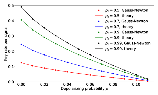
We compare results from instances for which there exist tight analytical key rate expressions to demonstrate that our Gauss-Newton method can achieve high accuracy with respect to the analytical key rates. There are known analytical expressions for entanglement-based BB84, prepare-and-measure BB84 as well as measurement-device-independent BB84 variants mentioned in Appendix C. We take the measurement-device-independent BB84 as an example since it involves the largest problem size among these three examples and therefore more numerically challenging. In Figure 5.1, we present instances with different choices of parameters for data generation. The instances are tested with a desktop computer that runs with the operating system Ubuntu 18.04.4 LTS, MATLAB version 2019a, Intel Xeon CPU E5-2630 v3 @ 2.40GHz 32 and 125.8 Gigabyte memory. We set the tolerance for the Gauss-Newton method.
In Figure 5.1, the numerical lower bounds from the Gauss-Newton method are close to the analytical results to at least 12 decimals and in many cases they agree up to 15 decimals.
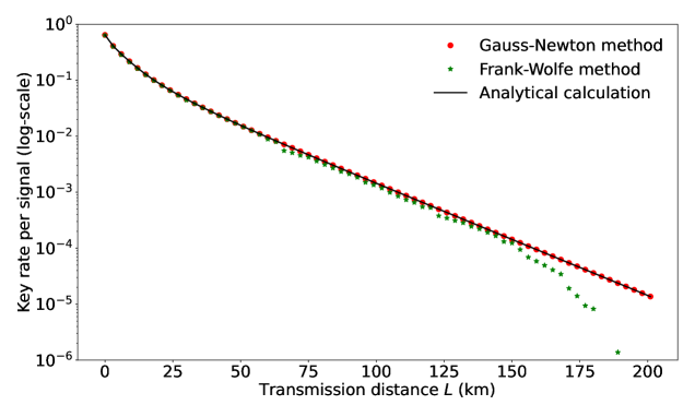
As noted in Section C.5, analytical results are also known when the channel noise parameter is set to zero since in this case, one may argue the optimal eavesdropping attack is the generalized beam splitting attack. This means the feasible set contains essentially a single up to unitaries. Since our objective function is unitarily invariant, one can analytically evaluate the key rate expression. In Figure 5.2, we compare the results from the Gauss-Newton method with the analytical key rate expressions for different choices of distances (See Section C.5 for the description about instances of this protocol example). These instances were run in the same machine as in Figure 5.1. We set the tolerance for the Gauss-Newton method.
5.2 Solving Numerically Challenging Instances
We show results where the Frank-Wolfe method without FR has difficulties in providing tight lower bounds in certain instances. In Figure 5.2, we plot results obtained previously in [26, Figure 2(b)] by the Frank-Wolfe method without FR. In particular, results from Frank-Wolfe method have visible differences from the analytical results starting from distance km. In addition the lower bounds are quite loose once the distance reaches km. In fact, there are points like the one around km where the Frank-Wolfe method cannot produce nontrivial (nonzero) lower bounds. On the other hand, the Gauss-Newton method provides much tighter lower bounds.
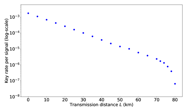
In Figure 5.3, we show another example to demonstrate the advantages of our method. These instances were run in the same machine as in Figure 5.2. For this discrete-phase-randomized BB84 protocol with discrete global phases (see Section C.6 for more descriptions), the previous Frank-Wolfe method was unable to find nontrivial lower bounds. This is because the previous method can only achieve an accuracy around for this problem due to the problem size. This is insufficient to produce nontrivial lower bounds for many instances since the key rates are on the order of or lower as shown in Figure 5.3. On the other hand, due to high accuracy of our method, we can obtain meaningful key rates. The advantage of high accuracy achieved by our method enables us to perform security analysis for protocols that involve previously numerically challenging problems. Like the discrete-phase-randomized BB84 protocol, these protocols involve more signal states, which lead to higher-dimensional problems.
5.3 Comparative Performance
In this section we examine the comparative performance among three algorithms; the Gauss-Newton method, the Frank-Wolfe method and cvxquad. The Gauss-Newton method refers to the algorithm developed throughout this paper. The Frank-Wolfe method refers to the algorithm developed in [5] and cvxquad is developed in [27]. We use Table 5.1 to present detailed reports on some selected instances. More numerics are reported throughout Tables C.1, C.2, C.3, C.4, C.5 and C.6 in Section C.7.
The instances are tested with MATLAB version 2021a using Dell PowerEdge R640 Two Intel Xeon Gold 6244 8-core 3.6 GHz (Cascade Lake) with 192 Gigabyte memory. For the instances corresponds to the DMCV protocol, we used the tolerance and the tolerance was used for the remaining instances. The maximum number of iteration was set to for the Gauss-Newton method.
| Problem Data | Gauss-Newton | Frank-Wolfe with FR | Frank-Wolfe w/o FR | cvxquad with FR | ||||||
|---|---|---|---|---|---|---|---|---|---|---|
| protocol | parameter | size | gap | time | gap | time | gap | time | gap | time |
| ebBB84 | (0.50,0.05) | (4,16) | 5.98e-13 | 0.40 | 1.01e-04 | 92.49 | 1.17e-04 | 93.05 | 5.46e-01 | 214.02 |
| ebBB84 | (0.90,0.07) | (4,16) | 1.42e-12 | 0.20 | 2.71e-04 | 91.26 | 2.75e-04 | 94.49 | 7.39e-01 | 177.64 |
| pmBB84 | (0.50,0.05) | (8,32) | 5.51e-13 | 0.23 | 1.12e-04 | 1.38 | 6.47e-04 | 1.91 | 5.26e-01 | 158.64 |
| pmBB84 | (0.90,0.07) | (8,32) | 5.13e-13 | 0.17 | 7.31e-05 | 1.29 | 6.25e-04 | 38.65 | 6.84e-01 | 233.43 |
| mdiBB84 | (0.50,0.05) | (48,96) | 1.14e-12 | 1.09 | 4.99e-05 | 104.31 | 5.22e-04 | 134.05 | 1.82e-01 | 557.08 |
| mdiBB84 | (0.90,0.07) | (48,96) | 2.96e-13 | 0.96 | 2.04e-04 | 106.61 | 2.85e-03 | 126.62 | 4.57e-01 | 537.52 |
| TFQKD | (0.80,100.00,0.70) | (12,24) | 1.15e-12 | 0.79 | 2.60e-09 | 1.21 | 1.57e-03 | 124.48 | n/a | 0.01 |
| TFQKD | (0.90,200.00,0.70) | (12,24) | 1.04e-12 | 0.44 | 3.98e-09 | 1.13 | 1.68e-04 | 2.25 | n/a | 0.00 |
| DMCV | (10.00,60.00,0.05,0.35) | (44,176) | 2.71e-09 | 507.83 | 4.35e-06 | 467.41 | 3.57e-06 | 657.08 | n/a | 0.01 |
| DMCV | (11.00,120.00,0.05,0.35) | (48,192) | 3.24e-09 | 700.46 | 2.35e-06 | 194.62 | 2.15e-06 | 283.06 | n/a | 0.01 |
| dprBB84 | (1.00,0.08,30.00) | (12,48) | 4.92e-13 | 1.19 | 3.85e-06 | 96.74 | 9.43e-05 | 141.38 | 118.81 | |
| dprBB84 | (2.00,0.14,30.00) | (24,96) | 1.04e-12 | 11.76 | 5.71e-06 | 17.66 | 5.38e-06 | 34.60 | 106.24 | |
| dprBB84 | (3.00,0.10,30.00) | (36,144) | 4.96e-13 | 63.26 | 6.48e-04 | 7.38 | 2.08e-02 | 29.00 | 582.64 | |
| dprBB84 | (4.00,0.12,30.00) | (48,192) | 3.80e-13 | 330.39 | 4.42e-05 | 13.78 | 9.79e-04 | 175.39 | 3303.23 | |
In Table 5.1 Problem Data refers to the data used to generate the instances. Gauss-Newton refers to the Gauss-Newton method. Frank-Wolfe refers to the Frank-Wolfe algorithm used in [5] and we use ‘with FR (w/o FR, resp)’ to indicate the model is solved with FR (without FR, resp). The header cvxquad with FR refers to the algorithm provided by [27] with FR reformulation. If a certain algorithm fails to give a reasonable answer within a reasonable amount of time, we give a ‘’ flag in the gap followed by the time taken to obtain the error message. We use ‘n/a’ to indicate the instances for which cvxquad is not applicable due to the size differences in the images under and due to FR.
The following provides details for the remaining headers in Table 5.1.
-
1.
protocol: the protocol name; refer to Appendix C;
-
2.
parameter: the parameters used for testing; see Section C.1 - Section C.6 for the ordering of the parameters;
-
3.
size: the size of original problem; are defined in (3.3);
-
4.
gap: the relative gap between the bestub and bestlb;
(5.1) -
5.
time: time taken in seconds.
We make some discussions on the formula 5.1. The best upper bound from Gauss-Newton algorithm is used for all instances for ‘bestub’ in 5.1. The Gauss-Newton algorithm computes the lower bounds as presented in Corollary 4.8. The Frank-Wolfe algorithm presented in [5] obtains the lower bound by a linearization technique near the optimal. As presented in [27], cvxquad uses the semidefinite approximations of the matrix logarithm. The lower bounds from cvxquad are often larger than the theoretical optimal values. This observation indicates that the lower bounds from cvxquad are not reliable. Therefore, we adopt the lower bound strategy used in [5] for cvxquad.
We now discuss the results in Table 5.1. Comparing the two columns gap and time among the different methods, we see that the Gauss-Newton method outperforms other algorithms in both the accuracy and the running time. For example, comparing Gauss-Newton and Frank-Wolfe with FR, the gaps and running times from Gauss-Newton are competitive. There are three instances that Gauss-Newton took longer time. We emphasize that the gap values with Gauss-Newton illustrate much higher accuracy.
We now illustrate that the reformulation strategy via FR contributes to superior algorithmic performances. For the columns Frank-Wolfe with FR and Frank-Wolfe w/o FR in Table 5.1, the FR reformulation contributes to not only giving tighter gaps but also reducing the running time significantly. We now consider the column corresponding to cvxquad with FR in Table 5.1. We see that the algorithm fails (marked with ‘’) with some instances due to the memory shortage. Facial reduction indeed contributes to the reduction on the problem sizes. For example, we reduced the problem sizes in Table 5.2.
| protocol | parameter | ||
|---|---|---|---|
| pmBB84 | |||
| mdiBB84 |
6 Conclusion
6.1 Summary
In this paper we have presented a robust numerical method for finding provable tight lower bounds for the convex optimization problem that finds the key rate for the QKD problem. Our empirical evidence illustrates consistent significant improvements in solution time and accuracy over previous methods. In particular, we solve many problems close to machine accuracy and provide theoretical provable accurate lower bounds. This includes previously unsolved problems. (See e.g., Table 5.1.)
This paper used novel convex optimization techniques applied specifically to the QKD problem. This includes reformulations of the convex optimization problem that finds the key rate. The result is a regularized problem that avoids the need for previously used perturbations and resulting possible instabilities. Below, we give a summary of the contributions for the model reformulation and for the algorithm.
6.1.1 Summary of the Model Reformulation
We have reformulated, simplified, and stabilized the model for QKD key rate calculation through the sequence
via (1) variable substitutions; (2) property of from Proposition 3.3; (3) facial reduction on ; (4) rotation of the constraints; (5) substituting the constraints back to the objective.
6.1.2 Summary of Algorithm 1
Our algorithm Algorithm 1 is based on a standard primal-dual interior-point approach applied to the FR stabilized model. However, it differs in several ways.
-
1.
We modify the primal feasibility to use a nullspace representation. Therefore, both primal and dual feasibility have a similar representation.
-
2.
We use a projected Gauss-Newton search direction to account for the overdetermined least squares problem arising from the optimality conditions. This means we project the Gauss-Newton direction after substituting using the primal-dual linear feasibility equations.
-
3.
We exploit the exact feasibility of linear constraints after a step length one for the Gauss-Newton method. Therefore, we attempt to take a primal and/or dual step length one as soon as possible. Exact feasibility results.
-
4.
We use a modified form of the dual to obtain a lower bound that is used along with an upper bound from the objective function to stop the algorithm when the duality gap is provably small. Our lower bound is a provably lower bound for the original problem as it is using a feasible dual point to evaluate the dual value. This is needed, as an approximate primal optimal value is not exactly optimal.
6.2 Future Plans
There are still many improvements that can be made. Exact primal feasibility was quickly obtained and maintained throughout the iterations. However, accurate dual feasibility was difficult to maintain. This is most likely due to the rounding errors in the numerical computation of the Hessian when is near the boundary of the positive semidefinite cone. This approximation can be improved by including a quasi-Newton approach, as we have accurate gradient evaluations. We maintain high accuracy results even in the cases where the Jacobian was not full rank at the optimum. This appears to be due to the special data structures and more theoretical analysis at the optimum can be done.
In this work, we considered a model with the linear constraints restricted to be equalities. While this model covers many interesting QKD protocols, there are scenarios where inequality constraints are needed, e.g., when using the flag-state squasher [7] to reduce the dimension. Moreover, there can be additional matrix inequality constraints when the dimension reduction method [8] is applied. It is interesting and important to address possible numerical instabilities introduced by those inequality constraints as was done in this paper.
Acknowledgements
We thank Kun Fang and Hamza Fawzi for discussions and Cunlu Zhou for kindly providing us the code presented in [10]. The authors H.H., J.I. and H.W. thank the support of the National Sciences and Engineering Research Council (NSERC) of Canada. Part of this work was done at the Institute for Quantum Computing, University of Waterloo, which is supported by Innovation, Science and Economic Development Canada. J.L. and N.L. are supported by NSERC under the Discovery Grants Program, Grant No. 341495, and also under the Collaborative Research and Development Program, Grant No. CRDP J 522308-17. Financial support for this work has been partially provided by Huawei Technologies Canada Co., Ltd.
Code Availability
The code developed in this work is currently available at this link.888https://www.math.uwaterloo.ca/~hwolkowi/henry/reports/ZGNQKDmainsolverUSEDforPUBLCNJuly31/ It will be integrated into the open-source QKD security software project, which can be accessed via the link.999https://openqkdsecurity.wordpress.com/
Appendix A Background Results and Proofs
A.1 Adjoints for Matrix Multiplication
Adjoints are essential for our interior point algorithm when using matrix-free methods. We define the symmetrization linear map, , as . The skew-symmetrization linear map, , is .
Lemma A.1 (adjoint of ).
Let be a given square complex matrix, and define the (left matrix multiplication) linear map by . Then the adjoint is defined by
| (A.1) |
If and , then the adjoint is defined by
| (A.2) |
Proof.
Lemma A.2 (adjoint of ).
Let be a given square complex matrix, and define the (right matrix multiplication) linear map by . Then the adjoint is defined by
| (A.5) |
If and , then the adjoint is defined by
| (A.6) |
Proof.
The proof is similar to the proof of Lemma A.1. ∎
A.2 Proof of Lemma 3.4
Proof.
Recall that
| (A.7) |
Let be a positive semidefinite matrix with rank and spectral decomposition
We only focus on the first term . Then
We note, from A.7, that
We also note that
Hence,
We now consider the first two terms in , . Similarly,
| (A.8) |
Then
This completes the proof (The induction steps are clear.). ∎
A.3 Derivatives for Quantum Relative Entropy under Positive Definite Assumptions
We can reformulate the quantum relative entropy function defined in the key rate optimization 2.2 as
| (A.9) |
Here, the linear map is added to the second term in A.9 above, and the equality follows from Proposition 3.3.
In this section, we review the gradient (Fréchet derivative), and the image of the Hessian, for the reformulated relative entropy function defined in A.9. We obtain the derivatives of under the assumption that the matrix-log is acting on positive definite matrices. This assumption is needed for differentiability. Note that the difficulty arising from the singularity is handled by using perturbations in [5, 10]. This emphasizes the need for the regularization below as otherwise in A.9 is never differentiable. We avoid using perturbations in this paper by applying FR in the sections below.
We now use the chain rule and derive the first and the second order derivatives of the composition of a linear and entropy function.
Lemma A.3.
Let be a linear map that preserves positive semidefiniteness. Assume that . Define the composite function by
Then the gradient of at is
and the Hessian of at acting on is
where denotes the Fréchet derivative.
Proof.
We first work on the first-order derivative.
| (A.10) | ||||
Note that we used the fact that the directional derivative of matrix-log at in the direction is:
Similarly, the Hessian at acting on can be obtained as follows.
| (A.11) |
∎
Under the assumption that , we can use Lemma 3.4 and show that . Using Lemma A.3 and (3.5), we obtain the first and the second order derivatives of the objective function in (A.9).
Corollary A.4.
Suppose that and . Then the gradient of at is
| (A.12) |
The Hessian at acting on the direction is
| (A.13) |
A.4 Proof of Theorem 3.6
Proof.
We provide an alternative, self-contained proof. We note that the key is finding an exposing vector for , i.e., such that , . See e.g., [13]. The standard theorem of the alternative for strict feasibility, Lemma 2.4, yields the following equalities for :
It is equivalent to look at the smaller problem and find so that
Since the reduced density operator constraint requires that , we get
i.e., the exposing vector , for some . Conversely, we can set , by the basis property of the , i.e., the basis property means we can always find an appropriate so that . We get that . Therefore, , with , is an exposing vector as desired, i.e., we have
Thus we get the conclusion that , as desired. ∎
A.5 Proof of Theorem 4.1
Proof.
The dual in Item 2 is obtained from from standard min-max argument; See [28, Chapter 5].
That strong duality holds comes from our regularization process, i.e., the existence of a Slater point; see [29, Chapter 8].
Item 3 is the standard optimality conditions for convex programming, where the dual feasibility holds from Theorem 3.14. ∎
Appendix B Implementation Details
In this section we look at simplifications for evaluations of the objective function and its derivatives.
B.1 Matrix Representations of Derivatives
We now include a matrix representation for the derivatives.
Let be given compatible matrices. If is Hermitian, then the linear system can be written as
Note that is the transpose of , i.e., without conjugation.
Let be a continuously differentiable function. The first divided difference of at is defined as
| (B.1) |
If is a diagonal matrix with diagonal entries , then we define to be the symmetric matrix given by .
Lemma B.1.
Let be a linear map, , and . Let be the spectral decomposition of at , and the Hessian of at in the direction are given by
and
where is the first divided difference of the logarithm function , see B.1 and the paragraph below.
In the actual computation, it is more convenient to express the gradient and Hessian in matrix form. Let be the matrix representation of . The Hessian in matrix form is
B.2 Matrix Representation of the Second Projected Gauss-Newton System
We present the matrix representation of 4.6. Let be a basis element of . Then has the representation . Then the LHS of 4.6 becomes
| (B.2) |
Applying 101010The operator vec maps a real matrix to a column vector by stacking the columns on top of one another. is a generalization of vec for complex matrices. It maps a complex matrix to the column vector . to the terms related to , we have the following matrix representation:
Similarly, applying on the terms related to , we have the following matrix representation:
The RHS of 4.6 becomes . Thus, is obtained be solving the system
B.3 Implementation Heuristics
We now discuss the implementation details. This involves preprocessing for a nullspace representation and preconditioning. The details follow.
B.3.1 Stopping Criteria
We terminate the algorithm when the optimality condition (4.3) is approximately satisfied. Denote the residual in Theorem 4.5 by
and the denominator term by
Then
| (B.3) |
In other words, for a pre-defined tolerance , we terminate the algorithm when the relstopgap. If the algorithm computes lower and upper bounds of the optimal value throughout its execution, we may terminate the algorithm when the gap between lower and upper bounds is within . Finally, a common way to terminate an algorithm is to impose restrictions on the running time, e.g., setting an upper bound on the number of iterations or the physical running time.
B.3.2 GN Direction using Sparse Nullspace Representation
We let , and construct a matrix representation for the Hessian, and a matrix representation for the linear constraints that includes a permutation of rows and columns with inverse column permutation , so that
We can ignore the row permutations. We have
We now get the nullspace representation:
| (B.4) |
The permutation of rows and columns are done in order to obtain a simple, near triangular, well conditioned so that can be done simply and maintain sparsity if possible. The permutation of the rows does not affect the problem and we can ignore it. However the permutation of the columns cannot be ignored. We get the following
By abuse of notation, the Gauss-Newton direction can now be found from:
| (B.5) |
B.3.3 Preconditioning
The overdetermined linear system in B.5 can be ill-conditioned. We use diagonal preconditioning, i.e., we let , for unit vectors and then column precondition using
This diagonal preconditioning has been shown to be the optimal diagonal preconditioning for the so-called -condition number, [30]. It performs exceptionally well in our tests below.
B.3.4 Step Lengths
The GN method is based on a linearization that suggests a step length of one. However, long step methods are known to be more efficient in practice for interior point methods for linear SDPs. Typically step lengths are found using backtracking to ensure primal-dual positive definiteness of .
In our case we do not have a linear objective and we typically experience Maratos type situations, i.e., we get fast convergence for primal feasibility but slow and no convergence for dual feasibility. However, we do have the gradient and Hessian of the objective function and therefore can minimize the quadratic model for the objective function in the search direction
Therefore, we begin the backtracking with this step.
Moreover, we take a step length of one as soon as possible, and only after this do we allow step lengths larger than one. This means that exact primal feasibility holds for all further steps. This happens relatively early for our numerical tests.
Appendix C Descriptions and Further Numerics of the Protocols
We briefly describe six QKD protocols where we compare our algorithm to other algorithms. We also describe how the data ( in 2.2) is generated. In addition, we remark on the level of numerical difficulty for each example. We consider four variants of the Bennett-Brassard 1984 (BB84) protocol [3] including single-photon based variants: entanglement-based (Section C.1), prepare-and-measure (Section C.2), measurement-device-independent [31] (Section C.3) and a coherent-state based variant with discrete global phase randomization [32] (Section C.6). We also consider the single-photon version of the twin-field QKD [33] (Section C.4). Another interesting protocol in our numerical tests is the quadrature phase-shift keying scheme of discrete-modulated continuous-variable QKD with heterodyne detection (Section C.5), see [26, Protocol 2]. These protocols correspond to numerical problems with the level of difficulty ranging from easy to difficult. In the descriptions below, we use the Dirac notation for quantum states which are vectors in the underlying Hilbert space. We skip the description about some common classical postprocessing steps in a QKD protocol like error correction and privacy amplification since they are unimportant for our discussions here. We note that the description of linear maps and directly follow from the protocol description by following the simplification procedure explained in [26, Appendix A]. We omit those detailed descriptions here and note that the explicit expressions for some of protocols can also be found in [6, Appendix D].
C.1 Entanglement-Based BB84
We consider this protocol with a single-photon source and restrict our discussions to the qubit space. In the quantum communication phase, Alice and Bob each receive one half of a bipartite state. This is supposed to be a two-qubit maximally entangled state before Eve’s tampering. And the measure in the basis is with probability , or in basis with a probability . In the classical communication phase, they announce their basis choices for each round and perform sifting to keep those rounds where they both chose the same basis. In the end, they generate keys from both and bases.
In the simulation, we assume both bases have the same error rate . In particular, (in 2.2) contains the -basis error rate, -basis error rate constraints as well as one coarse-grained constraint for each mismatched basis choice scenario. This is to ensure that Alice and Bob get completely uncorrelated outcomes in that case. In other words, the data are determined by . This test example is supposed to be numerically easy, since it involves the smallest possible size of for QKD, i.e., four. Moreover, there is no reduced density operator constraint for this example. In Table 5.1, instances of this test example are labeled as ebBB84() for different values of and .
C.2 Prepare-and-Measure BB84
Another protocol example in our numerical tests is the prepare-and-measure version of BB84 with a single-photon source. In the quantum communication phase, Alice chooses the basis with a probability or the basis with a probability . When she chooses the basis, she sends either or at random, where and are eigenstates of the Pauli operator. When she chooses the basis, she sends either or at random, where . After Alice sends the state of her choice to Bob, Bob chooses to measure in the basis with a probability or the basis with a probability . The rest of the protocol is exactly the same as the entanglement-based BB84 protocol described in Section C.1. We call as stated in BB84.
For the security analysis, we use the source-replacement scheme [16] to convert it to its equivalent entanglement-based scheme. Therefore, the main differences between this example and the one in Section C.1 are: (1) the dimension of Alice’s system for this example is four due to the source-replacement scheme, while it is two for the entanglement-based BB84; (2) there is the reduced density operator constraint which is of size and translated to linear constraints. In this test example, the size of is and the size of is before FR.
The data simulation is done in a similar way as that in the entanglement-based BB84 protocol, i.e., . In Table 5.1, instances of this test example are labeled as pmBB84().
C.3 Measurement-Device-Independent BB84
In the measurement-device-independent variant of BB84 with single-photon sources, Alice and Bob each prepare one of four BB84 states (with the probability of choosing the basis as ). Then they both send this to an untrusted third-party Charlie for measurements. He ideally then performs the Bell-state measurements and announces the outcomes. We consider a setup where Charlie only uses linear optics, and thus can only measure two out of four Bell states. In this protocol, Charlie announces either a successful Bell-state measurement or a failure. If a successful measurement, Charlie then also announces the Bell state. Therefore, there are three possible announcement outcomes. After the announcement, Alice and Bob perform the basis sifting, as well as discard rounds that are linked to unsuccessful events. They then generate keys from rounds where they both chose the basis and Charlie’s announcement is one of the successful events.
We now consider the measurement-device-independent type of protocols. As described in [4], the optimization variable involves three parties as . Here, registers together serve the role of in the reduced density operator constraint set 2.5. The dimension of Alice’s system is and so is Bob’s dimension. The register is a classical register that stores the announcement outcome. Thus it is three-dimensional with three possible announcement outcomes. In the data simulation, we assume that each qubit sent to Charlie goes through a depolarizing channel, with the depolarizing probability .
In the numerical tests, we label instances of this protocol example as mdiBB84(). The size of is and that of is before FR.
C.4 Twin-Field QKD
As above, this protocol also uses the measurement-device-independent setup. The exact protocol description can be found in [34, Protocol 1]. In this protocol, Alice and Bob each prepare a state () with , where the register is a qubit system and the register is an optical mode with the vacuum state and the single-photon state . After they send states to the intermediate station, Charlie at the intermediate station is supposed to perform the single-photon interference of these two signal pulses and then announces the measurement outcome for each of two detectors: click or no-click. Then Alice and Bob each perform the -basis measurement on their local qubits with a probability or the -basis measurement with a probability . They generate keys from rounds where they both choose the basis and where Charlie announces a successful measurement outcome, that is, having exactly one of two detectors click.
In the simulation, we consider a lossy channel, with the transmittance , for the distance in kilometers between Alice and Bob. We consider the symmetric scenario where Charlie is at an equal distance away from Alice and Bob. We also consider detector imperfections: each detector at Charlie’s side has detector efficiency and dark count probability . In instances of this protocol, data is generated as a function of: that appears in the states and ; the total distance in kilometers between Alice and Bob; and the probability of choosing basis . The instances of this test example are labeled as TFQKD().
C.5 Discrete-Modulated Continuous-Variable QKD
The exact protocol description can be found in [26, Protocol 2]. We use the same simulation method described in [26, Equation (30)] to generate the data . In this protocol, Alice sends Bob one of four coherent states , where for . And Bob performs the heterodyne measurement, i.e., measuring both - and -quadratures after splitting the signal into two halves by a beamsplitter. The first and second moments of - and -quadratures are used to constrain . The data simulation uses a phase-invariant Gaussian channel with transmittance and excess noise to generate those values. We use the same photon-number cutoff assumption used there to truncate the infinite-dimensional Hilbert space. For the calculation, it is typically sufficient to choose to minimize the effects of errors due to the truncation. For simplicity, we assume the detector at Bob’s side is an ideal detector. The channel transmittance, , is related to the transmission distance between Alice and Bob, by .
Let be an integer that represents the cutoff photon number. Before FR, the sizes of and are and , respectively. In Table 5.1, we label instances of this example as DMCV().
When the noise , this problem can be solved analytically via physical arguments. The detailed instructions for analytical calculation can be found in [26, Appendix C]. We use this special case to demonstrate that our interior-point method can reproduce the analytical results to high precision.
C.6 Discrete-Phase-Randomized BB84
We consider the phase-encoding BB84 protocol with (a parameter) discrete global phases evenly spaced between [0, ] [32]. A detailed protocol description can also be found in [6, Sec. IV D]. In particular, each of four BB84 states is realized by a two-mode coherent state , where the first mode is the phase reference mode and the second mode encodes the private information. In particular, the is a global phase that involves discrete phase randomization, i.e., . The relative phase for encoding is , where correspond to the basis and correspond to the basis.
Data simulation is done in exactly the same way as in [6, Section IV D], where we consider detector imperfections and a lossy channel with a misalignment error due to phase drift.
We remark that the instances of this test example become more challenging as one increases the number of discrete phases , since the size of is and the size of is before FR. In all instances of this protocol, we choose and the data are simulated with detector efficiency , dark count probability and relative phase drift of . The final key rate values are presented by taking the error correction efficiency as 1.16. In the numerical tests, we label instances of this protocol as dprBB84().
C.7 Additional Numerical Results
| Problem Data | Gauss-Newton | Frank-Wolfe with FR | Frank-Wolfe w/o FR | cvxquad with FR | ||||||
|---|---|---|---|---|---|---|---|---|---|---|
| protocol | parameter | size | gap | time | gap | time | gap | time | gap | time |
| ebBB84 | (0.50,0.01) | (4,16) | 1.14e-12 | 0.42 | 5.96e-05 | 95.32 | 5.88e-05 | 99.09 | 6.37e-01 | 216.75 |
| ebBB84 | (0.50,0.03) | (4,16) | 8.35e-13 | 0.20 | 6.37e-05 | 93.35 | 6.24e-05 | 99.47 | 5.88e-01 | 258.98 |
| ebBB84 | (0.50,0.05) | (4,16) | 5.98e-13 | 0.18 | 1.01e-04 | 95.31 | 1.17e-04 | 101.36 | 5.46e-01 | 213.04 |
| ebBB84 | (0.50,0.07) | (4,16) | 1.05e-12 | 0.19 | 1.66e-04 | 96.92 | 1.65e-04 | 100.46 | 5.07e-01 | 179.38 |
| ebBB84 | (0.50,0.09) | (4,16) | 1.35e-12 | 0.18 | 1.43e-04 | 96.35 | 2.55e-04 | 100.64 | 4.70e-01 | 170.14 |
| ebBB84 | (0.70,0.01) | (4,16) | 1.21e-13 | 0.21 | 7.60e-05 | 96.33 | 7.62e-05 | 99.14 | 7.06e-01 | 172.09 |
| ebBB84 | (0.70,0.03) | (4,16) | 6.36e-13 | 0.18 | 9.16e-05 | 96.77 | 9.15e-05 | 99.78 | 6.59e-01 | 160.88 |
| ebBB84 | (0.70,0.05) | (4,16) | 5.34e-13 | 0.18 | 1.67e-04 | 97.03 | 1.03e-04 | 100.73 | 6.14e-01 | 173.77 |
| ebBB84 | (0.70,0.07) | (4,16) | 1.26e-12 | 0.20 | 1.80e-04 | 96.22 | 1.74e-04 | 100.71 | 5.70e-01 | 261.77 |
| ebBB84 | (0.70,0.09) | (4,16) | 2.06e-13 | 0.18 | 3.85e-04 | 97.08 | 2.61e-04 | 101.55 | 5.26e-01 | 225.94 |
| ebBB84 | (0.90,0.01) | (4,16) | 5.40e-13 | 0.17 | 1.02e-04 | 97.68 | 1.03e-04 | 98.45 | 8.73e-01 | 141.93 |
| ebBB84 | (0.90,0.03) | (4,16) | 7.05e-13 | 0.21 | 1.25e-04 | 97.97 | 1.43e-04 | 99.50 | 8.27e-01 | 164.26 |
| ebBB84 | (0.90,0.05) | (4,16) | 3.48e-13 | 0.18 | 1.48e-04 | 96.91 | 9.81e-05 | 100.99 | 7.83e-01 | 186.87 |
| ebBB84 | (0.90,0.07) | (4,16) | 1.42e-12 | 0.17 | 2.71e-04 | 96.55 | 2.75e-04 | 101.79 | 7.39e-01 | 179.55 |
| ebBB84 | (0.90,0.09) | (4,16) | 1.09e-12 | 0.21 | 3.51e-04 | 96.40 | 3.42e-04 | 101.99 | 6.94e-01 | 228.63 |
| Problem Data | Gauss-Newton | Frank-Wolfe with FR | Frank-Wolfe w/o FR | cvxquad with FR | ||||||
|---|---|---|---|---|---|---|---|---|---|---|
| protocol | parameter | size | gap | time | gap | time | gap | time | gap | time |
| pmBB84 | (0.50,0.01) | (8,32) | 5.96e-13 | 0.38 | 6.19e-06 | 1.95 | 4.64e-04 | 25.18 | 6.30e-01 | 190.28 |
| pmBB84 | (0.50,0.03) | (8,32) | 1.01e-12 | 0.18 | 1.71e-05 | 1.37 | 6.54e-04 | 90.80 | 5.74e-01 | 181.83 |
| pmBB84 | (0.50,0.05) | (8,32) | 5.51e-13 | 0.19 | 1.12e-04 | 1.31 | 6.47e-04 | 1.94 | 5.26e-01 | 159.28 |
| pmBB84 | (0.50,0.07) | (8,32) | 8.88e-14 | 0.16 | 5.89e-05 | 1.30 | 8.77e-04 | 1.98 | 4.81e-01 | 161.49 |
| pmBB84 | (0.50,0.09) | (8,32) | 9.38e-13 | 0.19 | 6.71e-05 | 1.42 | 9.04e-04 | 2.03 | 4.40e-01 | 179.01 |
| pmBB84 | (0.70,0.01) | (8,32) | 7.69e-13 | 0.25 | 7.62e-06 | 1.33 | 2.39e-04 | 130.73 | 7.03e-01 | 213.43 |
| pmBB84 | (0.70,0.03) | (8,32) | 4.75e-13 | 0.18 | 2.38e-05 | 1.32 | 2.68e-04 | 133.52 | 6.51e-01 | 246.50 |
| pmBB84 | (0.70,0.05) | (8,32) | 6.16e-13 | 0.17 | 3.52e-05 | 1.37 | 3.37e-04 | 134.59 | 6.04e-01 | 281.84 |
| pmBB84 | (0.70,0.07) | (8,32) | 6.30e-13 | 0.19 | 7.43e-05 | 1.26 | 3.04e-04 | 141.97 | 5.60e-01 | 259.33 |
| pmBB84 | (0.70,0.09) | (8,32) | 8.47e-13 | 0.16 | 9.25e-05 | 1.29 | 3.55e-04 | 7.07 | 5.18e-01 | 297.32 |
| pmBB84 | (0.90,0.01) | (8,32) | 3.68e-13 | 0.18 | 7.07e-06 | 1.33 | 3.27e-04 | 4.98 | 8.60e-01 | 247.82 |
| pmBB84 | (0.90,0.03) | (8,32) | 1.27e-12 | 0.18 | 2.29e-05 | 1.35 | 5.43e-04 | 137.74 | 7.96e-01 | 230.35 |
| pmBB84 | (0.90,0.05) | (8,32) | 1.36e-12 | 0.16 | 4.62e-05 | 1.35 | 5.96e-04 | 72.04 | 7.38e-01 | 291.83 |
| pmBB84 | (0.90,0.07) | (8,32) | 5.13e-13 | 0.17 | 7.31e-05 | 1.35 | 6.25e-04 | 40.11 | 6.84e-01 | 235.27 |
| pmBB84 | (0.90,0.09) | (8,32) | 7.84e-13 | 0.19 | 1.06e-04 | 1.32 | 7.39e-04 | 142.32 | 6.32e-01 | 244.81 |
| Problem Data | Gauss-Newton | Frank-Wolfe with FR | Frank-Wolfe w/o FR | cvxquad with FR | ||||||
|---|---|---|---|---|---|---|---|---|---|---|
| protocol | parameter | size | gap | time | gap | time | gap | time | gap | time |
| mdiBB84 | (0.50,0.01) | (48,96) | 1.25e-12 | 1.27 | 1.64e-05 | 109.60 | 3.75e-04 | 498.82 | 2.11e-01 | 719.99 |
| mdiBB84 | (0.50,0.03) | (48,96) | 8.37e-13 | 0.81 | 3.53e-05 | 107.90 | 5.31e-04 | 2811.15 | 1.95e-01 | 630.89 |
| mdiBB84 | (0.50,0.05) | (48,96) | 1.14e-12 | 0.83 | 4.99e-05 | 111.08 | 5.22e-04 | 464.06 | 1.82e-01 | 586.22 |
| mdiBB84 | (0.50,0.07) | (48,96) | 1.35e-12 | 1.08 | 4.87e-05 | 335.57 | 4.60e-04 | 2169.93 | 1.71e-01 | 569.14 |
| mdiBB84 | (0.50,0.09) | (48,96) | 1.25e-12 | 0.91 | 8.27e-05 | 342.04 | 4.37e-04 | 829.61 | 1.60e-01 | 568.97 |
| mdiBB84 | (0.70,0.01) | (48,96) | 1.20e-12 | 0.68 | 2.20e-05 | 5.68 | 5.53e-04 | 901.29 | 3.79e-01 | 719.27 |
| mdiBB84 | (0.70,0.03) | (48,96) | 4.24e-13 | 1.05 | 1.11e-04 | 5.83 | 1.21e-03 | 256.79 | 3.55e-01 | 670.49 |
| mdiBB84 | (0.70,0.05) | (48,96) | 1.06e-12 | 1.10 | 6.92e-05 | 340.21 | 1.75e-03 | 865.68 | 3.31e-01 | 651.44 |
| mdiBB84 | (0.70,0.07) | (48,96) | 5.71e-13 | 0.95 | 1.37e-04 | 337.17 | 1.55e-03 | 864.25 | 3.09e-01 | 604.94 |
| mdiBB84 | (0.70,0.09) | (48,96) | 1.57e-13 | 0.92 | 1.61e-04 | 347.21 | 2.24e-03 | 872.37 | 2.88e-01 | 604.71 |
| mdiBB84 | (0.90,0.01) | (48,96) | 8.44e-13 | 0.66 | 4.42e-05 | 343.38 | 3.21e-03 | 175.20 | 5.53e-01 | 710.65 |
| mdiBB84 | (0.90,0.03) | (48,96) | 1.39e-12 | 0.90 | 9.15e-05 | 343.08 | 3.66e-03 | 301.29 | 5.16e-01 | 671.95 |
| mdiBB84 | (0.90,0.05) | (48,96) | 9.88e-13 | 0.84 | 1.73e-04 | 345.79 | 4.64e-03 | 519.80 | 4.85e-01 | 644.23 |
| mdiBB84 | (0.90,0.07) | (48,96) | 2.96e-13 | 1.05 | 2.04e-04 | 338.15 | 2.85e-03 | 148.24 | 4.57e-01 | 580.20 |
| mdiBB84 | (0.90,0.09) | (48,96) | 5.21e-13 | 1.02 | 2.52e-04 | 343.95 | 3.26e-03 | 193.04 | 4.31e-01 | 595.07 |
| Problem Data | Gauss-Newton | Frank-Wolfe with FR | Frank-Wolfe without FR | |||||
|---|---|---|---|---|---|---|---|---|
| protocol | parameter | size | gap | time | gap | time | gap | time |
| TFQKD | (0.75,50.00,0.70) | (12,24) | 8.45e-13 | 1.33 | 2.72e-09 | 2.04 | 1.83e-03 | 155.08 |
| TFQKD | (0.75,100.00,0.70) | (12,24) | 1.42e-12 | 0.86 | 3.75e-09 | 1.35 | 1.53e-03 | 153.57 |
| TFQKD | (0.75,150.00,0.70) | (12,24) | 9.94e-13 | 0.78 | 2.82e-09 | 1.39 | 7.82e-04 | 162.13 |
| TFQKD | (0.75,200.00,0.70) | (12,24) | 1.15e-12 | 1.02 | 3.98e-09 | 1.37 | 7.19e-04 | 155.11 |
| TFQKD | (0.75,250.00,0.70) | (12,24) | 6.79e-13 | 0.79 | 8.21e-09 | 1.32 | 3.14e-04 | 172.53 |
| TFQKD | (0.80,50.00,0.70) | (12,24) | 1.15e-12 | 0.77 | 2.82e-09 | 1.39 | 1.52e-03 | 156.17 |
| TFQKD | (0.80,100.00,0.70) | (12,24) | 1.15e-12 | 1.08 | 2.60e-09 | 1.33 | 1.57e-03 | 156.11 |
| TFQKD | (0.80,150.00,0.70) | (12,24) | 1.25e-12 | 0.94 | 2.97e-09 | 1.29 | 8.30e-04 | 158.12 |
| TFQKD | (0.80,200.00,0.70) | (12,24) | 9.23e-13 | 0.73 | 4.23e-09 | 1.32 | 5.60e-04 | 155.45 |
| TFQKD | (0.80,250.00,0.70) | (12,24) | 3.91e-13 | 0.55 | 2.22e-09 | 1.35 | 1.97e-04 | 164.83 |
| TFQKD | (0.90,50.00,0.70) | (12,24) | 8.08e-13 | 0.79 | 4.30e-09 | 1.30 | 1.55e-03 | 156.38 |
| TFQKD | (0.90,100.00,0.70) | (12,24) | 1.38e-12 | 0.37 | 3.62e-09 | 1.31 | 1.23e-03 | 154.08 |
| TFQKD | (0.90,150.00,0.70) | (12,24) | 1.14e-12 | 0.61 | 2.87e-09 | 1.28 | 6.02e-04 | 161.73 |
| TFQKD | (0.90,200.00,0.70) | (12,24) | 1.04e-12 | 0.34 | 3.98e-09 | 1.36 | 1.68e-04 | 2.63 |
| TFQKD | (0.90,250.00,0.70) | (12,24) | 5.77e-13 | 0.43 | 2.77e-09 | 1.37 | 1.08e-05 | 2.07 |
| TFQKD | (0.95,50.00,0.70) | (12,24) | 9.84e-13 | 0.77 | 4.00e-09 | 1.43 | 1.38e-03 | 156.09 |
| TFQKD | (0.95,100.00,0.70) | (12,24) | 1.06e-12 | 0.70 | 4.36e-09 | 1.41 | 7.47e-04 | 153.19 |
| TFQKD | (0.95,150.00,0.70) | (12,24) | 1.36e-12 | 0.71 | 3.92e-09 | 1.35 | 8.38e-04 | 149.27 |
| TFQKD | (0.95,200.00,0.70) | (12,24) | 7.63e-13 | 0.65 | 2.60e-09 | 1.36 | 3.13e-04 | 150.75 |
| TFQKD | (0.95,250.00,0.70) | (12,24) | 1.02e-12 | 0.64 | 3.61e-09 | 1.42 | 5.56e-06 | 1.81 |
| Problem Data | Gauss-Newton | Frank-Wolfe with FR | Frank-Wolfe without FR | |||||
|---|---|---|---|---|---|---|---|---|
| protocol | parameter | size | gap | time | gap | time | gap | time |
| DMCV | (10.00,60.00,0.05,0.35) | (44,176) | 2.71e-09 | 1016.19 | 4.35e-06 | 612.62 | 3.57e-06 | 919.84 |
| DMCV | (10.00,120.00,0.05,0.35) | (44,176) | 2.70e-09 | 1090.41 | 2.27e-06 | 216.61 | 2.16e-06 | 277.47 |
| DMCV | (10.00,180.00,0.05,0.35) | (44,176) | 2.87e-09 | 1173.14 | 1.90e-07 | 23.64 | 1.36e-07 | 32.50 |
| DMCV | (11.00,60.00,0.05,0.35) | (48,192) | 3.05e-09 | 1419.71 | 2.50e-06 | 768.52 | 1.43e-06 | 1095.78 |
| DMCV | (11.00,120.00,0.05,0.35) | (48,192) | 3.24e-09 | 1484.12 | 2.35e-06 | 261.89 | 2.15e-06 | 380.63 |
| DMCV | (11.00,180.00,0.05,0.35) | (48,192) | 3.40e-09 | 1796.16 | 2.53e-07 | 26.98 | 1.59e-07 | 38.62 |
| DMCV | (10.00,150.00,0.02,0.70) | (44,176) | 2.07e-09 | 1143.23 | 1.67e-06 | 83.32 | 1.82e-06 | 99.96 |
| DMCV | (10.00,200.00,0.02,0.70) | (44,176) | 1.96e-09 | 1214.62 | 7.29e-07 | 21.26 | 7.06e-07 | 28.04 |
| DMCV | (10.00,150.00,0.02,0.80) | (44,176) | 3.27e-09 | 1113.17 | 1.10e-06 | 105.03 | 1.85e-06 | 106.68 |
| DMCV | (10.00,200.00,0.02,0.80) | (44,176) | 1.63e-09 | 1106.38 | 3.18e-07 | 19.61 | 2.90e-07 | 26.11 |
| DMCV | (11.00,150.00,0.02,0.70) | (48,192) | 3.31e-09 | 1607.78 | 1.72e-06 | 103.49 | 1.36e-06 | 150.76 |
| DMCV | (11.00,200.00,0.02,0.70) | (48,192) | 3.05e-09 | 1573.12 | 7.12e-07 | 27.40 | 6.68e-07 | 35.62 |
| DMCV | (11.00,150.00,0.02,0.80) | (48,192) | 3.37e-09 | 1597.15 | 1.36e-06 | 93.86 | 1.57e-06 | 115.21 |
| DMCV | (11.00,200.00,0.02,0.80) | (48,192) | 3.38e-09 | 1541.27 | 3.38e-07 | 25.34 | 2.99e-07 | 34.36 |
| Problem Data | Gauss-Newton | Frank-Wolfe with FR | Frank-Wolfe without FR | |||||
|---|---|---|---|---|---|---|---|---|
| protocol | parameter | size | gap | time | gap | time | gap | time |
| dprBB84 | (1.00,0.08,15.00) | (12,48) | 9.42e-13 | 1.66 | 3.85e-06 | 117.56 | 1.03e-04 | 189.23 |
| dprBB84 | (1.00,0.08,30.00) | (12,48) | 4.92e-13 | 1.70 | 3.85e-06 | 114.97 | 9.43e-05 | 178.82 |
| dprBB84 | (1.00,0.14,15.00) | (12,48) | 2.96e-13 | 0.91 | 3.63e-04 | 115.55 | 1.16e-02 | 178.91 |
| dprBB84 | (1.00,0.14,30.00) | (12,48) | 5.21e-13 | 1.43 | 2.60e-04 | 1.89 | 8.31e-03 | 2.51 |
| dprBB84 | (2.00,0.08,15.00) | (24,96) | 1.10e-12 | 22.06 | 9.58e-05 | 41.11 | 2.11e-03 | 82.96 |
| dprBB84 | (2.00,0.08,30.00) | (24,96) | 9.58e-13 | 22.26 | 1.17e-04 | 26.10 | 7.32e-06 | 114.66 |
| dprBB84 | (2.00,0.14,15.00) | (24,96) | 1.35e-12 | 24.93 | 1.89e-05 | 7.56 | 5.11e-04 | 16.59 |
| dprBB84 | (2.00,0.14,30.00) | (24,96) | 1.04e-12 | 24.63 | 5.71e-06 | 20.79 | 5.38e-06 | 42.06 |
| dprBB84 | (2.00,0.14,30.00) | (24,96) | 1.04e-12 | 24.82 | 5.71e-06 | 20.19 | 5.38e-06 | 44.72 |
| dprBB84 | (3.00,0.08,15.00) | (36,144) | 1.38e-12 | 129.39 | 2.36e-04 | 12.94 | 7.41e-03 | 33.59 |
| dprBB84 | (3.00,0.08,30.00) | (36,144) | 6.33e-13 | 139.34 | 2.26e-04 | 12.54 | 7.04e-03 | 36.53 |
| dprBB84 | (3.00,0.14,15.00) | (36,144) | 1.30e-12 | 118.84 | 4.32e-05 | 41.49 | 1.43e-04 | 50.07 |
| dprBB84 | (3.00,0.14,30.00) | (36,144) | 3.32e-13 | 127.94 | 5.80e-06 | 11.32 | 5.74e-06 | 37.63 |
| dprBB84 | (4.00,0.08,15.00) | (48,192) | 6.98e-09 | 766.17 | 2.88e-04 | 61.19 | 8.10e-03 | 235.02 |
| dprBB84 | (4.00,0.08,30.00) | (48,192) | 2.13e-09 | 786.01 | 2.97e-04 | 21.23 | 8.45e-03 | 232.35 |
| dprBB84 | (4.00,0.14,15.00) | (48,192) | 2.85e-12 | 539.08 | 1.29e-04 | 18.50 | 3.85e-03 | 201.96 |
| dprBB84 | (4.00,0.14,30.00) | (48,192) | 1.17e-12 | 545.04 | 1.26e-04 | 25.67 | 3.73e-03 | 209.05 |
We remark on the behavior of the Frank-Wolfe method when used without FR. Table 5.1 shows that two instances of the TFQKD protocol have vastly different running times. Similar situations without FR also occur in the tables presented here. The Frank-Wolfe method that is used and described in [5] adopts a two-step procedure. The running time of this method is mainly dependent on the number of iterations, since each iteration solves a linear SDP problem using CVX. There are two stopping conditions: the first depends on the value of the gradient information; the second is the maximum number of iterations, currently set at . For the instances with short running time, termination typically occurred due to the gradient condition; the other instances stopped after reaching the maximum number of iterations. A likely reason for early termination is the perturbation approach used to preserve positive definiteness of the matrices involved in the objective function. We emphasize that early termination still leads to reliable (but pessimistically lower) key rates. More explanations can be found in [5]. As discussed in this paper, a general motivation for FR is to avoid numerical instability associated with such perturbation approaches, i.e., without FR, we typically have the erratic behavior due to ill-posedness of the problems.
Index
- , line segment §2.5
- §3.3
- §3.3
- , Frobenius norm §2.3
- , Kronecker product §2.1
- §2.5, §2.5
- , conjugate transpose §2.3
- §2.1, §3.2.1
- adjoint §2.4
- adjoint of , §2.4
- algorithm, GN interior point for QKD §4.4
- §2.2
- , block diagonal matrix with diagonal blocks §2.2
- compact spectral decomposition §2.5, §3.2.2
- conjugate transpose, §2.3
- constraint sets §2.1
- convex cone §2.5
- density matrices §2.1
- , GN -direction §4.2, §4.3.1
- dual cone §2.5
- dual cone, §2.5
- exposing vector §A.4, §2.5, §3.2.2
- §2.1
- face Definition 2.1
- , minimal face §2.5
- facially reduced reduced density operator constraint §3.2.1
- Fréchet derivative of , §A.3
- Frobenius norm, §2.3
- , Jacobian of §4.2
- Definition 3.1
- , nonlinear least square function §4.2
- Gauss-Newton direction, §4.2
- generalized inverse, §4.5.1
- GN -direction, §4.2, §4.3.1
- gradient of Corollary A.4
- , positive definite cone of -by- Hermitian matrices §2.2
- , positive semidefinite cone of -by- Hermitian matrices §2.2
- Hessian at acting on the direction Corollary A.4
- , set of -by- Hermitian matrices §3
- , imaginary part of §2.2
- imaginary part of , §2.2
- Jacobian of , §4.2
- Kraus representation Definition 3.1
- Kronecker product, §2.1
- , §3.2.3
- , adjoint of §2.4
- Lagrangian dual item 2
- line segment, §2.5
- , Fréchet derivative of §A.3
- , number of linear constraints §2.1
- minimal face, §2.5
- §5.3
- , number of linear constraints after FR §3.3
- §4.2
- §4.2
- Theorem 4.5
- which is the size of §2.1
- §2.1
- nonlinear least square function, §4.2
- , nullspace of §2.2
- nullspace §2.2
- §5.3
- observational constraints §2.1
- , projection of onto §2.2
- perturbed complementarity equations §4.1
- positive definite cone of -by- Hermitian matrices, §2.2
- positive definite cone of -by- real symmetric matrices, §2.2
- positive semidefinite cone of -by- Hermitian matrices, §2.2
- positive semidefinite cone of -by- real symmetric matrices, §2.2
- §2.1
- QKD, quantum key distribution §1
- Quantum key distribution, QKD §1
- quantum relative entropy function §3, §3.1
- §B.3.2
- , real part of §2.2
- §B.3.2
- range §2.2
- , range of §2.2
- real inner product in §2.3
- real part of , §2.2
- reduced density operator constraint, §2.1, §3.2.1
- , vector space of real -coordinates §2.2
- item 3
- item 2
- , symmetrization linear map §A.1
- , dual cone §2.5
- , positive definite cone of -by- real symmetric matrices §2.2
- , positive semidefinite cone of -by- real symmetric matrices §2.2
- set of -by- Hermitian matrices, §3
- set of real symmetric -by- matrices, §2.2
- size of , §2.1
- , skew-symmetrization linear map §A.1
- skew-symmetrization linear map, §A.1
- §2.4
- , set of real symmetric -by- matrices §2.2
- , observational constraints §2.1
- spectrahedron §3
- spectral resolution of §3.1
- , reduced density operator constraint §2.1, §3.2.1
- subdifferential, §3.3
- subgradient §3.3
- §2.4
- symmetrization linear map, §A.1
- , triangular number §2.4
- §2.1
- triangular number, §2.4
- vector space of real -coordinates, §2.2
- §3.2.2
- §3.2.2
- §3.2.2
- §2.2
- §2.2
- Definition 3.2
- , generalized inverse Proposition 4.7
- 3.8
- §2.1
- , state §2.1
- 3.8
- 3.19
- 3.8
References
- Scarani et al. [2009] V. Scarani, H. Bechmann-Pasquinucci, N. J. Cerf, M. Dušek, N. Lütkenhaus, and M. Peev. The security of practical quantum key distribution. Rev. Mod. Phys., 81:1301, 2009. doi: 10.1103/RevModPhys.81.1301.
- Xu et al. [2020] F. Xu, X. Ma, Q. Zhang, H.-K. Lo, and J.-W. Pan. Secure quantum key distribution with realistic devices. Rev. Mod. Phys., 92:025002, 2020. doi: 10.1103/RevModPhys.92.025002.
- Bennett and Brassard [1984] C. H. Bennett and G. Brassard. Quantum cryptography: Public key distribution and coin tossing. In International Conference on Computers, Systems & Signal Processing, Bangalore, India, Dec 9-12, 1984, pages 175–179, 1984. doi: 10.1016/j.tcs.2014.05.025. Reprint of the 1984 original.
- Coles et al. [2016] P. J. Coles, E. M. Metodiev, and N. Lütkenhaus. Numerical approach for unstructured quantum key distribution. Nat. Commun., 7:11712, 2016. doi: 10.1038/ncomms11712.
- Winick et al. [2018] A. Winick, N. Lütkenhaus, and P. J. Coles. Reliable numerical key rates for quantum key distribution. Quantum, 2:77, 2018. doi: 10.22331/q-2018-07-26-77.
- George et al. [2021] I. George, J. Lin, and N. Lütkenhaus. Numerical calculations of the finite key rate for general quantum key distribution protocols. Physical Review Research, 3:013274, 2021. doi: 10.1103/PhysRevResearch.3.013274.
- Zhang et al. [2021] Y. Zhang, P. J. Coles, A. Winick, J. Lin, and N. Lütkenhaus. Security proof of practical quantum key distribution with detection-efficiency mismatch. Phys. Rev. Research, 3:013076, 2021. doi: 10.1103/PhysRevResearch.3.013076.
- Upadhyaya et al. [2021] T. Upadhyaya, T. van Himbeeck, J. Lin, and N. Lütkenhaus. Dimension reduction in quantum key distribution for continuous- and discrete-variable protocols. PRX Quantum, 2:020325, 2021. doi: 10.1103/PRXQuantum.2.020325.
- Li and Lütkenhaus [2020] N. K. H. Li and N. Lütkenhaus. Improving key rates of the unbalanced phase-encoded bb84 protocol using the flag-state squashing model. Phys. Rev. Research, 2:043172, 2020. doi: 10.1103/PhysRevResearch.2.043172.
- Faybusovich and Zhou [2019] L. Faybusovich and C. Zhou. Long-step path-following algorithm for solving symmetric programming problems with nonlinear objective functions. Computational Optimization and Applications, 72(3):769–795, 2019. ISSN 15732894. doi: 10.1007/s10589-018-0054-7.
- Devetak and Winter [2005] I. Devetak and A. Winter. Distillation of secret key and entanglement from quantum states. Proc. R. Soc. A, 461:207–235, 2005. doi: 10.1098/rspa.2004.1372.
- Nielsen and Chuang [2000] M. A. Nielsen and I. L. Chuang, editors. Quantum Computation and Quantum Information. Cambridge University Press, Cambridge, UK, 2000. doi: 10.1017/CBO9780511976667.
- Drusvyatskiy and Wolkowicz [2017] D. Drusvyatskiy and H. Wolkowicz. The many faces of degeneracy in conic optimization. Foundations and Trends® in Optimization, 3(2):77–170, 2017. ISSN 2167-3888. doi: /10.1561/2400000011.
- Watrous [2018] J. Watrous. The Theory of Quantum Information. Cambridge University Press, Cambridge, UK, 2018. ISBN 1107180562. doi: 10.1017/9781316848142.
- Coles [2012] P. J. Coles. Unification of different views of decoherence and discord. Phys. Rev. A, 85:042103, 2012. doi: 10.1103/PhysRevA.85.042103.
- Ferenczi and Lütkenhaus [2012] A. Ferenczi and N. Lütkenhaus. Symmetries in quantum key distribution and the connection between optimal attacks and optimal cloning. Phys. Rev. A, 85:052310, 2012. doi: 10.1103/PhysRevA.85.052310.
- Borwein and Wolkowicz [1981] J. M. Borwein and H. Wolkowicz. Regularizing the abstract convex program. J. Math. Anal. Appl., 83(2):495–530, 1981. ISSN 0022-247X. doi: 10.1017/S1446788700017250.
- Sremac et al. [2021] S. Sremac, H. J. Woerdeman, and H. Wolkowicz. Error bounds and singularity degree in semidefinite programming. SIAM J. Optim., 31(1):812–836, 2021. ISSN 1052-6234. doi: 10.1137/19M1289327.
- Rockafellar [1970] R. T. Rockafellar. Convex analysis. Princeton Mathematical Series, No. 28. Princeton University Press, Princeton, N.J., 1970. doi: 10.1515/9781400873173.
- Luenberger and Ye [2008] D. G. Luenberger and Y. Ye. Linear and Nonlinear Programming, volume 116 of International series in operations research & management science. Springer, Boston, USA, 2008. ISBN 9781441945044. doi: 10.1007/978-0-387-74503-9.
- Nocedal and Wright [2006] J. Nocedal and S. J. Wright. Numerical optimization. Springer Series in Operations Research and Financial Engineering. Springer, New York, NY, USA, second edition, 2006. ISBN 978-0387-30303-1; 0-387-30303-0. doi: 10.1007/978-0-387-40065-5.
- Dedieu and Shub [2000] J. P. Dedieu and M. Shub. Newton’s method for overdetermined systems of equations. Math. Comp., 69(231):1099–1115, 2000. ISSN 0025-5718. doi: 10.1090/S0025-5718-99-01115-1.
- Dennis Jr. and Schnabel [1996] J. E. Dennis Jr. and R. B. Schnabel. Numerical methods for unconstrained optimization and nonlinear equations, volume 16 of Classics in Applied Mathematics. Society for Industrial and Applied Mathematics (SIAM), Philadelphia, PA, 1996. ISBN 0-89871-364-1. doi: 10.1137/1.9781611971200. Corrected reprint of the 1983 original.
- Monteiro and Todd [2000] R. D. C. Monteiro and M. J. Todd. Path-following methods. In Handbook of Semidefinite Programming, volume 27 of International Series in Operations Research & Management Science, pages 267–306. Springer, Boston, MA, 2000. doi: 10.1007/978-1-4615-4381-7˙10.
- Demmel [1997] J. W. Demmel. Applied numerical linear algebra. Society for Industrial and Applied Mathematics (SIAM), Philadelphia, PA, 1997. ISBN 0-89871-389-7. doi: 10.1137/1.9781611971446.
- Lin et al. [2019] J. Lin, T. Upadhyaya, and N. Lütkenhaus. Asymptotic security analysis of discrete-modulated continuous-variable quantum key distribution. Phys. Rev. X, 9:041064, 2019. doi: 10.1103/PhysRevX.9.041064.
- Fawzi et al. [2019] H. Fawzi, J. Saunderson, and P. A. Parrilo. Semidefinite approximations of the matrix logarithm. Foundations of Computational Mathematics, 19:259–296, 2019. doi: 10.1007/s10208-018-9385-0. Package cvxquad at https://github.com/hfawzi/cvxquad.
- Boyd and Vandenberghe [2004] S. Boyd and L. Vandenberghe. Convex Optimization. Cambridge University Press, Cambridge, UK, 2004. doi: 10.1017/CBO9780511804441.
- Luenberger [1969] D. G. Luenberger. Optimization by Vector Space Methods. John Wiley & Sons, New York, USA, 1969.
- Dennis Jr. and Wolkowicz [1993] J. E. Dennis Jr. and H. Wolkowicz. Sizing and least-change secant methods. SIAM J. Numer. Anal., 30(5):1291–1314, 1993. ISSN 0036-1429. doi: 10.1137/0730067.
- Lo et al. [2012] H.-K. Lo, M. Curty, and B. Qi. Measurement-device-independent quantum key distribution. Phys. Rev. Lett., 108:130503, 2012. doi: 10.1103/PhysRevLett.108.130503.
- Cao et al. [2015] Z. Cao, Z. Zhang, H.-K. Lo, and X. Ma. Discrete-phase-randomized coherent state source and its application in quantum key distribution. New J. Phys., 17:053014, 2015. doi: 10.1088/1367-2630/17/5/053014.
- Lucamarini et al. [2018] M. Lucamarini, Z. L. Yuan, J. F. Dynes, and A. J. Shields. Overcoming the rate-distance limit of quantum key distribution without quantum repeaters. Nature, 557:400–403, 2018. doi: 10.1038/s41586-018-0066-6.
- Curty et al. [2019] M. Curty, K. Azuma, and H.-K. Lo. Simple security proof of twin-field type quantum key distribution protocol. npj. Quantum Inf., 5:64, 2019. doi: 10.1038/s41534-019-0175-6.
