What Fermilab $(g-2)_{\mu}$ experiment tells us about discovering SUSY at high luminosity LHC and high energy LHC

Abstract

Using an artificial neural network we explore the parameter space of supergravity grand unified models consistent with the combined Fermilab E989 and Brookhaven E821 data on $(g-2)_{\mu}$. Within an extended mSUGRA model with non-universal gaugino masses the analysis indicates that the region favored by the data is the one generated by gluino-driven radiative breaking of the electroweak symmetry ($\tilde{g}$SUGRA). This region naturally leads to a split sparticle spectrum with light sleptons and weakinos but heavy squarks, with the stau and the chargino as the lightest charged particles. We show that if the entire deviation from the Standard Model $(g-2)_{\mu}$ arises from supersymmetry, then supersymmetry is discoverable at HL-LHC and HE-LHC via production and decay of sleptons and sneutrinos within the optimal integrated luminosity of HL-LHC and with a smaller integrated luminosity at HE-LHC. The effect of CP phases on the muon anomaly is investigated and the parameter space of CP phases excluded by the Fermilab constraint is exhibited.

I 1. Introduction

Recently the Fermilab E989 experiment has measured $a_{\mu}=(g-2)_{\mu}/2$ with an unprecedented accuracy so that Abi:2021gix

$$a^{\rm exp}_{\mu}=116592040(54)\times 10^{-11}\quad\quad\text{(Fermilab E989)}.$$ (1)

This is to be compared with the previous Brookhaven experiment E821 Bennett:2006fi ; Tanabishi which gave

$$a^{\rm exp}_{\mu}=116592091(63)\times 10^{-11}\quad~{}~{}\text{(Brookhaven E821)}.$$ (2)

The combined Fermilab and Brookhaven data give

$$a^{\rm exp}_{\mu}=116592061(41)\times 10^{-11}\quad\text{ (Combined E989+E821)}.$$ (3)

The combined result is to be compared with the Standard Model (SM) prediction which gives Aoyama:2020ynm

$$\ a^{\rm SM}_{\mu}=116591810(43)\times 10^{-11},$$ (4)

where the Standard Model prediction contains precise quantum electrodynamic, electroweak, hadronic vacuum polarization and hadronic light-by-light contributions. Thus the difference between the combined Fermilab and Brookhaven (FB) result and the SM result is

$$\Delta a^{\rm FB}_{\mu}=a_{\mu}^{\rm exp}-a_{\mu}^{\rm SM}=251(59)\times 10^{-11},$$ (5)

which is a $4.2\sigma$ deviation of experiment from the SM result. Eq. (5) confirms the Brookhaven result of a discrepancy and further strengthens it, i.e., 4.2$\sigma$ vs $3.7\sigma$ for Brookhaven. Although not yet a discovery of new physics which requires $5\sigma$, Eq. (5) is now more compelling than the Brookhaven result alone as a harbinger of new physics (see, however, Ref. Borsanyi:2020mff ).

In this work we investigate if $\Delta{a^{\rm FB}_{\mu}}$ given by Eq. (5) can arise from the electroweak sector of supersymmetric models. In the SM the electroweak corrections arise from the exchange of the $W$ and $Z$ bosons fuji ; Czarnecki:1995sz . It is known from early days that supergravity (SUGRA) unified models can generate supersymmetric loop corrections to the muon anomaly from the exchange of charginos and muon-sneutrino, and from the exchange of neutralinos and smuons which can be comparable to the SM electroweak corrections Kosower:1983yw ; Yuan:1984ww . However, the supersymmetric contribution depends sensitively on the SUGRA parameter space, specifically on the soft parameters Lopez:1993vi ; Chattopadhyay:1995ae ; Moroi:1995yh ; Carena:1996qa and an exploration of the parameter space is needed to satisfy the experimental constraint. Thus the Brookhaven experiment Bennett:2006fi led to a number of works Czarnecki:2001pv ; Chattopadhyay:2001vx ; Everett:2001tq ; Feng:2001tr ; Baltz:2001ts exploring the parameter space of supersymmetry (SUSY) and supergravity models. Since then the discovery of the Higgs boson at 125 GeV Chatrchyan:2012ufa ; Aad:2012tfa has put further constraint on the parameter space of SUSY models. This is so since at the tree level, supersymmetric models imply that the Higgs boson mass lies below $M_{Z}$, and thus one needs a large loop correction to lift the Higgs mass to the experimentally observed value. This in turn implies that the size of weak scale SUSY must be large lying in the several TeV region Akula:2011aa ; higgs7tev1 which further restricts the supergravity models. In view of the experimental data from Fermilab Abi:2021gix , we investigate in this work the implications of the combined Fermilab and Brookhaven result $\Delta{a^{\rm FB}_{\mu}}$ for supergravity models and for discovering supersymmetry at HL-LHC and HE-LHC. To this end, we carry out a comprehensive analysis of the parameter space of supergravity grand unified models sugrauni using an artificial neural network (ANN) with constraints on the Higgs mass, the dark matter relic density and the muon $g-2$. Machine learning methods are found efficient when exploring large parameter spaces (see, e.g., Refs. Hollingsworth:2021sii ; Balazs:2021uhg ). It is observed that the allowed regions of the parameter space are those where gluino-driven radiative breaking of the electroweak symmetry occurs Akula:2013ioa ; Aboubrahim:2019vjl ; Aboubrahim:2020dqw referred to as $\tilde{g}$SUGRA. In this region, the sleptons (selectrons and smuons), sneutrinos and the electroweakinos can be light while squarks and the extra Higgs bosons of the MSSM, i.e., $A^{0},H^{0},H^{\pm}$ are all heavy. The lightest charged particles are the stau, the smuon, the selectron and the chargino. Using a deep neural network (DNN), we investigate the prospects of the discovery of sleptons and sneutrinos at HL-LHC and HE-LHC in the framework of SUGRA grand unified models assuming non-universality of gaugino masses Ellis:1985jn ; nonuni2 ; Feldman:2009zc ; Belyaev:2018vkl .

The outline of the rest of the paper is as follows: In section 2 we carry out a scan of the extended mSUGRA parameter space with two additional parameters in the gaugino mass sector. In section 3 an analysis of sparticle spectrum and dark matter constrained by $\Delta{a^{\rm FB}_{\mu}}$ is given. In section 4 we investigate the implications of $\Delta{a^{\rm FB}_{\mu}}$ for discovering SUSY at HL-LHC and HE-LHC and give the estimated integrated luminosities for the benchmarks in section 5. In section 6 an analysis of the constraints on CP phases from $\Delta{a^{\rm FB}_{\mu}}$ is given and it is shown that a significant part of the parameter space is eliminated by the CP phases. Conclusions are given in section 7.

II 2. Scan of the constrained SUGRA parameter space

As noted earlier, the scan of the SUGRA parameter space is carried out using an artificial neural network as means to optimize the search in accordance with the most recent constraints from experiments. Our aim is to explore regions of the parameter space of supergravity grand unified models that produce a supersymmetric loop correction $\Delta a^{\rm SUSY}_{\mu}$ consistent with $\Delta{a^{\rm FB}_{\mu}}$. Thus the parameter space of the model consists of $m_{0},m_{1},m_{2},m_{3},A_{0},\tan\beta$ and sign$(\mu)$, where $m_{0}$ is the universal scalar mass, $m_{i}$ ($i$=1$-$3) are the non-universal gaugino masses which are the $U(1)$, $SU(2)$ and $SU(3)$ gaugino masses, $A_{0}$ is the universal scalar coupling and $\tan\beta=v_{2}/v_{1}$, where $v_{2}$ gives mass to the up quarks and $v_{1}$ gives mass to the down quarks and the leptons. In the analysis we include the effect of two loop corrections to the $a_{\mu}^{\rm SUSY}$ Heinemeyer:2003dq although such corrections are typically small. The scan of the parameter space uses an ANN implemented in xBit Staub:2019xhl interfaced with SPheno-4.0.4 Porod:2003um ; Porod:2011nf which uses two-loop MSSM RGEs and three-loop Standard Model RGEs and takes into account SUSY threshold effects at the one-loop level to generate the sparticle spectrum and micrOMEGAs-5.2.7 Belanger:2014vza to calculate the DM relic density and the spin-independent scattering cross section. The ANN used has three layers with 25 neurons per layer. With the above constraints imposed while allowing for a $2\sigma$ window, the ANN constructs the likelihood function of a point from the three constraints and the training is done on the likelihood rather than on the observable itself. The obtained set of points are then passed to Lilith Bernon:2015hsa ; Kraml:2019sis , HiggsSignals Bechtle:2013xfa and HiggsBounds Bechtle:2020pkv to check the Higgs sector constraints as well as SModelS Khosa:2020zar ; Kraml:2013mwa ; Kraml:2014sna to check the LHC constraints. Furthermore, micrOMEGAs-5.2.7 Barducci:2016pcb has a module which we use to check the constraints from DM direct detection experiments. The points passing all those constraints are plotted in Figs. 1 and 2.

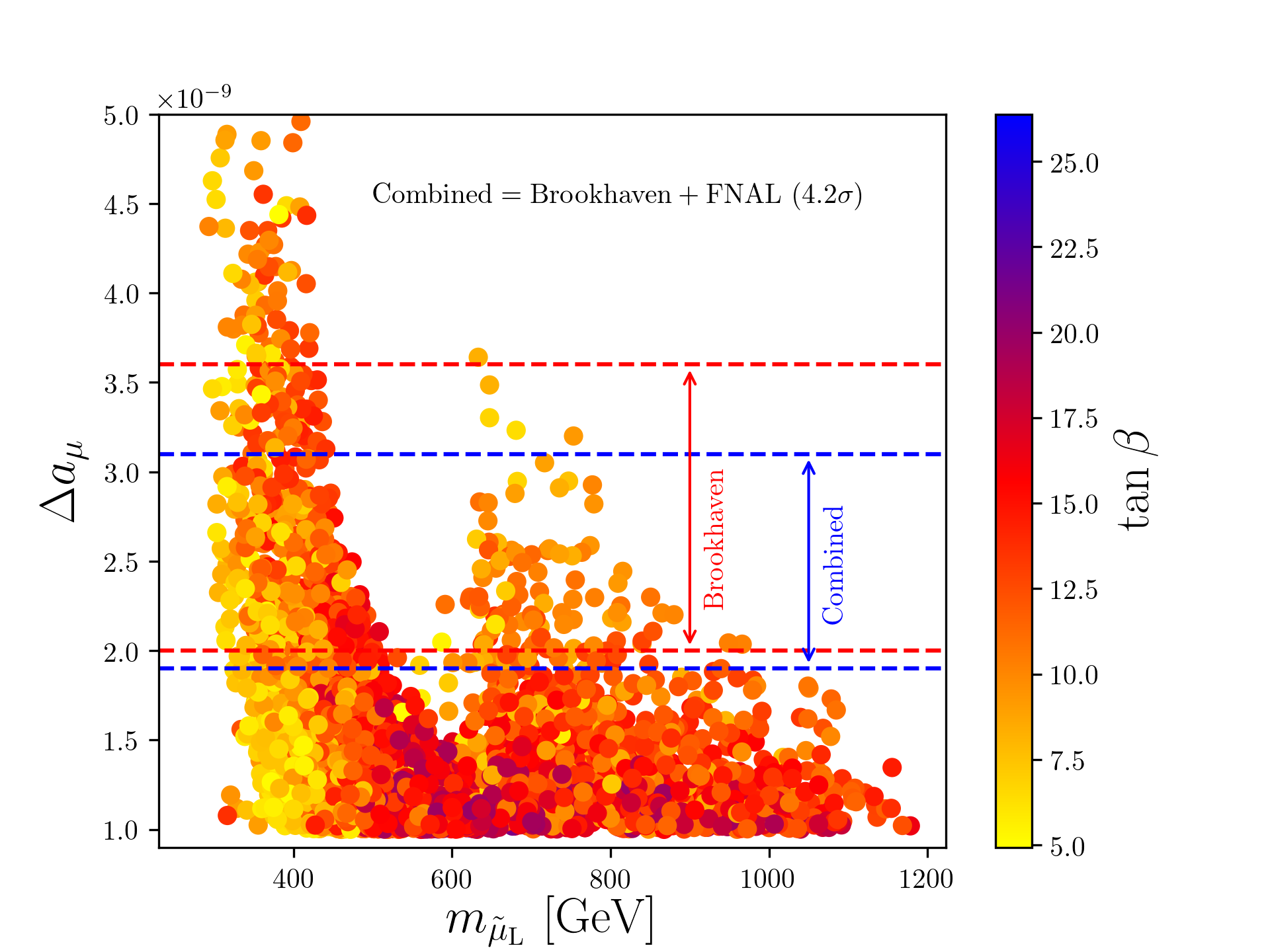
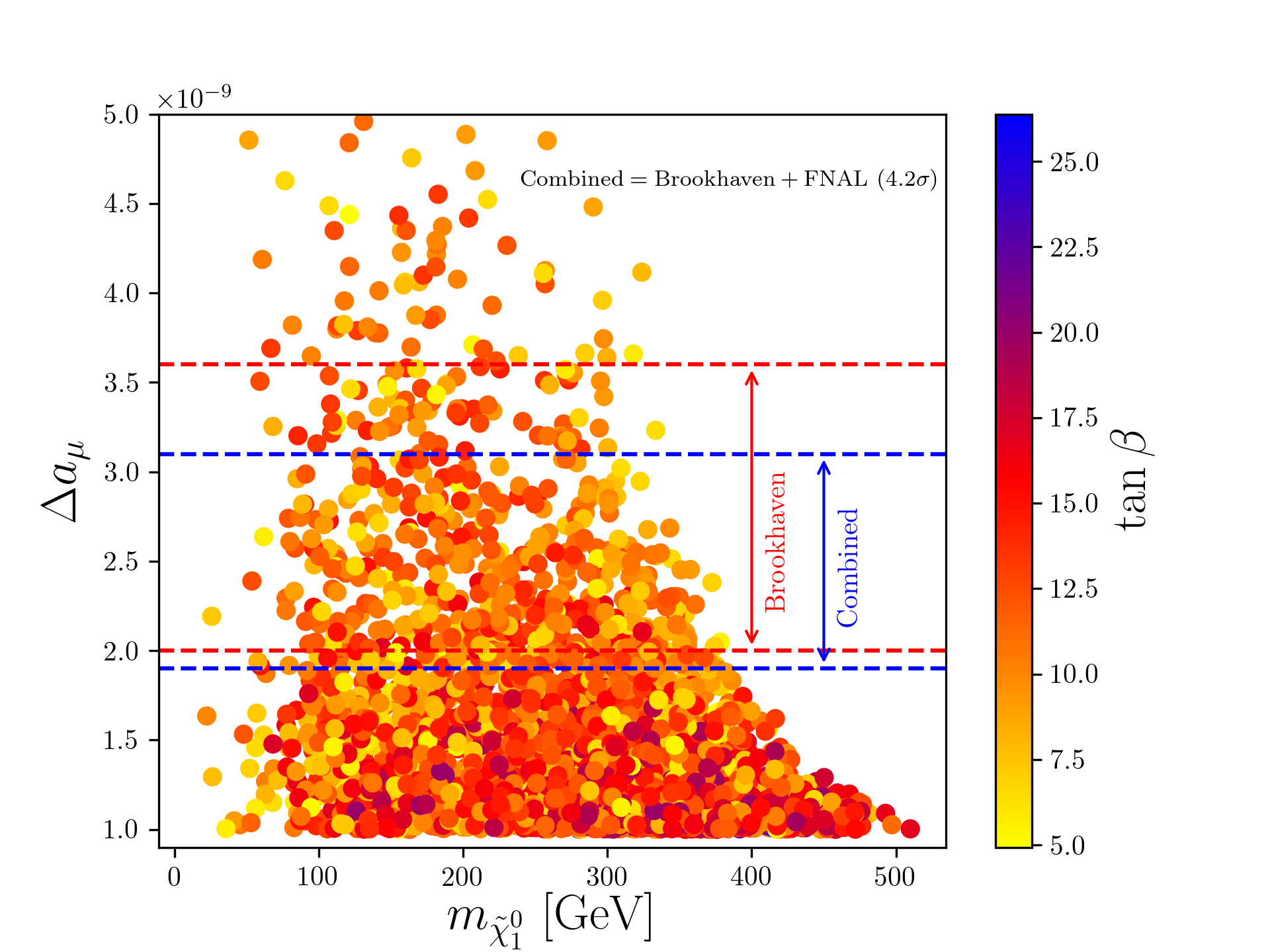
Figure 1: $\Delta a^{\rm SUSY}_{\mu}$ arising from the SUGRA parameter space using an ANN. The points satisfy the Higgs boson mass, the dark matter relic density and limits from dark matter direct detection experiments and the LHC. One sigma error corridor on $\Delta a_{\mu}$ experimental result from Brookhaven (red dashed lines) and from the combined Fermilab and Brookhaven result (blue dashed lines) are also displayed.

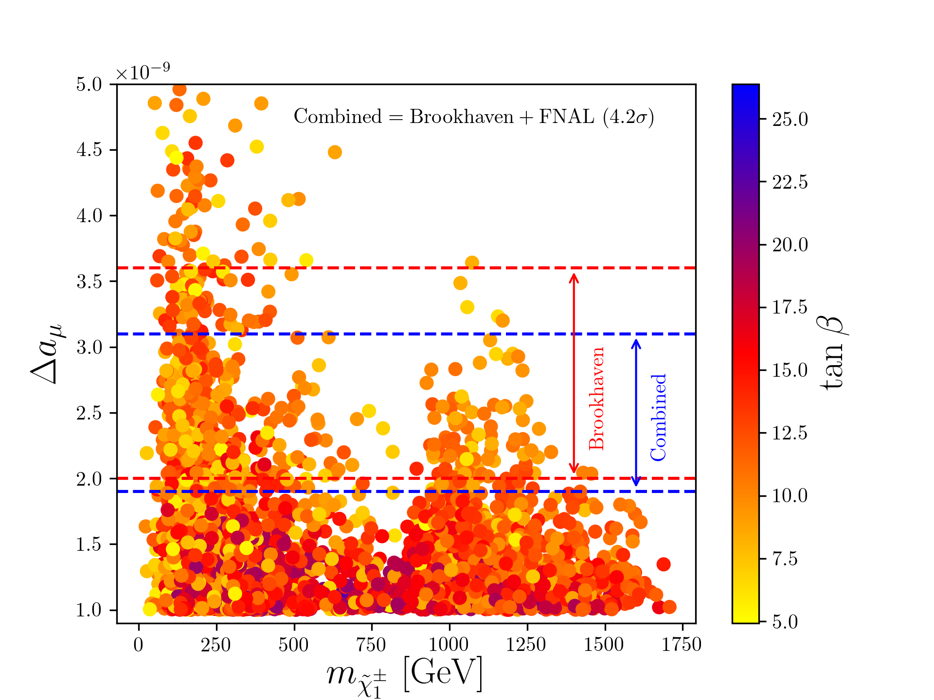
Figure 2: A scatter plot of $\Delta a_{\mu}$ versus the chargino mass as a result of a scan of the SUGRA parameter space using an artificial neural network. The points satisfy the Higgs boson mass, the dark matter relic density and limits from dark matter direct detection experiments and the LHC.

In Fig. 1 we display $\Delta a_{\mu}$ arising from supersymmetric loops vs the smuon mass (top panel) and vs the neutralino mass (bottom panel), while in Fig. 2 we show $\Delta a_{\mu}$ vs the chargino mass. The $\Delta a_{\mu}$ constraint with a one sigma corridor arising from the Brookhaven experiment and from the combined Fermilab and Brookhaven data are indicated and it is seen that the SUGRA model points populate the region allowed by the combined data constraint. In the analysis here we have not taken into account SUSY CP phases but we note in passing that SUSY CP phases can have significant effect on the supersymmetric loops corrections Aboubrahim:2016xuz . The constraints on SUSY phases arising from $\Delta{a^{\rm FB}_{\mu}}$ are discussed later.

Table 1: Input parameters for the benchmarks used in this analysis. All masses are in GeV.

Model	$m_{0}$	$A_{0}$	$m_{1}$	$m_{2}$	$m_{3}$	$\tan\beta$
​​(a)	460	-1209	726	378	5590	7.0
(b)	685	1380	868	493	8716	13.0
(c)	682	3033	875	714	8929	13.0
(d)	389	122	649	377	4553	8.2
(e)	254	1039	793	1477	8508	10.8

Table 2: The light sparticle spectrum consisting of the left and right handed sleptons ($\tilde{\ell}_{\rm L,R}$), the sneutrino ($\tilde{\nu}_{\rm L}$), neutralino ($\tilde{\chi}_{1}^{0}$), chargino ($\tilde{\chi}_{1}^{\pm}$) contributing to the muon $g-2$, the DM relic density and $\Delta a_{\mu}(\times 10^{-9})$ (calculated at the two-loop level using GM2Calc Athron:2015rva ). Also given are the SM-like Higgs mass, the spin-independent $(\times 10^{-51})$ and spin-dependent $(\times 10^{-49})$ proton-neutralino cross-section in units of cm².

Model	$h^{0}$	$\tilde{\ell}_{\rm L}$	$\tilde{\ell}_{\rm R}$	$\tilde{\nu}_{\rm L}$	$\tilde{\chi}^{0}_{1}$	$\tilde{\chi}^{\pm}_{1}$	$\Delta a_{\mu}$	$\Omega h^{2}$	$\sigma^{\rm SI}$	$\sigma^{\rm SD}$
​​(a)	123.7	313	542	304	222.2	222.4	2.13	0.001	5.17	9.13
(b)	124.6	412	761	405	271.7	271.9	3.04	0.002	1.62	5.27
(c)	124.6	501	758	495	331.0	465.0	2.02	0.055	4.73	9.63
(d)	123.4	305	463	295	237.4	237.6	2.33	0.002	13.0	49.2
(e)	123.7	721	422	716	300	1143	2.56	0.052	6.34	9.42

Table 3: The branching ratios for the dominant decay channels of the left and right handed sleptons along with the sneutrino.

Model	$\tilde{\ell}_{\rm L}\to\ell\tilde{\chi}^{0}_{1}$	$\tilde{\ell}_{\rm R}\to\ell\tilde{\chi}^{0}_{1}~{}[\tilde{\chi}^{0}_{2}]$	$\tilde{\nu}_{\rm L}\to\tilde{\chi}^{+}_{1}\ell^{-}$	$\tilde{\nu}_{\rm L}\to\tilde{\chi}^{0}_{1}\nu_{\ell}$
​​(a)	33%	- [100%]	66%	33%
(b)	32%	- [100%]	64%	32%
(c)	65%	100% [-]	20%	71%
(d)	31%	- [100%]	62%	30%
(e)	100%	100% [-]	-	100%

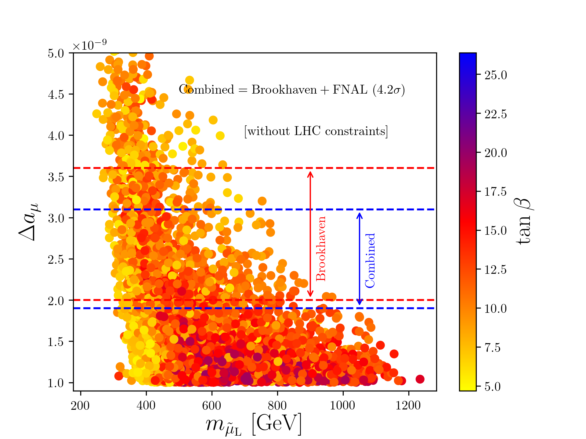
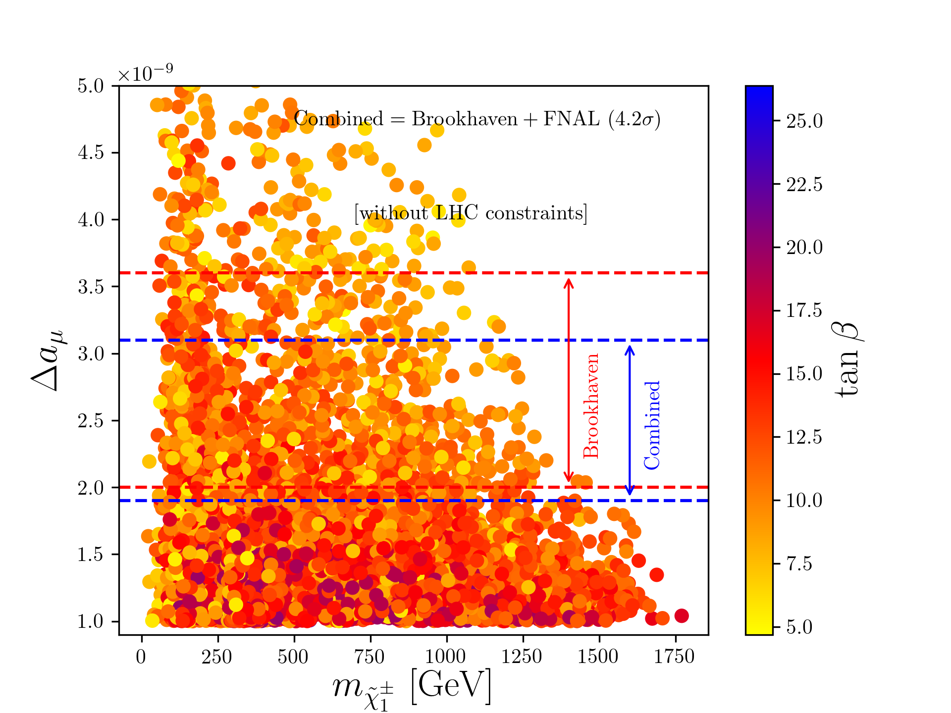
Figure 3: The same scatter plots as in Figs. 1 (top panel) and 2 but with the LHC constraints relaxed. We note that the dips in the model points in the smuon mass range near 600 GeV and in the chargino mass range near 800 GeV that appeared in Figs. 1 (top panel) and 2 are now populated.

One final remark about Figs. 1 and 2 is in order. The apparent dips in the density of models for smuons in the mass range near 600 GeV in Figs. 1 and for charginos in the mass range near 800 GeV in Figs. 2 are due to an imposition of the LHC constraints which exclude a significant number of models in this region. To exhibit this we give the same plots in Fig. 3 with the LHC constraints relaxed where one finds that the dips have disappeared.

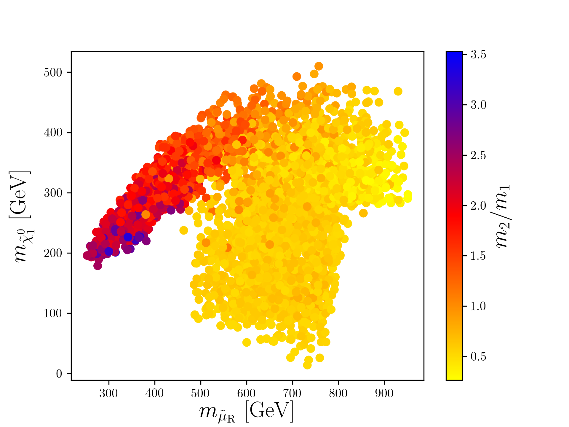
Figure 4: A scatter plot in the lightest neutralino mass-right handed smuon mass plane. The color axis denotes the ratio $m_{2}/m_{1}$. Notice that the larger $m_{2}/m_{1}$ is the lighter $\tilde{\mu}_{\rm R}$ becomes.

III 3. Sparticle spectrum and dark matter constrained by $\Delta{a^{\rm FB}_{\mu}}$

As noted already, the slepton, sneutrino and weakino mass spectrum arising from the $\Delta{a^{\rm FB}_{\mu}}$ constraint lie in the region of the parameter space with light and heavy particles, where the light particles with masses in the few hundred GeV range consisting of the neutralino, the chargino, the smuon and muon-sneutrino produce a significant correction to $\Delta a^{\rm SUSY}_{\mu}$ while the sparticles with color, and the remaining spectrum are significantly heavy lying in the several TeV region and do not participate in the loop corrections. The mass range of the light particles is shown in Fig. 5 where the top panel exhibits an illustrative mass range for the case when the chargino is the NLSP while the bottom panel is the case when the stau is the NLSP. The analysis shows that an smuon mass up to $\sim 1$ TeV, a chargino up to $\sim 1.5$ TeV and a neutralino up to $\sim 400$ GeV are allowed while being consistent with all constraints including $\Delta{a^{\rm FB}_{\mu}}$ and the current LHC limits. The smuon mass exhibited in Fig. 1 is that of the left handed smuon. While the right handed slepton is in general heavier than the left handed one, there are regions of the parameter space where the opposite is true. The spectrum shown in Table 2 illustrates this phenomena, where for benchmarks (a)$-$(d), $m_{\tilde{\ell}_{\rm L}}<m_{\tilde{\ell}_{\rm R}}$, except for benchmark (e) where $m_{\tilde{\ell}_{\rm L}}>m_{\tilde{\ell}_{\rm R}}$. The reason behind this is that $m_{2}>m_{1}$ here (see Table 1). To exhibit this more clearly we consider the left and right smuon masses at one loop so that

$$m^{2}_{\tilde{\mu}_{\rm L}} =m_{0}^{2}+m_{\mu}^{2}+C_{1}m_{1}^{2}+C_{2}m^{2}_{2}$$

$$+\left(-\frac{1}{2}+\sin^{2}\theta_{W}\right)M_{Z}^{2}\cos(2\beta)$$

$$m^{2}_{\tilde{\mu}_{\rm R}}= m_{0}^{2}+m_{\mu}^{2}+4C_{1}m_{1}^{2}-\sin^{2}\theta_{W}M_{Z}^{2}\cos(2\beta).$$

Here $C_{1}=\frac{3}{10}\tilde{\alpha}_{G}f_{1},C_{2}=\frac{3}{2}\tilde{\alpha}_{G}f_{2}$, where $\tilde{\alpha}_{G}=\alpha_{G}/(4\pi)$, $f_{k}(t)=t(2+b_{k}\tilde{\alpha}_{G}t)/(1+b_{k}\tilde{\alpha}_{G}t)^{2}$, $t=\ln(M_{G}^{2}/Q^{2})$ and $(b_{1},b_{2})=(33/5,1)$. Thus

$$m^{2}_{\tilde{\mu}_{\rm R}}-m^{2}_{\tilde{\mu}_{\rm L}} =3m_{1}^{2}C_{1}-m_{2}^{2}C_{2}$$

$$+\left(\frac{1}{2}-2\sin^{2}\theta_{W}\right)M_{Z}^{2}\cos(2\beta).$$

The $D$-term involving $M_{Z}$ is relatively small for the mass ranges we are considering, and a numerical estimate using $\alpha_{1}\sim 0.016,\alpha_{2}=0.033,\alpha_{G}\sim 0.04$ and $M_{G}\sim 1.2\times 10^{16}$ GeV gives $C_{1}\approx 0.16$ and $C_{2}\approx 0.23$. Thus one finds that typically the right smuon has a larger mass than the left smuon as is seen in benchmarks (a)$-$(d) unless $m_{2}\gtrsim 1.24m_{1}$ (with the assumed input) as seen in benchmark (e) and is supported by the analysis of Fig. 4.

$\Delta{a^{\rm FB}_{\mu}}$ also puts significant constraints on the spin-independent neutralino-nucleon cross section $\sigma_{\rm SI}$. As shown in Fig. 6, one finds that some of the models have $\sigma_{\rm SI}$ within reach of DARWIN Macolino:2020uqq and are thus discoverable. However, most of the allowed parameter space consistent with the $\Delta{a^{\rm FB}_{\mu}}$ constraint lies below the neutrino floor. The smallness of the $\sigma_{\rm SI}$ is a direct consequence of the fact that the neutralino is mostly a bino with only a small wino content.

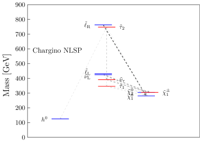
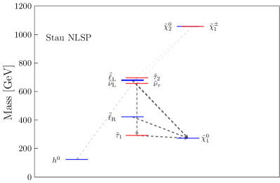
Figure 5: Exhibition of the light sparticle spectrum in $\tilde{g}$SUGRA models constrained by $\Delta{a^{\rm FB}_{\mu}}$. The top panel is for the case of chargino NLSP and bottom panel is for the stau NLSP. The plots are drawn using PySLHA Buckley:2013jua .

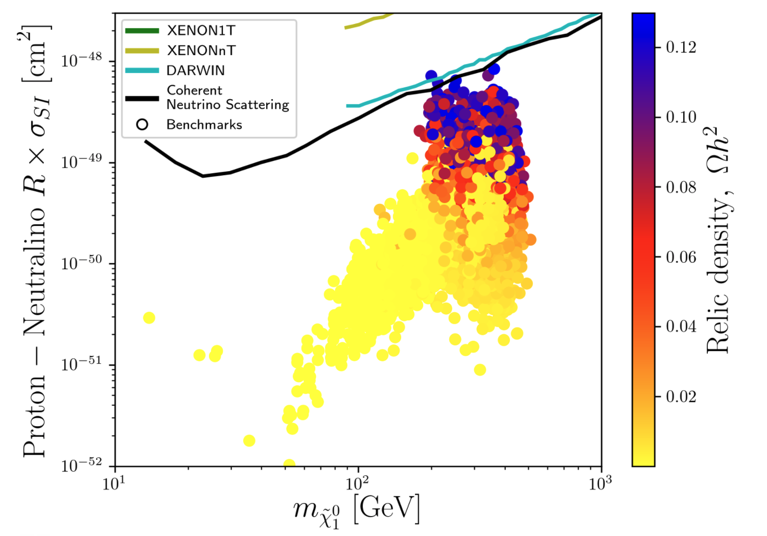
Figure 6: Spin-independent proton-neutralino cross section $\sigma_{\rm SI}$ as a function of the neutrino mass constrained by $\Delta{a^{\rm FB}_{\mu}}$. Here $R=\Omega h^{2}/(\Omega h^{2})_{\rm Planck}$ where $(\Omega h^{2})_{\rm Planck}\sim 0.12$.

IV 4. Implications of $\Delta{a^{\rm FB}_{\mu}}$ for discovering SUSY at HL-LHC and HE-LHC

The light sleptons and sneutrinos appearing in Table 2 could be pair produced in proton-proton collisions at 14 TeV (HL-LHC) and 27 TeV (HE-LHC). Another important production mode is the associated production of a slepton with an sneutrino which can have a significantly larger cross section than those of light sleptons and of light sneutrinos. The production cross-sections are computed at aNNLO+NNLL accuracy using Resummino-3.0 Debove:2011xj ; Fuks:2013vua and the five-flavor NNPDF23NLO PDF set and given in Tables 4 and 6. Slepton (selectron and smuon) and sneutrino production constitute a difficult signal region to look for at the LHC owing to their small production cross section and the decay topology resembling the SM backgrounds. The muon $g-2$ prefers smuons (and sneutrinos) with mass less than 1 TeV as one can see from Fig. 1 and their direct detection at the LHC is of importance especially after the recent $(g-2)_{\mu}$ results from Fermilab. Our signal consists of smuon (muon sneutrino) and selectron (electron sneutrino) pair production as well as slepton associated production with a sneutrino which decay to light leptons (electrons and muons) and a neutralino. The final states which make up our signal region involve two same flavor and opposite sign (SFOS) leptons with missing transverse energy (MET). We consider two main signal regions where for one signal region we require exactly one isolated jet which can be used to trigger on especially in an initial state radiation (ISR)-assisted topology when the MET is small, and for another signal region we require at least two jets targeting benchmarks with jetty final states. We call the former signal region SR-2$\ell$1j and the latter SR-2$\ell$2j. For such final states, the dominant SM backgrounds are from diboson production, $Z/\gamma+$jets, dilepton production from off-shell vector bosons ($V^{*}\rightarrow\ell\ell$), $t\bar{t}$ and $t+W/Z$. The subdominant backgrounds are Higgs production via gluon fusion ($ggF$ H) and vector boson fusion (VBF). The simulation of the signal and background events is performed at LO with MadGraph5_aMC@NLO-3.1.0 Alwall:2014hca interfaced to LHAPDF Buckley:2014ana using the NNPDF30LO PDF set. Up to two hard jets are added at generator level. The parton level events are passed to PYTHIA8 Sjostrand:2014zea for showering and hadronization using a five-flavor matching scheme in order to avoid double counting of jets. For the signal events, the matching/merging scale is set at one-fourth the mass of the pair produced sleptons or sneutrinos. Additional jets from ISR and FSR are added to the signal and background events. Jets are clustered with FastJet Cacciari:2011ma using the anti-$k_{t}$ algorithm Cacciari:2008gp with jet radius $R=0.4$. DELPHES-3.4.2 deFavereau:2013fsa is then employed for detector simulation and event reconstruction using the HL-LHC and HE-LHC card. The SM backgrounds are scaled to their relevant NLO cross sections while aNNLO+NNLL cross sections are used for the signal events.

Table 4: The aNNLO+NNLL pair production cross-sections, in fb, of sleptons at $\sqrt{s}=14$ TeV and at $\sqrt{s}=27$ TeV for benchmarks (a)$-$(e) of Table 1.

Model	$\sigma(pp\rightarrow\tilde{e}_{L}\,\tilde{e}_{L}~{}[\tilde{e}_{R}\,\tilde{e}_{R}])$		$\sigma(pp\rightarrow\tilde{\mu}_{L}\,\tilde{\mu}_{L}~{}[\tilde{\mu}_{R}\,\tilde{\mu}_{R}])$
	14 TeV	27 TeV	14 TeV	27 TeV
​​(a)	4.41 [0.159]	14.0 [0.684]	4.42 [0.159]	14.0 [0.684]
(b)	1.39 [0.028]	5.07 [0.168]	1.40 [0.028]	5.09 [0.168]
(c)	0.58 [0.029]	2.38 [0.171]	0.58 [0.029]	2.39 [0.171]
(d)	4.90 [0.328]	15.4 [1.27]	4.91 [0.328]	15.4 [1.27]
(e)	0.095 [0.493]	0.54 [1.79]	0.096 [0.495]	0.54 [1.80]

The discrimination between the signal and background events is done with the help of a deep neural network (DNN) as part of the ‘Toolkit for Multivariate Analysis’ (TMVA) Speckmayer:2010zz framework within ROOT6 Antcheva:2011zz . To train the signal and background events, we use a set of discriminating variables:

1. $E^{\rm miss}_{T}$: the missing transverse energy in the event. It is usually high for the signal due to the presence of neutralinos.

2. The transverse momentum of the leading non-b tagged jets, $p_{T}(j_{1})$. Rejecting b-tagged jets reduces the $t\bar{t}$ background.

3. The transverse momentum of the leading and subleading leptons (electron or muon), $p_{T}(\ell_{1})$ and $p_{T}(\ell_{2})$, respectively.

4. The total transverse momentum of all the ISR jets in an event, $p_{T}^{\rm ISR}$.

5. $M_{\rm T2}$, the stransverse mass Lester:1999tx ; Barr:2003rg ; Lester:2014yga of the leading and subleading leptons

   $$M_{\rm T2}=\min\left[\max\left(m_{\rm T}(\mathbf{p}_{\rm T}^{\ell_{1}},\mathbf{q}_{\rm T}),m_{\rm T}(\mathbf{p}_{\rm T}^{\ell_{2}},\,\mathbf{p}_{\rm T}^{\text{miss}}-\mathbf{q}_{\rm T})\right)\right],$$ (6)

   where $\mathbf{q}_{\rm T}$ is an arbitrary vector chosen to find the appropriate minimum and the transverse mass $m_{T}$ is given by

   $$m_{\rm T}(\mathbf{p}_{\rm T1},\mathbf{p}_{\rm T2})=\sqrt{2(p_{\rm T1}\,p_{\rm T2}-\mathbf{p}_{\rm T1}\cdot\mathbf{p}_{\rm T2})}.$$ (7)

6. The quantity $M^{\rm min}_{\rm T}$ defined as $M^{\rm min}_{\rm T}=\text{min}[m_{\rm T}(\textbf{p}_{\rm T}^{\ell_{1}},\textbf{p}^{\rm miss}_{\rm T}),m_{\rm T}(\textbf{p}_{\rm T}^{\ell_{2}},\textbf{p}^{\rm miss}_{\rm T})]$. The variables $M_{\rm T2}$ and $M^{\rm min}_{\rm T}$ are effective when dealing with large MET in the final state.

7. The dilepton invariant mass, $m_{\ell\ell}$, helps in rejecting the diboson background with a peak near the $Z$ boson mass which can be done by requiring $m_{\ell\ell}>100$ GeV.

8. The opening angle between the MET system and the dilepton system, $\Delta\phi(\textbf{p}_{\rm T}^{\ell},\textbf{p}^{\rm miss}_{\rm T})$, where $\textbf{p}_{\rm T}^{\ell}=\textbf{p}_{\rm T}^{\ell_{1}}+\textbf{p}_{\rm T}^{\ell_{2}}$.

9. The smallest opening angle between the first three leading jets in an event and the MET system, $\Delta\phi_{\rm min}(\textbf{p}_{\rm T}(j_{i}),\textbf{p}^{\rm miss}_{\rm T})$, where $i=1,2,3$.

It is worth mentioning how jets are classified as either coming from an ISR or from the decay of the SUSY system. After reconstructing the momentum of the dilepton system, we determine the angle between the dilepton system and each non-b-tagged jet in the event, i.e., $\Delta\phi(p_{T}(j_{i}),p_{T}^{\ell})$. If an event has exactly two jets with leading and subleading transverse momenta, $p_{T}(j_{1})$ and $p_{T}(j_{2})$, respectively, then both are tagged as non-ISR if $\Delta\phi(p_{T}(j_{1}),p_{T}^{\ell})<\Delta\phi(p_{T}(j_{2}),p_{T}^{\ell})$. However, if $\Delta\phi(p_{T}(j_{1}),p_{T}^{\ell})>\Delta\phi(p_{T}(j_{2}),p_{T}^{\ell})$, then the subleading jet is tagged as non-ISR and the leading one will be an ISR jet. If an event has more than two jets, then we select up to two jets that are closest to the dilepton system and tag them as non-ISR (possible jets arising from the decay of the SUSY system) and the rest are classified as ISR jets. Fig. 7 shows a 2D plot in the number of jets tagged as ISR ($y$ axis) versus the number of non-ISR jets ($x$ axis). One can see that the largest number of events correspond to the case of one ISR and one non-ISR jet per event. Moreover, one can get as many as six ISR jets in an event but with a low event count while a larger number of events have no ISR jets.

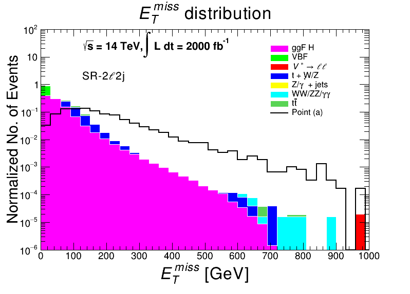
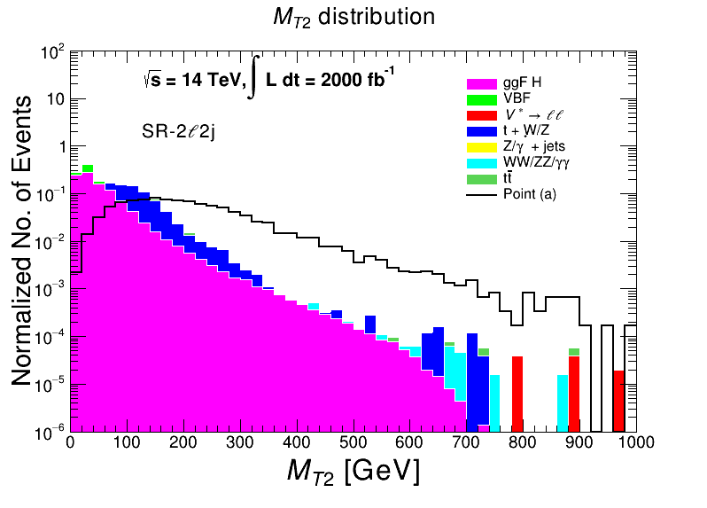
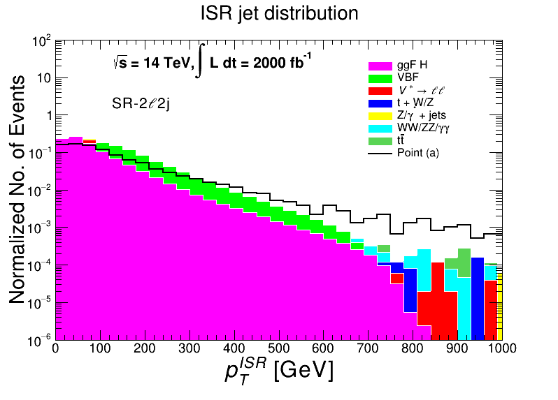
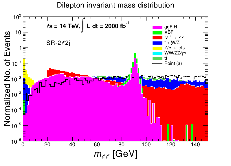
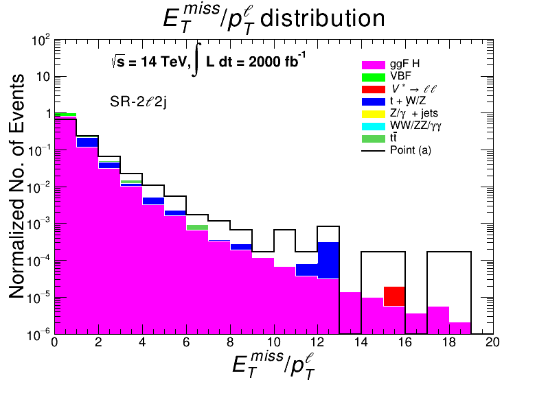
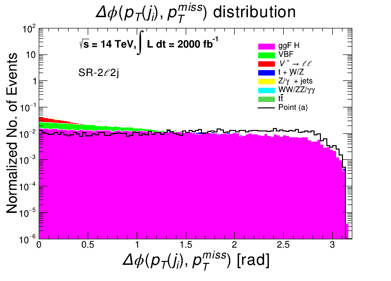
Figure 8: A sample of the discriminating variables using by the DNN for training and testing. The distributions are in the normalized number of events scaled by a specific integrated luminosity to show the discriminating power of each variable.

Fig. 8 shows normalized distributions in six of the discriminating variables which are used by the DNN for training. Before the events are fed into a DNN, a set of preselection criteria is applied to the signal and background. The leading and subleading leptons must have a transverse momenta $p_{T}>15$ GeV for electrons and $p_{T}>10$ GeV for muons with $|\eta|<2.5$. Each event in SR-2$\ell$1j should contain exactly one non-b-tagged jet while in SR-2$\ell$2j at least two non-b-tagged jets are required with the leading $p_{T}>20$ GeV in the $|\eta|<2.4$ region and $E^{\rm miss}_{T}>100$ GeV. The preselection criteria are summarized in Table 5.

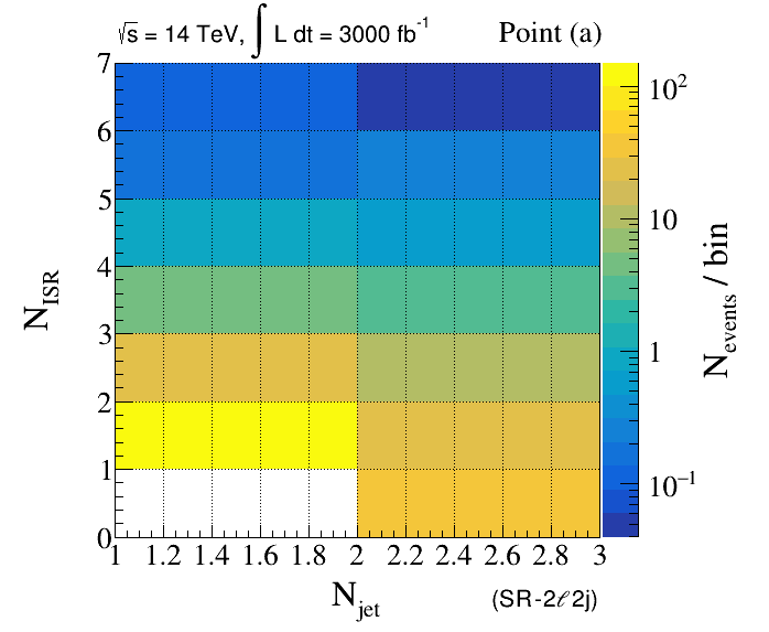
Figure 7: A two-dimensional plot in the number of ISR jets ($N_{\rm ISR}$) versus non-ISR jets ($N_{\rm jet}$).

IV.1 Slepton pair production

We begin the analysis with the first production mode which is slepton pair production. Table 4 shows the pair production cross sections of left handed and right handed sleptons for the benchmarks of Table 1 at 14 TeV and 27 TeV. Notice that the contribution from right handed sleptons is small compared to the left handed ones except for benchmark (e) where $m_{\tilde{\ell}_{\rm R}}<m_{\tilde{\ell}_{\rm L}}$. In this model point, the right handed slepton has a mass $\sim 400$ GeV which is comparable to the left handed slepton of benchmark (b). However, the cross section is smaller as one expects. Those benchmarks represent a contrast between high scale models and simplified models considered in LHC analyses. Thus, in ATLAS and CMS analyses, left and right handed sleptons are considered to be of the same mass and are excluded on an equal footing. In our case, however, we must consider the two particles separately. Of course, if a specific benchmark has a left (right) handed slepton which is excluded by experiment then this would eliminate the entire benchmark regardless of the mass of its right (left) handed counterpart. In this analysis we focus on the left handed sleptons knowing that the right handed ones have less significant contribution but we make sure that the right handed sleptons are not excluded as this would entirely eliminate the benchmark under study. An exception to this situation is benchmark (e), where despite having a small $\tilde{\ell}_{\rm R}\tilde{\ell}_{\rm R}$ production cross section compared to its left handed counterpart of the same mass, the branching ratio of $\tilde{\ell}_{\rm R}$ to $\ell\tilde{\chi}^{0}_{1}$ is unity (see Table 3) which makes $\sigma\times\text{BR}$ significant. Hence in this benchmark, we simulate both the left and right handed sleptons. Another aspect of high scale models which differentiates our analysis from that of LHC concerns the branching ratios of slepton and sneutrino decays. The relevant branching ratios are given in Table 3 and unlike LHC analyses which consider a unit branching fraction to leptons and neutralinos, our benchmarks have a more diverse decay topology. Next, we present the results from the two signal regions SR-2$\ell$2j and SR-2$\ell$1j defined earlier.

The signal region SR-2$\ell$2j:

To train and test the signal ($S$) and background ($B$) events that have passed the preselection criteria, a four-layer DNN uses two statistically independent sets of signal and background events. The training phase employs the above set of variables to create a new powerful kinematic variable called the ‘DNN response’ which can be used as a discriminant to reject events thus maximizing the $S/\sqrt{S+B}$ ratio. Fig. 9 shows distributions in the DNN response for benchmark (a) at 14 TeV and 27 TeV. The DNN has successfully separated the signal events which can be seen peaking near 1 while the SM background is more concentrated at values less than 1. The cut on the DNN response is aided by a series of analysis cuts using some of the variables described above. A summary of the preselection criteria and the analysis cuts is given in Table 5. A minimum cut on $\mathrm{DNN~{}response}>0.95$ removes most of the background and benchmarks (a)$-$(e) become discoverable at both HL-LHC and HE-LHC. The estimated integrated luminosities for discovery are shown in the last two columns of Table 5. It is worth mentioning that benchmark (e) becomes discoverable at HL-LHC only when the contribution from right handed sleptons is included. We note that the cuts need to be customized when studying HE-LHC as compared to HL-LHC.

Table 5: The analysis uses cuts on a set of kinematic variables at 14 TeV (27 TeV) grouped by the benchmarks of Table 1 in two signal regions SR-$2\ell 1$j and SR-$2\ell 2$j. We note that with the exception of $m_{\ell\ell}$ harder cuts are applied at 27 TeV. Entries with a dash (-) imply that no requirement on the variable is considered. Shown at the bottom of the table are the integrated luminosities needed for discovery at 14 TeV and 27 TeV. Also shown are the preselection criteria used.

Observable	(a), (b), (d)	(c)	(e)	(a), (b), (d)	(c)	(e)
	Preselection criteria (SR-$2\ell 2$j)			Preselection criteria (SR-$2\ell 1$j)
$N_{\ell}$ (SFOS)	$2$			$2$
$N_{\rm jets}^{\rm non-b-tagged}$	$\geq 2$			$1$
$p_{T}(j_{1})$ [GeV]	$>20$			$>20$
$p_{T}(\ell_{1})$ (electron, muon) [GeV]	$>15$, $>10$			$>15$, $>10$
$E^{\rm miss}_{T}$ [GeV]	$>100$			$>100$
	Analysis cuts			Analysis cuts
​​ $m_{\ell\ell}~{}\text{[GeV]}>$	130	150	150 (110)	130 (240)	200 (150)	150 (110)
$E^{\rm miss}_{T}/\textbf{p}^{\ell}_{\rm T}>$	0.5 (2.8)	-	-	1.0 (1.5)	-	-
$\Delta\phi_{\rm min}(\textbf{p}_{\rm T}(j_{i}),\textbf{p}^{\rm miss}_{\rm T})~{}\text{[rad]}>$	-	0.85 (1.5)	-	-	0.80 (1.5)	-
$p_{T}(\ell_{2})~{}\text{[GeV]}>$	-	-	190 (370)	-	-	190 (300)
$M_{T2}~{}\text{[GeV]}>$	120 (140)	120	200 (300)	-	120	200 (300)
DNN response $>$	0.95	0.95	0.95	0.95	0.95	0.95
$\mathcal{L}$ at 14 TeV [fb-1]	1629, 1559, 1371	664	1292	426, 853, 478	2742	923
$\mathcal{L}$ at 27 TeV [fb-1]	716, 1432, 535	314	827	306, 387, 347	830	572

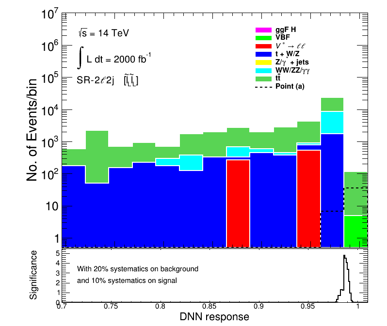
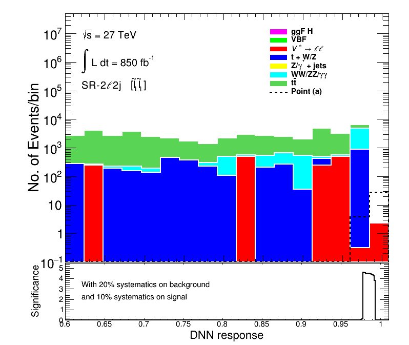
Figure 9: Distributions in the DNN response for the signal (dashed histogram) and background (colored histograms) events pertaining to benchmark (a) at 14 TeV (top panel) and 27 TeV (bottom panel) for the signal region SR-$2\ell 2$j in the slepton pair production channel. The bottom pad of each panel shows the significance as defined by Eq. (8) as a function of the cut on the ‘DNN response’ variable. The binning for the significance distribution is finer to clearly show the rise and fall of the significance.

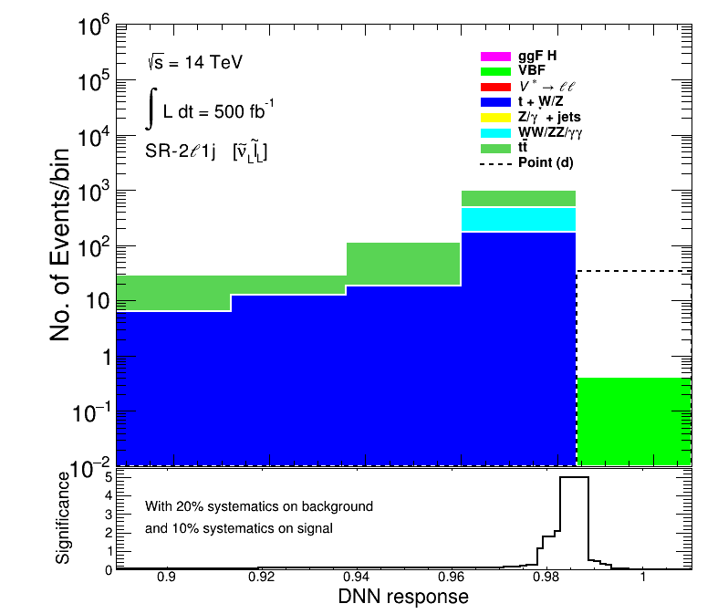
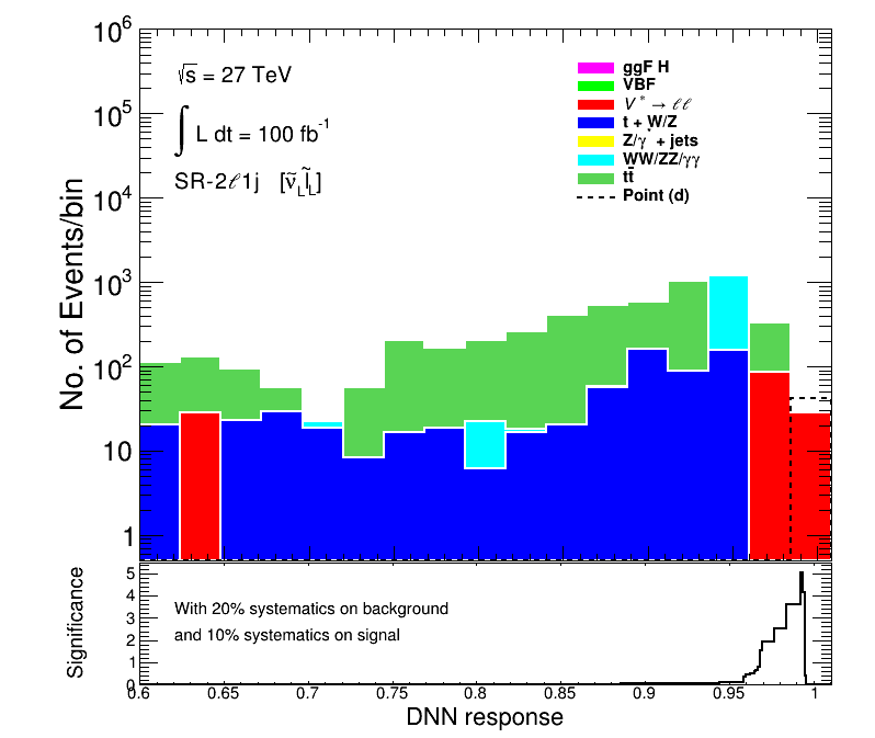
Figure 10: Distributions in the DNN response for the signal (dashed histogram) and background (colored histograms) events pertaining to benchmark (d) at 14 TeV (top panel) and 27 TeV (bottom panel) for the signal region SR-$2\ell 1$j in the slepton associated production channel. The bottom pad of each panel shows the significance as defined by Eq. (8) as a function of the cut on the ‘DNN response’ variable. The binning for the significance distribution is finer to clearly show the rise and fall of the significance.

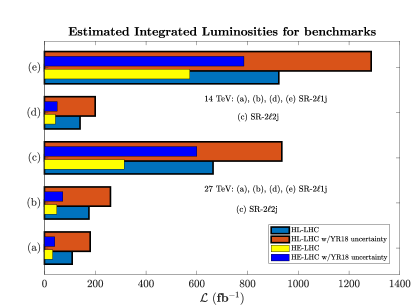
Figure 11: The integrated luminosities needed for discovery of SUSY at HL-LHC and HE-LHC assuming that $\Delta{a^{\rm FB}_{\mu}}$ arises from SUSY loops. The signal regions and production modes shown are the ones giving the highest sensitivity for discovery. Also shown are the integrated luminosities after including the ‘YR18’ uncertainties on the signal and background.

The signal region SR-2$\ell$1j:

In this signal region, we require only one non-b-tagged jet which has the potential of offering a greater sensitivity Aad:2019vnb . In this signal region, we do not differentiate between ISR and non-ISR jets. Therefore the variable $p_{T}^{\rm ISR}$ is not used here. Using the same DNN training and testing technique discussed in the preceding analysis, we construct the ‘DNN response’ variable and apply the selection criteria specific to this signal region as shown in Table 5. We then estimate the integrated luminosity required for a $5\sigma$ discovery for each benchmark. The results are shown in the last two columns of Table 5. We note that that the single jet signal region provides a greater sensitivity for detection relative to the two jet signal for benchmarks (a), (b) and (d). On the other hand the two-jet signal region shows a better detection sensitivity for benchmark (c) than the single jet signal region. The reason is that benchmark (c) has a stau which is the NLSP. So the decay channels $\tilde{\ell}_{\rm L}\to\tilde{\chi}^{0}_{2}\ell\to\tilde{\tau}\tau\ell\to\tau\tau\ell\tilde{\chi}^{0}_{1}$ and $\tilde{\ell}_{\rm L}\to\tilde{\chi}_{1}^{-}\nu_{\ell}\to\tau\nu_{\tau}\nu_{\ell}\tilde{\chi}^{0}_{1}$ render a tau-enriched final state. Since taus can form jets, then requiring at least two jets in SR-2$\ell$2j does lead to a better sensitivity than SR-2$\ell$1j.

IV.2 Sneutrino pair production

According to Table 3, the decay channel $\tilde{\nu}_{\rm L}\to\tilde{\chi}^{+}_{1}\ell^{-}$ has a significant branching ratio for benchmarks (a), (b) and (d) which correspond to the case of a chargino NLSP. Since the chargino and the LSP are nearly degenerate, the decay products cannot be discerned and therefore would contribute to the total MET. In this case, the final states will be identical to the slepton pair production mode discussed in the previous section. The sneutrino pair production cross section at aNNLO+NNLL is given in Table 6 for benchmarks (a), (b) and (d). Since we have already shown that the signal region SR-$2\ell 1$j provides a better sensitivity for these benchmarks, we will use it again to estimated the required integrated luminosity for discovery at 14 TeV and 27 TeV. The results are shown in Table 7. In comparison to slepton pair production, the sneutrino pair production mode fairs better at the chances of discovering SUSY with benchmark (d) requiring only 317 fb^-1 of integrated luminosity which should become available in the next round of data taking at the LHC. That is contrasted with 1371 fb^-1 needed in SR-$2\ell 2$j and 478 fb^-1 in SR-$2\ell 1$j for the slepton pair production mode as shown in Table 5.

Table 6: The aNNLO+NNLL pair production cross-sections, in fb, of sneutrinos and the slepton associated production at $\sqrt{s}=14$ TeV and at $\sqrt{s}=27$ TeV for benchmarks (a), (b) and (d) of Table 1.

Model	$\sigma(pp\rightarrow\tilde{\nu}_{L}\,\tilde{\nu}_{L})$		$\sigma(pp\rightarrow\tilde{\nu}_{L}\,\tilde{\ell}_{L})$
	14 TeV	27 TeV	14 TeV	27 TeV
​​(a)	9.37	29.82	37.63	116.38
(b)	2.80	10.25	11.76	41.56
(d)	10.52	33.10	41.78	127.80

Table 7: The estimated integrated luminosities, in fb^-1, for discovery of benchmarks (a), (b) and (d) of Table 1 at 14 TeV and 27 TeV for the cases of sneutrino pair production and slepton associated production with a sneutrino.

Model	SR-$2\ell 1$j [$\tilde{\nu}_{L}\,\tilde{\nu}_{L}$]		SR-$2\ell 1$j [$\tilde{\nu}_{L}\,\tilde{\ell}_{L}$]
	$\mathcal{L}$ at 14 TeV	$\mathcal{L}$ at 27 TeV	$\mathcal{L}$ at 14 TeV	$\mathcal{L}$ at 27 TeV
​​(a)	367	87	257	39
(b)	685	127	295	68
(d)	317	65	232	32

IV.3 Slepton associated production with a sneutrino

Finally, we consider the associated production of a slepton with an sneutrino for the benchmarks (a), (b) and (d) and for the same reason discussed in the sneutrino pair production case. In addition, this production mode proceeds through the charged current and thus has a larger cross section as one can see from Table 6. This leads to a lower integrated luminosity for discovery at both HL-LHC and HE-LHC as illustrated in Table 7. Fig. 10 shows the distributions in the DNN response for benchmark (d) in the single jet signal region at 14 TeV and 27 TeV for the slepton associated production channel.

Next, we discuss the systematic uncertainties associated with the signal and the background and their effect on the predicted integrated luminosities.

V 5. Discovery significance for benchmarks

The integrated luminosity for a $5\sigma$ discovery is re-estimated after including the systematic uncertainties using the signal significance

$$\sigma=\frac{S}{\sqrt{S+B+(\delta_{S}S)^{2}+(\delta_{B}B)^{2}}},$$ (8)

where $\delta_{S}$ and $\delta_{B}$ are the systematic uncertainties in the signal and background estimates. The recommendations on systematic uncertainties (known as ‘YR18’ uncertainties) published in the CERN’s yellow reports CidVidal:2018eel ; Cepeda:2019klc suggest an overall 20% uncertainty in the background and 10% in the SUSY signal. The bottom pads of each of the panels in Figs. 9 and 10 show the distribution in the signal significance of Eq. (8) as a function of the cut on ‘DNN response’. We adopt a finer binning in the bottom pads as compared to the upper ones in order to properly show how the significance changes with the cut. We notice that a higher integrated luminosity is required after including the systematics but are still within the reach of HL-LHC and HE-LHC.

Next, we combine the different production channels discussed earlier to present the final integrated luminosities for discovery of the benchmarks of Table 1. We show in Fig. 11 the integrated luminosities for benchmarks (a)$-$(e) before and after including the ‘YR18’ uncertainties and combining the different production channels at HL-LHC and HE-LHC. The signal regions shown are the ones which give us the best sensitivity for SUSY discovery. We also show the integrated luminosities for discovery of the benchmarks in Table 8 after including systematic uncertainties in the signal and background. Thus, benchmarks (a), (b) and (d) are discoverable with $\mathcal{L}\sim 180$ to $\sim 260$ fb^-1 at 14 TeV while the estimate drops to $\sim 40$ to $\sim 72$ fb^-1 at 27 TeV. In both cases, the most optimal signal region is SR-$2\ell 1$j. For benchmark (c), $\mathcal{L}\sim 900$ fb^-1 is required at HL-LHC and $\sim 600$ fb^-1 at HE-LHC with SR-$2\ell 2$j being the optimal signal region. Lastly, benchmark (e) can be discovered at HL-LHC with $\sim 1300$ fb^-1 while $\sim 780$ fb^-1 of integrated luminosity is needed at HE-LHC with SR-$2\ell 1$j being the optimal signal region for discovery.

One final remark regarding the LHC phenomenology in this analysis. Benchmarks (c) and (e) exhibit light charginos and second neutralinos with a considerable mass gap between those particles on one hand and the neutralino LSP on another. Thus here one should also consider electroweakino pair production, $\tilde{\chi}^{0}_{2}\tilde{\chi}^{\pm}_{1}$ and $\tilde{\chi}^{+}_{1}\tilde{\chi}^{-}_{1}$. However, in neither of those benchmarks the charginos and the second neutralinos are the NLSP and it is the stau which is the NLSP. Further, in benchmark (e), $\tilde{\chi}^{0}_{2}$ and $\tilde{\chi}^{\pm}_{1}$ are heavier than the sleptons and the staus. For this reason, the branching ratio to SFOS leptons is greatly reduced especially for benchmark (c) where the electroweakinos decay to staus which eventually decay to a tau and an LSP. Of course, a tau can decay leptonically but this branching ratio is suppressed in comparison to its hadronic decays. Despite the larger production cross sections, the overall $\sigma\times\text{BR}$ turns out to be smaller than the other production modes considered in this paper. Thus the electroweakinos do not constitute a strong discovery channel for the benchmarks discussed here. The interested reader is directed to earlier works on SUSY discovery with electroweakino production Aboubrahim:2017wjl , including the clean three-lepton channel Aboubrahim:2018bil .

Table 8: The estimated integrated luminosities, in fb^-1, for discovery of benchmarks of Table 1 at 14 TeV and 27 TeV after combining all production channels and including systematics in the signal and background.

Model	SR-$2\ell 1$j		SR-$2\ell 2$j
	$\mathcal{L}$ at 14 TeV	$\mathcal{L}$ at 27 TeV	$\mathcal{L}$ at 14 TeV	$\mathcal{L}$ at 27 TeV
​​(a)	180	40	1863	950
(b)	260	72	1720	1550
(c)	3155	1060	935	600
(d)	200	50	1860	715
(e)	1287	786	1437	1175

VI 6. Constraints on CP phases from $\Delta{a^{\rm FB}_{\mu}}$

It is known that SUSY CP violating phases arising from the soft parameters can have significant effect on $a_{\mu}^{\rm SUSY}$ Ibrahim:1999aj ; Ibrahim:2001ym . Here we discuss the phase dependence of the chargino contribution which is the dominant one, although the analysis is done including both the chargino and the neutralino exchange contributions. For the chargino exchange contribution the phases enter via the chargino mass matrix

$$M_{C}=\begin{pmatrix}|m_{2}|e^{i\xi_{2}}&\sqrt{2}m_{W}\sin\beta\\ \sqrt{2}m_{W}\cos\beta&|\mu|e^{i\theta_{\mu}}\\ \end{pmatrix},$$ (9)

where $\theta_{\mu}$ is the phase of the Higgs mixing parameter $\mu$, and $\xi_{2}$ is the phase of the SU(2) gaugino mass $m_{2}$. The chargino contribution is given by Ibrahim:1999aj

$$a^{\chi^{+}}_{\mu} =\frac{m_{\mu}\alpha_{EM}}{4\pi\sin^{2}\theta_{W}}\sum_{i=1}^{2}\frac{1}{m_{\chi_{i}^{+}}}\text{Re}(\kappa_{\mu}U^{*}_{i2}V^{*}_{i1})F_{3}\left(\frac{m^{2}_{\tilde{\nu}}}{m^{2}_{\tilde{\chi}_{i}^{+}}}\right)$$ (10)

$$+\frac{m^{2}_{\mu}\alpha_{EM}}{24\pi\sin^{2}\theta_{W}}\sum_{i=1}^{2}\frac{1}{m^{2}_{\chi_{i}^{+}}}(|\kappa_{\mu}U^{*}_{i2}|^{2}+|V_{i1}|^{2})F_{4}\left(\frac{m^{2}_{\tilde{\nu}}}{m^{2}_{\tilde{\chi}_{i}^{+}}}\right),$$

where the form factors are given by

$$F_{3}(x) =\frac{1}{(x-1)^{3}}(3x^{2}-4x+1-2x^{2}\ln x),$$ (11)

$$F_{4}(x) =\frac{1}{(x-1)^{4}}(2x^{3}+3x^{2}-6x+1-6x^{2}\ln x)\,.$$

In Eq. (10), $U$ and $V$ are defined so that $U^{*}M_{C}V^{-1}=\text{diag}(m_{\tilde{\chi}^{+}_{1}},m_{\tilde{\chi}^{+}_{2}})$, where $U$ and $V$ are unitary matrices, and where $\kappa_{\mu}={m_{\mu}}/{\sqrt{2}m_{W}\cos\beta}$.

The neutralino contribution is given by

$$a^{\chi^{0}}_{\mu} =\frac{m_{\mu}\alpha_{\rm EM}}{4\pi\sin^{2}\theta_{W}}\sum_{j=1}^{4}\sum_{k=1}^{2}\frac{1}{m_{\tilde{\chi}^{0}_{j}}}\text{Re}(\eta^{k}_{\mu j})F_{1}\left(\frac{m^{2}_{\tilde{\mu}_{k}}}{m^{2}_{\tilde{\chi}^{0}_{j}}}\right)$$

$$+\frac{m^{2}_{\mu}\alpha_{\rm EM}}{24\pi\sin^{2}\theta_{W}}\sum_{j=1}^{4}\sum_{k=1}^{2}\frac{1}{m^{2}_{\tilde{\chi}^{0}_{j}}}X^{k}_{\mu j}F_{2}\left(\frac{m^{2}_{\tilde{\mu}_{k}}}{m^{2}_{\tilde{\chi}^{0}_{j}}}\right),$$ (12)

where

$$\eta^{k}_{\mu j} =-\frac{1}{\sqrt{2}}\Big{(}\tan\theta_{W}X_{1j}D^{*}_{1k}+X_{2j}D^{*}_{1k}-\sqrt{2}\kappa_{\mu}X_{3j}D^{*}_{2k}\Big{)}$$

$$\hskip 22.76228pt\times\Big{(}\sqrt{2}\tan\theta_{W}X_{1j}D_{2k}+\kappa_{\mu}X_{3j}D_{1k}\Big{)},$$ (13)

and

$$X^{k}_{\mu j} =|D_{1k}|^{2}\text{Re}(X_{1j}X^{*}_{2j})\tan\theta_{W}+\frac{m^{2}_{\mu}}{2m^{2}_{W}\cos^{2}\beta}|X_{3j}|^{2}$$

$$+\frac{1}{2}\tan^{2}\theta_{W}|X_{1j}|^{2}(|D_{1k}|^{2}+4|D_{2k}|^{2})$$

$$-\frac{m_{\mu}}{m_{W}\cos\beta}\text{Re}(X_{3j}X^{*}_{2j}D_{1k}D^{*}_{2k})+\frac{1}{2}|X_{2j}|^{2}|D_{1k}|^{2}$$

$$+\frac{m_{\mu}\tan\theta_{W}}{m_{W}\cos\beta}\text{Re}(X_{3j}X^{*}_{1j}D_{1k}D^{*}_{2k}).$$ (14)

In Eq. (14), $X$ is a unitary matrix that diagonalizes the symmetric neutralino mass matrix, so that $X^{T}M_{\tilde{\chi}^{0}}X=\text{diag}(m_{\tilde{\chi}^{0}_{1}},m_{\tilde{\chi}^{0}_{2}},m_{\tilde{\chi}^{0}_{3}},m_{\tilde{\chi}^{0}_{4}})$, and $D$ diagonalizes the hermitian smuon mass square matrix, $D^{\dagger}M^{2}_{\tilde{\mu}}D=\text{diag}(m^{2}_{\tilde{\mu}_{1}},m^{2}_{\tilde{\mu}_{2}})$. The form factors in Eq. (12) are given by

$$F_{1}(x) =\frac{1}{(x-1)^{3}}(1-x^{2}+2x\ln x),$$ (15)

$$F_{2}(x) =\frac{1}{(x-1)^{4}}(-x^{3}+6x^{2}-3x-2-6x\ln x)\,.$$

The phases enter via $U,V,X$ and through the chargino and neutralino masses. We note that the phase dependence of the chargino contribution to $a_{\mu}$ arises entirely from the combination $\theta_{\mu}+\xi_{2}$. The neutralino contribution, however, has additional phase dependence from $\xi_{1}$, the phase of $m_{1}$, and from $\alpha_{A_{0}}$, the phase of $A_{0}$. In Fig. 12 we show the sensitivity of $\Delta{a^{\rm FB}_{\mu}}$ to CP phases $\xi_{1}$ and $\xi_{2}$.

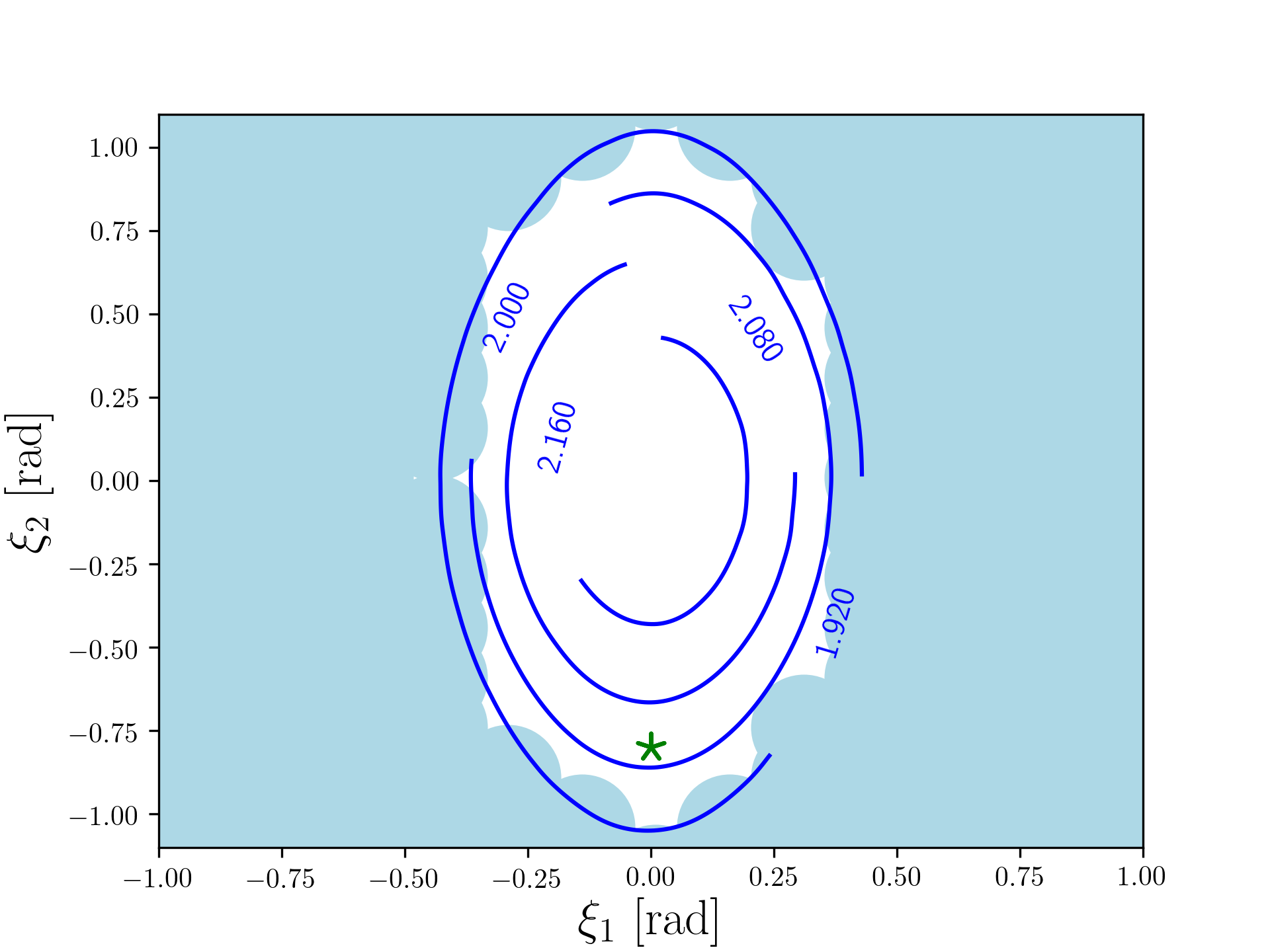
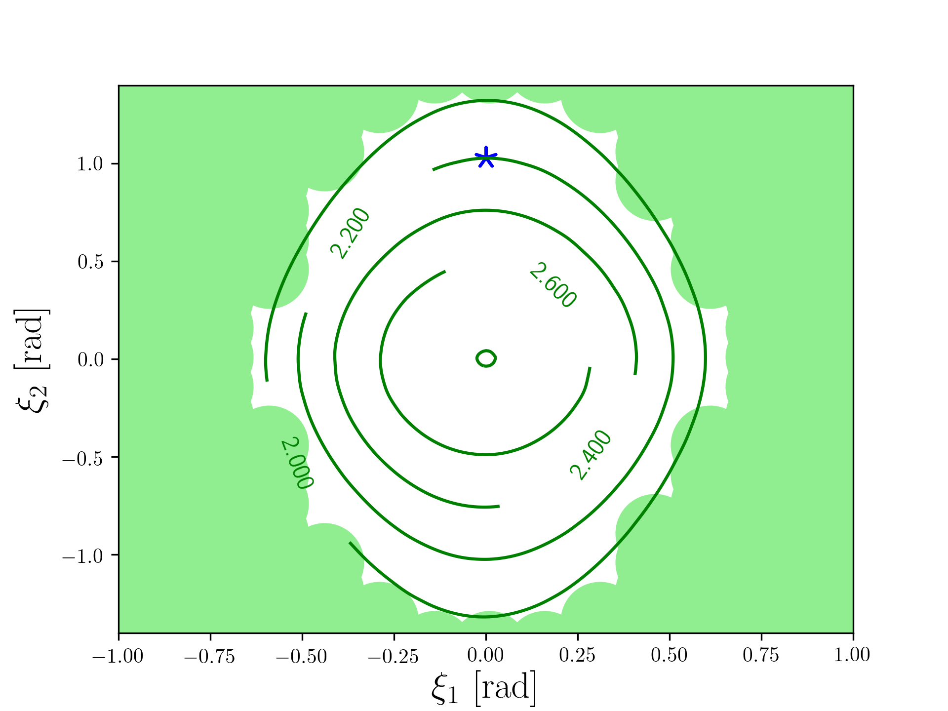
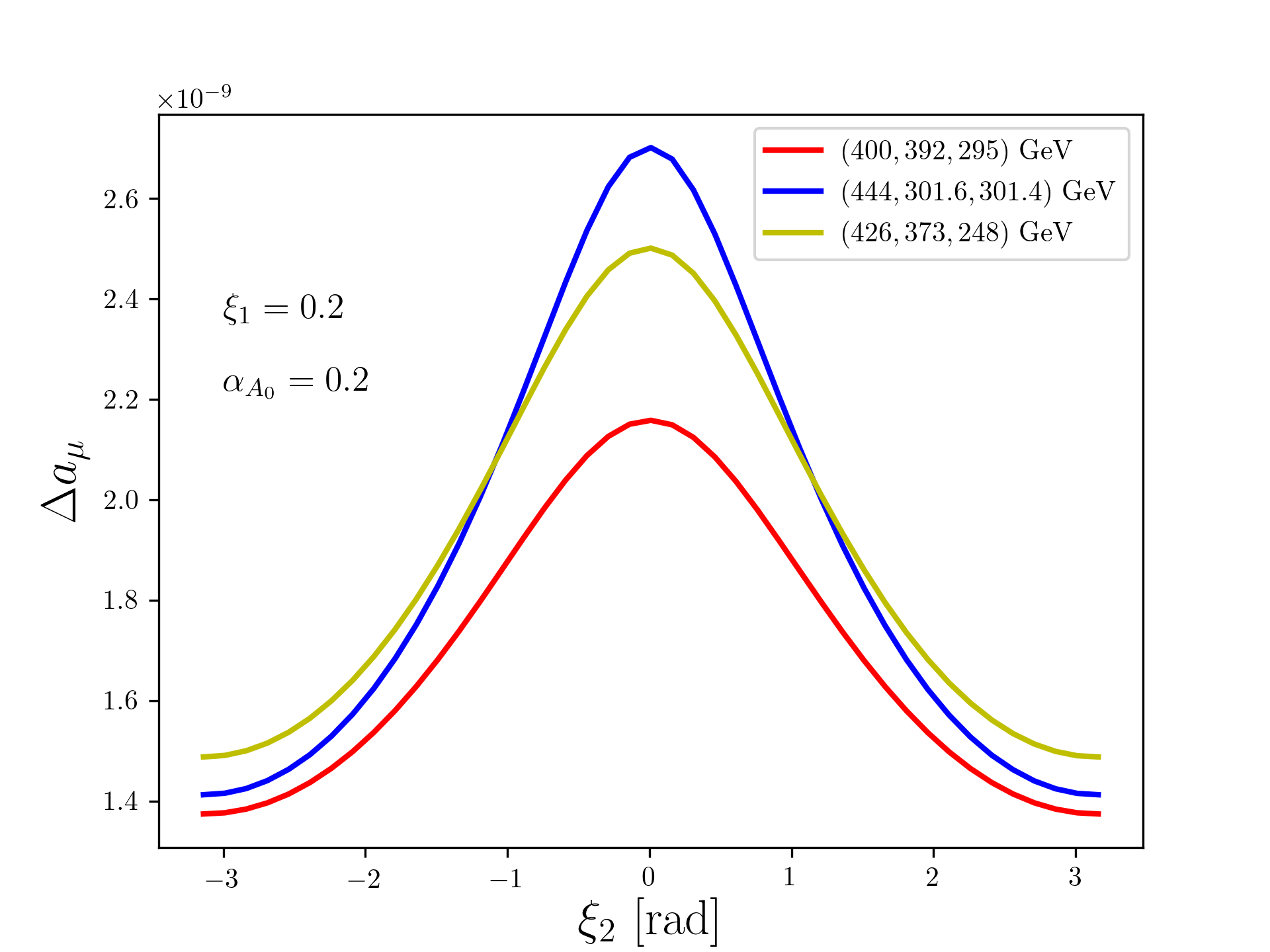
Figure 12: Top and middle panels: Exclusion plots in the CP phases $\xi_{1}$ and $\xi_{2}$ arising from the $\Delta{a^{\rm FB}_{\mu}}$ constraint. The contours correspond to $\Delta a_{\mu}\times 10^{9}$ consistent with the combined experimental result on $g-2$. Bottom panel: Variation of $a^{\rm SUSY}_{\mu}$ with the phase $\xi_{2}$. In all plots, $\alpha_{A_{0}}=0.2$ rad. The masses of the light particles in the loops are in this order $(\tilde{\mu},\tilde{\chi}^{\pm}_{1},\tilde{\chi}^{0}_{1})$: $(400,392,1,391.7)$ GeV for the top panel and $(445,301.6,301.4)$ GeV for the middle panel and shown in the legend for the bottom panel. The star in the top and middle panels indicate illustrative tiny regions of the cancellation mechanism Ibrahim:1998je where one can simultaneously obtain a muon $g-2$ and the electron EDM consistent with experiment, $|d_{e}|<1.1\times 10^{-29}e$cm.

The top panels of Fig. 12 show the excluded regions (shaded) in the $\xi_{1}$-$\xi_{2}$ plane due to the $\Delta{a^{\rm FB}_{\mu}}$ constraint for two points chosen from the large set of points obtained from the scan. The contours shown in the allowed regions correspond to $\Delta a_{\mu}$ consistent with the combined Brookhaven and Fermilab results. The lower panel shows the sensitivity of $\Delta a_{\mu}$ to the CP phase $\xi_{2}$ with a range of values consistent with the recent $(g-2)_{\mu}$ experiment. We note here that in addition to the constraint on the CP phases by the $(g-2)_{\mu}$ experiment, the phases are also subject to the EDM constraints. Thus while the phases satisfying the EDM constraints must lie in the white regions of the upper two panels of Fig. 12, the EDM constraints on them are much stronger, the strongest being the electron EDM which has the upper limit of $|d_{e}|<1.1\times 10^{-29}e$cm. For models with low slepton mass spectrum, which is the case here, a satisfaction of the EDM constraint can come about via the cancellation mechanism Ibrahim:1998je in tiny regions of the parameter space. An illustration of this phenomenon is given in the upper two panels of Fig. 12 where we display two tiny regions of the parameter space where the electron EDM constraint is satisfied.

VII 7. Conclusion

In this work we have shown that the combined Fermilab and Brookhaven data on $a^{\rm exp}_{\mu}-a^{\rm SM}_{\mu}$ has important implications for the discovery of supersymmetry at HL-LHC and HE-LHC. Specifically, exploration of the SUGRA parameter space using machine learning shows that the combined Fermilab and Brookhaven $\Delta{a^{\rm FB}_{\mu}}$ constraint indicates that the favored region of the parameter space is that of $\tilde{g}$SUGRA where gluino-driven radiative breaking of the electroweak symmetry occurs. In this region the renormalization group analysis leads to a split light and heavy mass spectrum where the electroweak gauginos and the sleptons are light lying in the few hundred GeV range, while the remaining mass spectrum is heavy. The light spectrum which includes the neutralino, the chargino, the smuon, and the smuon-neutrino can produce a correction to the muon anomaly consistent with $\Delta{a^{\rm FB}_{\mu}}$. Further, the light stau and the chargino are seen to be the lightest charged particles while the sleptons are light enough to be prime candidates for discovery at HL-LHC and HE-LHC. We perform a signal region analysis and compute the integrated luminosity needed for SUSY discovery. It is shown that supergravity models which produce a correction to $\Delta a^{\rm SM}_{\mu}$ of size indicated $\Delta{a^{\rm FB}_{\mu}}$ are discoverable at HL-LHC within the optimal integrated luminosity and with a smaller integrated luminosity at HE-LHC. It is also shown that $\Delta{a^{\rm FB}_{\mu}}$ puts constraints on the CP phases that enter the muon anomaly and eliminates significant regions of their parameter space. These constraints are independent of the EDM constraints which must be imposed in the regions of CP phases allowed by the muon anomalous magnetic moment. Finally we note here some previous and recent works related to the $g-2$ anomaly works .

- (1) B. Abi et al. [Muon g-2], Phys. Rev. Lett. 126, no.14, 141801 (2021) doi:10.1103/PhysRevLett.126.141801 [arXiv:2104.03281 [hep-ex]].
- (2) G. W. Bennett et al. [Muon g-2], Phys. Rev. D 73, 072003 (2006) doi:10.1103/PhysRevD.73.072003 [arXiv:hep-ex/0602035 [hep-ex]].
- (3) M. Tanabashi, et al., Review of Particle Physics, Phys. Rev. D98 (3) (2018) 030001. doi:10.1103/PhysRevD.98. 030001
- (4) T. Aoyama, N. Asmussen, M. Benayoun, J. Bijnens, T. Blum, M. Bruno, I. Caprini, C. M. Carloni Calame, M. Cè and G. Colangelo, et al. Phys. Rept. 887, 1-166 (2020) doi:10.1016/j.physrep.2020.07.006 [arXiv:2006.04822 [hep-ph]].
- (5) S. Borsanyi, Z. Fodor, J. N. Guenther, C. Hoelbling, S. D. Katz, L. Lellouch, T. Lippert, K. Miura, L. Parato and K. K. Szabo, et al. Nature 593, no.7857, 51-55 (2021) doi:10.1038/s41586-021-03418-1 [arXiv:2002.12347 [hep-lat]].
- (6) K. Fujikawa, B. W. Lee, and A. I. Sanda, Phys. Rev. D6, 2923 (1972); R. Jackiw and S. Weinberg, Phys. Rev. D5, 2473 (1972); G. Altarelli, N. Cabbibo, and L. Maiani, Phys. Lett. B40, 415 (1972); I. Bars and M. Yoshimura, Phys. Rev. D6, 374 (1972); W. A. Bardeen, R. Gastmans, and B. E. Lautrup, Nucl. Phys. B46, 315 (1972).
- (7) A. Czarnecki, B. Krause and W. J. Marciano, Phys. Rev. Lett. 76, 3267-3270 (1996) doi:10.1103/PhysRevLett.76.3267 [arXiv:hep-ph/9512369 [hep-ph]].
- (8) D. A. Kosower, L. M. Krauss and N. Sakai, Phys. Lett. B 133, 305-310 (1983) doi:10.1016/0370-2693(83)90152-1
- (9) T. C. Yuan, R. L. Arnowitt, A. H. Chamseddine and P. Nath, Z. Phys. C 26, 407 (1984) doi:10.1007/BF01452567
- (10) J. L. Lopez, D. V. Nanopoulos and X. Wang, Phys. Rev. D 49, 366-372 (1994) doi:10.1103/PhysRevD.49.366 [arXiv:hep-ph/9308336 [hep-ph]].
- (11) U. Chattopadhyay and P. Nath, Phys. Rev. D 53, 1648-1657 (1996) doi:10.1103/PhysRevD.53.1648 [arXiv:hep-ph/9507386 [hep-ph]].
- (12) T. Moroi, Phys. Rev. D 53, 6565-6575 (1996) [erratum: Phys. Rev. D 56, 4424 (1997)] doi:10.1103/PhysRevD.53.6565 [arXiv:hep-ph/9512396 [hep-ph]].
- (13) M. Carena, G. F. Giudice and C. E. M. Wagner, Phys. Lett. B 390, 234-242 (1997) doi:10.1016/S0370-2693(96)01396-2 [arXiv:hep-ph/9610233 [hep-ph]].
- (14) A. Czarnecki and W. J. Marciano, Phys. Rev. D 64, 013014 (2001) doi:10.1103/PhysRevD.64.013014 [arXiv:hep-ph/0102122 [hep-ph]].
- (15) U. Chattopadhyay and P. Nath, Phys. Rev. Lett. 86, 5854-5857 (2001) doi:10.1103/PhysRevLett.86.5854 [arXiv:hep-ph/0102157 [hep-ph]].
- (16) L. L. Everett, G. L. Kane, S. Rigolin and L. T. Wang, Phys. Rev. Lett. 86, 3484-3487 (2001) doi:10.1103/PhysRevLett.86.3484 [arXiv:hep-ph/0102145 [hep-ph]].
- (17) J. L. Feng and K. T. Matchev, Phys. Rev. Lett. 86, 3480-3483 (2001) doi:10.1103/PhysRevLett.86.3480 [arXiv:hep-ph/0102146 [hep-ph]].
- (18) E. A. Baltz and P. Gondolo, Phys. Rev. Lett. 86, 5004 (2001) doi:10.1103/PhysRevLett.86.5004 [arXiv:hep-ph/0102147 [hep-ph]].
- (19) S. Chatrchyan et al. [CMS], Phys. Lett. B 716, 30-61 (2012) doi:10.1016/j.physletb.2012.08.021 [arXiv:1207.7235 [hep-ex]].
- (20) G. Aad et al. [ATLAS], Phys. Lett. B 716, 1-29 (2012) doi:10.1016/j.physletb.2012.08.020 [arXiv:1207.7214 [hep-ex]].
- (21) S. Akula, B. Altunkaynak, D. Feldman, P. Nath and G. Peim, Phys. Rev. D 85, 075001 (2012) doi:10.1103/PhysRevD.85.075001 [arXiv:1112.3645 [hep-ph]].
- (22) A. Arbey, M. Battaglia, A. Djouadi, F. Mahmoudi and J. Quevillon, Phys. Lett. B 708, 162 (2012); H. Baer, V. Barger and A. Mustafayev, Phys. Rev. D 85, 075010 (2012); J. Ellis and K. A. Olive, Eur. Phys. J. C 72, 2005 (2012); S. Heinemeyer, O. Stal and G. Weiglein, Phys. Lett. B 710, 201 (2012);
- (23) A. H. Chamseddine, R. Arnowitt and P. Nath, Phys. Rev. Lett. 49 (1982) 970; P. Nath, R. L. Arnowitt and A. H. Chamseddine, Nucl. Phys. B 227, 121 (1983); L. J. Hall, J. D. Lykken and S. Weinberg, Phys. Rev. D 27, 2359 (1983). doi:10.1103/PhysRevD.27.2359
- (24) J. Hollingsworth, M. Ratz, P. Tanedo and D. Whiteson, [arXiv:2103.06957 [hep-th]].
- (25) C. Balázs et al. [DarkMachines High Dimensional Sampling Group], JHEP 05, 108 (2021) doi:10.1007/JHEP05(2021)108 [arXiv:2101.04525 [hep-ph]].
- (26) S. Akula and P. Nath, Phys. Rev. D 87, no.11, 115022 (2013) doi:10.1103/PhysRevD.87.115022 [arXiv:1304.5526 [hep-ph]].
- (27) A. Aboubrahim and P. Nath, Phys. Rev. D 100, no.1, 015042 (2019) doi:10.1103/PhysRevD.100.015042 [arXiv:1905.04601 [hep-ph]].
- (28) A. Aboubrahim, P. Nath and R. M. Syed, JHEP 01, 047 (2021) doi:10.1007/JHEP01(2021)047 [arXiv:2005.00867 [hep-ph]].
- (29) J. R. Ellis, K. Enqvist, D. V. Nanopoulos and K. Tamvakis, Phys. Lett. B 155, 381-386 (1985) doi:10.1016/0370-2693(85)91591-6
- (30) A. Corsetti and P. Nath, Phys. Rev. D 64, 125010 (2001); A. Birkedal-Hansen and B. D. Nelson, Phys. Rev. D 67, 095006 (2003); G. Belanger, F. Boudjema, A. Cottrant, A. Pukhov and A. Semenov, Nucl. Phys. B 706, 411 (2005); H. Baer, A. Mustafayev, E. K. Park, S. Profumo and X. Tata, JHEP 04 (2006), 041 doi:10.1088/1126-6708/2006/04/041 [arXiv:hep-ph/0603197 [hep-ph]]; I. Gogoladze, F. Nasir, Q. Shafi and C. S. Un, Phys. Rev. D 90, no. 3, 035008 (2014) doi:10.1103/PhysRevD.90.035008; S. P. Martin, Phys. Rev. D 79, 095019 (2009) doi:10.1103/PhysRevD.79.095019
- (31) D. Feldman, Z. Liu and P. Nath, Phys. Rev. D 80, 015007 (2009) doi:10.1103/PhysRevD.80.015007 [arXiv:0905.1148 [hep-ph]].
- (32) A. S. Belyaev, S. F. King and P. B. Schaefers, Phys. Rev. D 97, no.11, 115002 (2018) doi:10.1103/PhysRevD.97.115002 [arXiv:1801.00514 [hep-ph]].
- (33) S. Heinemeyer, D. Stockinger and G. Weiglein, Nucl. Phys. B 690, 62-80 (2004) doi:10.1016/j.nuclphysb.2004.04.017 [arXiv:hep-ph/0312264 [hep-ph]].
- (34) F. Staub, [arXiv:1906.03277 [hep-ph]].
- (35) W. Porod, Comput. Phys. Commun. 153, 275-315 (2003) doi:10.1016/S0010-4655(03)00222-4 [arXiv:hep-ph/0301101 [hep-ph]].
- (36) W. Porod and F. Staub, Comput. Phys. Commun. 183, 2458-2469 (2012) doi:10.1016/j.cpc.2012.05.021 [arXiv:1104.1573 [hep-ph]].
- (37) G. Bélanger, F. Boudjema, A. Pukhov and A. Semenov, Comput. Phys. Commun. 192, 322-329 (2015) doi:10.1016/j.cpc.2015.03.003 [arXiv:1407.6129 [hep-ph]].
- (38) J. Bernon and B. Dumont, Eur. Phys. J. C 75, no.9, 440 (2015) doi:10.1140/epjc/s10052-015-3645-9 [arXiv:1502.04138 [hep-ph]].
- (39) S. Kraml, T. Q. Loc, D. T. Nhung and L. Ninh, SciPost Phys. 7, no.4, 052 (2019) doi:10.21468/SciPostPhys.7.4.052 [arXiv:1908.03952 [hep-ph]].
- (40) P. Bechtle, S. Heinemeyer, O. Stål, T. Stefaniak and G. Weiglein, Eur. Phys. J. C 74, no.2, 2711 (2014) doi:10.1140/epjc/s10052-013-2711-4 [arXiv:1305.1933 [hep-ph]].
- (41) P. Bechtle, D. Dercks, S. Heinemeyer, T. Klingl, T. Stefaniak, G. Weiglein and J. Wittbrodt, Eur. Phys. J. C 80, no.12, 1211 (2020) doi:10.1140/epjc/s10052-020-08557-9 [arXiv:2006.06007 [hep-ph]].
- (42) C. K. Khosa, S. Kraml, A. Lessa, P. Neuhuber and W. Waltenberger, doi:10.31526/lhep.2020.158 [arXiv:2005.00555 [hep-ph]].
- (43) S. Kraml, S. Kulkarni, U. Laa, A. Lessa, W. Magerl, D. Proschofsky-Spindler and W. Waltenberger, Eur. Phys. J. C 74, 2868 (2014) doi:10.1140/epjc/s10052-014-2868-5 [arXiv:1312.4175 [hep-ph]].
- (44) S. Kraml, S. Kulkarni, U. Laa, A. Lessa, V. Magerl, W. Magerl, D. Proschofsky-Spindler, M. Traub and W. Waltenberger, [arXiv:1412.1745 [hep-ph]].
- (45) D. Barducci, G. Belanger, J. Bernon, F. Boudjema, J. Da Silva, S. Kraml, U. Laa and A. Pukhov, Comput. Phys. Commun. 222, 327-338 (2018) doi:10.1016/j.cpc.2017.08.028 [arXiv:1606.03834 [hep-ph]].
- (46) A. Aboubrahim, T. Ibrahim and P. Nath, Phys. Rev. D 94, no.1, 015032 (2016) doi:10.1103/PhysRevD.94.015032 [arXiv:1606.08336 [hep-ph]].
- (47) P. Athron, M. Bach, H. G. Fargnoli, C. Gnendiger, R. Greifenhagen, J. h. Park, S. Paßehr, D. Stöckinger, H. Stöckinger-Kim and A. Voigt, Eur. Phys. J. C 76, no.2, 62 (2016) doi:10.1140/epjc/s10052-015-3870-2 [arXiv:1510.08071 [hep-ph]].
- (48) C. Macolino [DARWIN], J. Phys. Conf. Ser. 1468, no.1, 012068 (2020) doi:10.1088/1742-6596/1468/1/012068
- (49) A. Buckley, Eur. Phys. J. C 75, no.10, 467 (2015) doi:10.1140/epjc/s10052-015-3638-8 [arXiv:1305.4194 [hep-ph]].
- (50) J. Debove, B. Fuks and M. Klasen, Nucl. Phys. B 849, 64-79 (2011) doi:10.1016/j.nuclphysb.2011.03.015 [arXiv:1102.4422 [hep-ph]].
- (51) B. Fuks, M. Klasen, D. R. Lamprea and M. Rothering, Eur. Phys. J. C 73, 2480 (2013) doi:10.1140/epjc/s10052-013-2480-0 [arXiv:1304.0790 [hep-ph]].
- (52) J. Alwall, R. Frederix, S. Frixione, V. Hirschi, F. Maltoni, O. Mattelaer, H. S. Shao, T. Stelzer, P. Torrielli and M. Zaro, JHEP 07, 079 (2014) doi:10.1007/JHEP07(2014)079 [arXiv:1405.0301 [hep-ph]].
- (53) A. Buckley, J. Ferrando, S. Lloyd, K. Nordström, B. Page, M. Rüfenacht, M. Schönherr and G. Watt, Eur. Phys. J. C 75, 132 (2015) doi:10.1140/epjc/s10052-015-3318-8 [arXiv:1412.7420 [hep-ph]].
- (54) T. Sjöstrand, S. Ask, J. R. Christiansen, R. Corke, N. Desai, P. Ilten, S. Mrenna, S. Prestel, C. O. Rasmussen and P. Z. Skands, Comput. Phys. Commun. 191, 159-177 (2015) doi:10.1016/j.cpc.2015.01.024 [arXiv:1410.3012 [hep-ph]].
- (55) M. Cacciari, G. P. Salam and G. Soyez, Eur. Phys. J. C 72, 1896 (2012) doi:10.1140/epjc/s10052-012-1896-2 [arXiv:1111.6097 [hep-ph]].
- (56) M. Cacciari, G. P. Salam and G. Soyez, JHEP 04, 063 (2008) doi:10.1088/1126-6708/2008/04/063 [arXiv:0802.1189 [hep-ph]].
- (57) J. de Favereau et al. [DELPHES 3], JHEP 02, 057 (2014) doi:10.1007/JHEP02(2014)057 [arXiv:1307.6346 [hep-ex]].
- (58) P. Speckmayer, A. Hocker, J. Stelzer and H. Voss, J. Phys. Conf. Ser. 219, 032057 (2010) doi:10.1088/1742-6596/219/3/032057
- (59) I. Antcheva, M. Ballintijn, B. Bellenot, M. Biskup, R. Brun, N. Buncic, P. Canal, D. Casadei, O. Couet and V. Fine, et al. Comput. Phys. Commun. 182, 1384-1385 (2011) doi:10.1016/j.cpc.2011.02.008
- (60) C. G. Lester and D. J. Summers, Phys. Lett. B 463, 99-103 (1999) doi:10.1016/S0370-2693(99)00945-4 [arXiv:hep-ph/9906349 [hep-ph]].
- (61) A. Barr, C. Lester and P. Stephens, J. Phys. G 29, 2343-2363 (2003) doi:10.1088/0954-3899/29/10/304 [arXiv:hep-ph/0304226 [hep-ph]].
- (62) C. G. Lester and B. Nachman, JHEP 03, 100 (2015) doi:10.1007/JHEP03(2015)100 [arXiv:1411.4312 [hep-ph]].
- (63) G. Aad et al. [ATLAS], Eur. Phys. J. C 80, no.2, 123 (2020) doi:10.1140/epjc/s10052-019-7594-6 [arXiv:1908.08215 [hep-ex]].
- (64) X. Cid Vidal, M. D’Onofrio, P. J. Fox, R. Torre, K. A. Ulmer, A. Aboubrahim, A. Albert, J. Alimena, B. C. Allanach and C. Alpigiani, et al. CERN Yellow Rep. Monogr. 7, 585-865 (2019) doi:10.23731/CYRM-2019-007.585 [arXiv:1812.07831 [hep-ph]].
- (65) M. Cepeda, S. Gori, P. Ilten, M. Kado, F. Riva, R. Abdul Khalek, A. Aboubrahim, J. Alimena, S. Alioli and A. Alves, et al. CERN Yellow Rep. Monogr. 7, 221-584 (2019) doi:10.23731/CYRM-2019-007.221 [arXiv:1902.00134 [hep-ph]].
- (66) A. Aboubrahim and P. Nath, Phys. Rev. D 96, no.7, 075015 (2017) doi:10.1103/PhysRevD.96.075015 [arXiv:1708.02830 [hep-ph]].
- (67) A. Aboubrahim and P. Nath, Phys. Rev. D 98, no.1, 015009 (2018) doi:10.1103/PhysRevD.98.015009 [arXiv:1804.08642 [hep-ph]].
- (68) T. Ibrahim and P. Nath, Phys. Rev. D 62, 015004 (2000) doi:10.1103/PhysRevD.62.015004 [arXiv:hep-ph/9908443 [hep-ph]].
- (69) T. Ibrahim, U. Chattopadhyay and P. Nath, Phys. Rev. D 64, 016010 (2001) doi:10.1103/PhysRevD.64.016010 [arXiv:hep-ph/0102324 [hep-ph]].
- (70) T. Ibrahim and P. Nath, Phys. Rev. D 58, 111301 (1998) [erratum: Phys. Rev. D 60, 099902 (1999)] doi:10.1103/PhysRevD.58.111301 [arXiv:hep-ph/9807501 [hep-ph]].
- (71) E. Kiritsis and P. Anastasopoulos, JHEP 05, 054 (2002) doi:10.1088/1126-6708/2002/05/054 [arXiv:hep-ph/0201295 [hep-ph]]; J. Cao, Z. Heng, D. Li and J. M. Yang, Phys. Lett. B 710, 665-670 (2012) doi:10.1016/j.physletb.2012.03.052 [arXiv:1112.4391 [hep-ph]]; N. Chen, B. Wang and C. Y. Yao, [arXiv:2102.05619 [hep-ph]]; D. Sabatta, A. S. Cornell, A. Goyal, M. Kumar, B. Mellado and X. Ruan, Chin. Phys. C 44, no.6, 063103 (2020) doi:10.1088/1674-1137/44/6/063103 [arXiv:1909.03969 [hep-ph]].