Effective bath model for arrays of coupled non-Hermitian nanoresonators

Abstract

Nanophotonics systems have recently been studied under the perspective of non-Hermitian physics. Given their potential for wavefront control, nonlinear optics and quantum optics, it is crucial to develop predictive tools to assist their design. We present here a simple model relying on the coupling to an effective bath consisting of a continuum of modes to describe systems of coupled resonators, and test it on dielectric nanocylinder chains accessible to experiments. The effective coupling constants, which depend non-trivially on the distance between resonators, are extracted from numerical simulations in the case of just two coupled elements. The model predicts successfully the dispersive and reactive nature of modes for configurations with multiple resonators, as validated by numerical solutions. It can be applied to larger systems, which are hardly solvable with finite-element approaches.

I Introduction

Nanophotonics deals with light behavior at nanoscopic scale, and encompasses plasmonics [1, 2], photonic crystals [3, 4], and metamaterial optics [5, 6, 7, 8, 9]. While light confinement is a central challenge for these domains [8, 9, 10, 11], conceiving or exploring low quality factor (Q) systems is not always straightforward, as scattering or dissipative processes are omnipresent. In the past decade, nanophotonics has greatly benefited from non-Hermitian physics [12, 13], which corresponds to the study of either time-dependent Schrödinger equations or time-independent Schrödinger equations with operators that are not Hermitian [14, 15]. Those non-Hermitian terms describe dissipative processes such as the interaction with the environment. Non-Hermitian approaches have already been adopted in plasmonics [16, 12, 13] and more recently their dielectric counterparts [17] have also drawn a growing interest for conceiving novel miniaturized optical devices for wavefront shaping [7, 18], harmonic generation [19, 8, 10] and quantum photonics [20].

In this work, we theoretically study one-dimensional (1D) chains of $N$ dissipative dielectric nanoresonators by using an analytical non-Hermitian quantum model. Our approach is to feed the model with complex coupling parameters obtained from a numerical simulation in the case $N=2$, and then validate it with longer chains by comparison with brute-force calculations. It thereby becomes a predictive tool, essential for overcoming numerical limitations associated to the study and design of larger systems of interest. This model includes both direct coupling between resonators and coupling mediated by the electromagnetic continuum acting as a reservoir. Such couplings are determined by fitting the numerical solution of Maxwell’s equations in the case of two coupled resonators. The latter is obtained via finite-element-method (FEM) simulations on our trial system, which consists of chains of equidistant Aluminum Gallium Arsenide (AlGaAs) nanocylinders along $x$ [Fig. 1(a)]. Their size determines the spatial and spectral properties of their eigenmodes [21, 22]. The numerical integration domain is bounded by a perfectly matched layer (PML) that suppresses spurious electromagnetic-field reflection at the edges of the integration domain. We focus on the hybrid modes stemming from from magnetic dipoles (MDs) of single nanocylinders (see more details in supplementary material). Their radius and height are set at 300 nm and 400 nm respectively, to lift the spectral degeneracy between out-of-plane (MD_z) and in-plane (MD_x and MD_y) magnetic dipolar modes, the coupling strength being dictated by the gap $d$ between the nanocylinders. Figure 1(b,c) displays $N=2$ chain spectra for hybrid MD_x and MD_z as a function of the gap. A pair of bonding and antibonding modes is formed, corresponding to two complex eigenfrequencies in phase opposition. In the following, we will neglect the coupling between two MDs oriented along different directions, since the field overlap between two non-collinear MDs is 3 orders of magnitude smaller than the one between two collinear MDs. We identify two coupling regimes: an exponential-like decay of the frequency splitting for small gaps; and a pseudo-periodic variation of the complex eigenfrequencies for larger gaps. Outside each leaky resonator, the electromagnetic field decreases much slower than for high-Q systems like micropillars [23] or whispering gallery mode resonators [24, 25, 26, 27]. When more than one resonator is involved, the corresponding eigenfrequencies oscillate and result in non-zero energy splitting. A good figure of merit to assess the range of this interaction is the scattering cross-section of each resonator mode, which can be as large as ten times the cylinder cross-section in the case of MD [21, 17]. The eigenfrequency spectra of a pair of MD eigenmodes exhibit degeneracy points which occur at different gap values for real and imaginary parts and depend on the specific mode. This feature has already been reported recently [28] and offers interesting perspectives for meta-optics design and band engineering. Additionally, the coupling between MDs modifies the quality factor of those modes. For a single AlGaAs nanocylinder of the same dimensions, the Q factor of the MD_z is 7 and that the MD_x and MD_y is 5.5: our simulations thus confirm that even long-range coupling between nanoresonators can increase Q factor, although light remains poorly confined in those structures, which justifies the introduction of a non-Hermitian formalism.

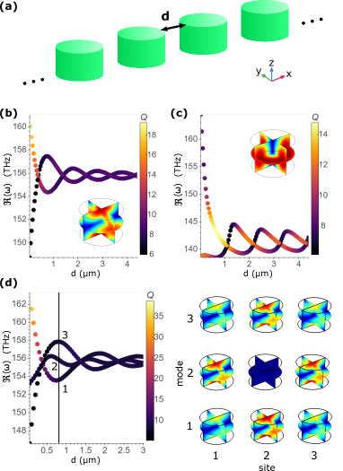
Figure 1: AlGaAs nanocylinder ensembles and numerical simulations for short chains. (a): schematic of the system. The gap denotes edge-to-edge distance between nanocylinders. (b) and (c): numerical simulation for $N=2$: real part of the eigenfrequency $\omega$ as a function of gap for MD_x and MD_z respectively, with colorbar providing the quality factor $Q=\Re(\omega)/2\Im(\omega)$. Inset: 3D plot of the electric field norm in a nanocylinder. (d) case $N=3$ for MD_x. Electric field norm inside nanocylinders for each mode for a gap of $0.75~{}\rm{$\mathrm{\SIUnitSymbolMicro m}$}$. Normalized powers inside the resonators for each mode are 1: (0.27, 0.47, 0.26); 2: (0.50, 0, 0.50); 3: (0.22, 0.56, 0.22).

II Non-Hermitian quantum formalism

To describe the dynamics of an ensemble of leaky resonators, let us consider an Hamiltonian consisting of a tight-binding term for the nanoresonators coupled to an effective bath. The non-Hermitian character is obtained by tracing out the bath degrees of freedom. Our basic idea is to extract the effective bath parameters from exact FEM results for two coupled resonators, and then use the formalism to predict the modes for an arbitrary number and arrangement of nanoresonators. In the rotating-wave approximation, the Hamiltonian reads (with $\hbar=1$):

$$\hat{H}= \hat{H}_{\rm{sys}}+\hat{H}_{\rm{bath}}+\hat{H}_{\rm{int}},$$ (1)

$$\hat{H}_{\rm{sys}}= \sum_{j}\omega_{j}\hat{a}_{j}^{\dagger}\hat{a}_{j}+\sum_{j,j^{\prime}}J(d_{jj^{\prime}})(\hat{a}_{j}^{\dagger}\hat{a}_{j^{\prime}}+\mathrm{h.c.}),$$ (2)

$$\hat{H}_{\rm{bath}}= \int\mathrm{d}\eta~{}\omega_{\eta}\hat{\alpha}_{\eta}^{\dagger}\hat{\alpha}_{\eta},$$ (3)

$$\hat{H}_{\rm{int}}= \sum_{j}\int\mathrm{d}\eta~{}\mathrm{i}(g_{j\eta}\hat{a}_{j}^{\dagger}\hat{\alpha}_{\eta}-g_{j\eta}^{*}\hat{\alpha}_{\eta}^{\dagger}\hat{a}_{j}).$$ (4)

$\hat{H}_{\rm{sys}}$ is the bare resonators’ Hamiltonian, where each nanoresonator has one mode with annihilation operator $\hat{a}_{j}$ and frequency $\omega_{j}$, $j$ and $j^{\prime}$ denoting different resonators. In the following, we will consider equally spaced identical resonators ($\omega_{j}=\omega_{0}$, $d_{jj^{\prime}}=d$). $J(d)$ describes the coherent coupling between two resonators via evanescent field, and is essentially determined by the distance $d$ between them for a given set of resonators. The second term $\hat{H}_{\rm{bath}}$ describes the continuum of radiation modes represented by the annihilation operators $\hat{\alpha}_{\eta}$ indexed by $\eta$, and $\hat{H}_{\rm{int}}$ is the interaction Hamiltonian between the system and the bath, where $g_{j\eta}$ is the coupling between the $j^{th}$ nanoresonator and the radiation mode $\hat{\alpha}_{\eta}$. The operators $\hat{a}_{j}$ and $\hat{\alpha}_{\eta}$ obey bosonic commutation relations, i.e. $[\hat{a}_{j},\hat{a}^{\dagger}_{j^{\prime}}]=\delta_{jj^{\prime}}$ and $[\hat{\alpha}_{\eta},\hat{\alpha}^{\dagger}_{\eta^{\prime}}]=\delta(\eta-\eta^{\prime})$. All commutators between $\hat{a}_{j}$ or $\hat{a}^{\dagger}_{j}$ and $\hat{\alpha}_{\eta}$ or $\hat{\alpha}^{\dagger}_{\eta}$ are taken to be zero. In the Heisenberg picture, one can derive the quantum Langevin equation [29] (see Supplementary Material for the derivation) for $\hat{a}_{j}$:

$$\dfrac{\mathrm{d}\hat{a}_{j}}{\mathrm{d}t}=-\mathrm{i}\left[\omega_{0}\hat{a}_{j}+J(d)\sum_{j^{\prime}}\hat{a}_{j^{\prime}}\right]-\sum_{k}\int_{-\infty}^{\infty}\mathrm{d}t^{\prime}\Gamma_{jk}(t-t^{\prime})\hat{a}_{k}(t^{\prime})+\hat{F}_{j}(t),$$ (5)

where we have defined the damping kernel $\Gamma_{jk}(\tau)=\Theta(\tau)\int\mathrm{d}\eta~{}g_{j\eta}g_{k\eta}^{*}e^{-\mathrm{i}\omega_{\eta}\tau}$ and the Langevin force $\hat{F}_{j}(t)=\int\mathrm{d}\eta~{}g_{j\eta}e^{-\mathrm{i}\omega_{\eta}(t-t_{0})}\hat{\alpha}_{\eta}(t_{0})$ where $t_{0}\rightarrow-\infty$.

After applying Fourier transform, adopting the convention $\tilde{A}(\omega)=\int_{-\infty}^{\infty}\mathrm{d}te^{\mathrm{i}\omega t}A(t)$, to Eq. (5), we obtain the equations in the frequency domain:

$$\omega\tilde{a}_{j}(\omega)=\omega_{0}\tilde{a}_{j}(\omega)+J(d)\sum_{j^{\prime}}\tilde{a}_{j^{\prime}}(\omega)-\mathrm{i}\sum_{k}\tilde{\Gamma}_{jk}(\omega)\tilde{a}_{k}(\omega)+\mathrm{i}\tilde{F}_{j}(\omega),$$ (6)

which can be cast into the following matrix form

$$\mathcal{M}(\omega,d)\begin{bmatrix}\tilde{a}_{1}(\omega)\\ \vdots\\ \tilde{a}_{N}(\omega)\end{bmatrix}+\mathrm{i}\begin{bmatrix}\tilde{F}_{1}(\omega)\\ \vdots\\ \tilde{F}_{N}(\omega)\end{bmatrix}=0,$$ (7)

with eigenvalues $\lambda^{(i)}$ that can be obtained by diagonalization. We can then solve for the resonant frequencies

$$\Omega_{\text{res}}=\left\{\omega_{i}^{\star}\in\mathbb{R}~{}|~{}\exists i,~{}\omega_{i}^{\star}=\operatorname*{arg\,min}_{\omega}|\lambda^{(i)}(\omega)|^{2}\right\},$$ (8)

which, by definition, give local maxima of the amplitude of the frequency response, and the corresponding damping

$$\gamma_{i}^{\star}=-\Im[\lambda^{(i)}(\omega_{i}^{\star})].$$ (9)

For a compact notation, we can assign the complex frequency to the resonant mode $\omega^{\text{res}}_{i}=\omega^{\star}_{i}-\mathrm{i}\gamma_{i}^{\star}$. In the case $N=2$, with identical resonators, the matrix can be explicitly written as :

$$\mathcal{M}(\omega,d)=\begin{bmatrix}\omega_{0}-\omega-\mathrm{i}\tilde{\Gamma}_{\rm{diag}}(\omega,d)&J(d)-\mathrm{i}\tilde{\Gamma}_{\rm{off}}(\omega,d)\\ J(d)-\mathrm{i}\tilde{\Gamma}_{\rm{off}}(\omega,d)&\omega_{0}-\omega-\mathrm{i}\tilde{\Gamma}_{\rm{diag}}(\omega,d)\end{bmatrix}$$ (10)

where we have further assumed $\tilde{\Gamma}_{11}=\tilde{\Gamma}_{22}:=\tilde{\Gamma}_{\rm{diag}}$ and $\tilde{\Gamma}_{12}=\tilde{\Gamma}_{21}:=\tilde{\Gamma}_{\text{off}}$ by symmetry.

The coupling functions $J$, $\tilde{\Gamma}_{\rm{diag}}$ and $\tilde{\Gamma}_{\rm{off}}$ can be fitted from the simulation results presented in Fig. 1. To simplify the treatment, we expand them to first order in $\omega$, which allows us to determine a set of possible reservoir functions from the simulation of the $N=2$ system (see supplementary material for a detailed derivation). For an $N$-resonator chain, the matrix in Eq. (7) can be written as:

$$\mathcal{M}_{N}(\omega,d)=(\omega-\omega_{0})I(N)+J(d)Sec(N)-\mathrm{i}\big{(}\tilde{\Gamma}_{jk}(\omega,d)\big{)}_{\{j,k\}\in\llbracket 1;N\rrbracket^{2}}$$ (11)

with $I(N)$ being the $N\times N$ identity matrix, and $Sec(N)$ the $N\times N$ secondary diagonal matrix.

III Results and discussion

The same model is used to predict the modes in the presence of three resonators [Fig. 2(a) solid blue line] and four resonators [Fig. 2(c) solid blue line], using only what we learned from the $N=2$ case behavior as a function of the gap. The main features of the fully numerical simulations are captured by our model: exponential-like decay, pseudo periodicity, and degeneracy points of both imaginary and real parts of the eigenfrequencies. All this confirms that a relatively simple analytical non-Hermitian formalism can predict the physics of non-trivial nanophotonic systems.

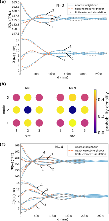
Figure 2: Comparison between the analytical model and the FEM simulations. (a) Case $N=3$: real part (top panel) and imaginary part (bottom panel) of the eigenfrequency $\omega$ as a function of gap for MD_x. (b) Probability density map in the case $N=3$, depending if next-nearest neighbor coupling is implemented (right, NNN) or not (left, NN). Modes are labelled according to Fig. 1(d). (c) Case $N=4$: real part (top panel) and imaginary part (bottom panel) of the eigenfrequency $\omega$ as a function of gap for MD_x.

Strikingly, degeneracy points for real parts on one hand, and for imaginary parts on the other hand, arise for the same gaps in the cases $N=2$, $3$ and $4$. The fact that they are independent of $N$ indicates that they only depend on single resonator’s characteristics. The numerical spectra of the eigenmodes in the cases $N=3$ and $4$ are fairly described by our formalism (see the relative error in the Fig. S4 of the supplementary material). Furthermore, following the correspondence between the probability density and the power stored inside each resonator, the eigenmodes solution of the non-unitary dynamics in the case $N=3$ [Fig. 2(b)] displays more symmetric results than the FEM simulations [Fig. 1(d)]. Therefore, in order to refine our model, we explore coupling to the next-nearest neighbor.

It is important to note that the coupling between two resonators $j$ and $j+2$ should be different whether a resonator $j+1$ is present or not. This implies that next-nearest-neighbor coupling cannot be extracted from the $N=2$ case, but from the $N=3$ at least. Therefore, the knowledge of long-range coupling in a chain of a $N$ nanoresonators depends on the knowledge of the corresponding $N-1$ chain. However, the resolution of such a model would prove tedious, with had-to-extract coupling constants through iterative calculation processes, resulting in numerical challenges to predict modes of longer chains. From the information extracted in the case $N=2$, we performed an analytical calculation of the $N=3$ (resp. N=4) chain with simplified next-nearest-neighbor coupling [Fig. 2(a) and (b)] (resp. (c)) to clarify whether it could improve our model. For this purpose, we introduce $J(2r+2d)+\mathrm{i}\tilde{\Gamma}_{\rm{off}}(2r+2d)$, the coupling between two nanoresonators separated by $2r+2d$ , where r is the radius of the nanocylinder. Conservative and dissipative coupling constants, $J(2r+2d)$ and $\tilde{\Gamma}_{\rm{off}}(2r+2d)$, were extracted from Maxwell’s equations solutions in the case $N=2$. This simplified next-nearest-neighbor coupling improves the agreement of probability densities [Fig. 2(b)] and spectra [Fig. 2(a) and (c)] with FEM simulations (see the relative error in the Fig. S5 of the supplementary material). Such a refinement confirms that those modes involve long-range interaction between coupled resonators.

From Fig. 2, it also appears that the agreement between the analytical non-Hermitian model and the numerical Maxwell’s equations resolution is more significant for larger gaps. This can be ascribed to the hypothesis of linear dependence of the coupling constants on $\omega$, which enabled us to fit the complex eigenfrequencies. For a narrower gap between nanocylinders, the field overlap grows stronger, which implies a wider frequency splitting of the eigenmodes [30, 31], as well as a deformation of near-field both outside and inside the resonators. In this regime, the coupling can no longer be expressed as a perturbation, increasing the deviation of our analytical model from brute-force calculations. Finally, we computed spectra for 1D equidistant chains with different number of sites $N$ (Fig. 3). For a chain of $N$ resonators, $N$ hybrid modes are expected for a given MD. While analytical non-Hermitian calculations derive dispersion from eigenmodes of the $N$-site chains, numerical simulations are quickly limited by the size of the calculation space, which is defined by the PML size and the meshing of the system. Indeed, for $N=6$, FEM simulations require about 100 GBytes of RAM, which meets the upper limit of our local calculation resources. Additionally, hybridization of the eigenmodes with the PML modes prevents us to identify them properly. This is less prominent for MD_y and MD_z hybrid modes, whose symmetries differ more from spherical PML than MD_x modes. This observation underpins the necessity of finding alternative means to model and design coupled nanophotonic systems of larger size. In opposition, analytical resolution of the tight-binding non-Hermitian problem is possible for large $N$, as illustrated in Fig. 3(b) for $N=200$, where we assumed no frequency dependence in the coupling constants for this specific calculation. In this case, the eigenfrequencies of the 1D chain tend to form a continuum of modes, whose spectral localization depends on the coupling constants of the system.

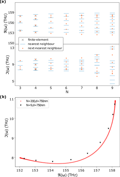
Figure 3: Comparison between numerical simulations and analytical model for $d=750~{}$nm. (a) Real part (top panel) and imaginary part (bottom panel) of the eigenfrequencies $\omega$ vs. the number N of resonators in the chain. Blue dashes: spectra calculated with the Hamiltonian model; grey crosses: FEM simulations. (b) Complex-plane representation of the analytically calculated eigenfrequencies for chains of $N=9$ (black triangles) and $N=200$ (red crosses).

IV Conclusion

Overall, the analytical non-Hermitian quantum formalism used here offers adequate means to compute modal information on 1D chains of $N$ resonators, and it can be naturally extended to nonlinear quantum optics [32]. By increasing the length of the chain, one could study the transition between a discrete ensemble of nanoresonators and a photonic crystal. Considering the wide variety of geometries and properties accessible via nanostructured dielectric materials, we envisage that such nanophotonic systems could be a promising model for implementing more complex interactions in 1D, 2D or 3D metasystems. They could also constitute toy systems to study for example topological edge states [33, 34]. A direct application for such a predictive model could be the improvement of Q factor optimization of leaky nanoresonators through non-Hermitian coupling.