From carriers and virtual excitons to exciton populations: Insights into time-resolved ARPES spectra from an exactly solvable model

Abstract

We calculate the exact time-resolved ARPES spectrum of a two-band model semiconductor driven out of equilibrium by resonant and nonresonant laser pulses, highlighting the effects of phonon-induced decoherence and relaxation. Resonant excitations initially yield a replica of the valence band shifted upward by the energy of the exciton peak in photoabsorption. This phase is eventually destroyed by phonon-induced decoherence: the valence-band replica lowers in energy by the Stokes shift, locating at the energy of the exciton peak in photoluminescence, and its width grows due to phonon dressing. Nonresonant excitations initially yield a map of the conduction band. Then electrons transfer their excess energy to the lattice and bind with the holes left behind to form excitons. In this relaxed regime a replica of the conduction band appears inside the gap. At fixed momentum the lineshape of the conduction-band replica versus the photoelectron energy is proportional to the exciton wavefunction in “energy space” and it is highly asymmetric. Although the two-band model represents an oversimplified description of real materials the highlighted features are qualitative in nature; hence they provide useful insights into time-resolved ARPES spectra and their physical interpretation.

I Introduction

Time-resolved and angle-resolved photoemission spectroscopy (trARPES) is currently one of the most flourishing playground for condensed matter theoreticians. Accurate approximations to the fundamental equations of many-body theory are being incessantly developed to relate the intensity and direction of the photocurrent to the behavior of quantum matter in equilibrium as well as nonequilibrium conditions. The relationship between pseudogap, charge ordering and Fermi arcs in high temperature superconductors Damascelli et al. (2003); Vishik (2018), Auger scattering, electron-phonon coupling, plasmonic excitations, and local screening in core excited metals Doniach and Sunjic (1970); Citrin et al. (1977); Hüfner (2003), carrier populations and conduction states in excited semiconductors Rossnagel (2012); Sangalli, D. and Marini, A. (2015); Smallwood et al. (2016); Mo (2017); Caruso et al. (2020), topological order Lv et al. (2019), excitonic insulator phases Wakisaka et al. (2009); Seki et al. (2014), excitonic Mott transitions Dendzik et al. (2020) and exciton dynamics Weinelt et al. (2004); Suzuki and Shimano (2009); Zhu (2015); Varene et al. (2012); Deinert et al. (2014); Perfetto et al. (2016); Steinhoff et al. (2017); Rustagi and Kemper (2018); Perfetto et al. (2019); Christiansen et al. (2019) in pumped semiconductors is a non exhaustive list of the plethora of different phenomena leaving distinctive footprints in trARPES spectra.

The interest in the exciton dynamics of (low-dimensional) semiconductors is steadily gaining momentum, especially due to potentially revolutionary applications in optoelectronics Jun et al. (2017). However, the physical interpretation of trARPES spectra is still subject of debates. The main difficulty in developing accurate many-body schemes suitable for numerical implementations lies in the treatment of electron-electron and electron-phonon scatterings under nonequilibrium conditions. We find useful to distinguish between two different nonequilibrium regimes: the linear-response regime, where the photocurrent is proportional to the intensity of the pump field, and the nonlinear regime. Making predictions in the nonlinear regime is certainly more difficult. Calculations are often limited to the quasi-equilibrium state of matter, a condition which allows for introducing more or less controlled approximations like, e.g., the invariance under time translations and the fulfillment of the fluctuation-dissipation theorem in different bands. The linear regime offers a wider set of theoretical tools; exciton formation, coherence and relaxation can be addressed in a more rigorous framework.

The trARPES signatures of excitons in linearly excited semiconductors is the topic of this work. In fact, there still are a few open questions pertaining with two distinct types of excitations. Resonant excitations are those of pump pulses with the same frequency as the energy $E^{(\rm x)}$ of a bright exciton. To avoid possible misinterpretations, by $E^{(\rm x)}$ we here denote the energy position of the excitonic peak in the photoabsorption spectrum of the ground-state system. Just after pumping a low-density gas of coherent excitons, also called nonequilibrium excitonic insulator or BEC exciton superfluid, forms Östreich and Schönhammer (1993); Hannewald et al. (2000a); Szymańska et al. (2006); Hanai et al. (2016, 2017); Becker et al. (2019). Theoretical works Kremp et al. (2008); Perfetto et al. (2016); Rustagi and Kemper (2018); Perfetto et al. (2019, 2020) predict an excitonic sideband in the ARPES spectrum – more precisely a replica of the valence band shifted upward by $E^{(\rm x)}$. The subsequent dynamics of the coherent exciton gas involves electron-phonon scatterings Hanai et al. (2016); Hannewald et al. (2000b), generation of phonons and phonon-induced decoherence Murakami et al. (2020), until the formation of a gas of incoherent excitons dressed by phonons, i.e., exciton-polarons. This incoherent phase is expected to set in on a time scale of a few hundreds of femtoseconds Sundaram and Mazur (2002); Bányai et al. (1995); Bar-Ad and Chemla (1997); Sangalli and Marini (2015) and it lasts until excitons radiatively recombine Palummo et al. (2015); Wang et al. (2018). To the best of our knowledge no theoretical ARPES studies exist in this phase. Is the excitonic sideband still visible? If so, is it any different from that of the coherent phase? Does the conduction band appear? Does the phonon bath relax? Besides strengthening our understanding an answer to these questions is becoming urgent. Recent experiments have indeed reported excitonic sidebands in a resonantly pumped WSe₂ monolayer after 0.5 picoseconds Man et al. (2020) and in a WSe₂ bulk until 0.1 picoseconds Dong et al. (2020).

The second type of excitation is generated by nonresonant pumping. Here the pump frequency is larger than the gap and electrons are promoted to empty conduction states. Just after pumping the ARPES spectrum provides a map of the conduction bands, the signal intensity being proportional to the band-resolved and momentum-resolved carrier populations. The excited electrons soon transfer their energy to the lattice, migrate toward the bottom of the conduction band Sangalli, D. and Marini, A. (2015); Caruso et al. (2020) and eventually bind with the left behind hole to form excitons Weinelt et al. (2004); Deinert et al. (2014). The spectral function in this relaxed (and incoherent) phase has been studied theoretically using the T-matrix approximation in the particle-hole channel assuming a quasi-thermal equilibrium Toyozawa (1986); Schepe et al. (1998); Piermarocchi and Tassone (2001); Kremp et al. (2008); Kwong et al. (2009); Asano and Yoshioka (2014); Perfetto et al. (2016); Steinhoff et al. (2017). The theory predicts an excitonic sideband inside the gap, about $E^{(\rm x)}$ above the valence band maximum. However, this spectral structure turns out to be a replica of the conduction band Asano and Yoshioka (2014); Perfetto et al. (2016); Steinhoff et al. (2017). Could this be the ultimate fate of the excitonic sideband for resonant excitations? May different excitations (resonant versus nonresonant) yield different sidebands (valence replica versus conduction replica) in the relaxed and incoherent phase? Couldn’t the replica of the conduction band be an artifact of the T-matrix approximation in combination with the assumption of quasi-thermal equilibrium?

We address the above issues through the exact analytic solution of a two-band model semiconductor where both electron-electron and electron-phonon interactions are taken into account. As the answer to the asked questions is qualitative in nature, our results provide a useful reference for benchmarking approximate many-body treatments. The main findings of our investigation are: (i) Incoherent excitons forming after resonant pumping do only change slightly the replica of the valence band (observed in the coherent phase); in particular the replica lowers in energy by the Stokes shift Toyozawa (2003) and its width grows due to phonon dressing (exciton-polarons); (ii) Phonon dressing is much faster than decoherence, the former being dictated by the largest phonon frequency whereas the latter by the smallest polaronic shift; (iii) Excitons forming after nonresonant pumping give rise to a replica of the conduction band, thus confirming the results of previous studies Asano and Yoshioka (2014); Perfetto et al. (2016); Steinhoff et al. (2017); for any fixed momentum the lineshape of the replica is determined by the exciton wavefunction in “energy space” and it is highly asymmetric.

The plan of the paper is as follows. In Section II we introduce the model and set up the problem; we also discuss the behavior of relevant observable quantities in different scenarios. The exact solution of the model for both acoustic and optical phonons is derived in Section III. We defer the reader to the Appendices for the calculation of the spectral function, momentum-resolved electron occupations, polarization and phonon occupations using the exact many-body wavefunction. Results for resonant and nonresonant excitations are presented in Sections  IV and V respectively. A summary of the main findings is drawn in Section VI.

II Exciton-polaron model

In standard notation the two-band model Hamiltonian reads

$$\hat{H} =\sum_{k}\big{(}\epsilon^{c}_{k}\hat{c}^{{\dagger}}_{k}\hat{c}_{k}+\epsilon^{v}_{k}\hat{v}^{{\dagger}}_{k}\hat{v}_{k}\big{)}+\sum_{q}\omega_{q}\hat{b}^{{\dagger}}_{q}\hat{b}_{q}$$

$$-\frac{1}{\mbox{$\mathcal{N}$}}\sum_{pk_{1}k_{2}}U_{p}\hat{c}^{{\dagger}}_{k_{1}+p}\hat{v}_{k_{2}+p}\hat{v}^{{\dagger}}_{k_{2}}\hat{c}_{k_{1}}$$

$$+\frac{1}{\sqrt{\mbox{$\mathcal{N}$}}}\sum_{kq}\lambda_{q}^{k}\big{(}\hat{c}^{{\dagger}}_{k+q}\hat{c}_{k}\hat{b}_{q}+\hat{c}^{{\dagger}}_{k}\hat{c}_{k+q}\hat{b}^{{\dagger}}_{q}\big{)}.$$ (1)

The first two terms describe free electrons in the valence ($v$) or conduction ($c$) band and free phonons. The remaining terms account for the electron-hole ($eh$) Coulomb interaction and the electron-phonon interaction; $\mathcal{N}$ is the number of discretized momenta in the first Brillouin zone. In our model only conduction electrons interact with phonons. However, the idea presented below can easily be adapted to include an interaction with valence electrons. The Hamiltonian in Eq. (1) has been studied numerically with Quantum Monte Carlo methods to address the dependence of the exciton-polaron wavefunction on the electron-phonon coupling Hohenadler et al. (2007); Burovski et al. (2008). We are not aware of other exact numerical or analytical treatments.

The state $|\Phi_{0}\rangle$ with a filled valence band, an empty conduction band and no phonons is an eigenstate of $\hat{H}$. We assume that the interaction $U_{p}$ is much larger than the energy gap $E_{g}$ between the conduction and valence bands. Then $|\Phi_{0}\rangle$ is the ground state and, without any loss of generality, we set to zero its energy. We now consider an ultrafast and low-intensity laser pulse pumping electrons from the valence band to the conduction band. To lowest order in the light intensity the state of the system at the end of the pulse can be written as

$$|\Psi\rangle=\alpha|\Phi_{0}\rangle+\beta|\Phi_{\rm x}\rangle,$$ (2)

with $\beta=\sqrt{1-\alpha^{2}}\ll 1$ and

$$|\Phi_{\rm x}\rangle=\sum_{k}Y^{0}_{k}\hat{c}^{{\dagger}}_{k}\hat{v}_{k}|\Phi_{0}\rangle$$ (3)

the component of the full many-body state with one electron in the conduction band, one hole in the valence band and no phonons. The coefficients $Y^{0}_{k}$ depend on the laser pulse parameters, e.g., duration and frequency. The state in Eq. (2) is not, in general, an eigenstate of $\hat{H}$. The pumped electron feels the attractive interaction with the hole left behind and it is scattered by phonons. We shall investigate two different physical scenario.

In the so called resonant case electrons are pumped at the exciton frequency and the state $|\Phi_{\rm x}\rangle$ is a bright excitonic eigenstate of the electronic part of $\hat{H}$. Discarding the electron-phonon interaction and denoting by $E^{(\rm x)}<E_{g}$ the exciton energy the evolution of the state $|\Psi\rangle$ would simply be

$$|\Psi(t)\rangle=\alpha|\Phi_{0}\rangle+\beta e^{-iE^{(\rm x)}t}|\Phi_{\rm x}\rangle.$$ (4)

As $|\Psi(t)\rangle$ has no phonons the electronic density matrix is a pure state

$$\hat{\rho}_{\rm el}(t)\equiv{\rm Tr}_{\rm ph}\big{\{}\,|\Psi(t)\rangle\langle\Psi(t)|\,\big{\}}=|\Psi(t)\rangle\langle\Psi(t)|,$$ (5)

where ${\rm Tr}_{\rm ph}$ signifies a trace over the phononic degrees of freedom. A system described by Eq. (5) is said to contain virtual or coherent excitons Haug et al. (1994); Schäfer and Wegener (2002). In fact, it is characterized by coherent oscillations of the polarization since the quantity

$${\rm Tr}_{\rm el}\left[\hat{\rho}_{\rm el}(t)\hat{v}^{{\dagger}}_{k}\hat{c}_{k}\right]=\alpha^{\ast}\beta\,Y^{0}_{k}e^{-iE^{(\rm x)}t}$$ (6)

oscillates at the exciton frequency for all $k$’s, see also Eq. (16) below. In Ref. Perfetto et al. (2020) we argued that these coherent oscillations could be observed in trARPES using ultrafast probes of duration shorter than $2\pi/E^{(\rm x)}$.

The state in Eq. (4) approximates the true time-dependent state only in the early stage of the evolution. Just after pumping electrons and phonons begin to scatter, mutually dressing each others, and the initial coherence is eventually destroyed. The electronic system is expected to evolve toward an admixture of $|\Phi_{0}\rangle$ and some exciton-like states $|\Phi^{(i)}_{\rm x}\rangle$:

$$\hat{\rho}_{\rm el}(t\to\infty) =\lim_{t\to\infty}{\rm Tr}_{\rm ph}\big{\{}\,|\Psi(t)\rangle\langle\Psi(t)|\,\big{\}}$$

$$=|\alpha|^{2}\,|\Phi_{0}\rangle\langle\Phi_{0}|+|\beta|^{2}\,\sum_{i}w_{i}|\Phi^{(i)}_{\rm x}\rangle\langle\Phi^{(i)}_{\rm x}|.$$ (7)

In this steady-state regime excitons are said real or incoherent and one can introduce the concept of exciton populations since the polarization does no longer oscillate. However, the existence and the characterization of the steady-state regime has so far been based on reasonable assumptions and it is still subject of debate. The purpose of this work is to provide useful insights into this issue through the exact solution of the time-dependent Schrödinger equation.

In the second scenario the laser pulse generates free carriers in the conduction band (nonresonant pumping). It is then expected that carriers give their excess energy to the lattice, thereby migrating toward the bottom of the conduction band and eventually binding with the holes left behind to form excitons. The phonon-driven formation of excitons is another debated topic in the literature as no real-time calculations are available to confirm this picture. Due to the simplicity of the model we could only address the dynamics of free carriers initially at the bottom of the conduction band.

Independently of the scenario we need to calculate the time-evolved state

$$|\Psi(t)\rangle \equiv e^{-i\hat{H}t}|\Psi\rangle=\alpha|\Phi_{0}\rangle+\beta|\Phi_{\rm x}(t)\rangle,$$ (8)

with

$$|\Phi_{\rm x}(t)\rangle=e^{-i\hat{H}t}\sum_{k}Y^{0}_{k}\hat{c}^{{\dagger}}_{k}\hat{v}_{k}|\Phi_{0}\rangle.$$ (9)

Henceforth we refer to $|\Phi_{\rm x}(t)\rangle$ as the exciton-polaron state although it may also describe unbound $eh$ pairs dressed by phonons. From $|\Phi_{\rm x}(t)\rangle$ we can monitor the momentum-resolved phonon occupations

$$n_{q}(t)=\langle\Phi_{\rm x}(t)|\hat{b}^{{\dagger}}_{q}\hat{b}_{q}|\Phi_{\rm x}(t)\rangle,$$ (10)

as well as the standard deviation of the phonon momentum

$$\sigma^{2}_{Q}(t) =\langle\Phi_{\rm x}(t)|\hat{Q}^{2}|\Phi_{\rm x}(t)\rangle-Q^{2}(t),$$ (11)

where $\hat{Q}=\sum_{q}q\,\hat{n}_{q}$ and $Q(t)=\sum_{q}q\,n_{q}$. We can also calculate the Green’s functions

$$G^{cc}_{k}(t,t^{\prime}) =i\langle\Psi(t^{\prime})|\hat{c}^{{\dagger}}_{k}e^{-i\hat{H}(t^{\prime}-t)}\hat{c}_{k}|\Psi(t)\rangle$$

$$=i|\beta|^{2}\langle\Phi_{\rm x}(t^{\prime})|\hat{c}^{{\dagger}}_{k}e^{-i\hat{H}(t^{\prime}-t)}\hat{c}_{k}|\Phi_{\rm x}(t)\rangle$$ (12)

and

$$G^{cv}_{k}(t,t^{\prime}) =i\langle\Psi(t^{\prime})|\hat{v}^{{\dagger}}_{k}e^{-i\hat{H}(t^{\prime}-t)}\hat{c}_{k}|\Psi(t)\rangle,$$

$$=i\alpha^{\ast}\beta e^{iE_{0}t^{\prime}}\langle\Phi_{0}|\hat{v}^{{\dagger}}_{k}e^{-i\hat{H}(t^{\prime}-t)}\hat{c}_{k}|\Phi_{\rm x}(t)\rangle.$$ (13)

The Green’s functions in Eqs. (12) and (13) contain information on the electronic transient spectrum, occupations and polarization. In fact, the ARPES signal of the system at time $T$ is proportional to the transient spectral function $A_{k}(T,\omega)$ which is in turn related to the Green’s function in Eq. (12) through (for $\omega$ above the valence band maximum)

$$A_{k}(T,\omega)=-i\int d\tau e^{i\omega\tau}G^{cc}_{k}(T+\frac{\tau}{2},T-\frac{\tau}{2}).$$ (14)

The electron occupations in the conduction band can also be obtained from the same Green’s function since

$$n^{c}_{k}(t)=\langle\Psi(t)|\hat{c}_{k}^{{\dagger}}\hat{c}_{k}|\Psi(t)\rangle=-iG^{cc}_{k}(t,t).$$ (15)

Denoting by $d_{k}$ the dipole matrix element between a conduction state and a valence state of momentum $k$ the polarization at time $t$ reads

$$P(t) =\frac{1}{\mbox{$\mathcal{N}$}}\sum_{k}d_{k}\langle\Psi(t)|\hat{v}^{{\dagger}}_{k}\hat{c}_{k}|\Psi(t)\rangle+{\rm h.c.}$$

$$=-\frac{i}{\mbox{$\mathcal{N}$}}\sum_{k}d_{k}G^{cv}_{k}(t,t)+{\rm h.c.}\;.$$ (16)

In the next section we expand the exciton-polaron state on a convenient basis and calculate the time-dependent expansion coefficients.

III Time-dependent exciton-polaron wave-function

We introduce the states

$$|kq_{1}\ldots q_{M}\rangle=\hat{c}^{{\dagger}}_{k-q_{1}\ldots-q_{M}}\hat{v}_{k}\hat{b}^{{\dagger}}_{q_{1}}\ldots\hat{b}^{{\dagger}}_{q_{M}}|\Phi_{0}\rangle,$$ (17)

describing one $eh$ pair and $M$ phonons. In terms of these states Eq. (3) can be written as $|\Phi_{\rm x}\rangle=\sum_{k}Y^{0}_{k}|k\rangle$. Hence the calculation of $|\Phi_{\rm x}(t)\rangle$ passes through the calculation of $e^{-i\hat{H}t}|k\rangle$. The Hamiltonian $\hat{H}$ maps the space spanned by the states of Eq. (17) onto the same space since

$$\hat{H}|kq_{1}\ldots q_{M}\rangle =\big{(}\epsilon^{c}_{k-q_{1}\ldots-q_{M}}-\epsilon^{v}_{k}+\sum_{j=1}^{M}\omega_{q_{j}}\big{)}|kq_{1}\ldots q_{M}\rangle$$

$$-\frac{1}{\mbox{$\mathcal{N}$}}\sum_{p}U_{p}|k+pq_{1}\ldots q_{M}\rangle$$

$$+\frac{1}{\sqrt{\mbox{$\mathcal{N}$}}}\sum_{j=1}^{M}\lambda^{k}_{q_{j}}|kq_{1}\ldots\stackrel{{\scriptstyle\sqcap}}{{q}}_{j}\ldots q_{M}\rangle$$

$$+\frac{1}{\sqrt{\mbox{$\mathcal{N}$}}}\sum_{q}\lambda^{k}_{q}|kqq_{1}\ldots q_{M}\rangle,$$ (18)

where the square-cap symbol “$\stackrel{{\scriptstyle\sqcap}}{{}}$” signifies that the index below it is missing. We can therefore expand the exciton-polaron state as

$$|\Phi_{\rm x}(t)\rangle=\sum_{M=0}^{\infty}\frac{1}{M!}\sum_{k,q_{1}\ldots q_{M}}Y_{kq_{1}\ldots q_{M}}(t)|kq_{1}\ldots q_{M}\rangle.$$ (19)

Without any loss of generality we take the amplitudes $Y_{kq_{1}\ldots q_{M}}$ totally symmetric under a permutation of the phonon indices $\{q_{1},\ldots,q_{M}\}$ – only this irreducible representation contributes in the sum of Eq. (19). Using the inner product,

$$\langle k^{\prime}q_{1}^{\prime}\ldots q^{\prime}_{M}|kq_{1}\ldots q_{M}\rangle=\delta_{k^{\prime}k}\sum_{P}\prod_{j=1}^{M}\delta_{q^{\prime}_{j}q_{P(j)}},$$ (20)

where the sum runs over all permutations of $\{1,\ldots,M\}$, we find

$$\langle kq_{1}\ldots q_{M}|e^{-i\hat{H}t}|\Phi_{\rm x}\rangle=Y_{kq_{1}\ldots q_{M}}(t).$$ (21)

Equations (18) and (21) allows for generating a hierarchy of differential equations for the amplitudes

$$i\dot{Y}_{kq_{1}\ldots q_{M}}(t) =\langle kq_{1}\ldots q_{M}|\hat{H}e^{-i\hat{H}t}|\Phi_{\rm x}\rangle$$

$$=\big{(}\epsilon^{c}_{k-q_{1}\ldots-q_{M}}-\epsilon^{v}_{k}+\sum_{j=1}^{M}\omega_{q_{j}}\big{)}Y_{kq_{1}\ldots q_{M}}(t)$$

$$-\frac{1}{\mbox{$\mathcal{N}$}}\sum_{p}U_{p}Y_{k+pq_{1}\ldots q_{M}}(t)$$

$$+\frac{1}{\sqrt{\mbox{$\mathcal{N}$}}}\sum_{j=1}^{M}\lambda^{k}_{q_{j}}Y_{kq_{1}\ldots\stackrel{{\scriptstyle\sqcap}}{{q}}_{j}\ldots q_{M}}(t)$$

$$+\frac{1}{\sqrt{\mbox{$\mathcal{N}$}}}\sum_{q}\lambda^{k}_{q}Y_{kqq_{1}\ldots q_{M}}(t).$$ (22)

Already at this stage we can discuss the conditions for the development of an incoherent regime. Taking into account Eqs. (8) and (19) we find for the electronic density matrix

$$\hat{\rho}_{\rm el}(t) =|\alpha|^{2}|\Phi_{0}\rangle\langle\Phi_{0}|$$

$$+|\beta|^{2}\sum_{M=0}^{\infty}\frac{1}{M!}\sum_{q_{1}\ldots q_{M}}|\Phi_{{\rm x},q_{1}\ldots q_{M}}(t)\rangle\langle\Phi_{{\rm x},q_{1}\ldots q_{M}}(t)|$$

$$+\left(\beta\alpha^{\ast}\sum_{k}Y_{k}(t)|k\rangle\langle\Phi_{0}|+{\rm h.c.}\right),$$ (23)

where we have defined

$$|\Phi_{{\rm x},q_{1}\ldots q_{M}}(t)\rangle\equiv\sum_{k}Y_{kq_{1}\ldots q_{M}}(t)|k\rangle.$$ (24)

A direct comparison with Eq. (7) shows that for the system to relax toward an incoherent steady-state the zero-phonon amplitude $Y_{k}(t)$ must vanish as $t\to\infty$ and

$$\lim_{t\to\infty}\sum_{M=0}^{\infty}\frac{1}{M!}\sum_{q_{1}\ldots q_{M}}Y_{kq_{1}\ldots q_{M}}(t)Y^{\ast}_{k^{\prime}q_{1}\ldots q_{M}}(t)=\sum_{i}w_{i}\mbox{$\mathcal{Y}$}^{i}_{k}\mbox{$\mathcal{Y}$}^{i\ast}_{k^{\prime}},$$ (25)

where $\mbox{$\mathcal{Y}$}_{k}^{i}$ are some $k$-dependent and time-independent complex quantities. We shall comment on the fulfillment of these properties using the exact solution.

The hierarchy in Eq. (22) can be solved analytically in some special, yet relevant, cases. The first condition to meet is

$$\epsilon^{c}_{k-q_{1}\ldots-q_{M}}=\epsilon^{c}_{k}$$ (26)

for all $\{q_{1},\ldots,q_{M}\}$ and for all $M$. Rigorously this condition is satisfied only for a perfectly flat conduction band. However, Eq. (26) is a good approximation for couplings $\lambda$’s and frequencies $\omega$’s such that the distribution of phonon-momenta has a peak around $q=0$ with standard deviation $\sigma_{Q}$ much smaller than the momentum-scale over which the dispersion $\epsilon^{c}_{k}$ varies. No restrictions on the dispersion of the valence band $\epsilon^{v}_{k}$ are imposed.

Let us introduce the vectors

$$({\mathbf{Y}}_{q_{1}\ldots q_{M}})_{k}=Y_{kq_{1}\ldots q_{M}}$$ (27)

and the matrices

$$\mathbb{H}_{kk^{\prime}}=\delta_{kk^{\prime}}(\epsilon^{c}_{k}-\epsilon^{v}_{k})-\frac{U_{p-k}}{\mbox{$\mathcal{N}$}}\quad;\quad\mathbb{L}_{q,kk^{\prime}}=\delta_{kk^{\prime}}\lambda^{k}_{q}.$$ (28)

Then the hierarchy in Eq. (22) can be rewritten in matrix form as (omitting the dependence on time)

$$i\dot{{\mathbf{Y}}}_{q_{1}\ldots q_{M}} =(\mathbb{H}+\omega_{q_{1}}\ldots+\omega_{q_{M}}){\mathbf{Y}}_{q_{1}\ldots q_{M}}$$

$$+\sum_{j=1}^{M}\frac{\mathbb{L}_{q_{j}}}{\sqrt{\mbox{$\mathcal{N}$}}}{\mathbf{Y}}_{q_{1}\ldots\stackrel{{\scriptstyle\sqcap}}{{q}}_{j}\ldots q_{M}}+\sum_{q}\frac{\mathbb{L}_{q}}{\sqrt{\mbox{$\mathcal{N}$}}}{\mathbf{Y}}_{qq_{1}\ldots q_{M}}.$$ (29)

Notice that the matrix $\mathbb{H}$ is the Bethe-Salpeter Hamiltonian for an $eh$ pair. Hence the spectrum of $\mathbb{H}$ consists of a discrete excitonic part with subgap eigenvalues and a continuum $eh$ part with eigenvalues larger than the gap.

III.1 $q$-independent coupling

We consider optical phonons $\omega_{q}=\omega_{0}$ and coupling matrices $\mathbb{L}_{q}=\mathbb{L}$ depending only on the electron momentum, hence $\lambda^{k}_{q}=\lambda^{k}$. In this case all coefficients of the hierarchy are independent of the phonon momenta. We look for solutions of the form

$${\mathbf{Y}}_{q_{1}\ldots q_{M}}(t)=\sqrt{\frac{M!}{\mbox{$\mathcal{N}$}^{M}}}{\mathbf{Y}}_{M}(t).$$ (30)

Inserting Eq. (30) into Eq. (29) we find a closed system of equations for the ${\mathbf{Y}}_{M}$’s

$$i\dot{{\mathbf{Y}}}_{M}=(\mathbb{H}+M\omega_{0}){\mathbf{Y}}_{M}+\sqrt{M}\mathbb{L}{\mathbf{Y}}_{M-1}+\sqrt{M+1}\mathbb{L}{\mathbf{Y}}_{M+1}.$$ (31)

This simplified hierarchy can easily be solved with continued matrix fraction techniques Martinez (2003); Stefanucci et al. (2008). The time evolved state in Eq. (19) then reads

$$|\Phi_{\rm x}(t)\rangle=\sum_{M=0}^{\infty}\sum_{k}\frac{Y_{kM}(t)}{\sqrt{M!}}|kM\rangle,$$ (32)

where

$$|kM\rangle\equiv\frac{1}{\sqrt{\mbox{$\mathcal{N}$}^{M}}}\sum_{q_{1}\ldots q_{M}}|kq_{1}\ldots q_{M}\rangle.$$ (33)

For arbitrary initial conditions ${\mathbf{Y}}_{M}(0)=\delta_{M0}{\mathbf{Y}}^{0}$ no steady state is ever attained in the long time limit. This means that the electronic density matrix does not evolve toward an admixture like in Eq. (7). Nonetheless, the spectral function $A_{k}(T,\omega)$ becomes independent of $T$ as $T\to\infty$ if the probing time, i.e., the $\tau$-window of integration in Eq. (14), is much longer than $2\pi/\omega_{0}$.

It is instructive to expand the vectors ${\mathbf{Y}}_{M}$ in eigenvectors ${\mathbf{Y}}^{(\mu)}$ with energies $E^{(\mu)}$ of the Bethe-Salpeter Hamiltonian $\mathbb{H}$

$${\mathbf{Y}}_{M}(t)=\sum_{\mu}\alpha_{\mu M}(t){\mathbf{Y}}^{(\mu)}.$$ (34)

The hierarchy in Eq. (31) can be used to obtain a hierarchy for the coefficients of the expansion

$$i\dot{\alpha}_{\mu M} =(E^{(\mu)}+M\omega_{0})\alpha_{\mu M}$$

$$+\sum_{\nu}L_{\mu\nu}\left[\sqrt{M}\alpha_{\nu M-1}+\sqrt{M+1}\alpha_{\nu M+1}\right],$$ (35)

where we have defined

$$L_{\mu\nu}\equiv{\mathbf{Y}}^{(\mu){\dagger}}\mathbb{L}{\mathbf{Y}}^{(\nu)}.$$ (36)

If the coupling $\lambda^{k}$ depends on $k$ then the matrix element $L_{\mu\nu}$ is, in general, nonvanishing for $\mu\neq\nu$. This implies that even if there are no phonons at time $t=0$ and the zero-phonon component $Y_{0}(0)=Y^{(\mu_{0})}$ is an eigenstate of $\mathbb{H}$, hence $\alpha_{\mu M}(0)=\delta_{0M}\delta_{\mu_{0}\mu}$, electronic states with $\nu\neq\mu_{0}$ are visited during the evolution.

III.2 $k$-independent coupling

The hierarchy in Eq. (29) can be solved exactly also in the special case $\mathbb{L}_{q}=\lambda_{q}\mathbb{1}$, i.e., for an electron-phonon coupling $\lambda^{k}_{q}=\lambda_{q}$ independent of the electronic momentum. No restrictions on the phonon frequencies is necessary in this case. We define

$${\mathbf{Y}}_{q_{1}\ldots q_{M}}(t)=e^{-i\mathbb{H}t}{\mathbf{X}}_{q_{1}\ldots q_{M}}(t),$$ (37)

and rewrite the hierarchy for the vectors ${\mathbf{X}}$’s

$$i\dot{{\mathbf{X}}}_{q_{1}\ldots q_{M}} =(\omega_{q_{1}}\ldots+\omega_{q_{M}}){\mathbf{X}}_{q_{1}\ldots q_{M}}$$

$$+\sum_{j=1}^{M}\frac{\lambda_{q_{j}}}{\sqrt{\mbox{$\mathcal{N}$}}}{\mathbf{X}}_{q_{1}\ldots\stackrel{{\scriptstyle\sqcap}}{{q}}_{j}\ldots q_{M}}+\sum_{q}\frac{\lambda_{q}}{\sqrt{\mbox{$\mathcal{N}$}}}{\mathbf{X}}_{qq_{1}\ldots q_{M}}.$$ (38)

We look for solutions of the form

$${\mathbf{X}}_{q_{1}\ldots q_{M}}(t)=f_{q_{1}}(t)\ldots f_{q_{M}}(t){\mathbf{X}}(t).$$ (39)

Inserting Eq. (39) into Eq. (38) we find that the hierarchy is solved provided that

$$i\dot{f}_{q}=\frac{\lambda_{q}}{\sqrt{\mbox{$\mathcal{N}$}}}+\omega_{q}f_{q},$$ (40)

and

$$i\dot{{\mathbf{X}}}=\sum_{q}\frac{\lambda_{q}}{\sqrt{\mbox{$\mathcal{N}$}}}f_{q}(t){\mathbf{X}}.$$ (41)

The solution of Eq. (40) with boundary condition $f_{q}(0)=0$ (no phonons at the initial time) is the Langreth function Langreth (1970)

$$f_{q}(t)=\frac{1}{\sqrt{\mbox{$\mathcal{N}$}}}\frac{\lambda_{q}}{\omega_{q}}(e^{-i\omega_{q}t}-1).$$ (42)

Substituting the explicit form of $f_{q}(t)$ into Eq. (41) we find

$${\mathbf{X}}(t)=\ell(t){\mathbf{X}}(0),$$ (43)

with

$$\ell(t)=\exp\left[\frac{1}{\mbox{$\mathcal{N}$}}\sum_{q}\left(\frac{\lambda_{q}}{\omega_{q}}\right)^{2}(-1+e^{-i\omega_{q}t}+i\omega_{q}t)\right].$$ (44)

Taking into account Eqs. (37) and (39) we eventually get

$${\mathbf{Y}}_{q_{1}\ldots q_{M}}(t)=f_{q_{1}}(t)\ldots f_{q_{M}}(t)\ell(t){\mathbf{Y}}^{0}(t),$$ (45)

where ${\mathbf{Y}}^{0}(t)=e^{-i\mathbb{H}t}{\mathbf{Y}}^{0}$ and $({\mathbf{Y}}^{0})_{k}=Y^{0}_{k}$ are the amplitudes of the state $|\Phi_{\rm x}\rangle$. In Eq. (45) the phonon dynamics is decoupled from the electron dynamics. If the initial state is an eigenstate of $\mathbb{H}$, i.e., ${\mathbf{Y}}^{0}={\mathbf{Y}}^{(\mu_{0})}$ then no other electronic state is visited at later times.

For acoustic phonons the function $\ell(t)$ vanishes as $t\to\infty$ and therefore $Y_{k}(t)=\ell(t)Y^{0}_{k}(t)$ vanishes too in the same limit. This implies that the electronic density matrix becomes an admixture in the long-time limit, see Eq. (23). To determine the nature of this admixture we have to evaluate Eq. (25). Taking into account that $|\ell(t)|^{2}=\exp[-\sum_{q}|f_{q}(t)|^{2}]$ it is straightforward to find

$$\lim_{t\to\infty}\hat{\rho}_{\rm el}(t)=|\alpha|^{2}|\Phi_{0}\rangle\langle\Phi_{0}|+|\beta|^{2}|\Phi_{\rm x}^{(0)}(t)\rangle\langle\Phi_{\rm x}^{(0)}(t)|$$ (46)

with $|\Phi_{\rm x}^{(0)}(t)\rangle=\sum_{k}Y^{0}_{k}(t)|k\rangle$. Therefore the admixture contains only two states and for it to attain a steady state the initially pumped state must be an eigenstate of the electron Hamiltonian $\mathbb{H}$. In particular if the initial state is the excitonic eigenstate then $Y^{0}_{k}(t)=e^{-iE^{(\rm x)}t}Y_{k}^{(\rm x)}$ and

$$\lim_{t\to\infty}\hat{\rho}_{\rm el}(t)=|\alpha|^{2}|\Phi_{0}\rangle\langle\Phi_{0}|+|\beta|^{2}|\Phi_{\rm x}\rangle\langle\Phi_{\rm x}|.$$ (47)

Comparing this result with the electronic density matrix at the initial time, see Eqs. (4) and (5), we conclude that the two-band model is able to describe the complete loss of coherence due to scattering of electrons with acoustic phonons.

IV Resonant pumping

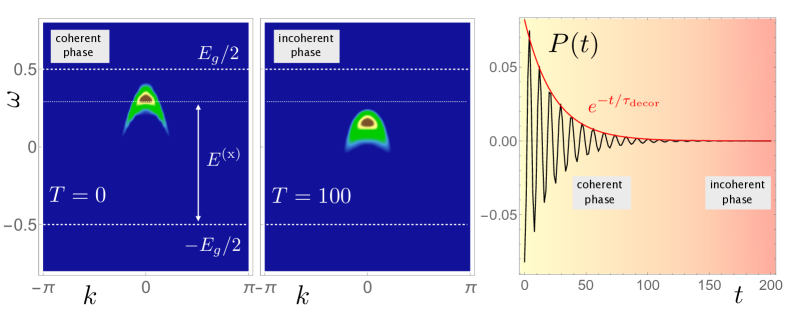
Figure 1: Spectral function of the interacting electron-phonon system for $T=0$ (left) and $T=100$ (middle). Tick-dashed lines have been drawn in correspondence of the CBM and VBM. Thin-dashed lines have been drawn in correspondence of the exciton energy. The right panel shows the time-dependent polarization calculated with $d_{k}=d$ for all $k$-points.

We investigate the effects of phonon dressing and decoherence in a semiconductor driven by coherent light of frequency in resonance with the energy of a bright exciton (resonant pumping). For illustration we consider a 1D model with a flat conduction band $\epsilon_{k}^{c}=\epsilon_{c}=E_{g}/2$ [conduction band minimum (CBM) at $E_{g}/2$] and a dispersive valence band $\epsilon^{v}_{k}=E_{g}[\cos k-1]-E_{g}/2$ [valence band maximum (VBM) at $-E_{g}/2$] separated by an energy gap $E_{g}$. Henceforth all energies are measured in units of $E_{g}$ and times in units of $1/E_{g}$. For a short-range (momentum-independent) Coulomb interaction $U_{p}=U=0.65$ the electronic system admits an exciton state ${\mathbf{Y}}^{(\rm x)}$ of energy $E^{(\rm x)}\simeq 0.81$. Under the condition of resonant pumping the initial state is therefore ${\mathbf{Y}}^{0}={\mathbf{Y}}^{(\rm x)}$.

Without electron-phonon scattering, i.e., $\lambda^{k}_{q}=0$, the spectral function $A_{k}(T,\omega)$ in Eq. (14) is independent of $T$ and for each $k$ it exhibits a single peak at energy $\epsilon^{v}_{k}+E^{(\rm x)}$ Kremp et al. (2008); Perfetto et al. (2016); Rustagi and Kemper (2018); Perfetto et al. (2019), see also Appendix A:

$$A_{k}(T,\omega)=2\pi|\beta|^{2}\left|Y^{(\rm x)}_{k}\right|^{2}\delta(\omega-\epsilon^{v}_{k}-E^{(\rm x)}).$$ (48)

This spectral function can be interpreted as the fully interacting spectral function just after the excitation, i.e., at $T=0$ – phonon scatterings kick in only at later times. Equation (48) yields an excitonic sideband; it is a replica of the valence band located at energy $E^{(\rm x)}$ above the VBM with spectral weight proportional to the square of the excitonic wavefunction. In Fig. 1 (left) we show the color plot of Eq. (14). Calculations have been performed with $\mbox{$\mathcal{N}$}=81$ $k$-points using a $\tau$-window of integration that extends from $\tau_{\rm min}=-60$ to $\tau_{\rm max}=-\tau_{\rm min}$.

The electron-phonon coupling causes the spectral function to acquire a dependence on $T$, even for initial states that are eigenstates of $\mathbb{H}$. We study the evolution of the system when conduction electrons interact through a coupling $\lambda_{q}=\frac{\lambda_{0}}{2}(\cos q+1)$ with acoustic phonons of dispersion $\omega_{q}=\omega_{s}\sin|q|$. In the numerical simulations we have chosen $\lambda_{0}=0.18$ and $\omega_{s}=2(E_{g}-E^{(\rm x)})=0.38$ – which is twice the exciton binding energy. In Appendix B we demonstrate that the polarization $P(t)$ in Eq. (16) can be written as

$$P(t)=\alpha^{\ast}\beta\frac{1}{\mbox{$\mathcal{N}$}}\sum_{k}d_{k}Y_{k}(t)+{\rm h.c.}$$ (49)

where $Y_{k}(t)=\ell(t)e^{-iE^{(\rm x)}t}Y^{0}_{k}$, see Eq. (45). Let us briefly discuss the behavior of $P(t)$ for a vanishing electron-phonon coupling. In this case $\ell(t)=1$ and the polarization oscillates monochromatically at frequency $E^{(\rm x)}$. In the diagrammatic nonequilibrium Green’s function theory a simple Hartree-Fock (HF) treatment of the Coulomb interaction is enough to reproduce the oscillatory behavior Schmitt-Rink et al. (1988); Östreich and Schönhammer (1993); Schäfer and Treusch (1986); Lindberg and Koch (1988); Perfetto et al. (2019). Interestingly, the HF theory also predicts the appearance of the excitonic sideband in the spectral function, see Eq. (48). The coherent oscillations of $P(t)$ are crucial to observe this effect, which does indeed originate from the eigenvalues of the HF Floquet Hamiltonian Perfetto and Stefanucci (2020). Switching on the electron-phonon coupling the function $\ell(t)$, and hence the amplitude $Y_{k}(t)$, vanishes for $t\to\infty$. In Fig. 1 (right) we show $P(t)$ for a system with dipole matrix elements $d_{k}=d$ for all $k$. For $t\simeq 100$ the polarization is suppressed by about two order of magnitudes. We shall show that in this incoherent phase (times $t>100$) the exact spectral function still exhibits an excitonic sideband. Therefore excitonic structures in the spectral function are not a hallmark of excitonic coherence, as it is erroneously predicted by the HF theory.

To obtain the spectral function in the incoherent regime we evaluated Eq. (14), see Appendix A, at $T=100$ using the same $\tau$-window of integration as in the left panel of Fig. 1. The result is shown in the middle panel of the same figure. The excitonic sideband is still clearly visible although it is slightly shifted downward. In fact, it would be more appropriate to refer to this spectral feature as the exciton-polaron sideband. The experiment of Ref. Man et al. (2020) has most likely measured such sideband as the system was probed after 0.5 picoseconds from the resonant excitation. We also observe that phonon-dressing is responsible for an energy broadening of the sideband, consistently with the reported damping of the polarization.

The energy shift of the excitonic sideband as the system evolves from the coherent to the incoherent phase can also be related to the Stokes shift Toyozawa (2003). At zero momentum the coherent peak is detected at energy $E^{(\rm x)}$, i.e., at the onset of the photoabsorption spectrum, whereas the incoherent peak is red shifted by the “reorganization energy”, i.e., the energy gain in the transition from an exciton to an exciton-polaron. Therefore the energy of the incoherent peak lies at the onset of the photoluminescence spectrum Li et al. (2019); Hoyer et al. (2005). This also agrees with the fact that the photoluminescence signal is proportional to the population of (incoherent) excitons Hannewald et al. (2000b). In this respect trARPES provides a unique investigation tool as it allows for extracting information which would otherwise require two independent experiments, i.e., absorption and luminescence.

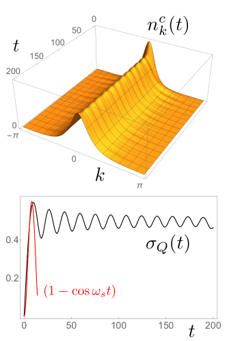
Figure 2: Top: Time-dependent $k$-resolved electronic occupations in the conduction band. Bottom: Time-dependent standard deviation of the phonon momentum.

In Fig. 2 (top) we show the evolution of the $k$-resolved electron density in the conduction band. At time $t=0$ the profile is proportional to the square of the exciton wavefunction in momentum space, i.e., $n^{c}_{k}(0)\propto|Y^{(\rm x)}_{k}|^{2}$, see Appendix A. As time increases the exciton transforms into an exciton-polaron and the wavefunction slightly spreads. Thus the dressed $eh$ wavepacket becomes more localized in real-space, in agreement with the larger binding energy observed in Fig. 1 (middle). We observe that the phonon dressing occurs on a much faster time-scale than the decoherence time, i.e., the timescale over which the polarization damps. This can also be seen from the plot of the time-dependent standard deviation $\sigma_{Q}(t)$, see Fig. 2 (bottom). According to Eq. (90) the standard deviation grows like $\sigma_{Q}(t)\propto(1-\cos\omega_{s}t)$. Hence the timescale $\tau_{\rm dress}$ for the phonon dressing is

$$\tau_{\rm dress}=\frac{2\pi}{\omega_{s}}\simeq 16.3.$$ (50)

The envelope function of the polarization can be found from Eq. (49). After some simple algebra one finds an approximate exponential decay $\exp[-t/\tau_{\rm decoh}]$ with decoherence time

$$\tau_{\rm decoh}=\frac{\omega_{s}}{2\lambda_{0}^{2}}=23.8.$$ (51)

In Fig. 1 (right) the envelope function nicely interpolates all maxima of the time-dependent polarization, see red curve. We emphasize that the dressing time is dictated by the largest phonon frequency whereas the decoherence time is dictated by the smallest polaronic shift. Furthermore, the dressing timescale does not appear in an exponential function, see again Fig. 2. We also notice that $\sigma_{Q}(t)\simeq 0.5$ in the long-time limit; hence, similar results would have been obtained for a dispersive conduction band with a shallow enough minimum.

Although the electronic occupations as well as the polarization attain a steady value in the long time limit the phononic occupations do not. This behavior is a direct consequence of the acoustic dispersion and the low dimensionality. In Appendix C we demonstrate that $n_{q}(t)=|f_{q}(t)|^{2}$ where the function $f_{q}(t)$ is given in Eq. (42). Therefore the total number of phonons at time $t$ is given by $N_{\rm ph}(t)=\frac{2}{\mbox{$\mathcal{N}$}}\sum_{q}(\frac{\lambda_{q}}{\omega_{q}})^{2}(1-\cos\omega_{q}t)$. For large times the main contribution to the sum comes from low-momentum phonons. Approximating $\omega_{q}\simeq\omega_{s}|q|$, $\lambda_{q}\simeq\lambda_{0}$ and taking the thermodynamic limit $\mbox{$\mathcal{N}$}\to\infty$ we then find

$$N_{\rm ph}(t)\simeq\frac{\lambda_{0}^{2}}{\omega_{s}}\,t=\frac{1}{2}\frac{t}{\tau_{\rm decoh}}.$$ (52)

Thus the total number of phonons increases linearly in time. It is easy to show that the divergence of $N_{\rm ph}(t)$ at $t\to\infty$ is milder in two dimensions, being it $\log(t)$, and it is absent in three dimensions. We also observe that the free-phonon contribution to the total energy $E_{\rm ph}(t)=\sum_{q}\omega_{q}n_{q}(t)$ diverges like $\log(t)$ in one dimension whereas it approaches a constant value for larger dimensions.

V Nonresonant pumping

Electrons pumped in the conduction band have enough energy to emit optical phonons and hence to decay into a bound exciton state. The issue we intend to address here is whether the spectral function exhibits an excitonic structure inside the gap and, in the affirmative case, what the shape is.

As already pointed out the exact solution of the two-band model Hamiltonian does not attain a steady state for optical phonons, see discussion in Section III.1. However, probing the system with pulses of duration much longer than the inverse of the phonon frequency the spectral function $A_{k}(T,\omega)$ becomes independent of $T$ as $T\to\infty$. We consider again a 1D model with a flat conduction band and a dispersive valence band separated by an energy gap $E_{g}$: $\epsilon_{k}^{c}=\epsilon_{c}=E_{g}/2$ (CBM at $E_{g}/2$) and $\epsilon^{v}_{k}=E_{g}[\cos k-1]-E_{g}/2$ (VBM at $-E_{g}/2$). We also consider the same short-range Coulomb interaction $U_{p}=0.65$ (all energies are in units of $E_{g}$) as in the previous section – hence the system admits one exciton state at energy $E^{(\rm x)}=0.31$. Let us assume that the pump has excited the system in a wavepacket of continuum $eh$ states ${\mathbf{Y}}^{(c)}$ of the Bethe-Salpeter Hamiltonian $\mathbb{H}$ with energy $E^{(c)}\simeq E_{g}$, hence

$${\mathbf{Y}}^{0}=\frac{1}{\sqrt{\mbox{$\mathcal{N}$}_{0}}}\sum_{c:E^{(c)}\simeq E_{g}}{\mathbf{Y}}^{(c)},$$ (53)

where $\mbox{$\mathcal{N}$}_{0}$ is the number of eigenstates in the sum. In the thermodynamic limit the ratio $r_{0}=\mbox{$\mathcal{N}$}_{0}/\mbox{$\mathcal{N}$}\ll 1$ remains finite. At zero pump-probe delay, i.e., $T=0$, we can ignore phonon effects and the spectral function reads [compare with the resonant case Eq. (48)]:

$$A_{k}(0,\omega)=2\pi|\beta|^{2}\Big{|}Y^{0}_{k}\Big{|}^{2}\delta(\omega-E_{g}/2).$$ (54)

As $Y^{0}_{k}$ is peaked around $k=0$ the spectral function $A_{k\simeq 0}(0,\omega)$ is peaked at frequency $\omega\simeq E_{g}/2=\epsilon^{c}$ (CBM), and it is vanishingly small for nonvanishing momenta.

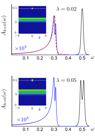
Figure 3: Spectral function $A_{k\simeq 0}(\omega)$ in the long-time limit $T\to\infty$ for a weak ($\lambda_{0}=0.02$, top panel) and intermediate ($\lambda_{0}=0.05$, bottom panel) electron-phonon coupling. The exciton contribution (blue line) is magnified by a factor $10^{4}$ (top) and $10^{3}$ (bottom). The dashed (red) line in the top panel is the exciton wavefunction in energy space, see main text. The insets show the color plot of the spectral function in the $k-\omega$ plane.

In Appendix A we show that for electrons coupled to a branch of optical phonons of frequency $\omega_{0}$ the spectral function in the long-time limit becomes

$$\lim_{T\to\infty}A_{k}(T,\omega) =\lim_{T\to\infty}\frac{|\beta|^{2}}{T}\times\Big{\{}\Big{|}\tilde{Y}_{k0}(\omega-\epsilon^{v}_{k})\Big{|}^{2}$$

$$+\sum_{M=1}^{\infty}\frac{1}{\mbox{$\mathcal{N}$}}\sum_{p}\Big{|}\tilde{Y}_{pM}(\omega-\epsilon^{v}_{p}+M\omega_{0})\Big{|}^{2}\Big{\}}.$$ (55)

The amplitudes $\tilde{{\mathbf{Y}}}_{M}(\omega)$ are the Fourier transform of the time-dependent amplitudes ${\mathbf{Y}}_{M}(t)$ in Eq. (31). Interestingly only the first term ($M=0$) depends on $k$. All remaining terms ($M\geq 1$) contribute with a $k$-independent function of the frequency (a consequence of the nondispersive nature of the conduction band). Expanding the amplitudes like in Eq. (34) we can equivalently calculate $\tilde{{\mathbf{Y}}}_{M}(\omega)$ from the Fourier transform of the hierarchy in Eq. (35). We neglect here the couplings $L_{cc^{\prime}}$ between low-energy continuum states since these scatterings are suppressed by energy conservation. We instead consider the couplings $L_{c\rm x}=L_{{\rm x}c}=\lambda_{0}/\sqrt{\mbox{$\mathcal{N}$}}$ between the exciton state and the continuum states. We then find

$$i\dot{\alpha}_{cM} =(E^{(c)}+M\omega_{0})\alpha_{cM}$$

$$+\frac{\lambda_{0}}{\sqrt{\mbox{$\mathcal{N}$}}}\left[\sqrt{M}\alpha_{{\rm x}M-1}+\sqrt{M+1}\alpha_{{\rm x}M+1}\right],$$ (56)

$$i\dot{\alpha}_{{\rm x}M} =(E^{(\rm x)}+M\omega_{0})\alpha_{{\rm x}M}$$

$$+\frac{\lambda_{0}}{\sqrt{\mbox{$\mathcal{N}$}}}\sum_{c}\left[\sqrt{M}\alpha_{cM-1}+\sqrt{M+1}\alpha_{cM+1}\right],$$ (57)

to be solved with boundary conditions $\alpha_{cM}(0)=\delta_{M0}/\sqrt{\mbox{$\mathcal{N}$}_{0}}$ if $E^{(c)}\simeq E_{g}$ and zero otherwise, see Eq. (53). The symmetry of the electron-phonon coupling preserves the symmetry of the initial state, i.e., $\alpha_{cM}(t)$ is independent of $c$ if $E^{(c)}\simeq E_{g}$ and $\alpha_{cM}(t)=0$ otherwise. We can therefore simplify the hierarchy by introducing the quantity $\alpha_{0M}(t)=\sum_{c}\alpha_{cM}(t)$ and by taking into account that $E^{(c)}\simeq E_{g}$ for all $c$ in the initial wavepacket. To gain some insight we solve the simplified hierarchy to lowest order in $\lambda_{0}$, i.e., we neglect processes with the emission of two or more phonons. These processes are relevant for strong electron-phonon coupling and give rise to phononic replica bands Moser et al. (2013); Story et al. (2014); Chen et al. (2015); Antonius et al. (2015); Wang et al. (2016); Verdi et al. (2017); Hübener et al. (2018). Fourier transforming Eqs. (56) and (57) we find

$$\tilde{\alpha}_{c0}(\omega) =-\frac{1}{\sqrt{\mbox{$\mathcal{N}$}_{0}}}\,{\rm Im}\left[\frac{1}{\omega-E_{g}-\frac{r_{0}\lambda_{0}^{2}}{\omega-E^{(\rm x)}-\omega_{0}}}\right],$$ (58)

$$\tilde{\alpha}_{{\rm x}1}(\omega) =-\lambda_{0}r_{0}\,{\rm Im}\left[\frac{1}{(\omega-E_{g}-r_{0}\lambda_{0}^{2})(\omega-E^{(\rm x)}-\omega_{0})}\right],$$ (59)

and $\tilde{\alpha}_{c1}(\omega)=\tilde{\alpha}_{{\rm x}0}=0$. Using these solutions the asymptotic spectral function of Eq. (55) becomes

$$\lim_{T\to\infty}A_{k}(T,\omega) =\lim_{T\to\infty}\frac{|\beta|^{2}}{T}\Big{\{}\Big{|}\tilde{\alpha}_{c0}(\omega+E_{g}/2)Y^{0}_{k}\Big{|}^{2}$$

$$+\frac{1}{\mbox{$\mathcal{N}$}}\sum_{p}\Big{|}\tilde{\alpha}_{{\rm x}1}(\omega-\epsilon^{v}_{p}+\omega_{0})Y^{(\rm x)}_{p}\Big{|}^{2}\Big{\}}$$ (60)

In Fig. 3 we show the spectral function for a system with $\mbox{$\mathcal{N}$}=501$ $k$-points, $r_{0}=0.05$ and phonon frequency $\omega_{0}=E_{g}-E^{\rm x}\simeq 0.2$. In the weak coupling regime $\lambda_{0}=0.02$ (top panel) the quasi-particle peak at the CBM (frequency $\omega=E_{g}/2$, black curve) is accompanied by an excitonic structure (blue curve) having asymmetric lineshape and offset at frequency $\omega\simeq E^{(\rm x)}$. The main effect of an increased electron-phonon coupling is the splitting of the quasi-particle peak (energy splitting $\simeq\lambda_{0}^{2}r_{0}$) and a larger intensity of the excitonic structure, see bottom panel.

In both (weak and intermediate) regimes the momentum and energy dispersion of the excitonic structure is considerably different from the resonant case, compare insets of Fig. 3 with left and middle panels of Fig. 1. We point out that this marked qualitative difference is not related to the phonon dispersion. For resonant pumping a replica of the valence band would have emerged even with optical phonons. The results in Fig. 3 clearly indicate that incoherent excitons forming after nonresonant pumping give rise to a replica of the conduction band, thus confirming the nonequilibrium $T$-matrix Green’s function treatment Asano and Yoshioka (2014); Perfetto et al. (2016); Steinhoff et al. (2017).

It is also worth commenting on the asymmetric lineshape at fixed $k$ (blue line) of the excitonic structure. This feature too was observed in the nonequilibrium $T$-matrix Green’s function treatment Perfetto et al. (2016); Steinhoff et al. (2017). The exact solution allows for a precise characterization of it. The excitonic sideband originates from the second term in Eq. (60). Taking into account the explicit form of $\tilde{\alpha}_{{\rm x}1}(\omega)$ in Eq. (59) we see that the asymmetric lineshape is well described by $\mbox{$\mathcal{L}$}(\omega)\equiv\sum_{p}\delta(\omega-E^{(\rm x)}-\epsilon^{v}_{p})|Y^{(\rm x)}_{p}|^{2}$. The function $\mathcal{L}$ is shown in the top panel of Fig. 3 (dashed line) and it can be interpreted as the excitonic wavefunction in “energy space”.

VI Summary

We have calculated the trARPES spectra of a two-band model semiconductor from the exact analytic solution of the time-dependent many-body wavefunction. Both electron-electron and electron-phonon interactions have been taken into account, and the exact solution has been worked out for acoustic as well as optical phonons. Numerical results have been presented to address open issues on the spectra of resonantly and nonresonantly excited semiconductors after phonon-induced decoherence and relaxation.

In resonantly excited semiconductor the initial excitonic sideband is a replica of the valence band located at the onset of the photoabsorption spectrum (with respect to the VBM). After phonon-induced decoherence the excitonic sideband changes slightly but it does not fade away. In particular its position is red-shifted (Stokes shift) ending up at the onset of the photoluminescence spectrum (with respect to the VBM). Phonon-dressing is also responsible for a broadening of the sideband, in agreement with the transition from excitons to exciton-polarons. We also find that phonon dressing occurs on a much faster time-scale than phonon-induced decoherence, the former being dictated by the largest phonon frequency whereas the latter by the smallest polaronic shift. In the incoherent phase the electronic subsystem is in a stationary state, i.e., the electronic occupations and the electronic Green’s function are invariant under time translations. The stationarity of the phononic subsystem does instead depend on the dimensionality; the number of low-momentum acoustic phonons grows in time linearly in one-dimension, logarithmically in two dimensions and attains a constant value in larger dimensions.

In nonresonantly excited semiconductor the excitonic sideband forms only after phonon-driven relaxation. Its shape is a replica of the conduction band and its energy distribution at fixed momentum has a highly asymmetric lineshape. The lineshape is proportional to the exciton wavefunction in energy space.

The considered two-band model ignores several aspects of real materials, e.g., multiple bands and valleys, intraband and interband long-range Coulomb interactions, band anisotropies and degeneracies, multiple phonon branches, etc. Sangalli et al. (2019). However, the addressed issues are independent of these details. In Ref. Perfetto et al. (2019) we have shown that the excitonic features of the ARPES spectrum of a bulk LiF in the resonant phase could be predicted using the same model. The scenario emerging from our exact solution is therefore expected to be generally applicable to the interpretation of experimental trARPES spectra.

Appendix A Conduction-conduction Green’s function

Let us begin with the calculation of the conduction-conduction Green’s function defined in Eq. (12). For convenience we rewrite it as

$$G^{cc}_{k}(t,t^{\prime})=i|\beta|^{2}\rho^{cc}_{k}(t,t^{\prime}),$$ (61)

where $\rho^{cc}_{k}(t,t^{\prime})\equiv\langle\Phi_{\rm x}(t^{\prime})|\hat{c}^{{\dagger}}_{k}e^{-i\hat{H}(t^{\prime}-t)}\hat{c}_{k}|\Phi_{\rm x}(t)\rangle$. Using the expansion in Eq. (19) we have

$$\rho_{k}^{cc}(t,t^{\prime}) =\sum_{pp^{\prime}}\sum_{M=0}^{\infty}\frac{1}{(M!)^{2}}\sum_{\begin{subarray}{c}q_{1}\ldots q_{M}\\ q^{\prime}_{1}\ldots q^{\prime}_{M}\end{subarray}}Y^{\ast}_{p^{\prime}q^{\prime}_{1}\ldots q^{\prime}_{M}}(t^{\prime})Y_{pq_{1}\ldots q_{M}}(t)\quad$$

$$\times\langle p^{\prime}q^{\prime}_{1}\ldots q^{\prime}_{M}|\hat{c}^{{\dagger}}_{k}e^{-i\hat{H}(t^{\prime}-t)}\hat{c}_{k}|pq_{1}\ldots q_{M}\rangle.$$ (62)

For vanishing electron-phonon coupling $Y_{k}(t)=Y^{0}_{k}(t)$ and $Y_{pq_{1}\ldots q_{M}}(t)=0$ for all $M\geq 1$. We thus recover the purely electronic result

$$\rho^{0cc}_{k}(t,t^{\prime})\equiv\lim_{\{\lambda^{k}_{q}\}\to 0}\rho_{k}^{cc}(t,t^{\prime})=e^{i\epsilon^{v}_{k}(t^{\prime}-t)}Y^{0\ast}_{k}(t^{\prime})Y^{0}_{k}(t).$$ (63)

If the initial state ${\mathbf{Y}}^{0}$ is an eigenstate ${\mathbf{Y}}^{(\mu)}$ of $\mathbb{H}$ with energy $E^{(\mu)}$ then $Y^{0}_{k}(t)=Y^{(\mu)}_{k}e^{-iE^{(\mu)}t}$ and Eq. (63) becomes

$$\rho^{0cc}_{k}(t,t^{\prime})=|Y^{(\mu)}_{k}|^{2}e^{-i(\epsilon^{v}_{k}+E^{(\mu)})(t-t^{\prime})}.$$ (64)

In this case the spectral function $A_{k}(T,\omega)$ in Eq. (14) is independent of $T$ and for each $k$ it exhibits a single peak at energy $\epsilon^{v}_{k}+\epsilon^{(\mu)}$:

$$A_{k}(T,\omega)=2\pi|\beta|^{2}|Y^{(\mu)}_{k}|^{2}\delta(\omega-\epsilon^{v}_{k}-E^{(\mu)}).$$ (65)

To proceed with the calculation of the Green’s function of the coupled electron-phonon system we observe that the state $\hat{c}_{k}|pq_{1}\ldots q_{M}\rangle$ in Eq. (62) is a state with no electrons in the conduction band and with a hole of momentum $p$ in the valence band. Therefore

$$e^{i\hat{H}\tau}\hat{c}_{k}|pq_{1}\ldots q_{M}\rangle=e^{i(-\epsilon^{v}_{p}+\omega_{q_{1}}\ldots+\omega_{q_{M}})\tau}\hat{c}_{k}|pq_{1}\ldots q_{M}\rangle.$$ (66)

Furthermore

$$\langle p^{\prime}q^{\prime}_{1}\ldots q^{\prime}_{M}|\hat{c}^{{\dagger}}_{k}\hat{c}_{k}|pq_{1}\ldots q_{M}\rangle =\delta_{p^{\prime}p}\sum_{P}\prod_{j=1}^{M}\delta_{q^{\prime}_{j}q_{P(j)}}$$

$$\times\delta_{k,p-q_{1}\ldots-q_{M}}.$$ (67)

A.1 $q$-independent coupling

We insert Eqs. (66) and (67) into Eq. (62) and use the solution in Eq. (30) for the amplitudes. We find

$$\rho_{k}^{cc}(t,t^{\prime}) =\sum_{q_{1}\ldots q_{M}}\delta_{k,p-q_{1}\ldots-q_{M}}$$

$$\times\!\!\sum_{p}\sum_{M=0}^{\infty}\frac{1}{\mbox{$\mathcal{N}$}^{M}}Y^{\ast}_{pM}(t^{\prime})Y_{pM}(t)e^{i(\epsilon^{v}_{p}-M\rho_{0})(t^{\prime}-t)}$$

$$=Y^{\ast}_{k0}(t^{\prime})Y_{k0}(t)e^{i\epsilon^{v}_{k}(t^{\prime}-t)}$$

$$+\frac{1}{\mbox{$\mathcal{N}$}}\sum_{p}\sum_{M=1}^{\infty}Y^{\ast}_{pM}(t^{\prime})Y_{pM}(t)e^{i(\epsilon^{v}_{p}-M\rho_{0})(t^{\prime}-t)}.$$ (68)

For vanishing electron-phonon coupling only the first term on the right hand side contributes and we recover Eq. (63).

Let us study the steady-state limit of Eq. (68). We define the center-of-mass time $T=(t+t^{\prime})/2$ and the relative time $\tau=(t-t^{\prime})$. Given a function $a(t)$ with Fourier transform $\tilde{a}(\omega)$ we have

$$\lim_{T\to\infty}a(t)a^{\ast}(t^{\prime}) =\int\frac{d\omega}{2\pi}e^{-i\omega\tau}$$

$$\times\lim_{T\to\infty}\int\frac{d\Omega}{2\pi}e^{-i\Omega T}\tilde{a}(\omega+\frac{\Omega}{2})\tilde{a}^{\ast}(\omega-\frac{\Omega}{2})$$

$$=\lim_{T\to\infty}\frac{1}{T}\int\frac{d\omega}{2\pi}e^{-i\omega\tau}|\tilde{a}(\omega)|^{2}$$ (69)

where in the last equality we used the Riemann-Lebesgue theorem. Using this result in Eq. (68) with functions $a(t)=Y_{pM}(t)e^{-i(\epsilon^{v}_{p}-M\rho_{0})t}$ and taking into account Eq. (14) for the spectral function we find Eq. (55).

A.2 $k$-independent coupling

Proceeding along the same lines as for the $q$-independent coupling but using the solution in Eq. (45) we find

$$\rho_{k}^{cc}(t,t^{\prime}) =\sum_{p}e^{i\epsilon^{v}_{p}(t^{\prime}-t)}Y^{0\ast}_{p}(t^{\prime})Y^{0}_{p}(t)\ell^{\ast}(t^{\prime})\ell(t)\sum_{M}\frac{1}{M!}$$

$$\times\!\!\sum_{q_{1}\ldots q_{M}}\delta_{k,p-q_{1}\ldots-q_{M}}\prod_{j=1}^{M}f^{\ast}_{q_{j}}(t^{\prime})f_{q_{j}}(t)e^{-i\omega_{q_{j}}(t^{\prime}-t)}.$$ (70)

We define the function

$$h_{q}(t,t^{\prime})\equiv f^{\ast}_{q}(t^{\prime})f_{q}(t)e^{-i\omega_{q}(t^{\prime}-t)},$$ (71)

and its Fourier expansion

$$h_{q}(t,t^{\prime})=\sum_{n}e^{iqn}\,\frac{\tilde{h}_{n}(t,t^{\prime})}{\mbox{$\mathcal{N}$}}.$$ (72)

Depending on the dimensionality $D$ of the system the product $qn\equiv\sum_{i=1}^{D}q_{i}n_{i}$ stands for the scalar product between the vector $q$ in the first Brillouin zone and the position $n$ of the unit cell. The domain over which $n$ runs is such that $\frac{1}{\mbox{$\mathcal{N}$}}\sum_{n}e^{i(q-q^{\prime})n}=\delta_{qq^{\prime}}$ and $\frac{1}{\mbox{$\mathcal{N}$}}\sum_{q}e^{iq(n-n^{\prime})}=\delta_{nn^{\prime}}$. We can then use the identity

$$\sum_{q_{1}\ldots q_{M}}\!\!\delta_{k,p-q_{1}\ldots-q_{M}}\prod_{j=1}^{M}h_{q_{j}}(t,t^{\prime})=\sum_{n}e^{i(p-k)n}\frac{[\tilde{h}_{n}(t,t^{\prime})]^{M}}{\mbox{$\mathcal{N}$}}$$ (73)

to perform the sum over $M$ in Eq. (70), obtaining the following compact expression

$$\rho_{k}^{cc}(t,t^{\prime})=\sum_{p}K_{k-p}(t,t^{\prime})\,e^{i\epsilon^{v}_{p}(t^{\prime}-t)}Y^{0\ast}_{p}(t^{\prime})Y^{0}_{p}(t).$$ (74)

In Eq. (74) the kernel

$$K_{k-p}(t,t^{\prime})\equiv\ell^{\ast}(t^{\prime})\ell(t)\frac{1}{\mbox{$\mathcal{N}$}}\sum_{n}e^{i(p-k)n}e^{\tilde{h}_{n}(t,t^{\prime})}$$ (75)

is the only quantity depending on the electron-phonon couplings and phonon frequencies.

For vanishing electron-phonon coupling, i.e., $\lambda_{q}=0$ for all $q$, the Langreth function $\ell(t)=1$, see Eq. (40), and the function $\tilde{h}_{n}(t,t^{\prime})=0$. Therefore

$$K_{k-p}^{0}(t,t^{\prime})\equiv\lim_{\{\lambda_{q}\}\to 0}K_{k-p}(t,t^{\prime})=\delta_{kp}$$ (76)

and Eq. (74) correctly reduces to the purely electronic result in Eq. (63). The conduction-conduction Green’s function of the interacting electron-phonon system is a convolution in momentum space between the Green’s function of the purely electronic system $\rho^{0cc}$ and the kernel $K$. Indeed Eq. (74) can be rewritten as

$$\rho^{cc}_{k}(t,t^{\prime})=\sum_{p}K_{k-p}(t,t^{\prime})\rho^{0cc}_{p}(t,t^{\prime}).$$ (77)

For the system to attain a steady state in the long-time limit the kernel $K_{k-p}(t,t^{\prime})$ has to approach a function of $\tau=t-t^{\prime}$ for $t,t^{\prime}\to\infty$. If we denote by $K_{k-p}(\omega)$ its Fourier transform then the steady-state spectral function in Eq. (14) reads

$$\lim_{T\to\infty}A_{k}(T,\omega)=\sum_{p}\int\frac{d\omega^{\prime}}{2\pi}K_{k-p}(\omega-\omega^{\prime})A^{0}_{p}(\omega^{\prime})$$ (78)

where $A^{0}_{p}(\omega^{\prime})$ is the spectral function of the purely electronic system.

Appendix B Conduction-valence Green’s function

The calculation of the off-diagonal Green’s function in Eq. (13) is straightforward. We start by rewriting it as

$$G^{cv}_{k}(t,t^{\prime})=i\alpha^{\ast}\beta\rho^{cv}_{k}(t,t^{\prime}),$$ (79)

where $\rho^{cv}_{k}(t,t^{\prime})\equiv\langle\Phi_{0}|\hat{v}^{{\dagger}}_{k}e^{-i\hat{H}(t^{\prime}-t)}\hat{c}_{k}|\Phi_{\rm x}(t)\rangle$. Inserting the expansion in Eq. (19) and using Eq. (66) we find

$$\rho^{cv}_{k}(t,t^{\prime}) =\sum_{p}\sum_{M=0}^{\infty}\frac{1}{M!}\sum_{q_{1}\ldots q_{M}}Y_{pq_{1}\ldots q_{M}}(t)$$

$$\times e^{i(\epsilon^{v}_{p}-\omega_{q_{1}}\ldots-\omega_{q_{M}})(t^{\prime}-t)}\langle\Phi_{0}|\hat{v}^{{\dagger}}_{k}\hat{c}_{k}|pq_{1}\ldots q_{M}\rangle.$$ (80)

The bracket in this equation is nonvanishing only for $M=0$ and $k=p$, in which case its value is unity. Hence

$$\rho^{cv}_{k}(t,t^{\prime})=Y_{k}(t)e^{i\epsilon^{v}_{k}(t^{\prime}-t)}.$$ (81)

For $k$-independent coupling this result further simplifies since $Y_{k}(t)=\ell(t)Y^{0}_{k}(t)$, see Eq. (45).

Appendix C Time-dependent phonon occupations and momentum distribution

The time-dependent phonon occupancy is defined in Eq. (10). Taking into account the expansion in Eq. (19) we have

$$n_{q}(t) =\sum_{M=0}^{\infty}\frac{1}{(M!)^{2}}\sum_{kk^{\prime}}\sum_{\begin{subarray}{c}q_{1}\ldots q_{M}\\ q^{\prime}_{1}\ldots q^{\prime}_{M}\end{subarray}}Y^{\ast}_{k^{\prime}q^{\prime}_{1}\ldots q^{\prime}_{M}}(t)Y_{kq_{1}\ldots q_{M}}(t)$$

$$\times\langle k^{\prime}q^{\prime}_{1}\ldots q^{\prime}_{M}|\hat{b}_{q}^{{\dagger}}\hat{b}_{q}|kq_{1}\ldots q_{M}\rangle.$$ (82)

From the inner product in Eq. (20) it follows that

$$\langle k^{\prime}q^{\prime}_{1}\ldots q^{\prime}_{M}|\hat{b}_{q}^{{\dagger}}\hat{b}_{q}|kq_{1}\ldots q_{M}\rangle =\delta_{k^{\prime}k}\sum_{P}\prod_{j=1}^{M}\delta_{q^{\prime}_{j}q_{P(j)}}$$

$$\times\sum_{j=1}^{M}\delta_{qq_{j}}.$$ (83)

Using the total symmetry of the amplitudes we then get

$$n_{q}(t) =\sum_{M=0}^{\infty}\frac{1}{M!}\sum_{k,q_{1}\ldots q_{M}}\sum_{j=1}^{M}\delta_{qq_{j}}|Y_{kq_{1}\ldots q_{M}}(t)|^{2}.$$ (84)

We are also interested in the phonon-momentum distribution. The phonon-momentum operator is given by $\hat{Q}=\sum_{q}q\,\hat{n}_{q}$. The average momentum of the exciton-polaron state is therefore

$$Q(t) =\langle\Phi_{\rm x}(t)|\hat{Q}|\Phi_{\rm x}(t)\rangle$$

$$=\sum_{M=0}^{\infty}\frac{1}{M!}\sum_{k,q_{1}\ldots q_{M}}\sum_{j=1}^{M}q_{j}|Y_{kq_{1}\ldots q_{M}}(t)|^{2},$$ (85)

whereas the standard deviation is

$$\sigma^{2}_{Q}(t) =\langle\Phi_{\rm x}(t)|\hat{Q}^{2}|\Phi_{\rm x}(t)\rangle-Q^{2}(t)$$

$$=\sum_{M=0}^{\infty}\frac{1}{M!}\sum_{k,q_{1}\ldots q_{M}}\sum_{ij=1}^{M}q_{i}q_{j}|Y_{kq_{1}\ldots q_{M}}(t)|^{2}-Q^{2}(t).$$ (86)

The condition in Eq. (26) is satisfied provided that $Q(t)\simeq 0$ and $\sigma_{Q}(t)$ is much smaller than the momentum-scale over which the conduction band changes.

C.1 $q$-independent coupling

Let us evaluate Eq. (84) using the solution of Eq. (30) for $q$-independent couplings. It is straightforward to find

$$n_{q}(t) =\sum_{M=0}^{\infty}M\times\sum_{k}\frac{|Y_{kM}(t)|^{2}}{\mbox{$\mathcal{N}$}}.$$ (87)

Hence the phonon occupancy depends on the initial electronic state ${\mathbf{Y}}^{0}$ but it does not depend of $q$ (all modes are equally populated). This implies that $Q(t)=0$ and hence the standard deviation is simply

$$\sigma^{2}_{Q}(t)=\sum_{q}q^{2}\sum_{M=0}^{\infty}M\times\sum_{k}\frac{|Y_{kM}(t)|^{2}}{\mbox{$\mathcal{N}$}}.$$ (88)

C.2 $k$-independent coupling

For $k$-independent couplings we substitute the solution of Eq. (45) and find

$$n_{q}(t) =\sum_{M=0}^{\infty}\frac{1}{M!}M|f_{q}(t)|^{2}\left(\sum_{q^{\prime}}|f_{q^{\prime}}(t)|^{2}\right)^{M-1}|\ell(t)|^{2}$$

$$=|f_{q}(t)|^{2},$$ (89)

where we have taken into account that $\sum_{k}|Y^{0}_{k}(t)|^{2}={\mathbf{Y}}^{0{\dagger}}e^{i\mathbb{H}t}e^{-i\mathbb{H}t}{\mathbf{Y}}^{0}=1$. In this case the phonon occupancy in Eq. (89) is independent of the initial state.

Assuming that $f_{q}(t)=f^{\ast}_{-q}(t)$ the average momentum $Q(t)=0$ for all times. Therefore the standard deviation reads

$$\sigma^{2}_{Q}(t)=\sum_{q}q^{2}|f_{q}(t)|^{2}.$$ (90)

References

- Damascelli et al. (2003) A. Damascelli, Z. Hussain, and Z.-X. Shen, Rev. Mod. Phys. 75, 473 (2003), URL https://link.aps.org/doi/10.1103/RevModPhys.75.473.
- Vishik (2018) I. M. Vishik, Reports on Progress in Physics 81, 062501 (2018), URL https://doi.org/10.1088/1361-6633/aaba96.
- Doniach and Sunjic (1970) S. Doniach and M. Sunjic, Journal of Physics C: Solid State Physics 3, 285 (1970), URL https://doi.org/10.1088/0022-3719/3/2/010.
- Citrin et al. (1977) P. H. Citrin, G. K. Wertheim, and Y. Baer, Phys. Rev. B 16, 4256 (1977), URL https://link.aps.org/doi/10.1103/PhysRevB.16.4256.
- Hüfner (2003) S. Hüfner, Photoelectron Spectroscopy (Springer, Berlin, Heidelberg, 2003).
- Rossnagel (2012) K. Rossnagel, Synchrotron Radiation News 25, 12 (2012), URL https://doi.org/10.1080/08940886.2012.720160.
- Sangalli, D. and Marini, A. (2015) Sangalli, D. and Marini, A., EPL 110, 47004 (2015), URL https://doi.org/10.1209/0295-5075/110/47004.
- Smallwood et al. (2016) C. L. Smallwood, R. A. Kaindl, and A. Lanzara, EPL (Europhysics Letters) 115, 27001 (2016), URL https://doi.org/10.1209%2F0295-5075%2F115%2F27001.
- Mo (2017) S.-K. Mo, Nano Convergence 4, 6 (2017), ISSN 2196-5404, URL https://doi.org/10.1186/s40580-017-0100-7.
- Caruso et al. (2020) F. Caruso, D. Novko, and C. Draxl, Phys. Rev. B 101, 035128 (2020), URL https://link.aps.org/doi/10.1103/PhysRevB.101.035128.
- Lv et al. (2019) B. Lv, T. Qian, and H. Ding, Nature Reviews Physics 1, 609 (2019), ISSN 2522-5820, URL https://doi.org/10.1038/s42254-019-0088-5.
- Wakisaka et al. (2009) Y. Wakisaka, T. Sudayama, K. Takubo, T. Mizokawa, M. Arita, H. Namatame, M. Taniguchi, N. Katayama, M. Nohara, and H. Takagi, Phys. Rev. Lett. 103, 026402 (2009), URL https://link.aps.org/doi/10.1103/PhysRevLett.103.026402.
- Seki et al. (2014) K. Seki, Y. Wakisaka, T. Kaneko, T. Toriyama, T. Konishi, T. Sudayama, N. L. Saini, M. Arita, H. Namatame, M. Taniguchi, et al., Phys. Rev. B 90, 155116 (2014), URL https://link.aps.org/doi/10.1103/PhysRevB.90.155116.
- Dendzik et al. (2020) M. Dendzik, R. P. Xian, E. Perfetto, D. Sangalli, D. Kutnyakhov, S. Dong, S. Beaulieu, T. Pincelli, F. Pressacco, D. Curcio, et al., Phys. Rev. Lett. 125, 096401 (2020), URL https://link.aps.org/doi/10.1103/PhysRevLett.125.096401.
- Weinelt et al. (2004) M. Weinelt, M. Kutschera, T. Fauster, and M. Rohlfing, Phys. Rev. Lett. 92, 126801 (2004), URL https://link.aps.org/doi/10.1103/PhysRevLett.92.126801.
- Suzuki and Shimano (2009) T. Suzuki and R. Shimano, Phys. Rev. Lett. 103, 057401 (2009), URL https://link.aps.org/doi/10.1103/PhysRevLett.103.057401.
- Zhu (2015) X.-Y. Zhu, Journal of Electron Spectroscopy and Related Phenomena 204, 75 (2015), ISSN 0368-2048, organic Electronics, URL https://www.sciencedirect.com/science/article/pii/S0368204815000390.
- Varene et al. (2012) E. Varene, L. Bogner, C. Bronner, and P. Tegeder, Phys. Rev. Lett. 109, 207601 (2012), URL https://link.aps.org/doi/10.1103/PhysRevLett.109.207601.
- Deinert et al. (2014) J.-C. Deinert, D. Wegkamp, M. Meyer, C. Richter, M. Wolf, and J. Stähler, Phys. Rev. Lett. 113, 057602 (2014), URL https://link.aps.org/doi/10.1103/PhysRevLett.113.057602.
- Perfetto et al. (2016) E. Perfetto, D. Sangalli, A. Marini, and G. Stefanucci, Phys. Rev. B 94, 245303 (2016), URL https://link.aps.org/doi/10.1103/PhysRevB.94.245303.
- Steinhoff et al. (2017) A. Steinhoff, M. Florian, M. Rösner, G. Schönhoff, T. O. Wehling, and F. Jahnke, Nature Communications 8, 1166 (2017), URL https://doi.org/10.1038/s41467-017-01298-6.
- Rustagi and Kemper (2018) A. Rustagi and A. F. Kemper, Phys. Rev. B 97, 235310 (2018), URL https://link.aps.org/doi/10.1103/PhysRevB.97.235310.
- Perfetto et al. (2019) E. Perfetto, D. Sangalli, A. Marini, and G. Stefanucci, Phys. Rev. Materials 3, 124601 (2019), URL https://link.aps.org/doi/10.1103/PhysRevMaterials.3.124601.
- Christiansen et al. (2019) D. Christiansen, M. Selig, E. Malic, R. Ernstorfer, and A. Knorr, Phys. Rev. B 100, 205401 (2019), URL https://link.aps.org/doi/10.1103/PhysRevB.100.205401.
- Jun et al. (2017) X. Jun, Z. Mervin, W. Yuan, and Z. Xiang, Nanoph. 6, 1309 (2017), URL https://www.degruyter.com/view/j/nanoph.2017.6.issue-6/nanoph-2016-0160/nanoph-2016-0160.xml.
- Östreich and Schönhammer (1993) T. Östreich and K. Schönhammer, Zeitschrift für Physik B Condensed Matter 91, 189 (1993), URL https://doi.org/10.1007/BF01315235.
- Hannewald et al. (2000a) K. Hannewald, S. Glutsch, and F. Bechstedt, Journal of Physics: Condensed Matter 13, 275 (2000a), URL https://doi.org/10.1088%2F0953-8984%2F13%2F2%2F305.
- Szymańska et al. (2006) M. H. Szymańska, J. Keeling, and P. B. Littlewood, Phys. Rev. Lett. 96, 230602 (2006), URL https://link.aps.org/doi/10.1103/PhysRevLett.96.230602.
- Hanai et al. (2016) R. Hanai, P. B. Littlewood, and Y. Ohashi, Journal of Low Temperature Physics 183, 127 (2016), URL https://doi.org/10.1007/s10909-016-1552-6.
- Hanai et al. (2017) R. Hanai, P. B. Littlewood, and Y. Ohashi, Phys. Rev. B 96, 125206 (2017), URL https://link.aps.org/doi/10.1103/PhysRevB.96.125206.
- Becker et al. (2019) K. W. Becker, H. Fehske, and V.-N. Phan, Phys. Rev. B 99, 035304 (2019), URL https://link.aps.org/doi/10.1103/PhysRevB.99.035304.
- Kremp et al. (2008) D. Kremp, D. Semkat, and K. Henneberger, Phys. Rev. B 78, 125315 (2008), URL https://link.aps.org/doi/10.1103/PhysRevB.78.125315.
- Perfetto et al. (2020) E. Perfetto, S. Bianchi, and G. Stefanucci, Phys. Rev. B 101, 041201 (2020), URL https://link.aps.org/doi/10.1103/PhysRevB.101.041201.
- Hannewald et al. (2000b) K. Hannewald, S. Glutsch, and F. Bechstedt, Phys. Rev. B 62, 4519 (2000b), URL https://link.aps.org/doi/10.1103/PhysRevB.62.4519.
- Murakami et al. (2020) Y. Murakami, M. Schüler, S. Takayoshi, and P. Werner, Phys. Rev. B 101, 035203 (2020), URL https://link.aps.org/doi/10.1103/PhysRevB.101.035203.
- Sundaram and Mazur (2002) S. K. Sundaram and E. Mazur, Nature Materials 1, 217 (2002), ISSN 1476-4660, URL https://doi.org/10.1038/nmat767.
- Bányai et al. (1995) L. Bányai, D. B. T. Thoai, E. Reitsamer, H. Haug, D. Steinbach, M. U. Wehner, M. Wegener, T. Marschner, and W. Stolz, Phys. Rev. Lett. 75, 2188 (1995), URL https://link.aps.org/doi/10.1103/PhysRevLett.75.2188.
- Bar-Ad and Chemla (1997) S. Bar-Ad and D. Chemla, Materials Science and Engineering: B 48, 83 (1997), URL https://www.sciencedirect.com/science/article/pii/S0921510797000858.
- Sangalli and Marini (2015) D. Sangalli and A. Marini, Journal of Physics: Conference Series 609, 012006 (2015), URL https://doi.org/10.1088/1742-6596/609/1/012006.
- Palummo et al. (2015) M. Palummo, M. Bernardi, and J. C. Grossman, Nano Letters 15, 2794 (2015), URL https://doi.org/10.1021/nl503799t.
- Wang et al. (2018) G. Wang, A. Chernikov, M. M. Glazov, T. F. Heinz, X. Marie, T. Amand, and B. Urbaszek, Rev. Mod. Phys. 90, 021001 (2018), URL https://link.aps.org/doi/10.1103/RevModPhys.90.021001.
- Man et al. (2020) M. K. L. Man, J. Madèo, C. Sahoo, K. Xie, M. Campbell, V. Pareek, A. Karmakar, E. L. Wong, A. Al-Mahboob, N. S. Chan, et al., Experimental measurement of the intrinsic excitonic wavefunction (2020), eprint 2011.13104.
- Dong et al. (2020) S. Dong, M. Puppin, T. Pincelli, S. Beaulieu, D. Christiansen, H. Hubener, C. W. Nicholson, R. P. Xian, M. Dendzik, Y. Deng, et al., Measurement of an excitonic wave function (2020), eprint 2012.15328.
- Toyozawa (1986) Y. Toyozawa, Quantum Statistics of Charged Particle Systems (Plenum, 1986).
- Schepe et al. (1998) R. Schepe, T. Schmielau, D. Tamme, and K. Henneberger, physica status solidi (b) 206, 273 (1998), URL https://onlinelibrary.wiley.com/doi/abs/10.1002/%28SICI%291521-3951%28199803%29206%3A1%3C273%3A%3AAID-PSSB273%3E3.0.CO%3B2-T.
- Piermarocchi and Tassone (2001) C. Piermarocchi and F. Tassone, Phys. Rev. B 63, 245308 (2001), URL https://link.aps.org/doi/10.1103/PhysRevB.63.245308.
- Kwong et al. (2009) N. H. Kwong, G. Rupper, and R. Binder, Phys. Rev. B 79, 155205 (2009), URL https://link.aps.org/doi/10.1103/PhysRevB.79.155205.
- Asano and Yoshioka (2014) K. Asano and T. Yoshioka, Journal of the Physical Society of Japan 83, 084702 (2014), URL https://doi.org/10.7566/JPSJ.83.084702.
- Toyozawa (2003) Y. Toyozawa, Optical Processes in Solids (Cambridge University Press, 2003).
- Hohenadler et al. (2007) M. Hohenadler, P. B. Littlewood, and H. Fehske, Phys. Rev. B 76, 184303 (2007), URL https://link.aps.org/doi/10.1103/PhysRevB.76.184303.
- Burovski et al. (2008) E. Burovski, H. Fehske, and A. S. Mishchenko, Phys. Rev. Lett. 101, 116403 (2008), URL https://link.aps.org/doi/10.1103/PhysRevLett.101.116403.
- Haug et al. (1994) H. Haug, , and S. W. Koch, Quantum Theory of the Optical and Electronic Properties of Semiconductors (World Scientific, Singapore, 1994).
- Schäfer and Wegener (2002) W. Schäfer and M. Wegener, Semiconductor Optics and Transport Phenomena (Springer-Verlag, Berlin, 2002).
- Martinez (2003) D. F. Martinez, Journal of Physics A: Mathematical and General 36, 9827 (2003), URL https://doi.org/10.1088/0305-4470/36/38/302.
- Stefanucci et al. (2008) G. Stefanucci, S. Kurth, A. Rubio, and E. K. U. Gross, Phys. Rev. B 77, 075339 (2008), URL https://link.aps.org/doi/10.1103/PhysRevB.77.075339.
- Langreth (1970) D. C. Langreth, Phys. Rev. B 1, 471 (1970), URL https://link.aps.org/doi/10.1103/PhysRevB.1.471.
- Schmitt-Rink et al. (1988) S. Schmitt-Rink, D. S. Chemla, and H. Haug, Phys. Rev. B 37, 941 (1988), URL https://link.aps.org/doi/10.1103/PhysRevB.37.941.
- Schäfer and Treusch (1986) W. Schäfer and J. Treusch, Zeitschrift für Physik B Condensed Matter 63, 407 (1986), ISSN 1431-584X, URL https://doi.org/10.1007/BF01726189.
- Lindberg and Koch (1988) M. Lindberg and S. W. Koch, Phys. Rev. B 38, 3342 (1988), URL https://link.aps.org/doi/10.1103/PhysRevB.38.3342.
- Perfetto and Stefanucci (2020) E. Perfetto and G. Stefanucci, Phys. Rev. Lett. 125, 106401 (2020), URL https://link.aps.org/doi/10.1103/PhysRevLett.125.106401.
- Li et al. (2019) S. Li, J. Luo, J. Liu, and J. Tang, The Journal of Physical Chemistry Letters 10, 1999 (2019), URL https://doi.org/10.1021/acs.jpclett.8b03604.
- Hoyer et al. (2005) W. Hoyer, C. Ell, M. Kira, S. W. Koch, S. Chatterjee, S. Mosor, G. Khitrova, H. M. Gibbs, and H. Stolz, Phys. Rev. B 72, 075324 (2005), URL https://link.aps.org/doi/10.1103/PhysRevB.72.075324.
- Moser et al. (2013) S. Moser, L. Moreschini, J. Jaćimović, O. S. Barišić, H. Berger, A. Magrez, Y. J. Chang, K. S. Kim, A. Bostwick, E. Rotenberg, et al., Phys. Rev. Lett. 110, 196403 (2013), URL https://link.aps.org/doi/10.1103/PhysRevLett.110.196403.
- Story et al. (2014) S. M. Story, J. J. Kas, F. D. Vila, M. J. Verstraete, and J. J. Rehr, Phys. Rev. B 90, 195135 (2014), URL https://link.aps.org/doi/10.1103/PhysRevB.90.195135.
- Chen et al. (2015) C. Chen, J. Avila, E. Frantzeskakis, A. Levy, and M. C. Asensio, Nature communications 6, 1 (2015), URL https://www.nature.com/articles/ncomms9585.
- Antonius et al. (2015) G. Antonius, S. Poncé, E. Lantagne-Hurtubise, G. Auclair, X. Gonze, and M. Côté, Phys. Rev. B 92, 085137 (2015), URL https://link.aps.org/doi/10.1103/PhysRevB.92.085137.
- Wang et al. (2016) Z. Wang, S. M. Walker, A. Tamai, Y. Wang, Z. Ristic, F. Y. Bruno, A. De La Torre, S. Riccò, N. Plumb, M. Shi, et al., Nature materials 15, 835 (2016), URL https://www.nature.com/articles/nmat4623.
- Verdi et al. (2017) C. Verdi, F. Caruso, and F. Giustino, Nature communications 8, 1 (2017), URL https://www.nature.com/articles/ncomms15769.
- Hübener et al. (2018) H. Hübener, U. De Giovannini, and A. Rubio, Nano Letters 18, 1535 (2018), URL https://doi.org/10.1021/acs.nanolett.7b05391.
- Sangalli et al. (2019) D. Sangalli, A. Ferretti, H. Miranda, C. Attaccalite, I. Marri, E. Cannuccia, P. Melo, M. Marsili, F. Paleari, A. Marrazzo, et al., Journal of Physics: Condensed Matter 31, 325902 (2019), URL https://doi.org/10.1088%2F1361-648x%2Fab15d0.