dlmontepython: A Python library for automation and analysis of Monte Carlo molecular simulations

Abstract

We present an open source Python 3 library aimed at practitioners of molecular simulation, especially Monte Carlo simulation. The aims of the library are to facilitate the generation of simulation data for a wide range of problems; and to support data analysis methods which enable one to make the most of previously generated data. The library contains a framework for automating the task of measuring target physical properties (e.g. density) over a range of thermodynamic parameters (e.g. temperature) calculated using a molecular simulation program, in particular the Monte Carlo program DL_MONTE. The library also supports analysis methods including block averaging, equilibration detection and histogram reweighting. Here we describe the library and provide examples to demonstrate its key functionality: we use the library to automatically calculate isotherms to a specified precision; and to calculate the surface tension and liquid-vapour coexistence properties of methane.

Current code version	v0.1.0
Permanent link to code/repository used for this code version	https://gitlab.com/dl_monte/dlmontepython
Code Ocean compute capsule	N/A
Legal Code License	3-clause BSD
Code versioning system used	git
Software code languages, tools, and services used	Python 3
Compilation requirements, operating environments & dependencies	Various Python packages: numpy, scipy, matplotlib, PyYAML
If available Link to developer documentation/manual	See https://dl_monte.gitlab.io/dlmontepython/ for API documentation, and https://gitlab.com/dl_monte/dlmontepython for links to further documentation.
Support email for questions	t.l.underwood@bath.ac.uk

Table 1: Code metadata

1 Motivation and significance

Molecular simulation[1, 2] is used widely in many fields of the physical sciences to study materials and fluids at prescribed thermodynamic parameters, e.g. temperature and pressure. The technique entails setting up a virtual representation of the system and evolving the system using one of a number of algorithms. There are two classes of algorithm for evolving the system: molecular dynamics (MD) and Monte Carlo (MC)[1, 2, 3]. In MD the positions of the particles in the system are evolved through time by integrating Newton’s equations of motion. By contrast, in MC the particle motion is stochastic: at each timestep a Markov chain is employed to generate a new state of the system from the current state. Of the two methods, MD is the most widely used. However, MC is the preferred method in certain key situations[4]. For instance, grand-canonical MC (GCMC), in which the Markov chain involves inserting and deleting particles from the system, is widely used for studying the liquid-vapour transition[5, 6, 3], and quantifying adsorption at surfaces and in porous materials[3].

For both MC and MD simulations the key output is a time series of physical quantities (e.g. the energy or density of the system), and a common task is to extract the value and uncertainty of a given physical quantity from the time series. Unfortunately, this task is rendered nontrivial due to correlation in the time series[7, 8]. For instance, data from near the start of the time series, before the so-called equilibration time, must be disregarded because it is still correlated with the initial configuration of the system, the result being that the data does not reflect thermodynamic equilibrium. Fortunately, methods exist to deal with these issues[7, 9, 10].

Methods also exist which enable one to calculate the values of physical quantities at thermodynamic parameters which are different to those used in the simulation which generated the data. Such reweighting methods[11] are powerful because they make the most of the data one has already generated, and hence reduce the computational cost associated with evaluating how a physical quantity depends on thermodynamic parameters.

There currently exist a plethora of well-established programs for performing MD and MC simulations (e.g. [12, 13, 14, 15, 16, 17, 18] for MD and [19, 20, 21, 22, 23, 24] for MC). This includes the general-purpose MC program DL_MONTE[25, 19], which can apply various MC techniques to a wide range of systems. It is desirable to have software which can interface with these programs and facilitate the development of high-level scripts which automate common simulation tasks, such as the calculation of an isotherm. It is also desirable to have software which can evaluate uncertainties and figures of merit from simulation outputs. While much such software exists[26, 27, 28], the focus is very much on MD; less software exists which can deal with the idiosyncrasies of MC simulation, e.g. the fact that in GCMC the number of molecules in the simulation can vary.

With this in mind we have developed a Python library, dlmontepython[29]. The library contains modules for applying various data analysis methods pertinent to molecular simulation, including methods for calculating uncertainties and equilibration times, and a number of reweighting methods. The library also contains a framework for automating simulation tasks, such as the calculation of an isotherm to a given precision, using DL_MONTE. Moreover this framework is sufficiently general that it could easily be adapted to work with other molecular simulation programs. Below we describe the library in more detail, and provide illustrative examples demonstrating its key functionality.

2 Software Description

2.1 Overview and architecture

dlmontepython is housed on GitLab at [29], and is released under the 3-clause BSD license. The source code is written in Python 3, and documentation is provided for the library in the form of Jupyter notebook[30] tutorials, example scripts, and API documentation. dlmontepython depends only on standard packages and libraries which are widely available, in particular scipy[31] and numpy[32]. Moreover, releases of dlmontepython can be obtained from PyPI using pip in the standard manner[33].

dlmontepython is currently comprised of two major packages, simtask and htk, and a number of miscellaneous stand-alone modules. Versions of the htk package and various stand-alone modules existed before the creation of dlmontepython. This code has been subsumed into dlmontepython and improved upon. Functionality of old components of dlmontepython has been described in a previous work[19]. For this reason we only provide a short description of these components here; in Sections 2.2, 2.3 and 2.4 we describe the new functionality of dlmontepython in detail.

2.1.1 simtask package

simtask houses a framework for automating simulation tasks using molecular simulation programs (not only DL_MONTE), including the task of calculating a physical property and its uncertainty over a range of thermodynamic parameters. This package includes a module, simtask.analysis, for analysing equilibration and correlation in time series from molecular simulation, and applying the block averaging method to calculate uncertainties.

2.1.2 htk package

The htk package houses a Python interface to DL_MONTE, including modules for constructing and manipulating DL_MONTE input files. The htk package also includes modules for applying the single[34] and multiple[35] histogram reweighting methods.

2.1.3 Stand-alone modules

The stand-alone modules also house functionality for applying reweighting methods. The module fep contains functions for performing simple manipulations of free energy profiles, including applying single histogram reweighting to locate coexistence between two phases in certain special cases, in particular liquid-vapour coexistence. Moreover, the module dlm_wham facilitates the application of the WHAM method[36] to the output of DL_MONTE free energy simulations.

2.2 simtask: Framework for automation of simulation tasks

We now describe the new functionality of dlmontepython in further detail, beginning with simtask.

In order to calculate the value of a certain physical quantity $X$ (e.g. the energy or density of the system) to a given precision using molecular simulation, the following workflow is typical:

1. Run a simulation of a prescribed length.

2. Extract a value and uncertainty for $X$ using the time series for $X$ output by the simulation.

3. Check whether or not the uncertainty in $X$ is less than the desired precision. If it is, then the task is complete. If it is not, then return to step 1: perform another simulation, starting where the previous one left off, extending the time series for $X$.

One could also imagine extending this workflow to repeat the above at different thermodynamic parameters (e.g. temperature).

The simtask package facilitates the automation of such workflows using a given molecular simulation program. The key components of the package are a module for performing the relevant time series analysis, and a collection of Python classes which serve as the framework for automation. We elaborate on these below.

2.2.1 simtask.analysis: Time series analysis

simtask.analysis contains functions for performing time series analysis relevant to step 2 in the above workflow. Functions are included to:

• Determine whether a time series pertaining to a physical quantity $X$ has equilibrated, and if it has, determine a reasonable value for the equilibration time using a heuristic method we have developed.

• Apply the block averaging method to obtain a value and uncertainty for $X$ from the time series.

• Analyse the correlations in the data: calculate quantities such as the autocorrelation function, statistical inefficiency, and the autocorrelation time, which can be used to inform the block size used in block averaging.

These functions take arrays as their input, and as such are applicable to general time series obtained from molecular simulation.

2.2.2 Classes defining the automation framework

The rest of the simtask package is a collection of classes which constitute a framework for automating the process of calculating a specified physical quantity and its uncertainty – drawing upon the functions in simtask.analysis just described. The framework allows the user to specify one or more physical quantities to be evaluated, and either the precisions to which they are to be evaluated to or a maximum wall-clock time to dedicate to the calculation. It will then perform back-to-back simulations until enough data is gathered such that the physical quantities are determined to the desired precisions or the maximum wall-clock time has elapsed. The framework also allows this task to be repeated for a range of thermodynamic parameters (e.g. temperature, pressure) – as demonstrated below.

The key ingredients of the framework are the abstract Python classes Task and TaskInterface. The former class represents a simulation workflow to achieve a particular aim. Subclasses of Task included in simtask are Measurement, which calculates one or more physical quantities and their uncertainties at a given thermodynamic parameter; and MeasurementSweep, which applies Measurement to a specified range of thermodynamic parameters. Each Task instance has a TaskInterface attribute which defines how to perform common simulation tasks, such as run a simulation, alter simulation input variables, and extract data. The TaskInterface instance is specific to the simulation program to be employed by the framework, e.g. DL_MONTE; for each program, a TaskInterface interface must be written which tells Task instances how to perform the common tasks. A TaskInterface class corresponding to DL_MONTE is included in simtask: DLMonteInterface. Calling the run function of a Task instance instigates the workflow corresponding to the Task.

2.2.3 Example: Automated calculation of an isotherm

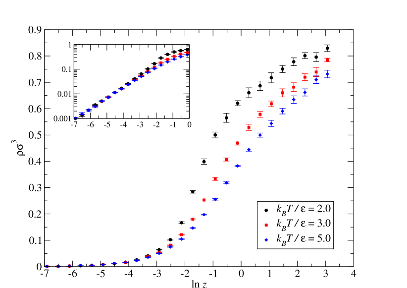
Figure 1: Isotherms for the Lennard-Jones fluid automatically generated using the simtask framework.

The most widely used model for fluids in molecular simulation is the Lennard-Jones fluid, a system of particles interacting via the Lennard-Jones potential

$$\phi(r)=4\epsilon\biggl{[}\Bigl{(}\frac{\sigma}{r}\Bigr{)}^{12}-\Bigl{(}\frac{\sigma}{r}\Bigr{)}^{6}\biggr{]},$$ (1)

where $\epsilon$ and $\sigma$ are the free parameters in the potential. Figure 1 shows the output of the simtask framework when tasked to evaluate the $k_{B}T/\epsilon=$2, 3 and 5 isotherms of the Lennard-Jones fluid, using GCMC in DL_MONTE as the underlying simulation method. The figure shows $\rho\sigma^{3}$ versus $\ln z$, where $z$ denotes the thermodynamic activity and $\rho$ denotes the density, i.e. the number of particles per unit volume. The framework was used to calculate $\rho\sigma^{3}$ at each set of thermodynamic parameters to a precision of 0.02. The Python code given in Figure 2 demonstrates how the framework was used to calculate each isotherms in Figure 1. This code was invoked in a directory containing DL_MONTE input files corresponding to a GCMC simulation at the target temperature.

⬇

import dlmontepython.simtask.dlmonteinterface as interface

1001import dlmontepython.simtask.task as task

import dlmontepython.simtask.measurement as measurement

1003import numpy as np

1005# Array containing thermodynamic activities to examine

activities = np.logspace(-3.0, 1.3333333333, 26)

1007# Threshold precision for density at each activity

density_prec = 0.02

1009# Volume used in the simulations (used to convert ’density_prec’

# to corresponding precision for number of molecules)

1011volume = 8.0**3

1013# Create interface to DL_MONTE executable

interface = interface.DLMonteInterface(”DLMONTE-SRL.X”)

1015

# Create class corresponding to property to measure

1017# (observable): the number of molecules, N, in the system.

# The density can be obtained from N by dividing it by

1019# ’volume’.

nmol_obs = task.Observable( (”nmol”,0) )

1021observables = [ nmol_obs ]

1023# Dictionary storing threshold precisions for observables,

# i.e. threshold precision for N

1025prec= { nmol_obs : density_prec*volume }

1027# Object defining nature of calculation at each activity

M = measurement.Measurement(

1029 interface, observables, precisions=prec)

1031# Object defining nature of calculations over all

# activities

1033MS = measurement.MeasurementSweep(

param=”molchempot”, paramvalues=activities,

1035 measurement_template=M, outputdir=”isotherm”)

1037# Invoke framework, generating output of N vs. activity

MS.run()

Figure 2: Python code used to generate an isotherm in Figure 1.

2.3 htk.multihistogram: Multiple histogram reweighting

simtask can be used to automatically generate data for specified thermodynamic parameters. We now turn to functionality of dlmontepython which enables one to make the most of such data.

Histogram reweighting[11] is a powerful method which allows simulation data obtained at certain thermodynamic parameters to be used to make predictions at nearby thermodynamic parameters not explored by the simulation. Single histogram reweighting[34] is the simplest incarnation of the method, and involves using data obtained from a single simulation. Multiple histogram reweighting (MHR)[35] is its generalisation in which data from multiple simulations at different thermodynamic parameters can be pooled and used to make predictions at thermodynamic parameters not explored by any of the simulations. We now describe the MHR functionality, which is housed in the htk.multihistogram module.

2.3.1 Methodology

The abstraction in this module is designed so that MHR can be applied to a wide range of thermodynamic ensembles – following the approach taken previously with the single histogram functionality[19]. To elaborate, a MHR function is provided for applying to thermodynamic ensembles with the general form

$$p_{i}\propto\exp(\mathbf{b}\cdot\mathbf{X}_{i}),$$ (2)

where $p_{i}$ is the probability of a configuration $i$, where $\mathbf{b}$ is a vector of thermodynamic parameters, $\mathbf{X}_{i}$ is a vector of physical quantities for $i$ ‘conjugate’ to those in $\mathbf{b}$, and ‘$\cdot$’ denotes the conventional dot product between a pair of vectors. This form covers the most common thermodynamic ensembles used in molecular simulation, including the canonical (constant number of particles $N$, volume $V$ and temperature $T$), isothermal-isobaric ($N$, pressure $P$, $T$) and grand-canonical (chemical potential $\mu$, $V$, $T$) ensembles. For example, in the grand-canonical ensemble

$$p_{i}\propto\exp\bigl{[}-(\beta E_{i}+\beta\mu N_{i})\bigr{]},$$ (3)

where $\beta\equiv 1/(k_{B}T)$, $E_{i}$ is the energy of configuration $i$, and $N_{i}$ is the number of particles in $i$. This can be recovered from the generalised ensemble [Eqn. (2)] by using the following definitions for $\mathbf{b}$ and $\mathbf{X}_{i}$:

$$\mathbf{b}=\bigl{(}-\beta,\beta\mu\bigr{)},\quad\mathbf{X}_{i}=(E_{i},N_{i}).$$ (4)

In other words, the above definitions for $\mathbf{b}$ and $\mathbf{X}_{i}$ retrieve the grand-canonical ensemble from the generalised ensemble.

MHR in the generalised ensemble described above entails using time series over $\mathbf{X}$ and some physical property of interest $O$, obtained from $N_{\text{sims}}$ simulations performed using thermodynamic parameters $\mathbf{b}_{1},\mathbf{b}_{2},\dotsc,\mathbf{b}_{N_{\text{sims}}}$, to determine the expected value of $O$ at another set of thermodynamic parameters $\mathbf{b}$. The workhorse function reweight_observable in htk.multihistogram performs such reweighting. However, for the convenience of users MHR functions are also provided for the canonical, grand-canonical, and isothermal-isobaric ensembles which take familiar quantities such as $E_{i}$ and $N_{i}$ as arguments, to save users from having to ’translate’ into the generalised ensemble. An example in the grand-canonical ensemble is given below.

2.3.2 Example: Interpolation of an isotherm

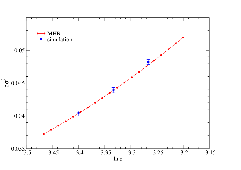
Figure 3: $k_{B}T/\epsilon=1.5$ isotherm for the Lennard-Jones fluid obtained by applying multiple histogram reweighting (MHR) to data from simulations performed at $\ln z=-3.40$, -3.33 and -3.27. The blue squares are the densities obtained directly from the simulations.

Figure 3 shows the results of applying MHR using htk.multihistogram to trace the $k_{B}T/\epsilon=1.5$ isotherm of the Lennard-Jones fluid between values of the thermodynamic activity, $z$, explored explicitly by GCMC simulations, namely $\ln z=-3.40$, $-3.33$ and $-3.27$. Details of the GCMC simulations are the same as given in Section 2.2.3. The Python code snippet given in Figure 4 demonstrates how the MHR isotherm in Figure 3 was generated.

⬇

import dlmontepython.htk.sources.dlmonte as dlmonte

1001import dlmontepython.htk.multihistogram as multihistogram

import numpy as np

1003

# List of directories containing DL_MONTE simulations at

1005# different chemical potentials or activities

simdirs = [ ”simdir_1”, ”simdir_2”, ”simdir_3” ]

1007

# List of chemical potentials to calculate density at

1009# using reweighting

mu_target = np.linspace(-5.2,-4.8,20)

1011

# Data and thermodynamic parameters for all simulations.

1013# kT[n] will be the temperature of simulation ’n’, and

# similarly for mu. E[n][i] will be the energy of

1015# simulation ’n’ at timestep ’i’, and similarly for

# N and rho.

1017kT, mu, E, N, rho = ([] for i in range(0,5))

1019# Import simulation data from directories, using classes

# in htk package to make importing easier.

1021for simdir in simdirs:

1023 dlminput = dlmonte.DLMonteInput.from_directory(simdir)

dlmoutput = dlmonte.DLMonteOutput.load(simdir)

1025

kT_sim = dlminput.control.temperature

1027 V_sim = dlminput.config.volume()

z_sim = dlminput.control.get_molecule_gcmc_potential(”lj”)

1029 mu_sim = np.log(z_sim)*kT_sim

1031 kT.append(kT_sim)

mu.append(mu_sim)

1033

E_sim = dlmoutput.yamldata.time_series(”energy”)

1035 N_sim = dlmoutput.yamldata.time_series(”nmol”)

N_sim = np.reshape(N_sim,len(N_sim))

1037 rho_sim = N_sim / V_sim

1039 E.append(E_sim)

N.append(N_sim)

1041 rho.append(rho_sim)

1043# Perform the reweighting and output

for mu_new in mu_target:

1045

rho_new = multihistogram.reweight_observable_muvt(

1047 kT, mu, E, N, rho, kT[0], mu_new)

1049 print(mu_new, rho_new)

Figure 4: Python code used to generate the multiple histogram reweighting isotherm in Figure 3.

2.4 fep: Reweighting and analysis of free energy profiles

2.4.1 Motivation

Free energy methods are a broad class of simulation methods which calculate the free energy profile $F(M)$ of a system over some order parameter or reaction coordinate $M$[4, 37]. An important application of free energy methods is to pinpoint the location of phase transitions[4], in particular the liquid-vapour transition in fluids and soft matter[38, 5, 6, 3, 39, 40]. This in turn enables related quantities such as the latent heat to be determined. Such free energy calculations involve first defining an order parameter $M$ such that, for some value $M_{\text{thresh}}$, $M<M_{\text{thresh}}$ corresponds to phase 1 and $M>M_{\text{thresh}}$ corresponds to phase 2. Locating the phase transition, i.e. where the two phases coexist, then entails calculating $F(M)$ at many thermodynamic parameters; one searches for the parameter at which the two phases have equal free energies – something which can be deduced from $F(M)$.

2.4.2 Functionality

The fep module was developed to assist with the types of calculations just described. In particular, for specific situations detailed in a moment, fep can exploit histogram reweighting to massively reduce the computational cost associated with locating coexistence. The underlying idea is that, given a $F(M)$ for a thermodynamic parameter close to coexistence, reweighting can be used to evaluate $F(M)$ at nearby parameters without the need for further costly ‘explicit’ calculations of $F(M)$.

The type of reweighting which is possible in the fep module is as follows. Consider the generalised thermodynamic ensemble described by Eqn. (2), in the special case where $M$ is one of the physical quantities in the vector $\mathbf{X}$. Let the thermodynamic parameter in $\mathbf{b}$ conjugate to $M$ (i.e. the $j$th element in $\mathbf{b}$ if $M$ is the $j$th element in $\mathbf{X}$) be denoted as $b$. Now, in this special case, if $b$ is the only parameter we wish to tune to obtain a new $F(M)$ via reweighting, then reweighting $F(M)$ becomes especially simple. The relevant equation is

$$F(M;b_{\text{new}})=-k_{B}T\ln\Biggl{\{}\int_{-\infty}^{\infty}dM\exp\Bigl{[}-F(M;b_{\text{old}})/(k_{B}T)+(b_{\text{new}}-b_{\text{old}})M\Bigr{]}\Biggr{\}},$$ (5)

where the reweighting is used to deduce the free energy profile at $b_{\text{new}}$ from the free energy profile $F(M;b_{\text{old}})$ at $b_{\text{old}}$. The function reweight can be used to apply the above equation. Moreover the function reweight_to_coexistence can be used to apply reweighting in a search for a value of $b$ which corresponds to coexistence, given $b_{\text{old}}$, $F(M;b_{\text{old}})$, a lower and upper bound of $b$ to use in the search, and a value for $M_{\text{thresh}}$ to define the order parameter ranges which correspond to phase 1 and phase 2.

The fep module also contains functions for extracting certain physical quantities from a free energy profile. As well as generic quantities such as the probabilities and expected values of $M$ for each phase, it also contains functions specific to the liquid-vapour problem. For instance, the functions vapour_pressure and surface_tension can be used to calculate, respectively, the pressure and surface tension from a free energy profile vs. number of molecules in the system[41, 42], as demonstrated in the following example.

2.4.3 Example: liquid-vapour coexistence properties of methane

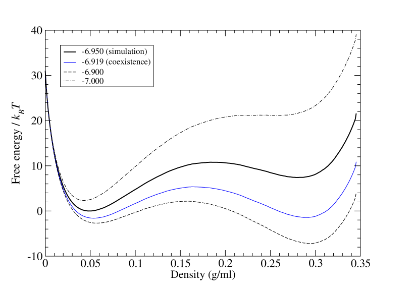
Figure 5: Free energy vs. density for methane modelled by the TraPPE-EH force field[43] at 175K and various $\ln z$. All curves were obtained by applying reweighting to the $\ln z=-6.950$ curve, which was obtained from simulation. -6.919 corresponds to liquid-vapour coexistence.

We have used fep to efficiently pinpoint liquid-vapour coexistence at 175K for methane modelled by the TraPPE-EH[43] force field. Moreover we also used fep to calculate the saturation pressure and liquid-vapour surface tension at this temperature. First, a free energy simulation (transition-matrix GCMC,[42] using DL_MONTE) was first performed at $\ln z=-6.950$. Figure 5 figure shows the free energy profile over the density – the relevant order parameter for the liquid-vapour problem – obtained from this simulation, as well as at nearby $\ln z$ obtained via reweighting using the fep module. The fep module was used to locate the $\ln z$ corresponding to coexistence. This was found to be $\ln z=-6.919$ and the free energy profile corresponding to this is also shown in the figure. Finally, using the free energy profile at coexistence, the saturation pressure and surface tension were calculated using the fep functions vapour_pressure and surface_tension, yielding 32.6 bar and 0.9 mNm^-1, respectively. The Python code used to generate Figure 5 is given in Figure 6.

⬇

import dlmontepython.fep.fep as fep

1001

# k_B*T used in simulation, units of kJ/mol

1003kt = 175 * 0.0083144621

# Value of ln(z) the simulation was performed at

1005lnz = -6.950

# Target ln(z) values for reweighting

1007lnz_target = [ -7.000, -6.900 ]

# Range of ln(z) to consider in search for coexistence

1009lnz_lbound = -7.0

lnz_ubound = -6.9

1011# Volume used in simulation (angstrom^3)

V = 30**3

1013# Molar mass of molecule (g/mol)

molarmass = 16.04

1015# Threshold between vapour and liquid densities (g/ml):

# systems with densities < rho_thresh are considered a vapour

1017rho_thresh = 0.17

1019# Name of file containing free energy profile vs. number

# of molecules

1021filename = ”FEDDAT.000_001”

1023# Import free energy profile over number of molecules

N, fe = fep.from_file(filename)

1025

# Output the free energy profile over the density

1027rho = N * molarmass / (V * 0.60221409)

fep.to_file(rho, fe, ”fep_vs_rho_”+str(lnz)+”_sim.dat”)

1029

# Reweight to target ln(z) and output

1031for lnz_new in lnz_target:

fe_new = fep.reweight(N, fe, lnz, lnz_new)

1033 fep.to_file(rho, fe_new, ”fep_vs_rho_”+str(lnz_new)+”.dat”)

1035# Locate coexistence ln(z) and output

N_thresh = rho_thresh * V * 0.60221409 / molarmass

1037lnz_co, p_co, fe_co = fep.reweight_to_coexistence(

N, fe, lnz, lnz_lbound, lnz_ubound,

1039 N_thresh)

fep.to_file(rho, fe_co, ”fep_vs_rho_”+str(lnz_co)+”_co.dat”)

1041

# Calculate cooexistence pressure ((kJ/mol)/A^3)

1043P = fep.vapour_pressure(N, fe_co, N_thresh, kt, V)

print(”coexistence pressure (bar) = ”, P * 1.0E5 / 6.02214076)

1045

# Calculate surface tension ((kJ/mol)/A^2)

1047A = V**(2.0/3.0)

tension = fep.surface_tension(N, fe_co, N_thresh, kt, A)

1049print(”surface tension (N/m) = ”, tension / 6.02214076)

Figure 6: Python code used to generate the free energy profiles in Figure 3.

3 Conclusions and Impact

We have described a Python library, dlmontepython, which has two overarching aims:

1. to facilitate the development of Python scripts which automate common simulation tasks, e.g. the calculation of an isotherm to a given precision;

2. to facilitate the application of data analysis methods pertinent to molecular simulation, especially Monte Carlo.

As well as providing an overview of key current functionality of the library, we also provided three examples to demonstrate its utility. Specifically, we used the library to automatically calculate isotherms to a specified precision; used histogram reweighting to interpolate isotherms between points explored by simulation; and used reweighting to pinpoint liquid-vapour coexistence and calculate the saturation pressure and surface tension for methane. These examples reflect common applications of Monte Carlo simulation. For example, such calculations are routinely employed in the development of accurate models for fluids, and in the design of new materials for energy applications. We therefore believe that dlmontepython will prove useful to practitioners of molecular simulation, especially those who use Monte Carlo simulation and DL_MONTE.

References

- [1] D. Frenkel, B. Smit, Understanding Molecular Simulation: From Algorithms to Applications, 2nd Edition, Academic Press, San Diego, 2002.
- [2] M. P. Allen, D. J. Tildesley, Computer Simulation of Liquids, Oxford University Press, USA, 1989.
- [3] D. Dubbeldam, A. Torres-Knoop, K. S. Walton, On the inner workings of Monte Carlo codes, Molecular Simulation 39 (14-15) (2013) 1253–1292. doi:10.1080/08927022.2013.819102.
- [4] A. D. Bruce, N. B. Wilding, Computational Strategies for Mapping Equilibrium Phase Diagrams, John Wiley & Sons, Ltd., 2004, Ch. 1, pp. 1–64. doi:10.1002/0471466603.ch1.
- [5] A. Panagiotopoulos, Monte Carlo methods for phase equilibria of fluids, Journal of Physics: Condensed Matter 12 (3) (2000) R25–R52. doi:{10.1088/0953-8984/12/3/201}.
- [6] J. de Pablo, Q. Yan, F. Escobedo, Simulation of phase transitions in fluids, Annual Review of Physical Chemistry 50 (1999) 377–411. doi:{10.1146/annurev.physchem.50.1.377}.
- [7] K. Binder, Monte Carlo Simulation in Statistical Physics : An Introduction, 5th Edition, Graduate Texts in Physics, Springer Berlin Heidelberg : Imprint: Springer, Berlin, Heidelberg, 2010.
- [8] C. J. Geyer, Practical Markov Chain Monte Carlo, Statistical Science 7 (4) (1992) 473–483.
- [9] J. D. Chodera, A simple method for automated equilibration detection in molecular simulations, Journal of Chemical Theory and Computation 12 (4) (2016) 1799–1805. doi:10.1021/acs.jctc.5b00784.
- [10] W. Yang, R. Bitetti-Putzer, M. Karplus, Free energy simulations: Use of reverse cumulative averaging to determine the equilibrated region and the time required for convergence, The Journal of Chemical Physics 120 (6) (2004) 2618–2628. doi:10.1063/1.1638996.
- [11] D. P. Landau, K. Binder, A Guide to Monte Carlo Simulations in Statistical Physics, 3rd Edition, Cambridge University Press, 2009. doi:10.1017/CBO9780511994944.
- [12] W. Smith, T. Forester, DL_POLY_2.0: A general-purpose parallel molecular dynamics simulation package, Journal of Molecular Graphics 14 (3) (1996) 136 – 141. doi:https://doi.org/10.1016/S0263-7855(96)00043-4.
- [13] I. T. Todorov, W. Smith, K. Trachenko, M. T. Dove, DL_POLY_3: new dimensions in molecular dynamics simulations via massive parallelism, Journal of Materials Chemistry 16 (2006) 1911–1918. doi:10.1039/B517931A.
- [14] J. C. Phillips, R. Braun, W. Wang, J. Gumbart, E. Tajkhorshid, E. Villa, C. Chipot, R. D. Skeel, L. Kalé, K. Schulten, Scalable molecular dynamics with NAMD, Journal of Computational Chemistry 26 (16) (2005) 1781–1802. doi:10.1002/jcc.20289.
- [15] R. Salomon-Ferrer, D. A. Case, R. C. Walker, An overview of the Amber biomolecular simulation package, WIREs Computational Molecular Science 3 (2) (2013) 198–210. doi:10.1002/wcms.1121.
- [16] B. R. Brooks, C. L. Brooks III, A. D. Mackerell Jr., L. Nilsson, R. J. Petrella, B. Roux, Y. Won, G. Archontis, C. Bartels, S. Boresch, A. Caflisch, L. Caves, Q. Cui, A. R. Dinner, M. Feig, S. Fischer, J. Gao, M. Hodoscek, W. Im, K. Kuczera, T. Lazaridis, J. Ma, V. Ovchinnikov, E. Paci, R. W. Pastor, C. B. Post, J. Z. Pu, M. Schaefer, B. Tidor, R. M. Venable, H. L. Woodcock, X. Wu, W. Yang, D. M. York, M. Karplus, CHARMM: The biomolecular simulation program, Journal of Computational Chemistry 30 (10) (2009) 1545–1614. doi:10.1002/jcc.21287.
- [17] S. Plimpton, Fast parallel algorithms for short-range molecular dynamics, Journal of Computational Physics 117 (1) (1995) 1 – 19. doi:https://doi.org/10.1006/jcph.1995.1039.
- [18] M. J. Abraham, T. Murtola, R. Schulz, S. Páll, J. C. Smith, B. Hess, E. Lindahl, GROMACS: High performance molecular simulations through multi-level parallelism from laptops to supercomputers, Software X 1-2 (2015) 19 – 25. doi:https://doi.org/10.1016/j.softx.2015.06.001.
- [19] A. V. Brukhno, J. Grant, T. L. Underwood, K. Stratford, S. C. Parker, J. A. Purton, N. B. Wilding, DL_MONTE: a multipurpose code for Monte Carlo simulation, Molecular Simulation (2019). doi:10.1080/08927022.2019.1569760.
- [20] M. G. Martin, MCCCS Towhee: a tool for Monte Carlo molecular simulation, Molecular Simulation 39 (14-15) (2013) 1212–1222. doi:10.1080/08927022.2013.828208.
- [21] J. K. Shah, E. Marin-Rimoldi, R. G. Mullen, B. P. Keene, S. Khan, A. S. Paluch, N. Rai, L. L. Romanielo, T. W. Rosch, B. Yoo, E. J. Maginn, Cassandra: An open source Monte Carlo package for molecular simulation, Journal of Computational Chemistry 38 (19) (2017) 1727–1739. doi:10.1002/jcc.24807.
- [22] D. Dubbeldam, S. Calero, D. E. Ellis, R. Q. Snurr, RASPA: molecular simulation software for adsorption and diffusion in flexible nanoporous materials, Molecular Simulation 42 (2) (2016) 81–101. doi:10.1080/08927022.2015.1010082.
- [23] A. Gupta, S. Chempath, M. J. Sanborn, L. A. Clark, R. Q. Snurr, Object-oriented programming paradigms for molecular modeling, Molecular Simulation 29 (1) (2003) 29–46. doi:10.1080/0892702031000065719.
- [24] J. A. Anderson, J. Glaser, S. C. Glotzer, HOOMD-blue: A python package for high-performance molecular dynamics and hard particle Monte Carlo simulations, Computational Materials Science 173 (2020) 109363. doi:https://doi.org/10.1016/j.commatsci.2019.109363.
- [25] J. Purton, J. Crabtree, S. Parker, DL_MONTE: a general purpose program for parallel Monte Carlo simulation, Molecular Simulation 39 (14-15) (2013) 1240–1252. doi:10.1080/08927022.2013.839871.
- [26] A. Hjorth Larsen, J. Jørgen Mortensen, J. Blomqvist, I. E. Castelli, R. Christensen, M. Dułak, J. Friis, M. N. Groves, B. Hammer, C. Hargus, E. D. Hermes, P. C. Jennings, P. Bjerre Jensen, J. Kermode, J. R. Kitchin, E. Leonhard Kolsbjerg, J. Kubal, K. Kaasbjerg, S. Lysgaard, J. Bergmann Maronsson, T. Maxson, T. Olsen, L. Pastewka, A. Peterson, C. Rostgaard, J. Schiøtz, O. Schütt, M. Strange, K. S. Thygesen, T. Vegge, L. Vilhelmsen, M. Walter, Z. Zeng, K. W. Jacobsen, The atomic simulation environment – a Python library for working with atoms, Journal of Physics: Condensed matter 29 (27) (2017) 273002.
- [27] N. Michaud-Agrawal, E. J. Denning, T. B. Woolf, O. Beckstein, MDAnalysis: A toolkit for the analysis of molecular dynamics simulations, Journal of Computational Chemistry 32 (10) (2011) 2319–2327. doi:10.1002/jcc.21787.
- [28] Richard J. Gowers, Max Linke, Jonathan Barnoud, Tyler J. E. Reddy, Manuel N. Melo, Sean L. Seyler, Jan Domański, David L. Dotson, Sébastien Buchoux, Ian M. Kenney, Oliver Beckstein, MDAnalysis: A Python Package for the Rapid Analysis of Molecular Dynamics Simulations, in: Sebastian Benthall, Scott Rostrup (Eds.), Proceedings of the 15th Python in Science Conference, 2016, pp. 98 – 105. doi:10.25080/Majora-629e541a-00e.
- [29] https://gitlab.com/dl_monte/dlmontepython.
- [30] T. Kluyver, B. Ragan-Kelley, F. Pérez, B. E. Granger, M. Bussonnier, J. Frederic, K. Kelley, J. B. Hamrick, J. Grout, S. Corlay, P. Ivanov, D. Avila, S. Abdalla, C. Willing, et al., Jupyter notebooks - a publishing format for reproducible computational workflows, in: ELPUB, 2016.
- [31] P. Virtanen, R. Gommers, T. E. Oliphant, M. Haberland, T. Reddy, D. Cournapeau, E. Burovski, P. Peterson, W. Weckesser, J. Bright, S. J. van der Walt, M. Brett, J. Wilson, K. Jarrod Millman, N. Mayorov, A. R. J. Nelson, E. Jones, R. Kern, E. Larson, C. Carey, İ. Polat, Y. Feng, E. W. Moore, J. Vand erPlas, D. Laxalde, J. Perktold, R. Cimrman, I. Henriksen, E. A. Quintero, C. R. Harris, A. M. Archibald, A. H. Ribeiro, F. Pedregosa, P. van Mulbregt, SciPy 1.0 Contributors, SciPy 1.0: Fundamental Algorithms for Scientific Computing in Python, Nature Methods 17 (2020) 261–272. doi:https://doi.org/10.1038/s41592-019-0686-2.
- [32] C. R. Harris, K. J. Millman, S. J. van der Walt, R. Gommers, P. Virtanen, D. Cournapeau, E. Wieser, J. Taylor, S. Berg, N. J. Smith, R. Kern, M. Picus, S. Hoyer, M. H. van Kerkwijk, M. Brett, A. Haldane, J. F. del R’ıo, M. Wiebe, P. Peterson, P. G’erard-Marchant, K. Sheppard, T. Reddy, W. Weckesser, H. Abbasi, C. Gohlke, T. E. Oliphant, Array programming with NumPy, Nature 585 (7825) (2020) 357–362. doi:10.1038/s41586-020-2649-2.
- [33] https://pypi.org/project/dlmontepython.
- [34] A. M. Ferrenberg, R. H. Swendsen, New Monte Carlo technique for studying phase transitions, Physical Review Letters 61 (1988) 2635–2638. doi:10.1103/PhysRevLett.61.2635.
- [35] A. M. Ferrenberg, R. H. Swendsen, Optimized Monte Carlo data analysis, Physical Review Letters 63 (1989) 1195–1198. doi:10.1103/PhysRevLett.63.1195.
- [36] S. Kumar, J. M. Rosenberg, D. Bouzida, R. H. Swendsen, P. A. Kollman, The weighted histogram analysis method for free-energy calculations on biomolecules. i. the method, Journal of Computational Chemistry 13 (8) (1992) 1011–1021. doi:10.1002/jcc.540130812.
- [37] S. Singh, M. Chopra, J. J. de Pablo, Density of States-Based Molecular Simulations, Annual Review of Chemical and Biomolecular Engineering 3 (1) (2012) 369–394. doi:10.1146/annurev-chembioeng-062011-081032.
- [38] N. B. Wilding, Computer simulation of fluid phase transitions, American Journal of Physics 69 (11) (2001) 1147–1155. doi:10.1119/1.1399044.
- [39] A. Broukhno, Free energy and surface forces in polymer systems: Monte Carlo simulation studies, Ph.D. thesis, Lund University (2003).
- [40] A. V. Brukhno, T. Åkesson, B. Jönsson, Phase behavior in suspensions of highly charged colloids, The Journal of Physical Chemistry B 113 (19) (2009) 6766–6774.
- [41] J. R. Errington, A. Z. Panagiotopoulos, Phase equilibria of the modified Buckingham exponential-6 potential from Hamiltonian scaling grand canonical Monte Carlo, The Journal of Chemical Physics 109 (3) (1998) 1093–1100. doi:10.1063/1.476652.
- [42] J. R. Errington, Evaluating surface tension using grand-canonical transition-matrix Monte Carlo simulation and finite-size scaling, Physical Review E 67 (2003) 012102. doi:10.1103/PhysRevE.67.012102.
- [43] B. Chen, J. I. Siepmann, Transferable potentials for phase equilibria. 3. explicit-hydrogen description of normal alkanes, The Journal of Physical Chemistry B 103 (25) (1999) 5370–5379. doi:10.1021/jp990822m.