Strong coupling methods in QCD thermodynamics

Abstract

For a long time, strong coupling expansions have not been applied systematically in lattice QCD thermodynamics, in view of the succes of numerical Monte Carlo studies. The persistent sign problem at finite baryo-chemical potential, however, has motivated investigations using these methods, either by themselves or combined with numerical evaluations, as a route to finite density physics. This article reviews the strategies, by which a number of qualitative insights have been attained, notably the emergence of the hadron resonance gas or the identification of the onset transition to baryon matter in specific regions of the QCD parameter space. For the simpler case of Yang-Mills theory, the deconfinement transition can be determined quantitatively even in the scaling region, showing possible prospects for continuum physics.

1 Introduction

Quantum Chromodynamics (QCD) at finite temperatures and baryon densities is the theoretical foundation for an understanding of observed phenomena in a wide range of fields, like the thermal history of the early universe, heavy-ion collision experiments or the composition and properties of neutron stars. Since the interactions of QCD are strong on scales up to several GeV, ordinary weak coupling perturbation theory fails for temperatures and baryo-chemical potentials $T,\mu_{B}\raise 1.29167pt\hbox{$<$\kern-7.5pt\raise-4.73611pt\hbox{$\sim$}}2$ GeV. The non-perturbative treatment by numerical Monte Carlo simulations of lattice QCD is to date still restricted to vanishing or small baryo-chemical potentials, because of a severe sign problem at finite baryon density (for an introduction, see Philipsen:2010gj ).

The continued absence of a genuine algorithmic solution to this problem has motivated renewed interest in strong coupling and hopping expansion methods over the last decade. Contrary to weak coupling expansions, which typically result in asymptotic series, strong coupling expansions in the Euclidean framework are known to yield convergent series with well-defined radii of convergence. In the early days of lattice gauge theory they were used to get analytical results for some physical quantities of interest, such as glueball masses Munster:1981es ; Seo:1982jh or the energy density of lattice Yang-Mills theories Balian:1974xw ; Drouffe:1983fv . These calculations were restricted to zero temperature, with the exception of some mean field analyses of phase transitions in the strong coupling limit Polonyi:1982wz ; Green:1983bq ; Green:1983sd ; Gocksch:1984xc , and a series for the temperature-dependent string tension Green:1982hu . More recent attempts to explore strong coupling methods as a systematic calculational tool for thermodynamics started with an investigation of Yang-Mills theory Langelage:2008dj . While Monte Carlo methods appear superior where they work, analytic results provide additional understanding for the interpretation of data. Moreover a two-stage approach, with an analytic derivation of effective lattice theories and their subsequent analytic or numerical solution, appears to be reasonably promising for finite baryon density. It is currently the only way to investigate the onset transition to baryon matter in lattice QCD directly, albeit not yet for physical parameter values. The purpose of this article is to review these developments with a focus on the concepts and the results, whereas technical details are left to the references.

2 A proof of concept: the $SU(3)$ spin model

Before approaching the difficulty and complexity of QCD, it is useful to illustrate the basic strategies at the example of a simpler theory that is fully understood and has served several times as a testing ground for methods to deal with the sign problem. We consider the $SU(3)$ spin model with the action

$$S=-\sum_{x}\Big{(}\sum_{k=1}^{3}\tau\left[L(x)L^{*}(x+\hat{k})+L^{*}(x)L(x+\hat{k})\right]+\eta L(x)+\bar{\eta}L^{*}(x)\Big{)}.$$ (1)

The fields $L(x)={\rm Tr}W(x)$ are complex scalars representing the trace of $SU(3)$-matrices $W(x)$. Writing $\eta=\kappa\exp(\mu),\bar{\eta}=\eta(-\mu)$, the model closely resembles an effective action of lattice QCD with static quarks in the strong coupling region, to be discussed in Sec. 4. For $\mu=0$, it features spontaneous breaking of its $Z(3)$ center symmetry along a line $\tau_{c}(\kappa)$ of first-order transitions with an endpoint, as well as a sign problem at $\mu\neq 0$. The model can be reformulated free of a sign problem in terms of a flux representation Gattringer:2011gq , allowing for simulations Mercado:2012ue by means of a worm algorithm. Likewise, a complex Langevin algorithm has been successfully applied Karsch:1985cb ; Bilic:1987fn ; Aarts:2011zn .

Here, we are interested in a solution by series expansion methods, which are more familiar in condensed matter physics. Specifically, consider a linked cluster expansion of the free energy density (for an introduction, see Wortis:1980zc ), which has been evaluated through 14 orders in $\tau$, and for each order up to convergence in $\kappa$ Kim:2020atu ,

$$f=-\frac{\ln(Z)}{V}=\sum_{n=0}^{14}a_{n}(\kappa,\mu)\tau^{n}\;,\quad\Delta S=-\frac{\partial f}{\partial\tau}-\frac{\partial f}{\partial\eta}\;.$$ (2)

The equation of state can be parametrised by the combined derivatives $\Delta S$, corresponding to the interaction measure in QCD. It can be straightforwardly determined in Monte Carlo simulations, and all thermodynamic functions follow by integration or differentiation. Results corresponding to the three highest orders are shown in Fig. 1 (left). Excellent convergence and agreement with Monte Carlo results is observed until the phase transition, representing the radius of convergence, is approached. A finite polynomial is unable to describe a non-analytic phase transition, but is sensitive to it by loss of convergence.

A marked improvement near the transition can be obtained by infinite-order resummations through Padé approximants, defined as rational functions,

$$[L,M](x)\equiv\frac{a_{0}+a_{1}x+\ldots+a_{L}x^{L}}{1+b_{1}x+\ldots+b_{M}x^{M}}\;.$$ (3)

The coefficients $a_{i},b_{i}$ are uniquely determined for $L+M\leq N$, if $N$ represents the highest available order of the expansion. In this way the $[L,M]$ approximant reproduces the known series up to and including $\mathcal{O}(x^{L+M})$. Padé approximants are able to show singular behaviour and can model scaling properties near second-order phase transitions. The $[6,6]$ approximant to $\Delta S$ is shown also in Fig. 1 (left). It accurately reproduces the simulated equation of state all the way to the phase transition, which it indicates by a singularity.

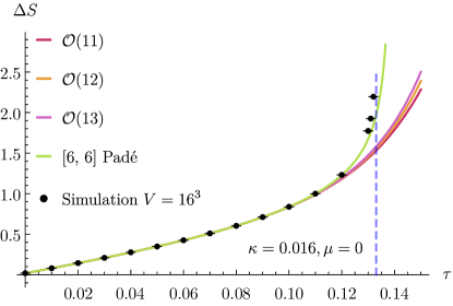
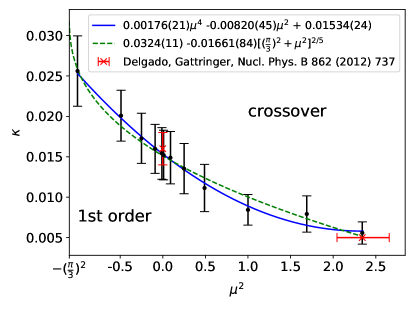
Figure 1: Equation of state from the linked cluster expansion compared to Monte Carlo. The vertical line marks the center breaking phase transition. Right: Order of the phase transitions, at an implicit $\tau_{c}(\kappa,\mu)$, in the $SU(3)$ spin model. First-order and crossover regions are separated by a critical line with 3d $Z(2)$ universality. From Kim:2020atu .

At $\mu=0$ the phase transition is known to be first-order for small $\kappa$, ending in a critical point at some $\kappa_{c}$, which is of the same type as standard liquid-gas transitions. Therefore the susceptibility and the specific heat,

$$\chi=-\frac{\partial^{2}f}{\partial\eta^{2}}-\frac{\partial^{2}f}{\partial\bar{\eta}^{2}}-2\frac{\partial^{2}f}{\partial\eta\partial\bar{\eta}}\;,\quad C=-\frac{\partial^{2}f}{\partial\tau^{2}}\;,$$ (4)

when approaching from any direction not parallel to the scaling axes, must both diverge with a common critical exponent, $\chi\sim C\sim|\tau-\tau_{c}|^{-\epsilon}$, $\epsilon=\gamma/\beta\delta$. This is reflected in a simple pole of the Dlog-Padé’s, e.g.,

$$D_{\chi}(\tau)\equiv\frac{d}{d\tau}\log\chi\sim-\frac{\epsilon}{(\tau-\tau_{c})}\;.$$ (5)

A difficulty is that Padé’s also show poles for first-order transitions, where they indicate the end of the metastability range, as well as spurious poles, which renders the analysis quite intricate. In order to detect a true critical point one has to require convergence of the poles predicted by different Padé’s, as well as convergence of he poles in both observables, $D_{\chi},D_{C}$. In this way, a critical point can be located within some scatter specifying a systematic error. Once the series are long enough to achieve this, an application to finite chemical potential, real or imaginary, poses no additional problem. Hence, the phase structure and the order of the phase tansition can be fully determined, as shown in Fig. 1 (right), in quantitative agreement with numerical results. This example provides further motivation to explore such methods also in QCD, where no algorithmic solutions to the sign problem exist yet.

3 Strong coupling and hopping expansions in QCD at finite T

3.1 Yang-Mills theory

Consider the Yang-Mills partition function with the standard Wilson action

$$Z=\int\,DU\,\exp-S_{YM}[U],\quad S_{\mathrm{YM}}=\sum_{p}\frac{\beta}{2N_{c}}\left(\mathrm{Tr}\,U_{p}+\mathrm{Tr}\,U_{p}^{\dagger}\right),$$ (6)

with plaquette variables $U_{p}$ and the lattice coupling $\beta=\frac{2N_{c}}{g^{2}}$. From the lattice action it is obvious that the exponential can be expanded in powers of $\beta$, where the expansion point $\beta=0$ corresponds to the strong (infinite) coupling limit. However, in the continuum limit $\beta\rightarrow\infty$ and convergence is expected to be slow. A powerful resummation including all orders in $\beta$ is immediately achieved by expanding instead in the group characters $\chi_{r}(U_{p})={\rm Tr}D_{r}(U_{p})$, which are traces of the representation matrices $D_{r}$ of the plaquette variables. Using the formalism of moments and cumulants Drouffe:1983fv ; Montvay:1994cy , it can be shown that this expansion exponentiates, such that a series for the (formal) free energy density $\tilde{f}\equiv-\frac{1}{\Omega}\ln Z$ is obtained in terms of clusters $C$ of graphs $\Phi$,

$$\tilde{f} = -6\ln\,c_{0}(\beta)-\frac{1}{\Omega}\sum_{C=(X_{i}^{n_{i}})}\,a(C)\prod_{i}\Phi(X_{i})^{n_{i}}\;,$$

$$\Phi(X_{i}) = \int DU\prod_{p\in X_{i}}d_{r}a_{r}(\beta)\chi_{r}(U_{p})\;.$$ (7)

Here $\Omega=V\cdot N_{\tau}$ is the lattice volume, $d_{r}$ and $a_{r}(\beta)$ are the dimension and expansion coefficient of representation $r$, and $c_{0}$ is the expansion coefficient of the trivial representation. The combinatorial factor $a(C)$ equals $1$ for clusters $C$ consisting of only one so-called polymer $X_{i}$, which represent closed surfaces of plaquettes. The coefficients of higher representations can be expressed in terms of $u(\beta)\equiv a_{f}(\beta)=\beta/18+\beta^{2}/216+\ldots$, the coefficient of the fundamental representation. It is a known function over the entire range of lattice gauge couplings with $u(\beta)\in[0,1)$, and constitutes the expansion parameter for the character expansion.

For thermodynamics the physical temperature $T=1/(aN_{\tau})$ is realised by compactifying the temporal extension of the lattice. The physical free energy is then obtained by subtracting the divergent vacuum contribution,

$$f(N_{\tau},u)=\tilde{f}(N_{\tau},u)-\tilde{f}(\infty,u),$$ (8)

and the pressure is $P=-f$. Group integrals are evaluated using the formulae

$$\int dU\chi_{r}(UV)\chi_{r}(WU^{-1})=\chi_{r}(VW),\quad\int dU\chi_{r}(U)=\delta_{r,0},$$ (9)

the latter enforces contributing graphs $X_{i}$ to be objects with a closed surface.

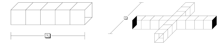
Figure 2: Leading order graphs for the free energy density (left) and screening mass (right).

The leading order graph is a tube of length $N_{\tau}$, Fig. 2. Summing over all such graphs on the lattice, their contribution to the pressure is

$$P^{LO}(N_{\tau},u)=\frac{6}{N_{\tau}}u^{4N_{\tau}}\;.$$ (10)

Thus, the strong coupling limit at $\beta=0$ (and thus $T=0$) has zero free enery density or pressure, as expected. Moreover, we recognize a qualitative feature known from full lattice simulations, where it is difficult to extract, and hadron resonance gas descriptions, namely the exponentially slow rise of the pressure with $T$. In order to get more quantitative, corrections to the free energy density through order $u^{8}$ with respect to the leading order term for various $N_{\tau}$ have been calculated for SU(2) Langelage:2008dj and for SU(3) Langelage:2009jb ; Langelage:2010yn . A direct comparison with Monte Carlo simulations is easiest for the energy density,

$$e(\beta)=\frac{1}{6}\frac{d}{d\beta}f(\beta)=\langle\,{\rm Tr}\,U_{p}\,\rangle_{N_{\tau}}-\langle\,{\rm Tr}\,U_{p}\,\rangle_{N_{\tau}=\infty},$$ (11)

which is shown in Fig. 3 for the example of $SU(2)$. On the left, the series is shown order by order in the character coefficient $u(\beta)$, and evaluated as a function of $\beta$. The series loses convergence as it approaches the deconfinement transition, whose critical coupling $\beta_{c}$ bounds the radius of convergence in this case. On the right, a resummation of the series is achieved by Padé approximants. This clearly improves the convergence and comparsion between different approximants provides an estimate for the systematic error associated with the truncated series. Good agreement with the Monte Carlo data is observed in the controlled region, which is however restricted to relatively small $\beta$-values.

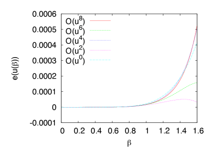
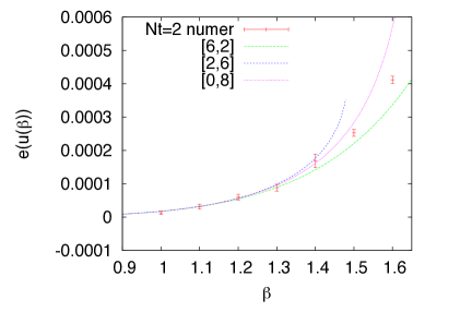
Figure 3: Left: Energy density to different orders in the character expansion. Right: Resummation by Padé approximants and comparison with Monte Carlo. From Langelage:2008dj .

At the finite temperature phase transition the free energy $f(N_{\tau},u(\beta_{c}))$ is continuous, with a discontinuous first or second derivative, depending on the order of the transition. For $SU(2)$, we have a second-order transition, for which the ‘heat capacity’

$$C(N_{\tau},u)=u^{2}\frac{d^{2}}{du^{2}}f(N_{\tau},u)$$ (12)

diverges as $C(u)\sim(u_{c}-u)^{\alpha}$, with a critical exponent characteristic of the universality class. Its logarithmic derivative

$$D_{C}(N_{\tau},u)\equiv\frac{d}{du}\ln C(N_{\tau},u)\sim-\frac{\alpha}{u_{c}-u}$$ (13)

has a simple pole with residue $\alpha$ and is therefore well-suited for an analysis by Padé approximants. The averaged predictions of the approximants in Fig. 3 are $\beta_{c}=1.65(35)$ and $\alpha=0.052(19)$ Langelage:2008dj , compared to the Monte Carlo value $\beta_{c}=1.880(3)$ Fingberg:1992ju and the 3d Ising exponent $\alpha=0.12$.

Another interesting qualitative result can be obtained for thermal screening masses, which are obtained from the exponential decay of spatial correlation functions. The correlator of plaquettes is given by

$$C(z)=\langle\mathrm{Tr}\,U_{p_{1}}(0)\,\,\mathrm{Tr}\,U_{p_{2}}(z)\rangle=N^{2}\frac{\partial^{2}}{\partial\beta_{1}\partial\beta_{2}}\ln\,Z(\beta,\beta_{1}\beta_{2})\bigg{|}_{\beta_{1,2}=\beta}.$$ (14)

At zero temperature (infinite $N_{\tau}$) the exponential decay is the same as for correlations in the time direction, and thus determined by the glueball masses. At finite temperature (finite $N_{\tau}$) the LO graph for the difference to the vacuum mass is shown in Fig. 2 (right) and gives

$$\Delta m^{LO}(N_{\tau},u)=m(N_{\tau})-m(\infty)=-\frac{2}{3}N_{\tau}u^{4N_{\tau}-6}\;.$$ (15)

Thus finite temperature lowers the screening mass in the confined phase, but the effect is suppressed by its high order in the expansion parameter. This explains the insensitiviy of screening masses to $T$ observed in simulations of the confined phase, where they stay very close to the vacuum hadron masses up to the phase transition Datta:2002je . Such an understanding is not attainable from simulations alone.

3.2 QCD with heavy quarks

Including fermions for a treatment of full QCD requires an additional expansion. The Wilson fermion determinant can be formulated as a power series in the hopping parameter $\kappa_{f}=(2am_{f}+8)^{-1}$ for every flavour $f$. Defining the usual hopping matrix $M$ in Dirac, colour and coordinate space, Grassmann integration over fermion fields gives to leading order in $\kappa_{f}$ per flavour

$$-S_{q}^{f} = -{\rm Tr}\,\ln\,(1-\kappa_{f}M)=\sum_{l}\,\frac{\kappa_{f}^{l}}{l}\,\mathrm{tr}\,M^{l}(\mu)$$ (16)

$$= -(2\kappa_{f})^{N_{\tau}}\sum_{\bf x}\left(e^{\mu N_{\tau}}L({\bf x})+e^{-\mu N_{\tau}}L^{\dagger}({\bf x})\right)+\ldots$$

$$\mbox{with}\quad M_{ab,\alpha\beta,yx} = \sum_{\mu}\delta_{y,x+\hat{\mu}}(1+\gamma_{\mu})_{\alpha\beta}U_{ab,x\mu}\;.$$ (17)

The Kronecker deltas in $M$ ensure that only closed loops contribute, and $l$ counts their length. Again, for finite temperature effects we only need the difference between finite and infinite $N_{\tau}$, and hence are interested in the loops winding through the temporal boundary. One can formalise this by considering a hopping expansion in the spatial directions only, while the hops in the Euclidean time direction are taken into account fully. Thus the leading order heavy fermionic contributions to the effective action can be written as in Eq. (16), which only holds for finite $T$, and the dots represent loops that wind more than once.

Now one can calculate again the free energy density and pressure, this time performing character expansions in both $U$ and $L$. Expanding all terms up to ${\cal{O}}(\kappa^{3N_{\tau}})$ and doing the group integrals one finds for two flavours $u,d$ Langelage:2010yn

$$P = \frac{1}{N_{\tau}a^{4}}\bigg{\{}4(2\kappa_{u})^{2N_{\tau}}+8(2\kappa_{u}2\kappa_{d})^{N_{\tau}}+4(2\kappa_{d})^{2N_{\tau}}\bigg{\}}$$ (18)

$$+ \frac{1}{N_{\tau}a^{4}}\bigg{\{}4(2\kappa_{u})^{3N_{\tau}}+6\big{[}(2\kappa_{u})^{2}2\kappa_{d}\big{]}^{N_{\tau}}$$

$$+ 6\big{[}2\kappa_{u}(2\kappa_{d})^{2}\big{]}^{N_{\tau}}+4(2\kappa_{d})^{3N_{\tau}}\bigg{\}}\Big{(}\mathrm{e}^{3a\mu N_{\tau}}+\mathrm{e}^{-3a\mu N_{\tau}}\Big{)}\;.$$

Next we identify the hadron masses to leading order in the hopping expansion,

$$\mbox{Mesons:}\qquad\quad am_{f\bar{f^{\prime}}} = -\ln 2\kappa_{f}-\ln 2\kappa_{f^{\prime}}$$ (19)

$$\mbox{Baryons:}\qquad am_{ff^{\prime}f^{\prime\prime}} = -\ln 2\kappa_{f}-\ln 2\kappa_{f^{\prime}}-\ln 2\kappa_{f^{\prime\prime}}.$$ (20)

The pressure can then be rewritten as

$$P = \frac{1}{N_{\tau}a^{4}}\left\{\sum_{0^{-}}\mathrm{e}^{-m\left(0^{-}\right)N_{\tau}}+3\sum_{1^{-}}\mathrm{e}^{-m\left(1^{-}\right)N_{\tau}}\right\}$$ (21)

$$+ \frac{1}{N_{\tau}a^{4}}\Bigg{\{}4\sum_{\frac{1}{2}^{+}}\mathrm{e}^{-m\left(\frac{1}{2}^{+}\right)N_{\tau}}+8\sum_{\frac{3}{2}^{+}}\mathrm{e}^{-m\left(\frac{3}{2}^{+}\right)N_{\tau}}\Bigg{\}}\cosh\big{(}\mu_{B}N_{\tau}\big{)},$$

which is the expression corresponding to an ideal gas of hadrons. We have thus derived from first principles that QCD reduces to a hadron resonance gas in the strong coupling and heavy mass regime. Note that this also holds for Yang-Mills theory, which can be represented as a glueball gas Langelage:2008dj ; Langelage:2010yn . It is then plausible that this feature is generic and independent of quark mass, which explains the success of hadron resonance gas descriptions of the lattice QCD equation of state in the confined phase, where the physical gauge coupling is fairly strong Borsanyi:2010cj ; Bazavov:2014pvz .

3.3 Effective lattice theories from strong coupling methods

In the previous section we have seen that strong coupling methods lead to interesting qualitative insights in QCD thermodynamics, but they are also limited quantitatively if we are interested in continuum physics. This can be improved significantly by a procedure in two stages: 1) construct an effective lattice theory by integrating out part of the degrees of freedom, and 2) solve the effective theory by series expansion or otherwise. Two types of effective degrees of freedom arise naturally, depending on the integration order,

$$Z=\int DUD\bar{\psi}D\psi\;e^{-S_{\mathrm{QCD}}[U,\bar{\psi},\psi]}=\int DU_{0}\;e^{-S_{\mathrm{eff}}[U_{0}]}=\int D\bar{\psi}D\psi\;\;e^{-S_{\mathrm{eff}}[\bar{\psi},\psi]}\;.$$ (22)

In the first case, fermions as well as all spatial link variables are integrated over, leaving a theory of temporal links only, which on a periodic lattice can be expressed by Polyakov loops. In the second case, all gauge links are integrated, leaving a fermionic effective theory in terms of mesons and baryons, because of gauge invariance. Both representations are perfectly equivalent to QCD. Truncations involved in doing the integrations reduce this equivalence to specific parameter regions, where the corresponding approximations hold.

4 Effective lattice theory for QCD with heavy quarks

The representation of QCD in terms of Polyakov loops was first developed to characterise the deconfinement phase transition in pure gauge theories Polonyi:1982wz ; Svetitsky:1982gs , and has later been considered perturbatively and non-perturbatively in the continuum Herbst:2013ufa ; Vuorinen:2006nz ; Fischer:2013eca ; Fischer:2014vxa ; Lo:2014vba and on the lattice Wozar:2007tz ; Greensite:2013yd ; Greensite:2013bya ; Greensite:2014isa ; Bergner:2015rza . Here our interest is in the derivation of the effective theories by strong coupling methods. In this case their form is uniquely determined and can be systematically worked out and improved. Starting point is Wilson’s lattice formulation, as before. However, instead of the free energy we now compute the effective action defined in the first of Eq. (22),

$$-S_{\mathrm{eff}}[U_{0}]\equiv\ln\int DU_{i}\exp(-S_{\mathrm{YM}}[U_{0},U_{i}]-S_{q}^{f}[U_{0},U_{i}])\;.$$ (23)

This is done again by combining a character expansion of the exponentiated gauge action with a hopping expansion of the exponentiated quark action. The gauge integrals can then be done term by term for the truncated expansion to leave an effective action depending on temporal links only. These combine to temporal Wilson lines $W({\bf x})$, which close through the periodic boundary and implicitly contain the dependence on the Euclidean time extent $N_{\tau}$. As a result, the effective partition function is three-dimensional, resembling a continuous spin model Langelage:2010yr ; Fromm:2011qi ,

$$Z = \int DW\prod_{<{\bf x},{\bf y}>}\left[1+\lambda(L_{{\bf x}}L_{{\bf y}}^{*}+L_{{\bf x}}^{*}L_{{\bf y}})\right]$$ (25)

$$\times\prod_{{\bf x}}[1+h_{1}L_{{\bf x}}+h_{1}^{2}L_{{\bf x}}^{*}+h_{1}^{3}]^{2N_{f}}[1+\bar{h}_{1}L^{*}_{{\bf x}}+\bar{h}_{1}^{2}L_{{\bf x}}+\bar{h}_{1}^{3}]^{2N_{f}}$$

$$\times\prod_{<{\bf x},{\bf y}>}\Big{(}1-h_{2}{\rm Tr}\frac{h_{1}W_{{\bf x}}}{1+h_{1}W_{{\bf x}}}{\rm Tr}\frac{h_{1}W_{{\bf y}}}{1+h_{1}W_{{\bf y}}}\Big{)}\Big{(}1-h_{2}{\rm Tr}\frac{\bar{h}_{1}W^{\dagger}_{{\bf x}}}{1+\bar{h}_{1}W^{\dagger}_{{\bf x}}}{\rm Tr}\frac{\bar{h}_{1}W^{\dagger}_{{\bf y}}}{1+\bar{h}_{1}W^{\dagger}_{{\bf y}}}\Big{)}$$

$$\times\quad\ldots\;\quad.$$

Here the first line corresponds to pure gauge theory, the second line to the static quark determinant and the third line to the leading contributions of the kinetic quark determinant. The couplings of the effective theory are functions of the original lattice QCD parameters (for higher order expressions see Fromm:2011qi ),

$$\lambda = u^{N_{\tau}}\exp[N_{\tau}(4u^{4}+\ldots)]\;,$$

$$h_{1} = (2\kappa e^{a\mu})^{N_{\tau}}\left(1+\ldots\right)=e^{\frac{\mu-m}{T}}(1+\ldots),\quad\bar{h}_{1}=h_{1}(-\mu)\;,$$

$$h_{2} = \kappa^{2}N_{\tau}/N_{c}(1+\ldots)\;.$$ (26)

and $am=-\ln(2\kappa)=am_{B}/3$ denotes the leading-order constituent quark mass in a baryon (not to be confused with the current quark mass $m_{q}$ in the QCD action). The higher the order to which the effective action is considered, the more couplings appear which are increasingly non-local, connecting loops $W_{\bf x}$ to all powers and over all lattice separations. Note that the effective couplings are (resummed) power series in the original expansion parameters $u$ and $\kappa$, and hence can in turn be treated as small expansion parameters themselves. Any truncated effective theory can thus be treated by series expansion methods as discussed in the simple example of Sec.2. On the other hand, the effective theory has a much reduced sign problem, and can be simulated by even a choice of different algorithms. One current line of work is to design flux representations for this type of actions that can cure the sign problem and be simulated efficiently Borisenko:2020gjn ; Borisenko:2020cjx .

4.1 Deconfinement transition in Yang-Mills theory

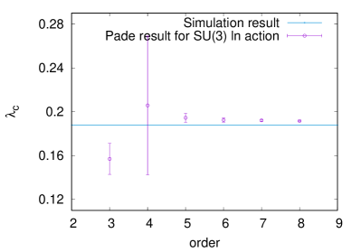
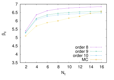
Figure 4: Left: Critical coupling of the effective lattice theory representing $SU(3)$ Yang-Mills. Right: Critical Yang-Mills couplings predicted by the effective theory, compared to Monte Carlo results. From Kim:2019ykj .

To appreciate the advantage of going through an effective theory, let us consider $SU(3)$ Yang-Mills theory, so that $h_{1}=\bar{h}_{1}=h_{2}=0$ and Eq. (25) is reduced to the first line. One can now compute the free energy and the susceptiblitiy of the Polyakov loop as a power series in $\lambda$, and improve the results by Padé approximants as in Sec. 3.1. These show a singularity at a critical $\lambda_{c}$, indicating the phase transition. Note however, that for $SU(3)$ we have a first-order phase transition, so that the singularity corresponds to the end of the metastability region of the disordered phase, i.e., the true critical coupling is slightly overestimated. With a series through $O(\lambda^{8})$ the estimates for $\lambda_{c}$ shown in Fig. 4 (left) are obtained, which agree with a Monte Carlo determination within 2%. This critical coupling can be converted into the critical Yang-Mills coupling $\beta_{c}(N_{\tau})$ by inverting the first of Eq. (26). Comparison with the full 4d Monte Carlo result Fingberg:1992ju shows agreement to better than 10% for the entire range of $N_{\tau}\in[2,16]$. This is a dramatic improvement compared to the direct calculations in 4d QCD in Sec 3.1, which were only feasible for small $N_{\tau}$. This result also constitutes a completely analytic calculation of the deconfinement transition of lattice Yang-Mills theory. In fact, the $\beta_{c}$-values for the larger $N_{\tau}$ are in the scaling region and a continuum extrapolation of the critical temperature is possible, as shown in Fig. 5 (left). The resulting $T_{c}$ in the continuum also agrees within 10% with the known value from full 4d simulations. This calculation demonstrates that, in some cases, it is quite feasible to obtain continuum results from strong coupling methods.

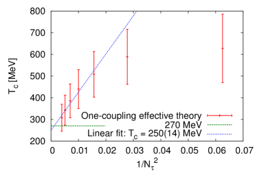
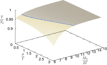
Figure 5: Left: Continuum extrapolation of critical temperature predicted by the effective theory. Right: Phase diagram for QCD with heavy quarks. From Fromm:2011qi .

4.2 Deconfinement transition in QCD with heavy quarks

Once quarks are included via the hopping expansion, a fully analytic evaluation becomes much more complex due to the additional couplings, but the effective theory can still be simulated efficiently. Moreover, while the partition function Eq. (25) still has a sign problem, it is considerably milder than that of 4d QCD, due to the fact that many degrees of freedom have been integrated out already. In Fromm:2011qi a flux representation of the effective theory including the static determinant was simulated, and the resulting phase diagram for $N_{f}=2,N_{\tau}=6$ is shown in Fig. 5 (right). Since the center symmetry of the Yang-Mills theory is explicitly broken by the quark determinant, the first-order transition weakens with decreasing quark mass until it vanishes at some critical value $m_{q}^{c}$. The transition also weakens with chemical potential, so that for $m_{q}>m_{q}^{c}$ one finds a first-order deconfinement transition coming from the $T$-axis and terminating in a critical endpoint, whose location depends on the quark mass. A continuum extrapolation would require larger $N_{\tau}$-values, which in turn demand higher orders for the hopping expansion to converge. Note that recent 4d QCD simulations using a hopping expanded determinant Ejiri:2019csa , as well as full QCD simulations Cuteri:2020yke permit control over the systematics at $\mu=0$.

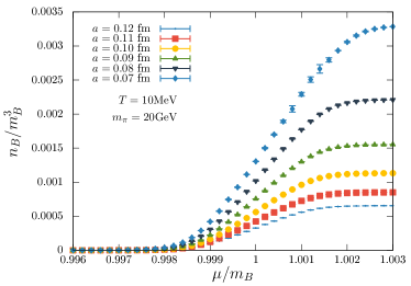
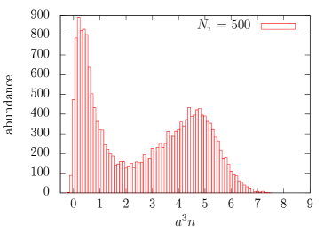
Figure 6: Left: Onset of baryon number (crossover) for heavy quarks and different lattice spacings Glesaaen:2015vtp . Right: First-order onset transition for light quarks and low $T$ (large $N_{\tau}$) Langelage:2014vpa .

4.3 Onset transition to baryon matter

With the same methods the cold and dense regime, where the sign problem is most severe, can also be studied. In particular, the onset transition to baryon matter has been seen explicitly to various orders in the combined expansions Fromm:2012eb ; Langelage:2014vpa ; Glesaaen:2015vtp . Once more valuable physical insight can be gained by an analytic calculation to leading order within the effective theory. In the strong coupling ($\beta=0$) limit with a static quark determinant only, the partition function factorises into one-site integrals which can be solved exactly. In the zero temperature limit, mesonic contributions are exponentially suppressed by chemical potential and for $N_{f}=1$ we have

$$Z(\beta=0)\stackrel{{\scriptstyle T\rightarrow 0}}{{\longrightarrow}}z_{0}^{V}\quad\mbox{with}\quad z_{0}=1+4h_{1}^{3}+h_{1}^{6},\quad h_{1}=(2\kappa e^{a\mu})^{N_{\tau}}=e^{(m-\mu)/T}\;.$$ (27)

This corresponds to a free baryon gas with two species. With one quark flavour only, there are no nucleons and the prefactor of the first term indicates a spin 3/2 quadruplet of $\Delta$’s, whereas the second term corresponds to a spin 0 six quark state or di-baryon. The quark number density is now easily evaluated

$$n=\frac{T}{V}\frac{\partial}{\partial\mu}\ln Z=\frac{1}{a^{3}}\frac{4N_{c}h_{1}^{N_{c}}+2N_{c}h_{1}^{2N_{c}}}{1+4h_{1}^{N_{c}}+h_{1}^{2N_{c}}}\;,\quad\lim_{T\rightarrow 0}a^{3}n=\left\{\begin{array}[]{cc}0,&\mu<m\\ 2N_{c},&\mu>m\end{array}\right.\;.$$ (28)

Thus at $T=0$ we find a discontinous transition when the quark chemical potential equals the constituent mass $m$. This reflects two expected physical phenomena: the “silver blaze” property of QCD, i.e. the fact that the baryon number stays zero for small $\mu$ even though the partition function explicitly depends on it Cohen:2003kd . Once the baryon chemical potential $\mu_{B}=3\mu$ is large enough to make a baryon ($m_{B}=3m$ in the static strong coupling limit), a discontinuous phase transition to a saturated baryon crystal takes place. The saturation density is $2N_{c}$ quarks per flavour and lattice site and reflects the Pauli principle. This is clearly a discretisation effect that has to disappear in the continuum limit.

In the case of two flavours the corresponding expression for the free gas of baryons reads

$$z_{0} = (1+4h_{d}^{3}+h_{d}^{6})+(6h_{d}^{2}+4h_{d}^{5})h_{u}+(6h_{d}+10h_{d}^{4})h_{u}^{2}+(4+20h_{d}^{3}+4h_{d}^{6})h_{u}^{3}$$ (29)

$$+(10h_{d}^{2}+6h_{d}^{5})h_{u}^{4}+(4h_{d}+6h_{d}^{4})h_{u}^{5}+(1+4h_{d}^{3}+h_{d}^{6})h_{u}^{6}\;,$$

with now two $h_{1}$ couplings for the $u$- and $d$-quarks. In this case we easily identify in addition the spin 1/2 nucleons as well has many other baryonic multi-quark states with their correct spin degeneracy. A similar result is obtained for mesons if we instead consider an isospin chemical potential in the low temperature limit Langelage:2014vpa . Remarkably, the entire spin-flavour-structure of the QCD bound states is obtained in this simple static strong coupling limit.

When corrections are added the step function is smoothed out. Fig. 6 (left) shows the baryon density computed through orders $O(\kappa^{8}u^{5})$ and plotted in continuum units. As the continuum is approached, the artefact of lattice saturation moves to infinity, as expected. Fig. 6 (left) shows a crossover, whereas for light quarks simulations show a first-order transition for large $N_{\tau}$, Fig. 6 (right), and a crossover for smaller $N_{\tau}$. This can again be understood with analytic insight from the hopping expansion. The dimensionless quantity

$$\epsilon(\mu,T)=\frac{e-n_{B}m_{B}}{n_{B}m_{B}}=-\frac{4}{3}\frac{1}{a^{3}n_{B}}\left(\frac{6h_{1}^{3}+3h_{1}^{6}}{z_{0}}\right)^{2}\,\kappa^{2}+\ldots\;,$$ (30)

here evaluated at $\beta=0$ in the simpler case $N_{f}=1$ Langelage:2014vpa , gives an interaction energy per baryon in units of the baryon mass when $T\rightarrow 0$. For $\mu<m$, it evaluates to zero in accordance with the silver blaze property. For $\mu>m$ it is nonzero and implies an attractive interaction, consistent with the baryon gas ‘condensing‘ to a liquid (or crystal on the lattice). Starting as $\sim\kappa^{2}$, it decreases with growing quark mass to zero in the static limit, as one would also expect from Yukawa potentials in nuclear physics. Hence, the end point of the liquid gas transition, $T_{c}(m)$, shrinks to zero with increasing quark mass, which explains the difference between the left and right of Fig. 6.

4.4 Large $N_{c}$ and quarkyonic matter

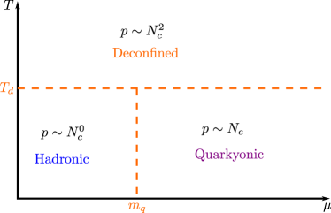
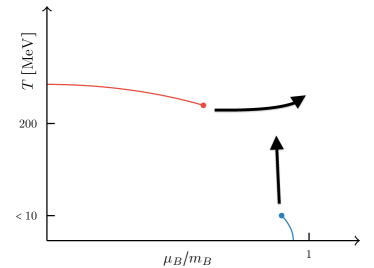
Figure 7: Left: Phase diagram for QCD with $N_{c}\rightarrow\infty$ McLerran:2007qj . Right: Evolution of the phase diagram for heavy quarks with growing $N_{c}$ Philipsen:2019qqm .

Interesting conjectures concerning the QCD phase structure were made some years ago, based on large $N_{c}$ arguments McLerran:2007qj . In particular, the phase diagram in the limit of large $N_{c}$, with fixed ’t Hooft coupling,

$$N_{c}\rightarrow\infty\quad\mbox{with}\quad\lambda_{H}=g^{2}N_{c}=\mathrm{const.},$$ (31)

was argued to look as in Fig. 7 (left). With fermion contributions suppressed by large $N_{c}$, the deconfinement transition is a straight line separating the plasma phase, where the pressure scales as $p\sim N_{c}^{2}$ (perturbation theory), from the hadron gas phase, where it scales as $p\sim N_{c}^{0}$ (ideal gas of hadrons). In McLerran:2007qj it is argued that at finite density there should then be a third phase with $p\sim N_{c}$, which was termed quarkyonic since it shows aspects of both baryon and quark matter. In particular, at low temperatures the fermi sphere in momentum space is argued to be composed of a baryonic shell of thickness $\sim\Lambda_{QCD}$, and quark matter inside.

With the analytic expansion tools and an effective lattice theory at hand, one can now adress these issues by direct calculations starting from QCD. For large $N_{c}$, the baryon mass grows as $m_{B}\sim N_{c}$, so the size of the constituent quark mass should not matter in that limit. This suggests to investigate the cold and dense region for large $N_{c}$ by direct calculation with the effective theory for heavy QCD. First, the effective theory of the previous sections was derived for a general number of colours Christensen:2013xea (see also Borisenko:2020prf ). Second, the onset transition to baryon matter has been analysed for general $N_{c}$ in Philipsen:2019qqm , where no large $N_{c}$ approximations are implied.

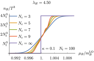
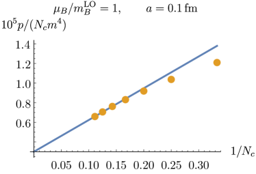
Figure 8: Left: The onset transition always becomes first order for large $N_{c}$.
Right: $p\sim N_{c}$ for large $N_{c}$ in baryon matter Philipsen:2019qqm .

Fig. 8 (left) shows the baryon onset transition to steepen with growing $N_{c}$, such that it always become first-order in the large $N_{c}$ limit when the t’Hooft coupling and $N_{\tau}$ are held fixed. This is independent of the value of $N_{\tau}$, which parametrises temperature. This strenghtening of the onset transition implies its critical endpoint $T_{c}(N_{c})$ to move to ever larger temperatures with growing $N_{c}$, as indicated in Fig. 7 (right). Together with the straightening of the deconfinement line with $N_{c}$, which follows from the behaviour of Feynman diagrams at large $N_{c}$, we thus understand how the conjectured phase diagram in Fig. 7 (left) emerges smoothly from the phase diagram with $N_{c}=3$ and heavy quarks. Furthermore, right after the onset transition $h_{1}\raise 1.29167pt\hbox{$>$\kern-7.5pt\raise-4.73611pt\hbox{$\sim$}}1$, through three orders in the hopping expansion at $\beta=0$, the coefficients of the pressure are proportional to $\sim N_{c}$ once $N_{c}$ is large, which is suggestive of a property to all orders. This $N_{c}$-scaling is stable under gauge corrections and, with a leading order correction in $N_{c}$, holds all the way down to $N_{c}=3-9$, Fig. 8 (right). Note also, that a lattice filling with baryon number smoothly changes from baryon matter (at the onset of condensation) to quark matter (at saturation) as a function of $\mu_{B}$, which is consistent with the momenum space picture of quarkyonic matter.

It thus seems that lattice QCD with heavy quarks shows the defining features ascribed to quarkyonic matter. On the other hand, for the moderate densities right after the baryon onset, one would expect no discernible difference from ordinary baryon matter. It remains an open question what happens at larger densities, in particular for the case of light quarks, when there may or may not be an additional chiral transition after baryon onset.

5 Effective lattice theory for chiral and light quarks

The light quark regime has also been addressed already a long time ago by effective theories at strong coupling. In particular, it was attempted to describe dense baryonic matter in Hamiltonian approaches, with constructions based on the strong coupling limit and partial chiral symmetry on the lattice Bringoltz:2002qc ; Bringoltz:2003jf ; Bringoltz:2006pz . Here, we stick to the Euclidean approach, starting from the partition function, to apply systematic expansions. However, being interested in the chiral phase transition, we now consder the lattice action with staggered fermions,

$$Z = \prod\limits_{x}\int d\chi_{x}d\bar{\chi}_{x}e^{2am_{q}\bar{\chi}_{x}\chi_{x}}\prod_{\ell}\int dU_{\ell}\;e^{-S_{\mathrm{YM}}[U]}\cdot e^{{\rm Tr}\left[U_{\ell}M_{\ell}^{{\dagger}}+U^{{\dagger}}_{\ell}M_{\ell}\right]},$$ (32)

$$\left(M^{{\dagger}}\right)_{i}^{j} = \eta_{\mu}(x)e^{a\mu_{B}\delta_{\mu,0}}\bar{\chi}_{x}^{i}\chi_{x+\mu,j},\qquad M_{k}^{l}=-\eta_{\mu}(x)e^{-a\mu_{B}\delta_{\mu,0}}\bar{\chi}_{x+\mu}^{k}\chi_{x,l},$$

where $(\ell,x,p)$ label lattice links, sites and plaquettes and $\eta_{\mu}(x)$ are the staggered phases. In the continuum limit, this represents $N_{f}=4$ QCD if no rooting is applied. Expanding in $\beta$, one obtains

$$Z = \prod\limits_{x}\int d\chi_{x}d\bar{\chi}_{x}\,\,e^{2am_{q}\bar{\chi}_{x}\chi_{x}}$$

$$\sum_{\{n_{p},\bar{n}_{p}\}}\!\prod_{\ell,p}\frac{\left(\frac{\beta}{2N_{c}}\right)^{n_{p}+\bar{n}_{p}}}{n_{p}!\bar{n}_{p}!}\!\!\int dU_{\ell}{\rm Tr}[U_{p}]^{n_{p}}{\rm Tr}[U^{{\dagger}}_{p}]^{\bar{n}_{p}}e^{{\rm Tr}\left[U_{\ell}M_{\ell}^{{\dagger}}+U^{{\dagger}}_{\ell}M_{\ell}\right]}\;,$$

with plaquette (anti-plaquette) occupation numbers $\{n_{p},\bar{n}_{p}\}$. In the strong coupling limit, $\beta=0$, the gauge action vanishes and the link integration reduces to one-link integrals Eriksson:1980rq . Subsequent integration over the Grassmann variables then yields the partition function as a sum over graphs in terms of mesons and baryons Rossi:1984cv . Leading $O(\beta)$-corrections have been derived in deForcrand:2014tha . Recently, after an intricate reorganisation of the involved degrees of freedom, an all-order dual formulation in terms of monomers, dimers, world lines and world sheets has been given Gagliardi:2017uag ; Gagliardi:2019cpa . Its contributions through $O(\beta^{2})$ can be simplified to

$$Z(m_{q},\mu) = \sum_{\{k,n,l,n_{p}\}}\underbrace{\prod_{b=(x,\nu)}\frac{(N_{c}-k_{b})!}{N_{c}!(k_{b}-|f_{b}|)!}}_{\tiny\mbox{meson hoppings}}\underbrace{\prod_{x}\frac{N_{c}!}{n_{x}!}(2am_{q})^{n_{x}}}_{\tiny\mbox{chiral condensate}}$$ (34)

$$\hskip 42.67912pt\times\underbrace{\prod_{l_{3}}w(l_{3},\mu)\prod_{l_{f}}\tilde{w}(l_{f},\mu)}_{\tiny\mbox{baryon hoppings}}\underbrace{\prod_{p}\frac{(\frac{\beta}{2N_{c}})^{n_{p}+\bar{n}_{p}}}{n_{p}!\bar{n}_{p}!}}_{\tiny\mbox{gluon propagation}}\;.$$

The integer valued occupation variables satisfy constraints at sites and bonds, which result from the Grassman and gauge integrations. Note that this formulation in general also contains negative weights, but the remaining sign problem is mostly mild enough to be handled by reweighting techniques. A particular advantage of this formulation is the feasibility to simulate the chiral limit directly, as well as any finite quark mass. On the other hand, gauge corrections are more difficult to include. Moreover, in the present formulation the expansion of the gauge sector in $\beta$ is slower to converge than the previously discussed character expansion, to which it might be extended in the future. Nevertheless, this formulation offers yet another road to studying QCD at finite density in a complementary parameter regime compared to the previous sections.

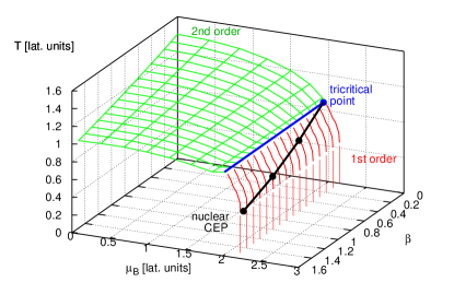
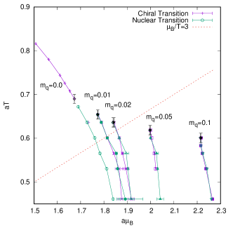
Figure 9: Left: Chiral phase transition and onset transition to baryon matter for $m=0$ deForcrand:2014tha .
Right: Mass dependence of the chiral and baryon onset transition at $\beta=0$ Kim:2016izx .

Early mean field Kawamoto:1981hw and Monte Carlo Karsch:1988zx studies based on a polymer representation have been restricted to the strong coupling limit, $\beta=0$. Modern simulations are done using a worm algorithm deForcrand:2009dh , which can be extended to include gauge corrections. Fig. 9 (left) shows the phase diagram in the chiral limit, $m=0$, both for $\beta=0$ and with leading gauge corrections $O(\beta)$ included deForcrand:2014tha . In the chiral limit there always is a non-analytic chiral phase transition, with a tricritical point where the first-order transition at finite density meets the second-order line. In the strong coupling limit, this tricritical point coincides with the end point of the nuclear liquid gas transition.

When gauge corrections are switched on, these start splitting up, but surprisingly the first-order lines of the chiral and nuclear transitions are still indistinguishably close. Fig. 9 (right) shows the strong coupling limit, but now with finite quark mass switched on. The second-order transition line changes to crossover, as expected. A very intersesting feature is the decrease with mass of the endpoint $T_{c}(m)$ of the nuclear liquid gas transition. Obtained from a different discretisation and in a very different parameter range, this behaviour agrees with the finding for heavy quarks discussed in the last sections. Note also that the endpoint of the chiral transition quickly moves to $\mu_{B}\raise 1.29167pt\hbox{$>$\kern-7.5pt\raise-4.73611pt\hbox{$\sim$}}3T$, which is consistent with all results reported for QCD at the physical point Ratti:2019tvj ; Philipsen:2019rjq .

6 Conclusions

In view of the sign problem of QCD at finite baryon density, which continues to evade purely algorithmic solutions, systematic studies of strong coupling methods, either directly or through development of effective theories, have provided a number of genuinely new results for QCD thermodynamics:

• The behaviour of screening masses for temperatures up to the crossover

• A derivation of the hadron resonance gas in the strong coupling regime

• The deconfinement transition for heavy quarks at all baryon chemical potentials

• The chiral phase transition in the massless limit in the region of strong, but finite, couplings

• The onset transition to baryon matter and its equation of state, both for heavy quarks on fine lattices and for light quarks on coarse lattices

• A smooth connection to thermodynamics at large $N_{c}$

These results were so far obtained in parameter regions away from the physical point in the continuum. Nevertheless, all the physics expected up to nuclear densities has been seen qualitatively on the lattice. It is now a matter of pushing these approaches to higher orders, and to evaluate them with refined algorithms. Given existing automatisation techniques to achieve high-order calculations for spin models and their sign problems, known in the condesed matter literature, the author believes this path is worth to be pursued further.

- (1) O. Philipsen, in Les Houches Summer School: Session 93: Modern perspectives in lattice QCD: Quantum field theory and high performance computing (2010)
- (2) G. Münster, Nucl. Phys. B 190, 439 (1981). DOI 10.1016/0550-3213(81)90570-8. [Addendum: Nucl.Phys.B 200, 536–538 (1982), Erratum: Nucl.Phys.B 205, 648–648 (1982)]
- (3) K. Seo, Nucl. Phys. B 209, 200 (1982). DOI 10.1016/0550-3213(82)90110-9
- (4) R. Balian, J.M. Drouffe, C. Itzykson, Phys. Rev. D 11, 2104 (1975). DOI 10.1103/PhysRevD.11.2104. [Erratum: Phys.Rev.D 19, 2514 (1979)]
- (5) J.M. Drouffe, J.B. Zuber, Phys. Rept. 102, 1 (1983). DOI 10.1016/0370-1573(83)90034-0
- (6) J. Polonyi, K. Szlachanyi, Phys. Lett. B 110, 395 (1982). DOI 10.1016/0370-2693(82)91280-1
- (7) F. Green, Phys. Lett. B 133, 99 (1983). DOI 10.1016/0370-2693(83)90114-4
- (8) F. Green, F. Karsch, Nucl. Phys. B 238, 297 (1984). DOI 10.1016/0550-3213(84)90452-8
- (9) A. Gocksch, M. Ogilvie, Phys. Lett. B 141, 407 (1984). DOI 10.1016/0370-2693(84)90273-9
- (10) F. Green, Nucl. Phys. B 215, 83 (1983). DOI 10.1016/0550-3213(83)90268-7
- (11) J. Langelage, G. Münster, O. Philipsen, JHEP 07, 036 (2008). DOI 10.1088/1126-6708/2008/07/036
- (12) C. Gattringer, Nucl. Phys. B 850, 242 (2011). DOI 10.1016/j.nuclphysb.2011.04.018
- (13) Y. Delgado Mercado, C. Gattringer, Nucl. Phys. B 862, 737 (2012). DOI 10.1016/j.nuclphysb.2012.05.009
- (14) F. Karsch, H.W. Wyld, Phys. Rev. Lett. 55, 2242 (1985). DOI 10.1103/PhysRevLett.55.2242
- (15) N. Bilic, H. Gausterer, S. Sanielevici, Phys. Rev. D 37, 3684 (1988). DOI 10.1103/PhysRevD.37.3684
- (16) G. Aarts, F.A. James, JHEP 01, 118 (2012). DOI 10.1007/JHEP01(2012)118
- (17) M. Wortis, in 12th School of Modern Physics on Phase Transitions and Critical Phenomena (1980)
- (18) J. Kim, A.Q. Pham, O. Philipsen, J. Scheunert, JHEP 10, 051 (2020). DOI 10.1007/JHEP10(2020)051
- (19) I. Montvay, G. Münster, Quantum fields on a lattice. Cambridge Monographs on Mathematical Physics (Cambridge University Press, 1997). DOI 10.1017/CBO9780511470783
- (20) J. Langelage, O. Philipsen, JHEP 01, 089 (2010). DOI 10.1007/JHEP01(2010)089
- (21) J. Langelage, O. Philipsen, JHEP 04, 055 (2010). DOI 10.1007/JHEP04(2010)055
- (22) J. Fingberg, U.M. Heller, F. Karsch, Nucl. Phys. B 392, 493 (1993). DOI 10.1016/0550-3213(93)90682-F
- (23) S. Datta, S. Gupta, Phys. Rev. D 67, 054503 (2003). DOI 10.1103/PhysRevD.67.054503
- (24) S. Borsanyi, G. Endrodi, Z. Fodor, A. Jakovac, S.D. Katz, S. Krieg, C. Ratti, K.K. Szabo, JHEP 11, 077 (2010). DOI 10.1007/JHEP11(2010)077
- (25) A. Bazavov, et al., Phys. Rev. D 90, 094503 (2014). DOI 10.1103/PhysRevD.90.094503
- (26) J. Kim, A.Q. Pham, O. Philipsen, J. Scheunert, PoS LATTICE2019, 065 (2019). DOI 10.22323/1.363.0065
- (27) B. Svetitsky, L.G. Yaffe, Nucl. Phys. B 210, 423 (1982). DOI 10.1016/0550-3213(82)90172-9
- (28) T.K. Herbst, M. Mitter, J.M. Pawlowski, B.J. Schaefer, R. Stiele, Phys. Lett. B 731, 248 (2014). DOI 10.1016/j.physletb.2014.02.045
- (29) A. Vuorinen, L.G. Yaffe, Phys. Rev. D 74, 025011 (2006). DOI 10.1103/PhysRevD.74.025011
- (30) C.S. Fischer, L. Fister, J. Luecker, J.M. Pawlowski, Phys. Lett. B 732, 273 (2014). DOI 10.1016/j.physletb.2014.03.057
- (31) C.S. Fischer, J. Luecker, J.M. Pawlowski, Phys. Rev. D 91(1), 014024 (2015). DOI 10.1103/PhysRevD.91.014024
- (32) P.M. Lo, B. Friman, K. Redlich, Phys. Rev. D 90(7), 074035 (2014). DOI 10.1103/PhysRevD.90.074035
- (33) C. Wozar, T. Kaestner, A. Wipf, T. Heinzl, Phys. Rev. D 76, 085004 (2007). DOI 10.1103/PhysRevD.76.085004
- (34) J. Greensite, K. Langfeld, Phys. Rev. D 87, 094501 (2013). DOI 10.1103/PhysRevD.87.094501
- (35) J. Greensite, K. Langfeld, Phys. Rev. D 88, 074503 (2013). DOI 10.1103/PhysRevD.88.074503
- (36) J. Greensite, K. Langfeld, Phys. Rev. D 90(1), 014507 (2014). DOI 10.1103/PhysRevD.90.014507
- (37) G. Bergner, J. Langelage, O. Philipsen, JHEP 11, 010 (2015). DOI 10.1007/JHEP11(2015)010
- (38) J. Langelage, S. Lottini, O. Philipsen, JHEP 02, 057 (2011). DOI 10.1007/JHEP07(2011)014. [Erratum: JHEP 07, 014 (2011)]
- (39) M. Fromm, J. Langelage, S. Lottini, O. Philipsen, JHEP 01, 042 (2012). DOI 10.1007/JHEP01(2012)042
- (40) O. Borisenko, V. Chelnokov, S. Voloshyn, Phys. Rev. D 102(1), 014502 (2020). DOI 10.1103/PhysRevD.102.014502
- (41) O. Borisenko, V. Chelnokov, E. Mendicelli, A. Papa, Nucl. Phys. B 965, 115332 (2021). DOI 10.1016/j.nuclphysb.2021.115332
- (42) J. Glesaaen, M. Neuman, O. Philipsen, JHEP 03, 100 (2016). DOI 10.1007/JHEP03(2016)100
- (43) J. Langelage, M. Neuman, O. Philipsen, JHEP 09, 131 (2014). DOI 10.1007/JHEP09(2014)131
- (44) S. Ejiri, S. Itagaki, R. Iwami, K. Kanaya, M. Kitazawa, A. Kiyohara, M. Shirogane, T. Umeda, Phys. Rev. D 101(5), 054505 (2020). DOI 10.1103/PhysRevD.101.054505
- (45) F. Cuteri, O. Philipsen, A. Schön, A. Sciarra, Phys. Rev. D 103(1), 014513 (2021). DOI 10.1103/PhysRevD.103.014513
- (46) M. Fromm, J. Langelage, S. Lottini, M. Neuman, O. Philipsen, Phys. Rev. Lett. 110(12), 122001 (2013). DOI 10.1103/PhysRevLett.110.122001
- (47) T.D.. Cohen, Phys. Rev. Lett. 91, 222001 (2003). DOI 10.1103/PhysRevLett.91.222001
- (48) L. McLerran, R.D. Pisarski, Nucl. Phys. A 796, 83 (2007). DOI 10.1016/j.nuclphysa.2007.08.013
- (49) O. Philipsen, J. Scheunert, JHEP 11, 022 (2019). DOI 10.1007/JHEP11(2019)022
- (50) A.S. Christensen, J.C. Myers, P.D. Pedersen, JHEP 02, 028 (2014). DOI 10.1007/JHEP02(2014)028
- (51) O. Borisenko, V. Chelnokov, S. Voloshyn, Nucl. Phys. B 960, 115177 (2020). DOI 10.1016/j.nuclphysb.2020.115177
- (52) B. Bringoltz, B. Svetitsky, Phys. Rev. D 68, 034501 (2003). DOI 10.1103/PhysRevD.68.034501
- (53) B. Bringoltz, B. Svetitsky, Phys. Rev. D 69, 014502 (2004). DOI 10.1103/PhysRevD.69.014502
- (54) B. Bringoltz, JHEP 03, 016 (2007). DOI 10.1088/1126-6708/2007/03/016
- (55) K.E. Eriksson, N. Svartholm, B.S. Skagerstam, J. Math. Phys. 22, 2276 (1981). DOI 10.1063/1.524760
- (56) P. Rossi, U. Wolff, Nucl. Phys. B 248, 105 (1984). DOI 10.1016/0550-3213(84)90589-3
- (57) P. de Forcrand, J. Langelage, O. Philipsen, W. Unger, Phys. Rev. Lett. 113(15), 152002 (2014). DOI 10.1103/PhysRevLett.113.152002
- (58) G. Gagliardi, J. Kim, W. Unger, EPJ Web Conf. 175, 07047 (2018). DOI 10.1051/epjconf/201817507047
- (59) G. Gagliardi, W. Unger, Phys. Rev. D 101(3), 034509 (2020). DOI 10.1103/PhysRevD.101.034509
- (60) J. Kim, W. Unger, PoS LATTICE2016, 035 (2016). DOI 10.22323/1.256.0035
- (61) N. Kawamoto, J. Smit, Nucl. Phys. B 192, 100 (1981). DOI 10.1016/0550-3213(81)90196-6
- (62) F. Karsch, K.H. Mütter, Nucl. Phys. B 313, 541 (1989). DOI 10.1016/0550-3213(89)90396-9
- (63) P. de Forcrand, M. Fromm, Phys. Rev. Lett. 104, 112005 (2010). DOI 10.1103/PhysRevLett.104.112005
- (64) C. Ratti, PoS LATTICE2018, 004 (2019). DOI 10.22323/1.334.0004
- (65) O. Philipsen, PoS LATTICE2019, 273 (2019). DOI 10.22323/1.363.0273