New physics explanations of $a_{\mu}$ in light of the FNAL muon $g-2$ measurement

Abstract

The Fermilab Muon $g-2$ experiment recently reported its first measurement of the anomalous magnetic moment $a_{\mu}^{\textrm{FNAL}}$, which is in full agreement with the previous BNL measurement and pushes the world average deviation $\Delta a_{\mu}^{\text{2021}}$ from the Standard Model to a significance of $4.2\sigma$. Here we provide an extensive survey of its impact on beyond the Standard Model physics. We use state-of-the-art calculations and a sophisticated set of tools to make predictions for $a_{\mu}$, dark matter and LHC searches in a wide range of simple models with up to three new fields, that represent some of the few ways that large $\Delta a_{\mu}$ can be explained. In addition for the particularly well motivated Minimal Supersymmetric Standard Model, we exhaustively cover the scenarios where large $\Delta a_{\mu}$ can be explained while simultaneously satisfying all relevant data from other experiments. Generally, the $a_{\mu}$ result can only be explained by rather small masses and/or large couplings and enhanced chirality flips, which can lead to conflicts with limits from LHC and dark matter experiments. Our results show that the new measurement excludes a large number of models and provides crucial constraints on others. Two-Higgs doublet and leptoquark models provide viable explanations of $a_{\mu}$ only in specific versions and in specific parameter ranges. Among all models with up to three fields, only models with chirality enhancements can accommodate $a_{\mu}$ and dark matter simultaneously. The MSSM can simultaneously explain $a_{\mu}$ and dark matter for Bino-like LSP in several coannihilation regions. Allowing under abundance of the dark matter relic density, the Higgsino- and particularly Wino-like LSP scenarios become promising explanations of the $a_{\mu}$ result.

^a Department of Physics and Institute of Theoretical Physics, Nanjing Normal University, Nanjing, Jiangsu 210023, China
^b School of Physics and Astronomy, Monash University, Melbourne, Victoria 3800, Australia
^c Institut für Kern- und Teilchenphysik, TU Dresden, Zellescher Weg 19, 01069 Dresden, Germany
E-mail: peter.athron@coepp.org.au, csaba.balazs@monash.edu, douglas.jacob@monash.edu,
wojciech.kotlarski@tu-dresden.de, dominik.stoeckinger@tu-dresden.de, hyejung.stoeckinger-kim@tu-dresden.de

1 Introduction

Precision measurements of the anomalous magnetic moment of the muon, $a_{\mu}$, provide excellent tests of physics beyond the Standard Model (BSM), and the results can give hints at what form it might take. Recently the E989 experiment [1] at the Fermi National Laboratory (FNAL) published the most precise measurement of the anomalous magnetic moment of the muon [2]. This result, and the previous result from Brookhaven National Laboratory (BNL) [3] (adjusted according to the latest value of $\mu_{\mu}/\mu_{p}$ as in Ref. [4]) and the new world average [2] are

$$a_{\mu}^{\textrm{FNAL}} ={\color[rgb]{0,0,0}(116\,592\,040\pm 54)\times 10^{-11}},$$ (1)

$$a_{\mu}^{\textrm{BNL}} =(116\,592\,089\pm 63)\times 10^{-11},$$ (2)

$$a_{\mu}^{\text{2021}} ={\color[rgb]{0,0,0}(116\,592\,061\pm 41)\times 10^{-11}}.$$ (3)

The FNAL measurement is fully compatible with the previous best measurement and has a smaller uncertainty. Compared to the BNL result, the new world average $a_{\mu}^{\text{2021}}$ has a slightly decreased central value and a 30% reduced statistics-dominated uncertainty. In parallel to the FNAL measurement, a worldwide theory initiative provided the White Paper [4] with the best estimate for the central theory prediction in the Standard Model (SM). Its value and uncertainty are

$$a_{\mu}^{\textrm{SM}} =(116\,591\,810\pm 43)\times 10^{-11}.$$ (4)

This SM prediction is based on up-to-date predictions of QED [5, 6], electroweak [7, 8], hadronic vacuum polarization [9, 10, 11, 12, 13, 14, 15] and hadronic light-by-light contributions [16, 17, 18, 19, 20, 21, 22, 23, 24, 25, 26, 27, 28, 29, 30]. For further discussion of recent progress we refer to Ref. [4]. The experimental measurements show the following deviations from the updated theoretical SM prediction:

$$\Delta a_{\mu}^{\textrm{FNAL}} ={\color[rgb]{0,0,0}(23.0\pm 6.9)\times 10^{-10}},$$ (5)

$$\Delta a_{\mu}^{\textrm{BNL}} =(27.9\pm 7.6)\times 10^{-10},$$ (6)

$$\Delta a_{\mu}^{\text{2021}} ={\color[rgb]{0,0,0}(25.1\pm 5.9)\times 10^{-10}}.$$ (7)

In each case the uncertainties are combined by summing them in quadrature. In the last line $\Delta a_{\mu}^{\text{2021}}$ is the new, updated deviation based on the experimental world average and the SM White Paper result. The long standing discrepancy between the BNL measurement and the SM theory prediction is confirmed and sharpened. Its significance is increased from $3.7\sigma$ to to $4.2\sigma$ by the combination with FNAL data.

This improvement has a significant impact on our understanding of BSM physics as it strengthens a major constraint on a variety of otherwise plausible SM extensions. In this paper we provide a comprehensive overview of this impact the FNAL measurement has on BSM physics. We examine the impact in minimal 1-, 2- and 3-field extensions of the SM, and in the well-motivated Minimal Supersymmetric Standard Model (MSSM). Within this theoretical framework we provide a thorough overview of the impact the FNAL measurement has and highlight promising scenarios that can explain it. In our investigation we use state-of-the-art $a_{\mu}$ calculations. For the simple SM extensions we use FlexibleSUSY [43, 44], which includes the universal leading logarithmic two-loop QED contributions in addition to the full one-loop calculation. For the MSSM we use GM2Calc [45], which implements a dedicated high-precision MSSM calculation including two-loop and higher-order contributions based on the on-shell scheme.

Reviews and general discussions of BSM contributions to $a_{\mu}$ have been given in Refs. [46, 25, 47, 48, 49, 50, 51]. Previously the deviation from BNL has been studied extensively in the literature. There was intensive activity proposing BSM explanations of the BNL result after its first discovery and in following years [52, 53, 54, 55, 56, 57, 58, 59, 60, 61, 62, 63, 64, 65, 66, 67, 68, 69, 70, 71, 72, 73, 74, 75, 76, 77, 78, 79, 80, 81, 82, 83, 84, 85, 86, 87, 88, 89, 90, 91, 92, 93, 94, 95, 96, 97, 98, 99, 100, 101, 102, 103, 104, 105, 106, 107, 108, 109, 110, 111, 112, 113, 114, 115, 116, 117, 118, 119, 120, 121, 122, 123, 124, 125, 126, 127, 128, 129, 130, 131, 132, 133, 134, 135, 136, 137, 138, 139, 140, 141, 142, 143, 144, 145, 146, 147, 148, 149, 150, 151, 152, 153, 154, 155, 156, 157, 158, 159, 160, 161, 162, 163]. Many ideas came under pressure from results at the LHC, and scenarios were proposed which could resolve tensions between $a_{\mu}$, LHC results and other constraints [164, 165, 166, 167, 168, 169, 170, 171, 172, 173, 174, 175, 176, 177, 178, 179, 180, 181, 182, 183, 184, 185, 186, 187, 188, 189, 190, 191, 192, 193, 194, 195, 196, 197, 198, 199, 200, 201, 202, 203, 204, 205, 206, 207, 208, 209, 210, 211, 212, 213, 214, 215, 216, 217, 218, 219, 220, 221, 222, 223, 224, 225, 226, 227, 228, 229, 230, 231, 232, 233, 234, 235, 236, 237, 238, 239, 240, 241, 242, 243, 244, 245, 246, 247, 248, 249, 250, 251, 252, 253, 254, 255, 256, 257, 258, 259, 260, 261, 262, 263, 264, 265, 266, 267, 268, 269, 270, 271, 272, 273, 274, 275, 276, 277, 278, 279, 280, 281, 282, 283, 284, 285, 286, 287, 288, 289, 290, 291, 292, 293, 294, 295, 296, 297, 298, 299, 300, 301, 302, 303, 304, 305, 306, 307, 308, 309, 310, 311, 312, 313, 314, 315, 316, 317, 318, 319, 320, 321, 322, 323, 324, 325, 326, 327, 328, 329, 330, 331, 332, 333, 334, 335, 336, 337, 338, 339, 340, 341, 342, 343, 344, 345, 346, 347, 348, 349, 350, 351, 352, 353, 354, 355, 356, 357, 358, 359, 360, 361, 362, 363, 364, 365, 366, 367, 368, 369, 370, 371, 372, 373, 374, 375, 376]. Many of these constructions use supersymmetry in some way and will be discussed in our Section 6, but this list also includes solutions motivated by extra dimensions [108, 109, 110, 111, 113, 238, 239, 112] and technicolor or compositeness [114, 115, 116, 117, 240, 118, 241, 119], or even introducing unparticle physics [150], as well as just extending models with new states like the two-Higgs doublet models [120, 121, 123, 122, 242, 244, 243, 246, 245, 247, 248, 249, 250, 251, 252, 253, 254, 256, 257, 255, 258, 259, 260, 261, 262, 263, 264] or adding leptoquarks [124, 125, 265, 266, 267, 268, 269, 270, 271, 272], new gauge bosons (including sub-GeV gauge bosons, dark photons and generalizations) [126, 127, 128, 131, 132, 133, 273, 288, 289, 290, 291, 279, 280, 276, 277, 129, 130, 275, 284, 281, 282, 283, 274, 292, 285, 286, 287, 278], Higgs triplets [156, 157] and vector-like leptons [289, 293, 294, 295, 296, 297, 298, 299, 300, 301, 302, 303, 304], or very light, neutral and weakly interacting scalar particles [305, 306, 307, 308, 309, 310, 311, 312, 313]. Some works have taken a systematic approach, classifying states according to representations and investigating a large set of them [367, 368, 369, 371, 370, 372, 373, 374, 375, 376, 152] .

The deviation found already by the BNL measurement also gave rise to the question whether it could be due to hypothetical, additional contributions to the hadronic vacuum polarization. If such additional effects would exist, they could indeed shift the SM prediction for $a_{\mu}$ towards the experimental value, but would at the same time worsen the fit for electroweak precision observables, disfavouring such an explanation of the deviation [411, 412, 413, 414, 415].

In spite of the vast number of works and the many varied ideas, for most models the same general principles apply. Typically the deviation requires new states with masses below the TeV scale or not much above $1$ TeV to explain the experimental value with perturbative couplings. The models which allow large $a_{\mu}$ with particularly large masses involve very large couplings and/or introduce enhancements through new sources of muon chirality flips (as we will describe in the next section). Therefore the absence of BSM signals at the LHC has led to tensions with large $a_{\mu}$ in many models: either very large couplings and heavy masses are needed or the stringent LHC limits have to be evaded in other ways.

Not only LHC, but also dark matter searches can lead to tensions in many models. The Planck experiment [416, 417] observed the dark matter abundance of the universe to be:

$$\Omega_{h^{2}}=0.1200\pm 0.001.$$ (8)

Since BSM contributions to $a_{\mu}$ are often mediated by new weakly interacting neutral particles, many interesting models also contain dark matter candidate particles. Any dark matter candidate particle with a relic density more than $0.12$ is over abundant and therefore strongly excluded. Further, the negative results of direct dark matter searches can lead to strong additional constraints on the model parameter spaces.

In the present work we aim to provide a comprehensive picture of the impact the new FNAL measurement has on BSM physics. The models we investigate in detail represent a wide range of possibilities. They cover models with new strongly or weakly interacting particles, with extra Higgs or SUSY particles, with or without a dark matter candidate, with or without new chirality flips and with strong or weak constraints from the LHC. In all cases we provide a detailed description of the mechanisms for the contributions to $a_{\mu}$; we then carry out detailed investigations of the model parameter spaces, including applicable constraints from the LHC and dark matter using state-of-the-art tools for evaluating constraints and LHC recasting. This allows us to answer which models and which model scenarios can accommodate the new FNAL measurement and the deviation $\Delta a_{\mu}^{\text{2021}}$ while satisfying all other constraints.

The rest of this paper is as follows. In Sec. 2 we explain how the anomalous magnetic moment appears in quantum field theories and emphasise the most important aspects which both make it an excellent probe of BSM physics and make the observed anomaly very difficult to explain simultaneously with current collider limits on new physics. In Secs. 3, 4, and 5 we present results for minimal 1-, 2- and 3-field extensions of the SM respectively that show the impact the new FNAL result has on these models. To provide a more global picture for 1- and 2-field extensions, in Sec. 3.1 and Sec. 4.1 we also classify models of this type systematically by quantum numbers and use known results to summarise their status with respect to explaining the BNL result, showing that this measurement severely restricts the set of possible models. This allows us to select models with the best prospects for detailed investigation, presenting results for the two-Higgs doublet model (Sec. 3.2), leptoquark models (Sec. 3.3) and two field extensions with scalar singlet dark matter (Sec. 4.2). For three field models we perform a detailed examination of models with mixed scalar singlet and doublet dark matter (Sec. 5.1) and fermion singlet and doublet dark matter (Sec. 5.2). In Sec. 6 we discuss the impact of the sharpened deviation on the MSSM, which is widely considered one of the best motivated extensions of the SM. This section also contains a brief self-contained discussion of $a_{\mu}$ and the possible enhancement mechanisms in the MSSM and explains in detail our treatment of dark matter data and LHC recasting. All constraints are then applied on the general MSSM, allowing all kinds of neutralino LSPs. Finally we present our conclusions in Section 7.

2 Muon $g-2$ and physics beyond the SM

In quantum field theory, the anomalous magnetic moment of the muon is given by

$$a_{\mu} =-2m_{\mu}F_{M}(0)\,,$$ (9)

where $m_{\mu}$ is the muon pole mass and $F_{M}(0)$ is the zero-momentum limit of the magnetic moment form factor. The latter is defined via the covariant decomposition of the 1-particle irreducible muon–muon–photon vertex function $\Gamma^{\mu}(p,-p^{\prime},q)$,

$$\bar{u}(p^{\prime})\Gamma^{\mu}(p,-p^{\prime},q)u(p) =-eQ\,\bar{u}(p^{\prime})\left[\gamma^{\mu}F_{V}(q^{2})+(p+p^{\prime})^{\mu}F_{M}(q^{2})+\ldots\right]u(p)$$ (10)

with the on-shell renormalized electric charge $e$, $Q=-1$, on-shell momenta $p^{2}=p^{\prime}{}^{2}=m_{\mu}^{2}$, on-shell spinors $u(p)$, $u(p^{\prime})$ and $q=p^{\prime}-p$. The quantum field theory operator corresponding to $a_{\mu}$ connects left- and right-handed muons, i.e. it involves a chirality flip.

The observable $a_{\mu}$ is CP-conserving, flavour conserving, loop induced, and chirality flipping. These properties make it complementary to many other precision and collider observables. In particular the need for a muon chirality flip has a pivotal influence on the BSM phenomenology of $a_{\mu}$. It requires two ingredients.

• Breaking of chiral symmetry. There must be a theory parameter breaking the chiral symmetry under which the left- and right-handed muon fields transform with opposite phases. In the SM and the MSSM and many other models this chiral symmetry is broken only by the non-vanishing muon Yukawa coupling $y_{\mu}$. In all these cases contributions to $F_{M}(0)$ are proportional to at least one power of the muon Yukawa coupling, where e.g. the MSSM Yukawa coupling is enhanced compared to the SM one.

  In some models, there are additional sources of breaking of the muon chiral symmetry. Examples are provided by the leptoquark model discussed below in Sec. 3.3, where the simultaneous presence of left- and right-handed couplings $\lambda_{L,R}$ and the charm- or top-Yukawa coupling breaks the muon chiral symmetry and leads to contributions governed by $\lambda_{L}\lambda_{R}m_{c,t}$. Similar mechanisms can also exist in the three-field models discussed below.

• Spontaneous breaking of electroweak gauge invariance. Since the $a_{\mu}$ operator connects a left-handed lepton doublet and right-handed lepton singlet it is not invariant under electroweak (EW) gauge transformations. Hence any contribution to $F_{M}(0)$ also must be proportional to at least one power of some vacuum expectation value (VEV) breaking EW gauge invariance. In the SM, there is only a single VEV $v$, so together with the required chirality flip, each SM-contribution to $F_{M}(0)$ must be proportional to $y_{\mu}v$ and thus to the tree-level muon mass. However, e.g. in the MSSM, there are two VEVs $v_{u,d}$; hence there are contributions to $a_{\mu}$ governed by $y_{\mu}v_{u}$, while the tree-level muon mass is given via $y_{\mu}v_{d}$. This leads to the well-known enhancement by $\tan\beta=v_{u}/v_{d}$.

In addition, the gauge invariant operators contributing to $a_{\mu}$ are (at least) of dimension six; hence any BSM contribution to $a_{\mu}$ is suppressed by (at least) two powers of a typical BSM mass scale. In conclusion, BSM contributions to $a_{\mu}$ can generically be parametrized as

$$\Delta a_{\mu}^{\text{BSM}} =C_{\text{BSM}}\frac{m_{\mu}^{2}}{M_{\text{BSM}}^{2}},$$ (11)

where $M_{\text{BSM}}$ is the relevant mass scale and where the coefficient $C_{\text{BSM}}$ depends on all model details like origins of chirality flips and electroweak VEVs as well as further BSM coupling strengths and loop factors.

An interesting side comment is that BSM particles will typically not only contribute to $a_{\mu}$ but also to the muon mass in similar loops, and those contributions depend on the same model details and scale as $\Delta m_{\mu}^{\text{BSM}}/m_{\mu}\sim{\cal O}(C_{\text{BSM}})$. The estimate $\Delta a_{\mu}^{\text{BSM}}\sim{\cal O}(\Delta m_{\mu}^{\text{BSM}}/m_{\mu})\times\frac{m_{\mu}^{2}}{M_{\text{BSM}}^{2}}$ is therefore valid in many models [53, 50]. One may impose a criterion that these BSM corrections to the muon mass do not introduce fine-tuning, i.e. do not exceed the actual muon mass. In models where this criterion is satisfied, $C_{\text{BSM}}$ can be at most of order unity and a generic upper limit,

$$\Delta a_{\mu}^{\text{BSM}}\lesssim{\cal O}(1)\frac{m_{\mu}^{2}}{M_{\text{BSM}}^{2}},$$ (12)

is obtained [53, 50]. In this wide class of models, imposing this criterion then implies an order-of-magnitude upper limit on the mass scale for which the value $\Delta a_{\mu}$ can be accommodated:

BNL: $$\Delta a_{\mu}^{\text{BSM}} ={\color[rgb]{0,0,0}27.9\times 10^{-10}} \Rightarrow\ M_{\text{BSM}} \lesssim{\cal O}(2)\text{TeV}$$ (13)

Including FNAL: $$\Delta a_{\mu}^{\text{BSM}} ={\color[rgb]{0,0,0}25.1\times 10^{-10}} \Rightarrow\ M_{\text{BSM}} \lesssim{\color[rgb]{0,0,0}{\cal O}(2.1)}\text{TeV}$$ (14)

In Appendix A we collect the generic one-loop Feynman diagrams which can contribute to $a_{\mu}$ in a general renormalizable quantum field theory. The results are expressed in terms of generic masses and couplings and reflect the above discussion. Contributions containing the factor $m_{\mu}^{2}$ correspond to chirality flips on the external muon line governed by the SM Yukawa coupling and VEV; the other contributions correspond to chirality flips via BSM couplings or fermion masses and require the simultaneous presence of BSM couplings to left- and right-handed muons, which in turn requires that some virtual states in the loop are not pure gauge eigenstates but mix via electroweak VEVs.

3 Single Field Extensions

In this section we discuss the impact of $a_{\mu}$ on simple single field extensions of the SM. Such extensions can be interesting in their own right or representative for more elaborate models with many new fields and particles and illustrate the impact of the $a_{\mu}$ measurement. We begin in Sec. 3.1 with a general overview of the status of one-field extensions, covering renormalizable models with new spin $0$, spin $1/2$ or spin $1$ fields. In Secs. 3.2-3.3 we then show the impact of the latest data on the two most interesting cases — the two-Higgs doublet model and leptoquark models.

3.1 Overview

Model	Spin	$SU(3)_{C}\times SU(2)_{L}\times U(1)_{Y}$	Result for $\Delta a_{\mu}^{\text{BNL}}$, $\Delta a_{\mu}^{\text{2021}}$
1	0	$({\bf 1},{\bf 1},1)$	Excluded: $\Delta a_{\mu}<0$
2	0	$({\bf 1},{\bf 1},2)$	Excluded: $\Delta a_{\mu}<0$
3	0	$({\bf 1},{\bf 2},-1/2)$	Updated in Sec. 3.2
4	0	$({\bf 1},{\bf 3},-1)$	Excluded: $\Delta a_{\mu}<0$
5	0	$({\bf\overline{3}},{\bf 1},1/3)$	Updated Sec. 3.3.
6	0	$({\bf\overline{3}},{\bf 1},4/3)$	Excluded: LHC searches
7	0	$({\bf\overline{3}},{\bf 3},1/3)$	Excluded: LHC searches
8	0	$({\bf 3},{\bf 2},7/6)$	Updated Sec. 3.3.
9	0	$({\bf 3},{\bf 2},1/6)$	Excluded: LHC searches
10	$1/2$	$({\bf 1},{\bf 1},0)$	Excluded: $\Delta a_{\mu}<0$
11	$1/2$	$({\bf 1},{\bf 1},-1)$	Excluded: $\Delta a_{\mu}$ too small
12	$1/2$	$({\bf 1},{\bf 2},-1/2)$	Excluded: LEP lepton mixing
13	$1/2$	$({\bf 1},{\bf 2},-3/2)$	Excluded: $\Delta a_{\mu}<0$
14	$1/2$	$({\bf 1},{\bf 3},0)$	Excluded: $\Delta a_{\mu}<0$
15	$1/2$	$({\bf 1},{\bf 3},-1)$	Excluded: $\Delta a_{\mu}<0$
16	$1$	$({\bf 1},{\bf 1},0)$	Special cases viable
17	$1$	$({\bf 1},{\bf 2},-3/2)$	UV completion problems
18	$1$	$({\bf 1},{\bf 3},0)$	Excluded: LHC searches
19	$1$	$({\bf\overline{3}},{\bf 1},-2/3)$	UV completion problems
20	$1$	$({\bf\overline{3}},{\bf 1},-5/3)$	Excluded: LHC searches
21	$1$	$({\bf\overline{3}},{\bf 2},-5/6)$	UV completion problems
22	$1$	$({\bf\overline{3}},{\bf 2},1/6)$	Excluded: $\Delta a_{\mu}<0$
23	$1$	$({\bf\overline{3}},{\bf 3},-2/3)$	Excluded: proton decay

Table 1: Summary of known results for gauge invariant single field extensions with one-loop contributions to the anomalous magnetic moment of the muon. These results are rather exhaustive due to systematic investigations and classifications in Ref. [367, 369, 371, 370]. Note however that while we present the results based on representations of SM gauge and Lorentz symmetries, the references make assumptions that can be important to the conclusions and are different in each paper. Thus the conclusions summarised in this table should be interpreted with care. For more information on models 1-2, 3-4, 5-9, 10-12, 13, 14-18 and 19-23 see references [419, 371, 420, 421], [367, 371], [124, 371], [152, 367, 371], [371], [152, 367, 371, 370, 422] and [370], respectively. We use color highlighting to give a visual indication of the status of the model, namely green for viable explanations, red for excluded and purple for vector extensions excluded on the basis of their UV completions.

Before presenting our updated results for those cases in Secs. 3.2-3.3, we first classify the single field extensions according to their spin and their SM representations and charges, and discuss the known results to provide a very important overview of what is possible and put our new results in the appropriate context. Single field models have been classified or reviewed in a systematic manner in Refs. [367, 369, 421, 371, 370], with the results summarized in Table 1.

The confirmation of a large positive deviation from the SM prediction in the anomalous magnetic moment of the muon rules out most one-field extensions of the SM. The reasons for this are simple. First to explain the anomaly these models must provide a positive contribution to $a_{\mu}$, and this constraint alone rules out a large number of the possible extensions. Secondly even if the sign of the contribution is positive, the models must have a chirality flip in order for the contribution to be large enough with perturbative couplings. Without a chirality flipping enhancement, contributions that explain $a_{\mu}$ require the masses of the new particles to be so light that they would already have been observed in collider experiments.

Ref. [367] considers scalars, fermions and vectors. For fermions and scalars they considered gauge invariant extensions with $SU(3)$ singlets, which may be $SU(2)$ singlets, doublets, triplets ($Y=-1$) and adjoint triplets ($Y=0$) for fermions, and doublets and triplets for scalars. They do not consider scalars obtaining a VEV. They treated vector states as simplified models of neutral and charged vector states without specifying any gauge extension. They assume minimal flavour violating interactions with leptons (see 2.2 of Ref. [367] for details) for LEP contact interaction limits and LHC searches, and perform the calculation of $\Delta a_{\mu}$ at the one-loop level. They obtained a negative contribution to $a_{\mu}$ from the scalar triplet, the neutral fermion singlet, and fermion triplets with hypercharge $0$ or $-1$, and found that while a charged fermion singlet can give a positive contribution it is always too small to explain $\Delta a_{\mu}^{\textrm{BNL}}$. They found scalar and fermion doublet scenarios that could accommodate $\Delta a_{\mu}^{\textrm{BNL}}$ at the $1\sigma$ level were ruled out by LEP searches for neutral scalars and LEP limits on mixing with SM leptons respectively. For a single neutral vector boson, they find that the region where $\Delta a_{\mu}^{\textrm{BNL}}$ can be explained within $1\sigma$ is entirely ruled out by LEP constraints from 4-fermion contact interactions and resonance searches. They also consider a single charged vector boson coupling to a right handed charged lepton and a right handed neutrino, and find that in this case the region where $\Delta a_{\mu}^{\textrm{BNL}}$ can be explained within $1\sigma$ is ruled out by the combination of LEP limits on contact interactions and LHC direct searches. In summary they find that all gauge invariant one-field extensions they considered failed to explain the anomaly. This paper’s findings are reflected in Table 1, except for the cases of the scalar doublet (see Sec.3.2) and the neutral vector (see the discussion in Sec. 3.1.1 at the end of this overview), where there is a lot of dedicated literature and it is known that breaking the assumptions of Ref. [367] can change the result.

Refs. [421, 371, 369] also take a systematic approach. Ref. [421] considers scalar bosons. Compared to results in the other papers this adds the singly charged $SU(2)$ singlets to Table 1. This result was also used in the classification in Ref. [371] (drawing also from Ref. [419]), along with doubly charged $SU(2)$ scalar singlets using results from Ref. [420] and scalar leptoquarks (see Sec. 3.3 for our update) originally proposed in Ref. [124]. They also add a new result for a fermion $SU(2)$ singlet with hypercharge $-3/2$, i.e. the fermion state $({\bf 1},{\bf 2},-3/2)$, showing that the contribution is always negative above the LEP limit. Otherwise their classification overlaps with Ref. [367] and the conclusions are effectively consistent. Ref. [369] does not require $SU(2)_{L}$ invariance and instead considers simplified models of Lorentz scalar, fermion and vector states with results presented in terms of axial and vector couplings, $g_{a}$ and $g_{v}$ and classify states according to electromagnetic charges and $SU(3)$ representations. The reference presents plots of $\Delta a_{\mu}$ predictions against the mass of the new state for specific cases of the couplings. We checked that the results are consistent with what we present in Table 1, but Ref. [369] does not contain additional general conclusions on the viability of each case.

While Refs. [367] and [369] used a simplified models treatment of vector states, Ref. [370] systematically classified vector extensions according to SM gauge representations and considered the implications of embedding these into a UV complete gauge extension of the SM. They found that only $({\bf 1},{\bf 1},0)$ may provide a viable UV complete explanation of $\Delta a_{\mu}^{\textrm{BNL}}$, depending on specific model dependent details (see Sec. 3.1.1 below for more details on such explanations). Although the $({\bf 1},{\bf 2},-3/2)$ vector state gives large contributions to $a_{\mu}$, they rejected this since the UV completion into 331 models cannot provide a $\Delta a_{\mu}^{\textrm{BNL}}$ explanation consistent with experimental limits [422]. A $({\bf 1},{\bf 3},0)$ vector state has no chirality flip, so explanations are ruled out by LHC limits [423]. $({\bf\overline{3}},{\bf 1},-2/3)$ and $({\bf\overline{3}},{\bf 2},-5/6)$ have chirality flipping enhancements, but they reject $({\bf\overline{3}},{\bf 1},-2/3)$ based on an $SU(4)_{C}\times SU(2)_{L}\times U(1)_{R}$ UV completion and limits on the masses from rare decays [424], while the $({\bf\overline{3}},{\bf 2},-5/6)$ state is rejected based on an $SU(5)$ UV completion and proton decay limits. Models without chirality flip enhancements ($({\bf\overline{3}},{\bf 1},-5/3)$, $({\bf\overline{3}},{\bf 2},1/6)$ and $({\bf\overline{3}},{\bf 3},-2/3)$) can all be ruled out by collider constraints or because they give the wrong sign. A summary of the constraints excluding each of the vector leptoquarks are included in Table 1.

3.1.1 Dark photon and dark $Z$ explanations

Before concluding this overview we now briefly discuss the particularly interesting case of an additional gauge field $Z_{d}$ with $({\bf 1},{\bf 1},{\bf 0})$ quantum numbers that arises from some additional $U(1)_{d}$ gauge symmetry. The dark photon scenario assumes that the known quarks and leptons have no $U(1)_{d}$ charge. The potential impact of dark photons on $a_{\mu}$ has been extensively studied, after the first proposal in Ref. [132]. Models with a general Higgs sector contain both kinetic mixing of the SM $B$-field and $Z_{d}$ and the mass mixing of the SM $Z$-field and $Z_{d}$. As the mass mixing parameter is typically far smaller than the kinetic mixing one, the leading contribution to $a_{\mu}$ is proportional to the kinetic mixing parameter $\epsilon$. The kinetic mixing term induces an interaction between the SM fermions and the dark photon, and the region relevant for significant $\Delta a_{\mu}$ has first been found to be $10^{-6}<\epsilon^{2}<10^{-4}$, with dark photon masses in the range between $1\text{ MeV}\cdots 500\text{ MeV}$ [132]. However the electron anomalous magnetic moment result [425] reduces the mass range to $20\text{ MeV}\cdots 500\text{ MeV}$ [289], and the remaining range is excluded by the following experimental results obtained from various dark photon production channels from A1 in Mainz [426] (radiative dark photon production in fixed-target electron scattering with decays into $e^{+}e^{-}$ pairs), BaBar [427] (pair production in $e^{+}e^{-}$ collision with subsequent decay into $e^{+}e^{-}$ or $\mu^{+}\mu^{-}$ pairs), NA48/2 at CERN [428] ($\pi^{0}$ decay modes via dark photon and subsequent decay into $e^{+}e^{-}$-pair) and from dark matter production via dark photon from NA46 at the CERN [429].

As a result, pure dark photon models cannot accommodate significant contributions to $a_{\mu}$. Extensions, e.g. so-called “dark $Z$” models, open up new possibilities but are also strongly constrained [288, 289, 290, 305, 292]. Similarly, neutral $Z^{\prime}$ vector bosons with direct gauge couplings to leptons are also strongly constrained (as indicated in Tab. 1); for examples of remaining viable possibilities with significant contributions to $a_{\mu}$ we mention the model with gauged $L_{\mu}-L_{\tau}$ quantum number and generalizations thereof, see Refs. [273, 274, 277, 283, 430, 285, 278]. Even in such viable models only rather small parts of the parameter space are promising; in particular only specific windows for the new vector boson masses can lead to viable explanations of $\Delta a_{\mu}^{\text{2021}}$. In case of the $L_{\mu}-L_{\tau}$ model, the recent Ref. [393] has shown that essentially only the mass range between $0.01\ldots 0.1$GeV remains, and that this parameter range can be further probed in the future by muon fixed-target experiments and even by neutrino and dark matter search experiments. For very heavy $Z^{\prime}$ masses in the TeV region, explanations of $\Delta a_{\mu}^{\text{2021}}$ are already disfavoured by LHC data, but further constraints can ultimately be obtained at a muon collider [278]. In case of “dark $Z$” models, the viable mass range is below the 1 GeV scale, and the promising parameter space can be probed by measurements of the running weak mixing angle at low energies at facilities such as JLab QWeak, JLab Moller, Mesa P2, see e.g. Refs. [290, 383].

3.2 Two-Higgs Doublet Model

As can be seen in Table 1, the two-Higgs doublet model is one of the very few viable one-field explanations of $\Delta a_{\mu}^{\textrm{BNL}}$. It is in fact the only possibility without introducing new vector bosons or leptoquarks. The two-Higgs doublet model (2HDM) contains a charged Higgs $H^{\pm}$, a CP-odd Higgs $A$, and two CP-even Higgs bosons $H,h$, where $h$ is assumed to be SM-like (we assume here a CP-conserving Higgs potential, which is sufficient to maximize contributions to $a_{\mu}$). To be specific we list here the Yukawa Lagrangian for the neutral Higgs bosons in a form appropriate for the 2HDM of type I, II, X, Y and the flavour-aligned 2HDM, in the form of Ref. [251],

$${\cal{L}}_{Y}= -\sum_{{\cal S}=h,H,A}\sum_{f}\,\frac{Y_{f}^{\cal S}m_{f}}{v}\,{\cal S}{\bar{f}}P_{\text{R}}f+h.c.,$$ (15)

$$Y^{h}_{f}= \sin(\beta-\alpha)+\cos(\beta-\alpha)\zeta_{f}, Y^{A}_{d,l}= -\zeta_{d,l}\,,$$ (16)

$$Y^{H}_{f}= \cos(\beta-\alpha)-\sin(\beta-\alpha)\zeta_{f}, Y^{A}_{u}= +\zeta_{u}\,.$$ (17)

where the Dirac fermions $f$ run over all quarks and leptons, $(\beta-\alpha)$ is a mixing angle and $\sin(\beta-\alpha)=1$ corresponds to $h$ being SM-like. The dimensionless Yukawa prefactors $\zeta_{f}$ depend on the 2HDM version and will be specialized later.

The 2HDM has a rich phenomenology with a plethora of new contributions to the Higgs potential and the Yukawa sector. It differs from the previously mentioned models in that two-loop contributions to $a_{\mu}$ are known to be crucial. Typically the dominant contributions arise via so-called Barr-Zee two-loop diagrams. In these diagrams an inner fermion loop generates an effective Higgs–$\gamma$–$\gamma$ interaction which then couples to the muon via a second loop. If the new Higgs has a large Yukawa coupling to the muon and if the couplings in the inner loop are large and the new Higgs is light, the contributions to $a_{\mu}$ can be sizeable. The Higgs mediated flavour changing neutral currents in the 2HDM can be avoided by imposing either $\mathbb{Z}_{2}$ symmetry or flavour-alignment.

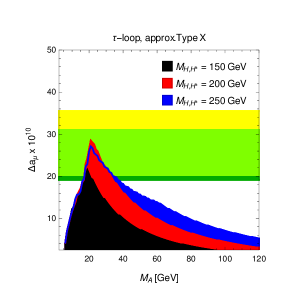
(a)

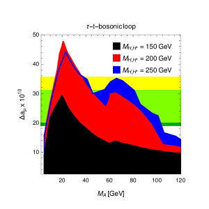
(b)

Figure 1: The maximum results for $\Delta a_{\mu}$ in the two versions of the two-Higgs Doublet Model with minimal flavour violation, compared with the $1\sigma$ regions around $\Delta a_{\mu}^{\textrm{BNL}}$ (yellow) and new world average $\Delta a_{\mu}^{\text{2021}}$ (green); light green shows the overlap between the two regions. The maximum results are shown as functions of $M_{A}$, for three different values of $M_{H,H^{\pm}}$, as indicated: (a) lepton-specific/type X model (b) flavour-aligned two-Higgs Doublet Model. The results are based on Ref. [252]. The left plot is technically obtained in the framework of the flavour-aligned model but taking only $\tau$-loop contributions, which coincides with the type X model.

Fig. 1 presents up-to-date results of the possible contributions $\Delta a_{\mu}$ in both of these versions of the 2HDM. The figure is based on results of Ref. [252] and compares them to the new world average $\Delta a_{\mu}^{\text{2021}}$ obtained from including the FNAL value. It arises from scans of the model parameter space and shows the maximum possible $\Delta a_{\mu}$ as a function of the most important parameters, the two new Higgs masses $M_{A}$ and $M_{H}$, where the choice $M_{H}=M_{H^{\pm}}$ maximises $\Delta a_{\mu}$. The reason why there are absolute upper limits on $\Delta a_{\mu}$ is a combination of theoretical and experimental constraints, as discussed in the following.

Fig. 1(a) shows the results for the 2HDM type X, the so-called lepton-specific version of the 2HDM with $\mathbb{Z}_{2}$ symmetry. A general analysis of all types of the 2HDM with discrete $\mathbb{Z}_{2}$ symmetries and minimal flavour violation has been done in Ref. [242], where only this lepton-specific type X model survived as a possible source of significant $\Delta a_{\mu}$. In this model, the parameters of Eq. (15) are $\zeta_{l}=-\tan\beta$ for all charged leptons, while $\zeta_{u,d}=\cot\beta$ for all quarks. The $\tan\beta$-suppression of quark Yukawa couplings helps evading experimental constraints from LEP, LHC and flavour physics. In the type X 2HDM the main contributions arise from Barr-Zee diagrams with an inner $\tau$-loop, which are $(\tan\beta)^{2}$-enhanced. Hence important constraints arise from e.g. precision data on $Z\to\tau\tau$ and $\tau$-decay [244, 246, 249, 253] as well as from LEP data on the mass range $M_{A}\lesssim 20$ GeV [252]. As Fig. 1(a) shows, only a tiny parameter space in the 2HDM type X remains a viable explanation of the observed $\Delta a_{\mu}^{\text{2021}}$. For a $1\sigma$ explanation, $M_{A}$ must be in the small interval $20\ldots 40$ GeV; the corresponding maximum values of the $\tan\beta$ parameter, which governs the lepton Yukawa couplings in this model, are in the range $50\ldots 100$. The masses of the new heavier Higgs bosons $M_{H,H^{\pm}}$ vary between $150$ and $250$ GeV in the figure. Smaller values of these masses lead to stronger constraints (since loop contributions to $\tau$-physics are less suppressed), while larger values lead to a larger hierarchy $M_{A}\ll M_{H,H^{\pm}}$ which leads to stronger constraints from electroweak precision physics and theoretical constraints such as perturbativity [249, 252]. We mention also that the 2HDM type X parameter space with particularly large contributions to $a_{\mu}$ can lead to peculiar $\tau$-rich final states at LHC [247, 256] but can be tested particularly well at a future lepton collider [431] and is also compatible with CP violation and testable contributions to the electron electric dipole moment [255].

Fig. 1(b) shows results for the so-called flavour-aligned two-Higgs doublet model, which is a more general but still minimal flavour violating scenario. Here the parameters $\zeta_{l}$, $\zeta_{u}$, $\zeta_{d}$ are independent, however assumed to be generation-universal. The contributions to $a_{\mu}$ were first discussed in Ref. [245] and then scrutinized in Refs. [243, 251, 252]. Here not only the $\tau$-lepton loop contributes in essentially the same way as before, but also Barr-Zee diagrams with the top-quark in the inner loop may contribute. To a smaller extent, also purely bosonic two-loop diagrams can increase $a_{\mu}$. The plot takes into account all contributions, based on Refs. [251, 252]. In particular the top-quark loop leads to a larger possible value of $a_{\mu}$. Its contributions are bounded by constraints from LHC data and $B$-physics. The LHC constraints are weaker for $M_{A}>62$ GeV, where the decay $h\to AA$ is kinematically impossible [252]. This is reflected in the behaviour of the maximum $\Delta a_{\mu}$ as a function of $M_{A}$ in the plot. In case of the flavour-aligned 2HDM the world average deviation $\Delta a_{\mu}^{\text{2021}}$ can be accommodated for $M_{A}$ up to $100$ GeV, if the heavy and charged Higgs masses are in the region $M_{H}=M_{H^{\pm}}=200\ldots 250$ GeV. In the parameter space which maximises $\Delta a_{\mu}$ in the flavour-aligned 2HDM the light $A$-boson has simultaneously significant Yukawa couplings to the top quark and to $\tau$-leptons, leading to a significant rate for the process $gg\to A\to\tau\tau$, which might be tested at future LHC runs.

Hence among the 2HDM versions without tree-level FCNC, the well-known type I and type II versions are excluded as explanations of the deviation $\Delta a_{\mu}^{\text{2021}}$. In contrast, the lepton-specific type X model and the more general flavour-aligned 2HDM can give significant contributions to $\Delta a_{\mu}$. In both cases, two-loop Barr-Zee diagrams with $A$-boson exchange and $\tau$-loop are important; in the flavour-aligned model also top-loops are important. The mass $M_{A}$ is severely constrained and the new Yukawa couplings must be at their upper experimental limits. Because of this, the 2HDM explanations of $\Delta a_{\mu}^{\text{2021}}$ are going to be further scrutinized at ongoing and future experiments: Any improvement of the LHC sensitivity to $gg\to A\to\tau\tau$ can either discover the $A$-boson or reduce the allowed parameter space visible in Fig. 1(b). Likewise, improved measurements of $\tau$-decays can lead to reduced upper limits on the maximum $\tan\beta$ or $\zeta_{l}$, respectively, and reduce the viable parameter space in both plots. As mentioned above, Refs. [247, 256] have investigated how further future LHC measurements of processes such as $HA$ or $H^{\pm}A$ production with decay into multi-lepton final states can impact the 2HDM explanations of $\Delta a_{\mu}^{\text{2021}}$. Lepton colliders even with modest c.o.m. energy offer additional coverage of the 2HDM parameter space via the Yukawa process $e^{+}e^{-}\to\gamma^{*}/Z^{*}\to\tau\tau A$ [431], which is directly sensitive to the low-mass pseudoscalar Higgs boson relevant for $a_{\mu}$.

Further, we mention that more exotic variants of the 2HDM which involve neither $\mathbb{Z}_{2}$-symmetric nor general flavour-aligned Yukawa couplings can open up additional possibilities. E.g. large non-flavour aligned Yukawa couplings to $\tau$-leptons or top quarks can allow large contributions to $a_{\mu}$ even for masses of $M_{A}$ above $100$ GeV [256, 331]. In these cases, important constraints arise from lepton flavour violating processes [256] and B-physics [331]. Large, non-flavour aligned $\tau$-Yukawa couplings also allow another window of significant contributions with a very light CP-even Higgs with $M_{H}\lesssim 1$ GeV [259]. And a muon-specific 2HDM can accommodate large $\Delta a_{\mu}$ with $\tan\beta$ of order $1000$ [250].

3.3 Scalar Leptoquarks

In this subsection we update the results for the other single field models which could explain $\Delta a_{\mu}^{\textrm{BNL}}$, i.e. the scalar leptoquarks. Scalar and vector leptoquarks that interact with SM leptons and quarks can appear as the only BSM particle in one-loop contributions to the anomalous magnetic moment of the muon. Scalar leptoquarks have been considered as a solution for the anomalous magnetic moment anomaly in Refs. [124, 369, 371, 432, 433], while vector leptoquarks have also been considered in Refs. [369, 370]. Here we focus on studying scalar leptoquarks in detail, since one would expect vector leptoquarks to be associated with an extension of the gauge symmetries, which complicates the construction of these models, and taking the simplified model approach they may yield results which are rather misleading compared to what can be achieved in a realistic model.

Requiring gauge invariant couplings to SM leptons and quarks restricts us to the five scalar leptoquarks [434] shown in Table 1 (Models 5–9). Only two of these models, $S_{1}$ $({\bf\overline{3}},{\bf 1},1/3)$ and $R_{2}$ $({\bf 3},{\bf 2},7/6)$, have both left- and right-handed couplings to the SM fermions and can therefore have a chirality flip enhancing their one-loop contributions [124, 369, 371].

Leptoquarks can in general have complicated flavour structure in their couplings. Since our focus is on demonstrating the impact of the anomalous magnetic moment experiment and demonstrating the various ways to explain it, we prefer to simplify the flavour structure and focus on the couplings that lead to an enhanced $\Delta a_{\mu}$ contribution. We therefore restrict ourselves to muon-philic leptoquarks that couple only to the second-generation of SM leptons, evading constraints on flavour violating processes such as $\mu\rightarrow e\gamma$. Leptoquarks that induce flavour violation in the quark sector have been widely considered in the literature as possible solutions to flavour anomalies, and sometimes simultaneous explanations of $a_{\mu}$ and these anomalies (see e.g. Refs. [432, 433]). However we also do not consider these here for the same reasons we choose to avoid lepton flavour violating couplings and the same reasoning applies to simultaneous explanations of the more recent $a_{e}$ anomaly [435].

We found that it is possible to explain the $\Delta a_{\mu}^{\textrm{BNL}}$ and $\Delta a_{\mu}^{\text{2021}}$ results with moderately sized perturbative couplings using leptoquarks that are both muon-philic and charm-philic, i.e. leptoquarks that only couple to second generation up-type quarks as well as only second generation charged leptons. Specifically we found $\Delta a_{\mu}^{\textrm{BNL}}$ could be explained while satisfying LHC limits from direct searches as long as $\sqrt{|\lambda_{L}\lambda_{R}|}\gtrsim 0.4$, where $\lambda_{L}$ and $\lambda_{R}$ are the leptoquark couplings to the muons and the quarks. However careful consideration of CKM mixing and flavour changing neutral currents (FCNC) reveals stringent constraints. While one may require that the new states couple only to the charm and not the up-quark or top-quark, CKM effects will then still generate couplings to the bottom and down-quark. This effect is very important and the impact of these for “charm-philic” leptoquark explanations of $\Delta a_{\mu}^{\textrm{BNL}}$ has been considered in Ref. [267]. There they find that constraints from BR($K^{+}\rightarrow\pi^{+}\nu\overline{\nu}$) for the $S_{1}$ leptoquark, or BR($K_{L}\rightarrow\mu^{+}\mu^{-}$) for the $R_{2}$ leptoquark, heavily restrict one of the couplings that enter the $a_{\mu}$ calculation. They find this excludes fitting $\Delta a_{\mu}^{\textrm{BNL}}$ within $1\sigma$, but in the case of the first model an explanation within $2\sigma$ remained possible, while for the second model explanations well beyond $2\sigma$ were excluded. They also consider the possibility that it is the down-type couplings that are second generation only, and find even more severe constraints in that case. Finally for a limited case, they explore including a direct coupling to the top-quark and find that quite large couplings to the top quark are needed to explain $\Delta a_{\mu}^{\textrm{BNL}}$ within $1\sigma$. Due to the strong flavour constraints from coupling the leptoquark to the second generation of SM quarks, we instead present results for top-philic leptoquarks, i.e. using scalar leptoquarks which couple to the second generation SM leptons, and the third generation of SM quarks.

Below is written the Lagrangian for both scalar leptoquarks, where here all fermions are written as 2-component left-handed Weyl spinors, for example $Q_{3}=(t_{L},b_{L})^{T}$ and $\mu_{R}^{\dagger}$, which follows the notation of Ref. [436]. For simplicity we also define $\mu,t,b:=\mu_{R}^{\dagger},t_{R}^{\dagger},b_{R}^{\dagger}$ below.

$${\cal L}_{S_{1}}=-\begin{pmatrix}\lambda_{QL}Q_{3}\cdot L_{2}S_{1}+\lambda_{t\mu}t\mu S_{1}^{*}+h.c.\end{pmatrix}-M_{S_{1}}^{2}|S_{1}|^{2}-g_{HS_{1}}|H|^{2}|S_{1}|^{2}-\frac{\lambda_{S_{1}}}{2}\begin{pmatrix}|S_{1}|^{2}\end{pmatrix}^{2},$$ (18)

$${\cal L}_{R_{2}}=-\begin{pmatrix}\lambda_{Q\mu}R_{2}^{\dagger}Q_{3}\mu+\lambda_{tL}L_{2}\cdot R_{2}t+h.c.\end{pmatrix}-M_{R_{2}}^{2}|R_{2}|^{2}-g_{HR_{2}}|H|^{2}|R_{2}|^{2}-\frac{\lambda_{R_{2}}}{2}\begin{pmatrix}|R_{2}|^{2}\end{pmatrix}^{2}.$$ (19)

where the dot product above denotes the $SU(2)_{L}$ product, so e.g. $Q_{3}\cdot L_{2}=t_{L}\mu_{L}-b_{L}\nu_{\mu L}$. For the $S_{1}$ leptoquark one could also include $SU(3)_{C}\times SU(2)_{L}\times U(1)_{Y}$ gauge invariant renormalizable operators, $S_{1}Q_{3}L_{2}$ and $S_{1}tb$ but unless these diquark couplings are severely suppressed or forbidden, they will give rise to rapid proton decay when combined with the leptoquark operators we consider here [437, 438]. $R_{2}$ does not admit such renormalizable operators [437] though there remain dangerous dimension 5 operators that would need to be forbidden or suppressed [438]. Since we are focused on $a_{\mu}$ we again simplify things by assuming all parameters are real, but note that if we were to consider complex phases then electric dipole moments would also be of interest, see e.g. Ref. [439].

Constraints on the masses of scalar leptoquarks with second and third generation couplings to the SM leptons and quarks respectively can be directly applied from $13$ TeV CMS [440, 441] results, dependent on how strong they couple to those fermions. Given the above Lagrangians, one can see that the scalar leptoquark singlet $S_{1}$ can decay to either a top quark and muon or bottom quark and neutrino, while the upper and lower components of the scalar leptoquark doublet decay as $R^{u}_{2}$ to a top quark and muon and $R^{d}_{2}$ to either a top quark and neutrino or a bottom quark and muon. Thus for the leptoquark $S_{1}$ given in Eqs. (18), the branching fraction $\beta_{S_{1}}=Br(S_{1}\rightarrow t\mu)$, is given by:

$$\beta_{S_{1}} =\frac{\lambda_{QL}^{2}+\lambda_{t\mu}^{2}}{2\lambda_{QL}^{2}+\lambda_{t\mu}^{2}}.$$ (20)

For scalar leptoquark singlet $S_{1}$ the most stringent LHC limits when coupling to third generation quarks and second generation leptons are dependent on $\beta_{S_{1}}$ [440]. Thus we can calculate $\beta_{S_{1}}$ using selected values of the couplings between $S_{1}$ and the fermions, and interpolate between them to find the limits on the mass given in Ref. [440]. Now for $R_{2}$ in Eq. (19), limits can be placed on the upper component of the doublet, $R^{u}_{2}$, which decays solely to $t\mu$. In this case the mass limits from Ref. [440] are applied where the branching ratio for $R^{u}_{2}$ to decay to $t\mu$ is taken to be $\beta_{R^{u}_{2}}=1$.

Further constraints can be placed on leptoquarks from the effective coupling of a $Z$ boson to leptons. The experimentally measured effective couplings of the $Z$ boson to a pair of muons are given as $g^{\mu\mu}_{L}=-0.2689\pm 0.0011$, $g^{\mu\mu}_{R}=0.2323\pm 0.0013$ [442, 417] in the case of left- and right-handed couplings. The contribution from a scalar leptoquark with couplings to any flavour of the SM fermions to the effective couplings between $Z$ and muon, $\delta g^{\mu\mu}_{L,R}$, is given by Eqs. (22,23) in Ref. [443] for the leptoquarks $S_{1}$ and $R_{2}$ respectively. Points with left-right effective couplings more than $2\sigma$ away from the measured values are treated as constrained.

Likewise, the effective coupling of the $Z$ boson to any two neutrinos has been measured as the observed number of light neutrino species $N_{\nu}=2.9840\pm 0.0082$ [442]. The BSM contributions from a scalar leptoquark to this are given by [443]:

$$N_{\nu}=\sum_{i,j=e,\mu,\tau}\begin{pmatrix}|\delta^{ij}+\frac{\delta g^{ij}_{\nu L}}{g^{\textrm{SM}}_{\nu L}}|^{2}+|\frac{\delta g^{ij}_{\nu R}}{g^{\textrm{SM}}_{\nu L}}|^{2}\end{pmatrix},$$ (21)

where $g^{\textrm{SM}}_{\nu L}$ are the SM couplings, and $\delta g^{ij}_{\nu L,R}$ are the BSM couplings between the $Z$ boson and the neutrinos given again in Eqs. (22,23) from Ref. [443].

Due to the large masses of the leptoquarks considered for this model, it is reasonable to consider fine-tuning in the mass of the muon. With large BSM masses and sizeable couplings to the SM, contributions to the muon can be generated as detailed in Sec. 2. The specific constraint considered in this paper for when the contribution to the muon mass is considered not “fine-tuned” is

$$\frac{1}{2} <\frac{m_{\mu}^{\overline{\text{MS}}}}{m_{\mu}}<2,$$ (22)

i.e. the relative difference between the $\overline{\text{MS}}$ and pole masses $m_{\mu}^{\overline{\text{MS}}}$ and $m_{\mu}$ should not exceed $100\%$. While not forbidden, one may consider explanations of large $a_{\mu}$ via ${\cal O}(>100\%)$ corrections to the pole mass $m_{\mu}$ as unattractive.

Since the chirality flip provides an enhancement to $\Delta a_{\mu}$ proportional to the squared mass of the heaviest quark that the leptoquark couples to, in the case of a leptoquark coupling to the SM’s third quark generation the enhancement is $m_{t}/m_{\mu}$. Note that we actually found that the $m_{c}/m_{\mu}$ enhancement for charm-philic leptoquarks was sufficient to allow explanations of $\Delta a_{\mu}^{\textrm{BNL}}$ consistent with LHC limits (but not flavour constraints) with perturbative couplings, therefore this much larger enhancement should be more than sufficient, even with rather small couplings or quite heavy masses. In both cases of the leptoquark models, the leptoquark contributions to $a_{\mu}$ are given by two kinds of diagrams of the FFS and SSF type,

$$\Delta a_{\mu}^{LQ} =\Delta a_{\mu}^{\text{FFS}}+\Delta a_{\mu}^{\text{SSF}}\,.$$ (23)

For the scalar leptoquark singlet $S_{1}$, the contributions to $a_{\mu}$ specifically come from diagrams with top–leptoquark loops and are given by:

$$\Delta a_{\mu}^{\text{FFS}}=\frac{3m_{\mu}^{2}Q_{t}}{32\pi^{2}M_{S_{1}}^{2}}\begin{pmatrix}\frac{\lambda_{QL}^{2}+\lambda_{t\mu}^{2}}{6}\,E\!\begin{pmatrix}\frac{m_{t}^{2}}{M_{S_{1}}^{2}}\end{pmatrix}+\frac{4\lambda_{QL}\lambda_{t\mu}}{3}\frac{m_{t}}{m_{\mu}}\,F\!\begin{pmatrix}\frac{m_{t}^{2}}{M_{S_{1}}^{2}}\end{pmatrix}\end{pmatrix},$$ (24)

$$\Delta a_{\mu}^{\text{SSF}}=\frac{3m_{\mu}^{2}Q_{S_{1}}}{32\pi^{2}M_{S_{1}}^{2}}\begin{pmatrix}-\frac{\lambda_{QL}^{2}+\lambda_{t\mu}^{2}}{6}\,B\!\begin{pmatrix}\frac{m_{t}^{2}}{M_{S_{1}}^{2}}\end{pmatrix}-\frac{2\lambda_{QL}\lambda_{t\mu}}{3}\frac{m_{t}}{m_{\mu}}\,C\!\begin{pmatrix}\frac{m_{t}^{2}}{M_{S_{1}}^{2}}\end{pmatrix}\end{pmatrix},$$ (25)

where the charges $Q_{t}=2/3$, $Q_{S_{1}}=1/3$ and the one-loop functions $B(x)$, $C(x)$, $E(x)$, and $F(x)$ are defined in Appendix A. These contributions are described by the fermion-fermion-scalar (FFS) diagram 19(a) and the scalar-scalar-fermion (SSF) diagram 19(b) of Fig. 19 with the generic $F$ fermion lines replaced by a top quark and the scalar $S$ ones by $S_{1}$. Similarly, the contributions from the scalar leptoquark doublet $R_{2}$ involving top/bottom and leptoquark loops are given by:

$$\Delta a_{\mu}^{\text{FFS}} =\frac{3m_{\mu}^{2}}{32\pi^{2}M_{R_{2}}^{2}}\begin{pmatrix}Q_{t}\frac{4\lambda_{Q\mu}\lambda_{tL}}{3}\frac{m_{t}}{m_{\mu}}\,F\!\begin{pmatrix}\frac{m_{t}^{2}}{M_{R_{2}}^{2}}\end{pmatrix}-Q_{t}\frac{\lambda_{Q\mu}^{2}+\lambda_{tL}^{2}}{6}\,E\!\begin{pmatrix}\frac{m_{t}^{2}}{M_{R_{2}}^{2}}\end{pmatrix}-Q_{b}\frac{\lambda_{Q\mu}^{2}}{6}\,E\!\begin{pmatrix}\frac{m_{b}^{2}}{M_{R_{2}}^{2}}\end{pmatrix}\end{pmatrix},$$ (26)

$$\Delta a_{\mu}^{\text{SSF}} =\frac{3m_{\mu}^{2}}{32\pi^{2}M_{R_{2}}^{2}}\begin{pmatrix}Q_{R_{2}}^{u}\frac{2\lambda_{Q\mu}\lambda_{tL}}{3}\frac{m_{t}}{m_{\mu}}\,C\!\begin{pmatrix}\frac{m_{t}^{2}}{M_{R_{2}}^{2}}\end{pmatrix}-Q_{R_{2}}^{u}\frac{\lambda_{Q\mu}^{2}+\lambda_{tL}^{2}}{6}\,B\!\begin{pmatrix}\frac{m_{t}^{2}}{M_{R_{2}}^{2}}\end{pmatrix}-Q_{R_{2}}^{d}\frac{\lambda_{Q\mu}^{2}}{6}\,B\!\begin{pmatrix}\frac{m_{b}^{2}}{M_{R2}^{2}}\end{pmatrix}\end{pmatrix},$$ (27)

where $Q_{R_{2}}^{d}=2/3$ is the charge of the lower component of the leptoquark doublet, and $Q_{R_{2}}^{u}=5/3$ is the charge of the upper component, and $Q_{b}=-1/3$. Note the colour factor $3$ in front of each of the leptoquark contributions. Each of the above contributions is produced by a pair of diagrams which are of the FFS diagram type 19(a) or the SSF diagram type 19(b) of Fig. 19 with the generic $F$ fermion lines replaced by a top or bottom quark and the scalar $S$ ones by $R_{2}^{d}$ and $R_{2}^{u}$, respectively.

The important parameters for determining the above contributions to $a_{\mu}$ from scalar leptoquarks are the couplings $\lambda_{L}$, $\lambda_{R}$ between the leptoquarks and either the left- or right-handed top quarks, and the mass of the leptoquark $M_{LQ}$. For either of these leptoquarks the dominant contribution to $a_{\mu}$, arises from the internal chirality flip enhancement and has the following approximate form,

$$\Delta a_{\mu}^{LQ} \approx\frac{\lambda_{L}\lambda_{R}m_{\mu}m_{t}}{8\pi^{2}M_{LQ}^{2}}\bigg{(}Q_{t}\,F\!\begin{pmatrix}\frac{m_{t}^{2}}{M_{LQ}^{2}}\end{pmatrix}\pm\frac{Q_{LQ}}{2}\,C\!\begin{pmatrix}\frac{m_{t}^{2}}{M_{LQ}^{2}}\end{pmatrix}\bigg{)},$$ (28)

where the $-/+$ is for the singlet/doublet. Comparing this to Eq. (11), we can see that $C_{BSM}=Q_{t}\lambda_{L}\lambda_{R}m_{t}/(8\pi^{2}m_{\mu})$, with the ratio $m_{t}/m_{\mu}\approx 1600$, gives the parametric enhancement to $\Delta a_{\mu}$ from the chirality flip. We can also see how allowing the leptoquark to couple to the top quark versus the charm quark leads to a larger value of $\Delta a_{\mu}$. While this can be used to qualitatively understand our results, the numerical calculations were performed with FlexibleSUSY 2.5.0 [43, 44] . The FlexibleSUSY calculation of $\Delta a_{\mu}$ includes the full one-loop contribution and the universal leading logarithmic two-loop QED contribution [450], which tends to reduce the result by $\approx 6\%-10\%$.

The contributions to $a_{\mu}$ from the introduction of the scalar leptoquarks $S_{1}$ and $R_{2}$ with Lagrangians given by Eqs. (18,19) are shown in Figs. 2 and 3, respectively. Results are shown in the $M_{LQ}$-$\lambda_{QL}$ and $M_{LQ}$-$\lambda_{Q\mu}$ planes, scanning up to a leptoquark mass of $M_{LQ}=4500$ GeV. We find that for both $S_{1}$ and $R_{2}$ the observed $a_{\mu}$ discrepancy can be explained within $1\sigma$ using similar ranges of couplings and a leptoquark mass $M_{LQ}\gtrsim 1.1$–$1.5$ TeV.

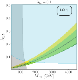
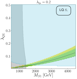
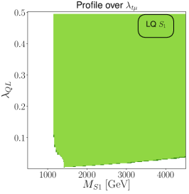
Figure 2: Scenarios which can explain $\Delta a_{\mu}^{\text{BNL}}$ and/or $\Delta a_{\mu}^{\text{2021}}$ in the model with an $SU(2)_{L}$ singlet scalar leptoquark $S_{1}$ defined in Eq. (18). Results are shown in the $M_{S1}$-$\lambda_{QL}$ plane for fixed $\lambda_{t\mu}=0.1$ (left panel), $\lambda_{t\mu}=0.2$ (middle panel) and by varying $\lambda_{t\mu}\in{\color[rgb]{0,0,0}[0,0.5]}$ (right panel). In the latter case we profile to find the regions in the $M_{S1}$-$\lambda_{QL}$ plane that for some value of $\lambda_{t\mu}$ in the scan, satisfy all experimental constraints and can explain the $\Delta a_{\mu}$ measurements within 1$\sigma$. Regions which can explain $\Delta a_{\mu}^{\textrm{BNL}}$ and $\Delta a_{\mu}^{\text{2021}}$ to within $1\sigma$ are yellow and green respectively, with the overlap between these two regions coloured lime. The black line indicates points which produce a $\Delta a_{\mu}$ contribution matching Eq. (7). The grey regions are excluded by scalar leptoquark searches at the Large Hadron Collider [440]. Regions shaded cyan are disfavoured as they provide a relative contribution which shift the muon mass up by more than $100\%$ or down by more than $50\%$ as in Eq. (22). In the right panel only solutions which have not been excluded by leptoquark searches or $Z\rightarrow\mu\mu$ or $Z\rightarrow\nu\nu$ constraints are displayed, i.e. any points ruled out by any of these experimental constraints are discarded.

The left and middle panels of Fig. 2 show where $\Delta a_{\mu}^{\text{BNL}}$ and $\Delta a_{\mu}^{\text{2021}}$ can be explained when the coupling to the right-handed top quark is fixed to $\lambda_{t\mu}=0.1,0.2$ respectively. For $\lambda_{t\mu}=0.1$, the black line showing points which exactly explain the $\Delta a_{\mu}^{\text{2021}}$ discrepancy is a parabolic curve, following the quadratic relationship between leptoquark mass and coupling in Eq. (28). By increasing the coupling to $\lambda_{t\mu}=0.2$, a lower value of the coupling $\lambda_{QL}$ to the left-handed top quark is required to get the same contributions to $\Delta a_{\mu}$, and the region which can explain $\Delta a_{\mu}^{\text{2021}}$ narrows and flattens as shown in the middle panel. In both cases the new $\Delta a_{\mu}^{\text{2021}}$ value can be explained with a marginally smaller coupling than the previous BNL value due to the small decrease in the discrepancy. CMS searches for scalar leptoquarks [440], shown by grey shading, exclude regions with masses $M_{S_{1}}\lesssim 1.1$–$1.5$ TeV, dependent on the branching ratio $\beta_{S_{1}}$ in Eq. (20). For lower $\lambda_{QL}$ couplings the strongest mass constraint of $M_{S_{1}}>1420$ GeV arises, since $\beta_{S_{1}}\rightarrow 1$ as $\lambda_{QL}\rightarrow 0$. Additionally, the cyan region indicates points affected by the “fine-tuning” in the muon mass discussed in Sec. 2 and defined in Eq. (22): here the loop contributions to muon mass calculated in FlexibleSUSY cause the muon mass to increase more than twice the pole mass or decrease less than half the pole mass. Satisfying this fine-tuning criteria, places a rough upper limit of $\lambda_{QL}\lesssim 0.06$ for $\lambda_{t\mu}=0.1$ and $\lambda_{QL}\lesssim 0.04$ for $\lambda_{t\mu}=0.2$. Note that these fine-tuning conditions allow only a small strip of the parameter space to remain.

In the right panel of Fig. 2, we profile over $\lambda_{t\mu}$ to find the best fits to $a_{\mu}$, that is we vary the coupling $\lambda_{t\mu}\in[0,0.5]$ and show the lowest number of standard deviation within which $a_{\mu}$ can be explained in the 2D plane, from all scenarios where $\lambda_{t\mu}\in[0,0.5]$. This panel has the same constraints as before, except for the muon mass fine-tuning. The LHC leptoquark searches impose a limit of $M_{S_{1}}\gtrsim 1.1$ TeV, with slightly higher mass limits implied by this for the lowest $\lambda_{QL}$ values since the branching ratios depend on the leptoquark couplings. The exclusion in the bottom right of the plot is formed by our choice of restricting the $\lambda_{t\mu}$ to moderate values $\leq 0.5$. If we allow $\lambda_{t\mu}$ to vary up to $\sqrt{4\pi}$ then no exclusion in the bottom right would be visible due to the large chirality flip enhancement. As the mass $M_{S_{1}}$ is increased, the minimum coupling $\lambda_{QL}$ which produces a contribution that can explain $a_{\mu}$ within $1\sigma$ increases, in line with Eq. (28), with the new world average result able to be explained in narrower region of the parameter space due to the reduction in the uncertainty.

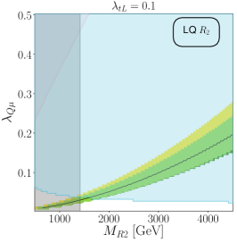
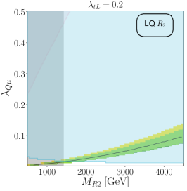
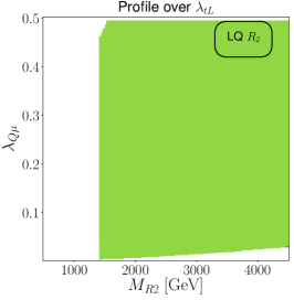
Figure 3: Scenarios which can explain $\Delta a_{\mu}^{\text{BNL}}$ and/or $\Delta a_{\mu}^{\text{2021}}$ in the model with a scalar leptoquark $SU(2)_{L}$ doublet $R_{2}$ defined in Eq. (19). Results are shown in the $M_{R2}$-$\lambda_{QL}$ plane for fixed $\lambda_{tL}=0.1$ (left panel), $\lambda_{tL}=0.2$ (middle panel) and by varying $\lambda_{tL}\in[0,0.5]$ (right panel). In the latter case we profile to find the regions in the $M_{R2}$-$\lambda_{QL}$ plane where these measurements can be explained for some value of $\lambda_{tL}$ in the scan and satisfy experimental constraints. Colours are the same as in Fig. 2. Additional relevant exclusions in the parameter space from the constraint $Z\rightarrow\nu\nu$ are shaded in pink and in the right panel this is included in the list of experimental constraints that points must satisfy, in addition to those listed in Fig. 2.

Similarly, for the scalar leptoquark doublet $R_{2}$, $\Delta a_{\mu}$ contours for fixed values of the coupling to right-handed top quarks, $\lambda_{tL}=0.1,0.2$, are shown in left and middle panels of Fig. 3, with a profile over $\lambda_{tL}$ shown in the right panel. Again, the $\Delta a_{\mu}$ contours for fixed $\lambda_{tL}=0.1,0.2$ follow the quadratic ratio given in Eq. (28), with larger $\Delta a_{\mu}$ values from a given leptoquark mass being obtained with the larger coupling $\lambda_{tL}=0.2$. This time, the mass constraints placed on the leptoquark $R_{2}^{u}$ from the LHC are independent of the couplings, as $R_{2}^{u}$ always decays to a top quark and muon. Again imposing the fine-tuning criteria has a huge impact, with the contributions from the leptoquark reducing the muon mass $m_{\mu}$. For $\lambda_{tL}=0.1$ only a small corner of parameter space can explain $\Delta a_{\mu}^{\text{2021}}$ without fine tuning, and for $\lambda_{tL}=0.2$ this shrinks to a tiny region. From profiling over $\lambda_{tL}$, we find that again $\Delta a_{\mu}^{\text{2021}}$ can be explained within $1\sigma$ for masses $M_{R_{2}}\geq 1420$ GeV. For higher couplings $\lambda_{Q\mu}\gtrsim 0.47$, constraints from $Z\rightarrow\nu\nu$ raise the minimum mass which can explain $\Delta a_{\mu}^{\text{2021}}$. As with the previous model our choice to restrict ourselves to moderate $\lambda_{tL}\leq 0.5$ leads a lower bound on the $\lambda_{Q\mu}$ coupling that increases with mass as a smaller coupling $\lambda_{Q\mu}$ cannot produce a large enough $\Delta a_{\mu}^{\text{2021}}$. As before there would be no exclusion in the bottom right region if we varied $\lambda_{tL}$ up to $\sqrt{4\pi}$.

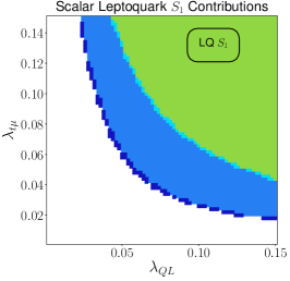
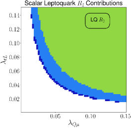
Figure 4: Results for $\Delta a_{\mu}^{\text{2021}}$ and $\Delta a_{\mu}^{\text{BNL}}$ in the planes of the leptoquark couplings where we profile over all possible scalar leptoquark masses up to $4.5$ TeV. More specifically in the left panel we show results for the $SU(2)_{L}$ singlet $S_{1}$ defined in Eq. (18) in the $\lambda_{QL}$–$\lambda_{t\mu}$ plane and in the right panel we show the scalar leptoquark $SU(2)_{L}$ doublet $R_{2}$ defined in Eq. (19) in the $\lambda_{Q\mu}$–$\lambda_{tL}$ plane. We show couplings between the leptoquark and the SM fermions that can satisfy direct LHC searches and $Z\rightarrow\mu\mu$ and $Z\rightarrow\nu\nu$ constraints and can simulteneously explain $\Delta a_{\mu}^{\text{2021}}$ (green) or both $\Delta a_{\mu}^{\textrm{BNL}}$ and $\Delta a_{\mu}^{\text{2021}}$ (lime green) within $1\sigma$. Additionally points which can also avoid the fine-tuning constraints in Eq. (22) on the muon mass are shaded in dark blue if they can explain $\Delta a_{\mu}^{\text{2021}}$, aqua if they can explain $\Delta a_{\mu}^{\textrm{BNL}}$ within $1\sigma$, and blue if they can explain both.

In Fig. 4 the $\Delta a_{\mu}$ predictions for both leptoquarks were profiled over the mass of the leptoquark with couplings ranging up to a cutoff of $0.5$, where we have again excluded points ruled out by the LHC searches and the decays $Z\rightarrow\mu\mu$ or $\nu\nu$. The regions which can explain $\Delta a_{\mu}^{\text{2021}}$ follow the relationship given in Eq. (28), where the contribution has identical dependence on the couplings to the left- and right-handed top quarks. As expected LHC limits on the leptoquark mass mean that there is a lower limit for the values of the couplings that can explain the observed $a_{\mu}$ disagreement within $1\sigma$. However, this limit is extremely small so that only leptoquarks with couplings $\lambda_{QL}\times\lambda_{t\mu}\lesssim 0.003$ are unable to produce large enough contributions to $a_{\mu}$ with a mass that has not be excluded by LHC searches in the $S_{1}$ model. As can be seen in the plot we obtain slightly lower limits on the couplings in the $R_{2}$ model compared to the $S_{1}$ model. This is due to the higher limits from the LHC on the leptoquark singlet at low couplings, as seen in Figs. 2, 3. Note that if we try to explain $\Delta a_{\mu}^{\textrm{BNL}}$ or $\Delta a_{\mu}^{\text{2021}}$ while avoiding fine-tuning of the muon mass, then we get an upper limit on the couplings of $\lambda_{QL}\times\lambda_{t\mu}\lesssim 0.006$ for the $S_{1}$ model and $\lambda_{tL}\times\lambda_{Q\mu}\lesssim 0.004$ for the $R_{2}$ model. However, putting aside fine-tuning constraints the deviation between the SM prediction and the observed value of the anomalous magnetic moment of the muon can be explained within $1\sigma$, needing couplings of reasonable size no smaller than $\approx 0.05$ each.

There are many possibilities for detecting leptoquarks at collider experiments, including planned high-luminosity improvements at the LHC as well as several proposed colliders such as the HE-LHC [451], ILC [452], CLIC [453], CEPC [454], and the FCC-ee [455] and FCC-hh [456]. The contributions of scalar leptoquarks to decays and flavour-changing processes such as $Z\rightarrow l_{i}l_{j}$, $Z\rightarrow\nu\nu$, $W\rightarrow l_{i}\nu$, $h\rightarrow l_{i}l_{j}$, $l_{i}\rightarrow l_{j}\gamma$, $l_{i}\rightarrow l_{j}\nu\nu$, and $l_{i}\rightarrow 3l_{j}$ have been examined by Ref. [272]. The authors found that the ILC, CLIC, CEPC, and FCC-ee may be sensitive to changes of the $Z\rightarrow l^{+}l^{-}$ couplings at the level of $10^{-5}-10^{-6}$ (relative to the standard coupling). They also estimated the ILC and FCC-ee sensitivity to branching fractions of $Z\rightarrow ll^{\prime}$ to be $10^{-8}-10^{-9}$. Ref. [457] examined the Higgs decays $h\rightarrow\gamma\gamma$, $h\rightarrow gg$ and $h\rightarrow Z\gamma$, and showed that the scalar leptoquarks contributions to these can generally be measured with increased precision at the ILC, CLIC, CEPC, FCC-ee and FCC-hh. They also showed that the value of the electroweak oblique observables, $S$ and $T$ (but not $U$), can change due to leading order contributions from scalar leptoquarks. They claimed that contributions to $T$ of size $0.01$ at the CEPC and $0.005$ at the FCC-ee could be measured. Ref. [458] calculated the production cross-sections of scalar leptoquark pairs and a scalar leptoquark with a lepton in proton-proton collisions at the LHC, HL-LHC, and HE-LHC colliders. The cross sections of leptoquark pair production at the HE-LHC and FCC-hh were also given by Ref. [459]. Ref. [435] was able to place an upper limit of $M_{LQ}<65$ TeV on the mass of the leptoquarks if one requires them to explain $\Delta a_{e}$ simultaneously with $\Delta a_{\mu}$. Additionally, other leptoquarks have also been shown to be detectable at collider experiments Ref. [460, 461, 462, 463, 464].

In summary leptoquarks are an exciting and well-motivated possibility for physics beyond the SM, which is not only motivated by $a_{\mu}$ but also by flavour anomalies. However, among all possible leptoquark quantum numbers, the $S_{1}$ and $R_{2}$ models are the only two viable explanations of $\Delta a_{\mu}^{\text{BNL}}$ and $\Delta a_{\mu}^{\text{2021}}$. Furthermore, leptoquark couplings of the left- and the right-handed muon to top quarks are required. In this way, chirality flip enhancements by $m_{t}/m_{\mu}$ are possible. Under these conditions, leptoquark masses above the LHC-limit of around $1.4$ TeV can accommodate $\Delta a_{\mu}^{\text{2021}}$ without violating flavour constraints. The large $\Delta a_{\mu}^{\text{2021}}$ can even be explained with leptoquark couplings to the left- and right-handed muon that are as small as $\approx 0.05$, which is essentially unchanged from the BNL value, despite the small reduction in the central value. In principle, masses in the multi-TeV region can accommodate the measured $a_{\mu}$, if the couplings are sufficiently increased. However, if one takes the fine tuning criteria on the muon mass seriously then only very narrow regions of parameter space remain for natural leptoquark solutions of the observed $a_{\mu}$, just above the LHC limits.

4 Two-Field Extensions

In this section we consider simple extensions of the SM by two fields. We focus on models where the new particles can appear together in pure BSM loops that contribute to $a_{\mu}$, in which case the new fields should have different spins. It is not possible to get an enhancement through internal chirality flips in these models, restricting explanations of $a_{\mu}$ to low mass regions, but compressed spectra in these regions may evade the LHC limits. In addition one of the new particles could be a stable dark matter candidate, and then simultaneous explanation of $a_{\mu}$ and dark matter is possible. For these reasons the case of two fields with different spins behaves very differently from the one-field extensions, and is representative for a range of more elaborate models.

We begin in Sec. 4.1 with an overview of the status of two-field extensions. There we also comment on the case with two fields of the same spin, including the interesting case of vector-like leptons. From the overview we identify two specific models that are promising in view of $a_{\mu}$, dark matter and LHC constraints. These models will be analysed in detail in Sec. 4.2 and compared against the latest $a_{\mu}^{\text{2021}}$ result and results from LHC and dark matter experiments.

4.1 Overview

$(SU(3)_{C}\times SU(2)_{L}\times U(1)_{Y})_{\textrm{spin}}$		$+\mathbb{Z}_{2}$	Result for $\Delta a_{\mu}^{\text{BNL}}$, $\Delta a_{\mu}^{\text{2021}}$
$({\bf 1},{\bf 1},0)$0	– $({\bf 1},{\bf 1},-1)$1/2	No	Projected LHC 14 TeV exclusion, not confirmed
		Yes	Updated Sec. 4.2
$({\bf 1},{\bf 1},-1)$0	– $({\bf 1},{\bf 1},0)$1/2	Both	Excluded: $\Delta a_{\mu}<0$
$({\bf 1},{\bf 2},-1/2)$0	– $({\bf 1},{\bf 1},0)$1/2	Both	Excluded: $\Delta a_{\mu}<0$
$({\bf 1},{\bf 1},0)$0	– $({\bf 1},{\bf 2},-1/2)$1/2	No	Excluded: LHC searches
		Yes	Updated Sec. 4.2
$({\bf 1},{\bf 2},-1/2)$0	– $({\bf 1},{\bf 1},-1)$1/2	No	Excluded: LEP contact interactions
		Yes	Viable with under abundant DM
$({\bf 1},{\bf 1},-1)$0	– $({\bf 1},{\bf 2},-1/2)$1/2	Both	Excluded: $\Delta a_{\mu}<0$
$({\bf 1},{\bf 2},-1/2)$0	– $({\bf 1},{\bf 2},-1/2)$1/2	Both	Excluded: LEP search
$({\bf 1},{\bf 2},-1/2)$0	– $({\bf 1},{\bf 3},0)$1/2	No	Excluded: LHC searches
		Yes	Viable with under abundant DM
$({\bf 1},{\bf 2},-1/2)$0	– $({\bf 1},{\bf 3},-1)$1/2	No	Excluded: LHC searches + LEP contact interactions
		Yes	Viable with under abundant DM
$({\bf 1},{\bf 3},0)$0	– $({\bf 1},{\bf 2},-1/2)$1/2	Both	Excluded: $\Delta a_{\mu}<0$
$({\bf 1},{\bf 3},0)$0	– $({\bf 1},{\bf 3},-1)$1/2	No	Excluded: LHC searches
		Yes	Viable with under abundant DM
$({\bf 1},{\bf 3},-1)$0	– $({\bf 1},{\bf 2},-1/2)$1/2	Both	Excluded: $\Delta a_{\mu}<0$
$({\bf 1},{\bf 3},-1)$0	– $({\bf 1},{\bf 3},0)$1/2	Both	Excluded: $\Delta a_{\mu}<0$
$({\bf 1},{\bf 1},-1)$1/2	– $({\bf 1},{\bf 1},0)$1	No	Excluded: $\Delta a_{\mu}<0$
$({\bf 1},{\bf 2},-1/2)$1/2	– $({\bf 1},{\bf 1},0)$1	No	Excluded: $\Delta a_{\mu}<0$
$({\bf 1},{\bf 2},-1/2)$1/2	– $({\bf 1},{\bf 3},0)$1	No	Excluded: LHC searches + LEP contact interactions
$({\bf 1},{\bf 1},0)$1/2	– $({\bf 1},{\bf 1},1)$1	No	Excluded: LHC searches + LEP contact interactions
$({\bf 1},{\bf 2},-1/2)$1/2	– $({\bf 1},{\bf 1},-1)$1	No	Excluded: LHC searches + LEP contact interactions
$({\bf 1},{\bf 3},-1)$1/2	– $({\bf 1},{\bf 3},0)$1	No	Excluded: $\Delta a_{\mu}<0$

Table 2: Summary of known results for gauge invariant extensions of two fields with different spin with one-loop contributions to the anomalous magnetic moment of the muon. These results are rather exhaustive due to systematic investigations and classifications in Refs. [367, 372, 376]. Note that this summarises results in the literature where different assumptions have been made, see the text and the original references for details. When there are multiple reasons for ruling a scenario out, we mention the most model- independent constraint. We use color highlighting to give a visual indication of the status of the model, namely green for viable explanations, red for excluded and purple for extensions that are only viable with under abundant dark matter.

With the possibilities for one-field extensions essentially exhausted, it is natural to then consider including two new fields entering the one-loop diagrams for $a_{\mu}$ together. The one-loop diagrams shown in Fig. 19 of Appendix A, have topologies FFS, SSF, VVF, FFV, VSF and SVF (where F $=$ fermion, S $=$ scalar and V $=$ vector boson). Clearly, having loops with only BSM particles requires that the two new states have different spin. One of the new states must be a fermion (allowed to be Dirac, Majorana or Weyl fermion), the other either a scalar or a vector boson. This means the new states can’t mix and new fermions can’t couple to both the left- and right-handed muon, so no new chirality flips may be introduced. Therefore $\Delta a_{\mu}^{\textrm{BNL}}$ explanations like this are heavily constrained and this has now been strongly confirmed with $\Delta a_{\mu}^{\text{2021}}$ result. Nonetheless one important new feature is that these both states couple to the muon together in trilinear vertices. If this is the only way they couple to SM states, and the BSM states have similar masses, then LHC limits could be evaded due to compressed spectra. Furthermore if this is due to a $\mathbb{Z}_{2}$ symmetry where the BSM states transform as odd, then it predicts a stable particle that could be a dark matter candidate.

The status of $\Delta a_{\mu}^{\textrm{BNL}}$ from a pair of BSM fields with different spins is summarised in Table 2, and these results have simply been confirmed by the new world average $\Delta a_{\mu}^{\text{2021}}$. This table draws extensively from Refs. [367, 372, 376]. Ref. [367] considers models without dark matter candidates and requires minimal flavour violation, while Refs. [372] and [376] consider models with ${\mathbb{Z}}_{2}$ symmetry and dark matter candidates. Many models can be immediately excluded because their contributions to $a_{\mu}$ are always negative with results in the literature in reasonable agreement regarding this. Models with positive contributions to $a_{\mu}$ predict a sufficiently large contribution only for very light states, and as a result collider searches place severe constraints on these models. However the collider search limits depend on the model assumptions and need to be understood in this context. The ${\mathbb{Z}}_{2}$ symmetry is particularly important as it regulates the interaction between the SM and BSM particles. Therefore, when necessary/required, the models in Table 2 are considered in two cases: with or without ${\mathbb{Z}}_{2}$ symmetry. Collider constraints effectively eliminate almost all the models without $\mathbb{Z}_{2}$ symmetry, while requiring that the $\mathbb{Z}_{2}$ symmetric models simultaneously explain dark matter and $\Delta a_{\mu}^{\textrm{BNL}}$ effectively restricts us to just the two models that we update in Sec. 4.2. However first, in the following, we explain the assumptions used in our main sources to eliminate the remaining models that give a positive contribution to $a_{\mu}$ and the important caveats to these findings.

The introduction of a vector-like fermion and a scalar or a vector without any additional symmetries was dealt with by Ref. [367], considering different $SU(2)_{L}$ representations, namely singlets, doublets, triplets or adjoint triplets. They quickly eliminate a scalar doublet and fermion doublet combination, i.e. $({\bf 1},{\bf 2},-1/2)$₀ – $({\bf 1},{\bf 2},-1/2)$_1/2, without considering LHC constraints because cancellations amongst the contributions mean $\Delta a_{\mu}$ is too small for a $1\sigma$ explanation of $\Delta a_{\mu}^{\textrm{BNL}}$ while satisfying basic assumptions like perturbativity and the $\approx 100$ GeV LEP limit [465, 466]. For LHC searches they look at Drell-Yan production, which depends only on the gauge structure, but for decays they rely on $\mathbb{Z}_{2}$ violating leptonic interactions where they assume a minimal flavour violating structure. They apply also LEP constraints on contact interactions, using the same assumptions for the lepton interactions. However one should again note the caveats described at the beginning of Sec. 3.1 on minimal flavour violation and abscence of scalar VEV. Adding only 8 TeV LHC searches effectively eliminates three more $\Delta a_{\mu}^{\textrm{BNL}}$ explanations: $({\bf 1},{\bf 1},0)$₀ – $({\bf 1},{\bf 2},-1/2)$_1/2, $({\bf 1},{\bf 2},-1/2)$₀ – $({\bf 1},{\bf 3},0)$_1/2 and $({\bf 1},{\bf 3},0)$₀ – $({\bf 1},{\bf 3},-1)$_1/2. Constraints on $ee\ell\ell$ contact interactions derived from LEP observables alone further excludes $({\bf 1},{\bf 2},-1/2)$₀ – $({\bf 1},{\bf 1},-1)$_1/2, and in combination with LHC searches excludes $({\bf 1},{\bf 2},-1/2)$₀ – $({\bf 1},{\bf 3},-1)$_1/2 and fermion-vector extensions $({\bf 1},{\bf 2},-1/2)$_1/2 – $({\bf 1},{\bf 3},0)$₁, $({\bf 1},{\bf 1},0)$_1/2 – $({\bf 1},{\bf 1},-1)$₁ and $({\bf 1},{\bf 2},-1/2)$_1/2 – $({\bf 1},{\bf 1},-1)$₁. It is important to also note that the limits from contact interactions can also be avoided by cancellations from the contributions of heavy states that may appear as part of a more elaborate model, and are therefore quite model dependent.

Ref. [372] considered scenarios with a new fermion and scalar, where there is a $\mathbb{Z}_{2}$ symmetry under which the BSM fields are odd, so that the models have a stable dark matter candidate. In all cases the dark matter candidate was the scalar. The new couplings they introduce are renormalizable, perturbative, CP conserving, gauge invariant and muon-philic (meaning that muons are the only SM fermions the BSM states couple to). For the scalar-fermion $({\bf 1},{\bf 1},0)$₀ – $({\bf 1},{\bf 1},-1)$_1/2 pair with charged fermion singlet, they find a region where $\Delta a_{\mu}^{\textrm{BNL}}$ and the relic density can both be explained within $2\sigma$. LHC constraints exclude much of the parameter space, but significant regions with compressed spectra survive. The results for the pair $({\bf 1},{\bf 1},0)$₀ – $({\bf 1},{\bf 2},-1/2)$_1/2 are essentially the same. We update both models in Sec. 4.2. For an inert scalar doublet, coupled with fermions that are $SU(2)_{L}$ singlets, doublets, triplets, i.e. $({\bf 1},{\bf 2},-1/2)$₀ – $({\bf 1},{\bf 1},-1)$_1/2, $({\bf 1},{\bf 2},-1/2)$₀ – $({\bf 1},{\bf 2},-1/2)$_1/2 and $({\bf 1},{\bf 2},-1/2)$₀ – $({\bf 1},{\bf 3},-1)$_1/2, they find a narrow region at, or just below, the Higgs resonance region ($m_{s}\approx m_{h}/2$), that is consistent with both the relic density and $a_{\mu}^{\textrm{BNL}}$ within $2\sigma$. LHC searches almost exclude these scenarios, but in all cases a tiny region where the fermion is about $100$ GeV survives. Since these regions are so small, in Table 2 we only report that these models are viable with under abundant dark matter. For an inert scalar doublet coupled with an adjoint triplet fermion ($({\bf 1},{\bf 2},-1/2)$₀ – $({\bf 1},{\bf 3},0)$_1/2) they find no region can be consistent $a_{\mu}^{\textrm{BNL}}$ and the observed DM relic density.

Ref. [376] considered the same type of models, but substantially expanded the number by including a wider range of dark matter candidates and systematically classifying the representations in a manner similar to that shown in our Table 2. For a given mass of the dark matter candidate that is sufficiently heavier than the $W$-boson mass, higher $SU(2)_{L}$ representations will have a comparatively large dark matter annihilation cross-section, they use this to place further analytically derived constraints on the models. Beyond the very fine tuned regions near the Higgs resonance the only models that could explain $\Delta a_{\mu}^{\textrm{BNL}}$ and the relic abundance of dark matter are scalar singlet dark matter with either a fermion singlet or fermion doublet, i.e. $({\bf 1},{\bf 1},0)$₀ – $({\bf 1},{\bf 1},-1)$_1/2 and $({\bf 1},{\bf 1},0)$₀ – $({\bf 1},{\bf 2},-1/2)$_1/2. For these two surviving explanations of dark matter and $\Delta a_{\mu}^{\textrm{BNL}}$ they further apply constraints from the $8$ TeV and $13$ TeV LHC searches and LEP limit on electroweak states. While in the latter model one can also get a neutral dark matter candidate if the fermion is lighter than the scalar, direct detection rules this out. They find that LHC searches heavily constrain the regions where relic density and $\Delta a_{\mu}^{\textrm{BNL}}$ may be simultaneously explained, but cannot entirely exclude the possibility.

4.1.1 Vector-like leptons

Before ending this overview we briefly also discuss the case of models with two fields of the same spin. In this case mixing of fields and enhanced chirality flips are allowed, but a dark matter candidate is precluded. Particularly interesting examples are extensions with vector-like leptons (VLLs), i.e. extension by two new vector-like fermions with the same quantum numbers as the left- and right-handed SM leptons. The muon-philic VLLs can couple both to left- and right-handed muons and to the Higgs boson; the contributions to $a_{\mu}$ behave similarly to the ones of leptoquarks in Eq. (28), but the chirality flip at the top quark is replaced by the new Yukawa coupling of the VLL to the Higgs boson. Such models have been discussed in detail in Refs. [293, 294, 296].

A distinguishing property of such models is that significant new contributions to the muon mass arise at tree level via the mixing with the new VLL. The relation between loop contributions to $a_{\mu}$ and to the tree-level muon mass is therefore more complicated than in the discussion of Sec. 2 leading to Eq. (12): for Higgs-loop contributions to $a_{\mu}$, the ratio between $\Delta a_{\mu}$ and $\Delta m_{\mu}^{\text{tree}}$ does not behave as $1/M_{\text{BSM}}^{2}$ but rather as $1/(16\pi^{2}v^{2})$ [293, 294]. Nevertheless, for couplings in line with electroweak precision constraints and perturbativity, only masses up to the TeV scale are able to provide significant contributions to $a_{\mu}$, similar to the bound of Eq. (13).

Currently these models with a single VLL can accommodate all existing limits, but there are two noteworthy constraints. On the one hand, bounds from $\mu\to e\gamma$ require the VLL couplings to be non-universal, i.e. very much weaker to the electron than to the muon (to allow large enough contributions for $a_{\mu}^{\text{2021}}$) [296]. On the other hand, the muon–Higgs coupling is modified by the large tree-level contributions to the muon mass. Already the current LHC constraints on the Higgs decay rate $h\to\mu^{+}\mu^{-}$ imply upper limits on the possible contributions to $a_{\mu}$, and if future experiments measure the $h\to\mu^{+}\mu^{-}$ rate to be in agreement with the SM prediction, a deviation as large as $\Delta a_{\mu}^{\text{BNL}}$ cannot be explained [296]. However extensions with more fields may relax the mass limits and constraints from $h\to\mu^{+}\mu^{-}$ [303, 304], given the lowest-order calculations of these references.

Slightly generalized models, where vector-like fermions may also carry quantum numbers different from ordinary leptons, have been examined in Refs. [367, 293]. Ref. [367] examined the introduction of a vector-like fermion $SU(2)_{L}$ doublet $({\bf 1},{\bf 2},-1/2)$ $\!\!{}_{1/2}$ with either an $SU(2)_{L}$ singlet ($({\bf 1},{\bf 1},0)$ $\!\!{}_{1/2}$ or $({\bf 1},{\bf 1},-1)$ $\!\!{}_{1/2}$) or a $SU(2)_{L}$ triplet ($({\bf 1},{\bf 3},0)$ $\!\!{}_{1/2}$ or $({\bf 1},{\bf 3},-1)$ $\!\!{}_{1/2}$). Each BSM fermion state is coupled to the Higgs boson and either the SM lepton $SU(2)_{L}$ doublet $L_{i}$, the SM lepton $SU(2)_{L}$ singlet $e_{i}$ with a flavour-universal coupling, or another BSM vector-like fermion. BSM and SM fermions of the same charge then mix together, with the amount of mixing between the SM and fermion states constrained by LEP limits [467]. Thus they allow minimal flavour violation between the SM lepton generations, and some of the main constraints on the masses of the vector-like fermions comes from minimal flavour violation. Ref. [293] additionally considered the introduction of a vector-like fermion $SU(2)_{L}$ doublet with hypercharge $Y=-3/2$ with either a charged fermion singlet or triplet (either $({\bf 1},{\bf 2},-3/2)$_1/2 – $({\bf 1},{\bf 1},-1)$_1/2 or $({\bf 1},{\bf 2},-3/2)$_1/2 – $({\bf 1},{\bf 3},-1)$_1/2). Ultimately both consider that these mixing vector-like fermions can produce positive contributions to $a_{\mu}$ and cannot be ruled out even by $14$-TeV LHC projections.

4.2 Scalar singlet plus fermion explanations

Our overview has resulted in two kinds of two-field models of particular interest, shown in Table 2. Both models are heavily constrained by LHC, but have not been excluded yet in the literature. We denote the two models as Model L and Model R, which extend the SM by adding the following fields:

$$\text{Model L:}\quad\phi,\ \psi_{d}=\begin{pmatrix}\psi_{d}^{+}\\ \psi_{d}^{0}\end{pmatrix},\, \text{Model R:}\quad\phi,\ \psi_{s}\equiv\psi_{s}^{-},$$ (29)

where $\phi=\phi^{0}$ is an $SU(2)_{L}$ singlet scalar field with representation $({\mathbf{1}},{\mathbf{1}},0)_{0}$, $\psi_{d}$ a doublet fermion field with representation $({\mathbf{1}},{\mathbf{2}},1/2)_{1/2}$, and $\psi_{s}$ a singlet fermion field with representation $({\mathbf{1}},{\mathbf{1}},-1)_{1/2}$. These new fermions are vector-like, or Dirac fermions, thus not only are the Weyl spinors $\psi_{d}$ and $\psi_{s}$ introduced but also their Dirac partners $\psi^{c}_{d}=(\psi_{d}^{+c\dagger},\psi_{d}^{0c\dagger})$ and $\psi_{s}^{c}\equiv\psi_{s}^{-c\dagger}$. In Model L the new fields couple only to the left-handed muon, and in Model R to the right-handed muon.

The two models add the following terms to the SM Lagrangian, using Weyl notation as in Eq. (19):

$${\cal L}_{\text{L}} =\begin{pmatrix}\lambda_{L}L\cdot\psi_{d}\phi-M_{\psi}\psi_{d}^{c}\psi_{d}+h.c.\end{pmatrix}-\frac{M_{\phi}^{2}}{2}|\phi|^{2},$$ (30)

$${\cal L}_{\text{R}} =\begin{pmatrix}\lambda_{R}\mu\phi\psi_{s}-M_{\psi}\psi_{s}^{c}\psi_{s}+h.c.\end{pmatrix}-\frac{M_{\phi}^{2}}{2}|\phi|^{2},$$ (31)

which can be written out into their $SU(2)_{L}$ components:

$${\cal L}_{\text{L}} =\begin{pmatrix}\lambda_{L}\nu_{\mu L}\psi_{d}^{0}\phi^{0}-\lambda_{L}\mu_{L}\psi_{d}^{+}\phi^{0}-M_{\psi}\psi_{d}^{0c\dagger}\psi_{d}^{0}-M_{\psi}\psi_{d}^{+c\dagger}\psi_{d}^{+}+h.c.\end{pmatrix}-\frac{M_{\phi}^{2}}{2}|\phi^{0}|^{2},$$ (32)

$${\cal L}_{\text{R}} =\begin{pmatrix}\lambda_{R}\mu_{R}^{\dagger}\psi_{s}^{-}\phi^{0}-M_{\psi}\psi_{s}^{-c\dagger}\psi_{s}^{-}+h.c.\end{pmatrix}-\frac{M_{\phi}^{2}}{2}|\phi^{0}|^{2}.$$ (33)

We have not included additional renormalisable terms involving the scalar singlet in the Higgs potential, which are not relevant for $a_{\mu}$, but we do briefly comment on the impact they would have later on, as they can affect the dark matter phenomenology. This leaves both models with just three parameters.

In the following we therefore present a detailed update of the phenomenology of Model L and Model R, scanning over all three parameters in each case to test whether or not dark matter and large $\Delta a_{\mu}$ can be simultaneously explained. We include the latest data from Fermilab, and the most recent LHC collider searches included in SModelS $1.2.3$ in Ref. [468, 469, 470, 471, 472, 473, 474] and CheckMate $2.0.26$ [475, 476, 477, 478, 479, 480, 481]. It should be noted that we deal only with BSM fields that couple to second generation SM fermions. Thus, flavour violation constraints on our models can safely be ignored, including limits from contact interactions. This is in line with the methodology in Ref. [376], but not [367].

The BSM contributions from both of the two field dark matter models come from the FFS diagram 19(a) of Fig. 19 with the generic $F$ fermion lines replaced by $\psi^{-}$ and the scalar $S$ one by $\phi^{0}$. The contributions to $a_{\mu}$ from both of these models are given by identical expressions (where $\lambda_{L,R}$ are generally denoted by $\lambda$). The result is given by

$$\Delta a_{\mu}^{\text{Model L}}=\Delta a_{\mu}^{\text{Model R}}=-Q_{\psi}\frac{\lambda^{2}}{32\pi^{2}}\frac{m_{\mu}^{2}}{6M_{\phi}^{2}}\,E\!\begin{pmatrix}\frac{M_{\psi}^{2}}{M_{\phi}^{2}}\end{pmatrix},$$ (34)

where $Q_{\psi}=-1$. It does not involve a chirality flip enhancement, which has a large impact on the ability of these models to explain $a_{\mu}$ whilst avoiding collider constraints.

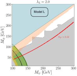
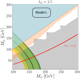
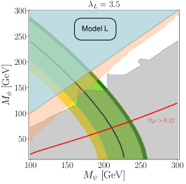
Figure 5: Results from Model L, scanning over the masses of the new fermion and scalar which couple to the left-handed muon. Regions which can explain $\Delta a_{\mu}$ in Eq. (7) or Eq. (6) to within $1\sigma$ are coloured green and yellow respectively, with the overlap between the two regions is coloured lime. The black line indicates masses which produce a $\Delta a_{\mu}$ contribution matching Eq. (7). The points where a dark matter candidate particle produces the observed relic abundance of $0.1200$, Eq. (8), are shown in red, with the region below being excluded due to having an over abundance of dark matter. The region where $M_{\psi}<M_{\phi}$ is shaded cyan. Regions excluded by $13$-TeV results at the LHC are shaded grey, with the exclusions from the soft leptons search [482] obtained using CheckMate shaded in orange. Thus $a_{\mu}$ can only be explained in small slices of parameter space between the grey and orange regions. As the coupling between the left-handed muon and the BSM particles is increased, higher masses are required to explain $a_{\mu}$.

The results for the first of the two field dark matter models, Model L, are shown in Figs. 5, 6. Scans were performed over a grid of scalar mass $M_{\phi}\in[0,400]$ GeV and fermion masses of $M_{\psi}\in[100,400]$ GeV, taking into consideration the LEP limit $M_{\psi}>100$ GeV [465, 466] on charged fermion masses. Before showing results of the full scan, in Fig. 5 we show $\Delta a_{\mu}$ in three slices of the parameter space in the $M_{\psi}$–$M_{\phi}$ ($M_{\psi}$ over $100...300$ GeV and $M_{\phi}$ over $0...300$ GeV) with fixed $\lambda_{L}=2,2.5,3.5$. Due to the lack of enhanced chirality flips a sufficiently large $\Delta a_{\mu}$ is obtained only when the coupling constant is large and the masses are relatively small. However due to the new reduced measurement of $a_{\mu}$, the discrepancy can be explained with heavier masses than before as indicated in the green curve. For $\lambda_{L}\leq 2$, the model cannot provide large enough $\Delta a_{\mu}$ to explain the anomaly within $1\sigma$ while avoiding the LEP $M_{\psi}>100$ GeV limit and LHC limits (discussed below), while for very large values of $\lambda_{L}=2.5$ or $\lambda_{L}=3.5$ it is possible to explain the anomaly but even when $\lambda_{L}$ is close to $\sqrt{4\pi}$, $\Delta a_{\mu}^{\text{2021}}$ can only be explained within $1\sigma$ for masses below $260$ GeV. These results can be approximately reproduced using Eq. (34), though we have again performed the calculation with FlexibleSUSY 2.5.0 [43, 44], which includes the full one-loop calculation and the universal leading logarithmic two-loop QED contribution [450].

We do not consider scenarios with $M_{\psi}<M_{\phi}$ because such cases are like Higgsino dark matter or the doublet case of minimal dark matter and as such will be under abundant when the mass is below about $1$ TeV (see e.g. Ref. [483]). Without a chirality flipping enhancement it will not be possible to explain $\Delta a_{\mu}^{\text{BNL}}$ or $\Delta a_{\mu}^{\text{2021}}$ with masses that are heavy enough to explain dark matter. Hence the dark matter candidate is given by the scalar singlet $\phi$. Direct detection of dark matter constraints then depend on the parameters of Higgs potential terms involving the singlet. By including such terms, we found that direct detection constraints rule out significant parts of the parameter space but can always be evaded by choosing the additional parameters to be small. Therefore, for simplicity, we neglect these parameters in our final numerical results and do not show direct detection constraints.

The collider constraints are shown with overlayed shading. The lower grey shaded region comes from searches for charginos, neutralinos, sleptons, and long-lived particles, using leptonic final states in the $8$-TeV searches [484, 485, 423, 486] and the $13$-TeV searches [487, 488, 489, 490], included in SModelS $1.2.3$ [491, 492] and excludes most of the light mass parameter space where $a_{\mu}$ can be explained. Nonetheless there is still a considerable gap close to the $M_{\phi}=M_{\psi}$ line, which escapes these constraints, but may be closed by searches for compressed spectra. We therefore also show in shaded orange the CMS search for the compressed spectra of soft leptons [482], which was obtained using CheckMate $2.0.26$ [475, 476] using MadAnalysis [493] and PYTHIA [472, 473] to generate event cross-sections. As a result of these constraints there is little room for the model to evade collider constraints and explain the observed value of $a_{\mu}$, though some gaps do evade the collider constraints we apply.

Finally we also consider the relic density of dark matter in this model using micrOMEGAs $5.2.1$ [494]. The red line in Fig. 5 indicates where the model’s dark matter candidate particle produces the Planck-observed relic density of $\Omega_{h^{2}}=0.1200$, Eq. (8). Along this red line the relic abundance of dark matter is depleted to the observed value through t-channel exchange of the BSM fermions. This mechanism is less effective below the line, where the mass splitting between the BSM scalar and fermion is larger, leading to over abundance. All points below the red line are strongly excluded by this over abundance, though this does not rule out any scenarios that are not already excluded by collider constraints. Above the line the relic density is under abundant. Our results show that it is not possible for any of these $\lambda_{L}$ values to simultaneously explain $a_{\mu}^{\text{2021}}$ and the relic density, while evading collider limits.

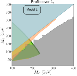
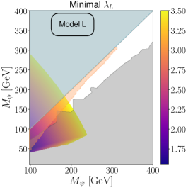
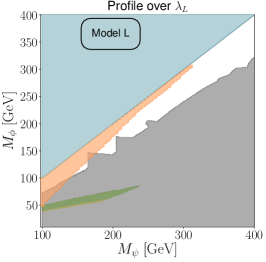
Figure 6: Several profiles of Model L. Colours for the first and third panels are the same as Fig. 5, and the same LHC limits (which do not depend on the coupling) are overlaid. The left panel shows the best contributions to $a_{\mu}$ for each value of the BSM masses, without having a dark matter candidate particle with an over abundant relic density. Likewise, the right panel only shows points which have a dark matter relic density within $1\sigma$ of the Planck observation [416]. The middle panel shows the smallest value of the coupling $\lambda_{L}$ which can explain $a_{\mu}^{\text{2021}}$ (Eq. (7)) within $1\sigma$ without producing over abundant dark matter.

To give a more global picture of the status of the model in Fig. 6 we also vary $\lambda_{L}\in[0,3.5]$. In the left panel we show where on the $M_{\phi}$–$M_{\psi}$ plane it is possible to simultaneously fit the BNL measurement or the new world average for $a_{\mu}$ and avoid an over abundant relic density, for some value of $\lambda_{L}$ within this range. As expected this shows that $\lambda_{L}$ may be adjusted so that for very light masses one may always explain $a_{\mu}$ within $1\sigma$, but as the masses are raised past $200-300$ GeV, this is no longer possible. As a result the combination of collider constraints shown in grey, cyan and orange exclude all but two narrow regions of parameter space in the compressed spectra region between the $M_{\phi}$ and $M_{\psi}$ masses. As shown in the middle panel of Fig. 6, where we plot the minimum value of $\lambda_{L}$ consistent with a $1\sigma$ explanation of $\Delta a_{\mu}^{\text{2021}}$, explaining the observed value requires a very large coupling $\lambda_{L}\geq 2.5$. One may question the precision of our calculation for such large values of $\lambda_{L}$, however given the mass reach of the collider experiments which extends well past the $1\sigma$ region it is unlikely that including higher orders in the BSM contributions will change anything significantly. Finally the right panel of Fig. 6 shows $a_{\mu}$ results that are compatible with explaining the full observed dark matter relic density within $1\sigma$, having obtained this data from a targeted scan using MultiNest 3.10 [495, 496, 497, 498]. Our results show that it is now impossible to simultaneously explain dark matter and $\Delta a_{\mu}^{\text{BNL}}$ and the same is true with the updated $\Delta a_{\mu}^{\text{2021}}$ measurement.

Compared to the results for this model shown in Ref. [376], we find that the most recent collider search(es) [485, 488], are the most important for narrowing the gaps in the exclusion. Currently, there is very little room for the model to survive.

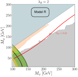
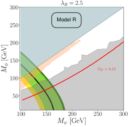
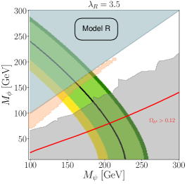
Figure 7: Results from Model R, scanning over the masses of the new fermion and scalar which couple to the right-handed muon. Colours are the same as Fig. 5.

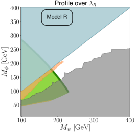
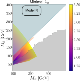
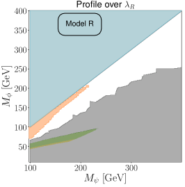
Figure 8: Several profiles of Model R. Colours for the first and third panels are the same as Fig. 5. The middle panel shows the lowest value of $\lambda_{R}$ which can explain $a_{\mu}^{\text{2021}}$ from Eq. (7) within $1\sigma$. The panels are constructed in the same way as those in Fig. 6. The same LHC limits as Fig. 7 (which do not depend on the coupling) are overlaid.

Results for Model R are shown in Figs. 7, 8. Since the contributions to $a_{\mu}$ for this model are also governed by Eq. (34), the behaviour of $\Delta a_{\mu}$ is the same. However as one can see in Figs. 7, 8 the collider constraints for Model R, which has no $SU(2)_{L}$ interactions, are weaker than those for Model L, with the exclusions again coming from SModelS 1.2.3 through the $8$-TeV searches [485, 499, 500, 486] and the $13$-TeV searches [487, 488, 490, 489, 501]. The searches providing most of the constriction on the parameter space of Model R are the ATLAS searches [485, 490] and the CMS searches [501, 488]. As a result in the case of Model R there is still some room to explain the $a_{\mu}$ measurement within currently applied collider constraints. However as can be seen in the left panel of Fig. 7 even with $\lambda_{R}=2.0$, there is only a little room to escape the combination of the standard electroweakino searches shaded grey and the soft lepton compressed spectra search shaded orange. In the middle panel when $\lambda_{R}=2.5$ one can see a significantly larger, but still narrow region where $a_{\mu}^{\text{2021}}$ can be explained within $1\sigma$ while evading the collider limits. In the right panel as $\lambda_{R}$ approaches the perturbative limit both the value and area of the viable parameter space are larger. In the left panel of Fig. 8, where $\lambda_{R}$ is allowed to vary, one can see the full region of the $M_{\phi}-M_{\psi}$ plane where $a_{\mu}^{\text{2021}}$ is explained within $1\sigma$, while avoiding giving a relic density of dark matter which is too over abundant. With the overlaid collider limits we can see the complete picture of parameter space where it remains possible to explain this observed $a_{\mu}$, while evading limits from colliders. Avoiding collider constraints from the LHC requires compressed spectra, and comparing the green and lime green regions, one can see that the situation with the new world average has just marginally increased the masses that can be accommodated. However as shown by the middle panel of Fig. 8, evading these limits requires a coupling of $\lambda_{R}\gtrsim 1.8$. One can also see that the relic density cannot be explained simultaneously with $a_{\mu}^{\text{2021}}$ in any of the slices shown in Fig. 7, and the right panel of Fig. 8 does show that the regions which can explain dark matter relic density and $\Delta a_{\mu}^{\text{2021}}$ to within $1\sigma$ are fully ruled out by collider constraints.

In summary, two-field models with different spin do not contain new sources of chirality flipping enhancements, and many models of this class are not able to generate significant positive contributions to $a_{\mu}$, see Table 2. However the Model L and Model R investigated here do give positive contributions, and our results show they remain viable explanations of the new world average deviation $\Delta a_{\mu}^{\text{2021}}$ after the FNAL measurement, as can be seen from Figs. 5-8, with small parts of the parameters space escaping LHC constraints. Model R is found to be slightly more viable due to reduced impact of LHC constraints, in particular those from compressed spectra searches. In both models, however, it is not possible to simultaneously explain $\Delta a_{\mu}^{\text{2021}}$ whilst producing the observed dark matter relic density [416] and satisfying LHC collider constraints. It is only possible to explain $\Delta a_{\mu}^{\text{2021}}$ within $1\sigma$ with an under abundant dark matter candidate particle. Further, the lack of chirality flip for either of these models constrain the masses to be $M_{\psi},M_{\phi}\leq 210$ GeV to both avoid collider constraints and explain the value of $\Delta a_{\mu}^{\text{2021}}$, where compressed spectra searches are important for the viability of these models. Future data from $a_{\mu}$ experiments and LHC might entirely exclude these models.

5 Three-Field Extensions

As we saw in Sec. 4 introducing two fields with different spins is the simplest way to explain dark matter and give new contributions to muon $g-2$, but collider constraints heavily constrain the region where such models can explain the observed muon $g-2$. This is because in those cases it is not possible to induce a chirality flip in the muon $g-2$ diagram’s loop, as both the new fermion and scalar only couple to either the left- or right-handed muon.

We therefore now consider the simplest models that can both have an enhanced contribution to muon $g-2$ from a chirality flip and explain dark matter. These are models with two fields of the same spin that mix together and a third field with a different spin and a $\mathbb{Z}_{2}$ symmetry under which these new fields are odd, while the SM fields are even. The leading contributions in supersymmetric models are in fact of this kind, as will be discussed in Sec. 6, but here we also consider three-field models that do not arise as part of the MSSM. As in previous sections we will restrict ourselves to renormalizable models with new scalars and new fermions. Models of this nature have previously been classified in Ref. [376], and there it is demonstrated that due to the chirality flip contribution there are many models which can explain the $a_{\mu}$ anomaly in Eq. (6), with models that have a new field with a much higher $SU(2)_{L}$ representation (up to $20$) being able to produce sizable contributions to $a_{\mu}$. Likewise, the larger contributions to $a_{\mu}$ from the chirality flip enables three field models to simultaneously produce a dark matter candidate with the observed dark matter relic abundance [502] also with much higher $SU(2)_{L}$ representations compared to the two field models. This chirality flip enhancement also enables one to examine much higher mass scales compared to two field models, evading LHC collider constraints.

In this section we present a detailed discussion of the phenomenology of two kinds of three-field models, which we denote as 2S1F and 2F1S, with two scalars and one fermion or vice versa. The quantum numbers will be chosen such that the models represent a variety of possible dark matter candidates. In model 2S1F, the dark matter is a scalar singlet or doublet (or mixture) and may be compared to generic scalar singlet or inert doublet models or to left- or right-handed sneutrinos. In model 2F1S, the dark matter is a singlet or doublet fermion (or a mixture) and may be compared to Bino or neutral Higgsino. Model 2S1F has some similarities to the BLR contribution in the MSSM, but the spin of the dark matter candidate is different. Model 2F1S contains the same states as the BHL contribution in the MSSM. In both cases, the couplings are treated as arbitrary, not respecting SUSY-like relations, which leads to a different phenomenology, and we compare and contrast these two models with their respective MSSM scenarios. Both of these models were considered in Ref. [376], showing particular slices of the parameter space. Here we update these models with the latest $a_{\mu}^{\text{2021}}$ result and direct detection constraints, and perform a thorough sampling of the whole parameter space to show how the data leads to meaningful constraints on the parameters of these models.

5.1 Three-field model with two scalars, one charged fermion and scalar dark matter

We begin with the Model 2S1F which is the SM extended with three ${\mathbb{Z}}_{2}$-odd fields: one electrically charged fermion and two scalar fields,

$$\psi_{s},\quad\phi_{s}^{0},\quad\phi_{d}=\begin{pmatrix}\frac{\phi^{0}_{d}+iA_{\phi}}{\sqrt{2}}\\ \phi_{d}^{-}\end{pmatrix}\,,$$ (35)

where $\psi_{s}$ is an $SU(2)$ singlet charged Dirac fermion expressed in Weyl spinors with representation $({\bf{1}},{\bf{1}},1)_{1/2}$, $\phi_{s}^{0}$ a scalar singlet with representation $({\bf{1}},{\bf{1}},0)_{0}$, and $\phi_{d}$ a scalar doublet with representation $({\bf{1}},{\bf{2}},-\frac{1}{2})_{0}$. The relevant interactions are:

$${\cal L}_{\text{2S1F}}=\begin{pmatrix}a_{H}H\cdot\phi_{d}\phi_{s}^{0}+\lambda_{L}\phi_{d}\cdot L\psi_{s}+\lambda_{R}\phi_{s}^{0}\mu\psi_{s}^{c}-M_{\psi}\psi_{s}^{c}\psi_{s}+h.c.\end{pmatrix}-M_{\phi_{d}}^{2}|\phi_{d}|^{2}-\frac{M_{\phi_{s}}^{2}}{2}|\phi_{s}^{0}|^{2}.$$ (36)

The new scalars couple to one of the left- and right-handed muons each, along with the new fermion. Then using a trilinear scalar coupling between the two scalars and the Higgs boson, the VEV of the Higgs bosons gives rise to mass mixing terms between the two scalars, and induces a chirality flip in the loop of muon $g-2$ processes. The relevant parameter combination for invoking this chirality flip enhancement is $a_{H}\lambda_{L}\lambda_{R}$.

For Model 2S1F in Eq. (36), the neutral scalar singlet $\phi_{s}^{0}$ and the CP-even part of the neutral component of $\phi_{d}$ mix together into two flavours of a neutral scalar $\phi^{0}_{i}$ for $i=1,2$:

$${\cal L}_{\text{2S1F}}\ni-\frac{1}{2}\begin{pmatrix}\phi_{s}^{0}&\phi_{d}^{0}\end{pmatrix}\begin{pmatrix}M_{\phi_{s}}^{2}&a_{H}v\\ a_{H}v&M_{\phi_{d}}^{2}\end{pmatrix}\begin{pmatrix}\phi_{s}^{0}\\ \phi_{d}^{0}\end{pmatrix} =-\frac{1}{2}\sum_{i=1,2}M^{2}_{\phi_{i}^{0}}|\phi_{i}^{0}|^{2},$$

where the mass eigenstates relate to the gauge eigenstates through the mixing matrix $U_{S}$ as

$$\begin{pmatrix}\phi_{1}^{0}\\ \phi_{2}^{0}\end{pmatrix} =U_{S}^{T}\begin{pmatrix}\phi_{s}^{0}\\ \phi_{d}^{0}\end{pmatrix}\,.$$ (37)

The dark matter candidate is then the lightest neutral scalar $\phi^{0}_{1}$. For this mixing to avoid producing a tachyon, the limit $a_{H}v<M_{\phi_{s}}M_{\phi_{d}}$ must be respected. As in the previous section on two-field extensions, we do not consider additional renormalisable terms involving the new scalars that could appear in the Higgs potential, but would not affect the $a_{\mu}$ prediction. These terms can change the dark matter phenomenology though, adding additional mechanisms to deplete the relic density, and new interactions that can mediate direct detection. However we do not expect these to substantially modify our conclusions.

In this model the one-loop BSM contribution to the anomalous magnetic moment is given by:

$$\Delta a_{\mu}^{\text{2S1F}}= \frac{m_{\mu}^{2}}{32\pi^{2}}\bigg{(}\frac{\lambda_{L}^{2}}{12M_{\phi_{d}}^{2}}\,E\!\begin{pmatrix}\frac{M_{\psi}^{2}}{M_{\phi_{d}}^{2}}\end{pmatrix}+\sum_{i=1,2}\frac{\lambda_{L}^{2}|U_{S\,2i}|^{2}+2\lambda_{R}^{2}|U_{S\,1i}|^{2}}{12M_{\phi_{i}^{0}}^{2}}\,E\!\begin{pmatrix}\frac{M_{\psi}^{2}}{M_{\phi_{i}^{0}}^{2}}\end{pmatrix}$$

$$+\frac{M_{\psi}}{m_{\mu}}\sum_{i=1,2}\frac{2\sqrt{2}\lambda_{L}\lambda_{R}U_{S\,1i}U_{S\,2i}}{3M_{\phi_{i}^{0}}^{2}}\,F\!\begin{pmatrix}\frac{M^{2}_{\psi}}{M^{2}_{\phi_{i}^{0}}}\end{pmatrix}\bigg{)}.$$ (38)

These contributions come in the form of the FFS diagram 19(a) of Fig. 19 with the generic $F$ fermion lines replaced by $\psi^{-}$ the conjugate of $\psi_{s}$, and the scalar $S$ one by $\phi^{0}_{i}$ and $A_{\phi}$, respectively.

The second line of Eq. (5.1) provides the contribution with the chirality flip enhancement, and is therefore typically the dominant contribution. While a cursory glance at Eq. (5.1) might lead one to believe that this model’s chirality flip provides an apparent enhancement according to the ratio $M_{\psi}/m_{\mu}$, the actual behaviour is more complicated. The actual form of this enhancement can be seen by using the simplification of the mixing angles $U_{S\,11}U_{S\,21}=-U_{S\,12}U_{S\,22}\to a_{H}v/(M_{\phi_{1}^{0}}^{2}-M_{\phi_{2}^{0}}^{2})$. Plugging this into Eq. (5.1) generates a difference between loop functions which, together with the mass difference in the denominator, can be written in terms of the loop function $\tilde{F}_{a}$ of the appendix Eq. (90). In this way, for $M_{\psi}\gg m_{\mu}$, the contribution from this model simplifies to the chirality flip contribution as:

$$\Delta a_{\mu}^{\text{2S1F}}\approx \frac{m_{\mu}^{2}}{32\pi^{2}}\frac{M_{\psi}}{m_{\mu}}\sum_{i=1,2}\frac{2\sqrt{2}\lambda_{L}\lambda_{R}U_{S\,1i}U_{S\,2i}}{3M_{\phi_{i}^{0}}^{2}}\,F\!\begin{pmatrix}\frac{M^{2}_{\psi}}{M^{2}_{\phi_{i}^{0}}}\end{pmatrix}$$ (39)

$$\approx \frac{m_{\mu}^{2}}{32\pi^{2}}\frac{M_{\psi}}{m_{\mu}}\frac{2\sqrt{2}\lambda_{L}\lambda_{R}a_{H}v}{3(M_{\phi_{1}^{0}}^{2}-M_{\phi_{2}^{0}}^{2})}\left(\frac{1}{M^{2}_{\phi_{1}^{0}}}\,F\!\begin{pmatrix}\frac{M^{2}_{\psi}}{M^{2}_{\phi_{1}^{0}}}\end{pmatrix}-\frac{1}{M^{2}_{\phi_{2}^{0}}}\,F\!\begin{pmatrix}\frac{M^{2}_{\psi}}{M^{2}_{\phi_{2}^{0}}}\end{pmatrix}\right).$$ (40)

$$\approx -\frac{m_{\mu}^{2}}{32\pi^{2}}\frac{M_{\psi}}{m_{\mu}}\frac{2\sqrt{2}\lambda_{L}\lambda_{R}a_{H}v}{M_{\psi}^{4}}\,\tilde{F}_{a}\!\begin{pmatrix}\frac{M^{2}_{\psi}}{M^{2}_{\phi_{1}^{0}}},\frac{M^{2}_{\psi}}{M^{2}_{\phi_{2}^{0}}}\end{pmatrix}.$$ (41)

Thus the final result for this chirality-enhanced contribution can be written in the form

$$\Delta a_{\mu}^{\text{2S1F}}\approx -\frac{m_{\mu}^{2}}{32\pi^{2}M_{\psi}^{2}}\frac{}{}\frac{2\sqrt{2}\lambda_{L}\lambda_{R}a_{H}v}{m_{\mu}M_{\psi}}\,\tilde{F}_{a}\!\begin{pmatrix}\frac{M^{2}_{\psi}}{M^{2}_{\phi_{1}^{0}}},\frac{M^{2}_{\psi}}{M^{2}_{\phi_{2}^{0}}}\end{pmatrix},$$ (42)

where e.g. $\tilde{F}_{a}(1,1)=1/12$. We see that the actual enhancement factor, beyond the typical loop and mass suppression factor, is given by the ratio $\lambda_{L}\lambda_{R}a_{H}v/(m_{\mu}M_{\psi})$. As announced earlier it relies on the factor $\lambda_{L}\lambda_{R}a_{H}$ and requires all three of these couplings to be non-zero.

We have presented this discussion of how the parametric behaviour of the chirality flip can be extracted from the exact result Eq. (5.1) in quite some detail, and we remark that similar discussions can also be applied to other models, e.g. to the model 2F1S discussed later, or to MSSM contributions discussed in Sec. 6.

If either $\lambda_{L}$ or $\lambda_{R}$ are zero then clearly the above contribution vanishes, while it will also vanish if there is no mixing between the scalars, i.e. $a_{H}=0$, so that $U_{S\,1i}U_{S\,2i}$ vanishes. If $\lambda_{L}=a_{H}=0$ or $\lambda_{R}=a_{H}=0$ then Eq. (5.1) reduces to the same result for two fields with different spin, i.e. Eq. (34), while if $a_{H}$ is non-zero, then one gets a similar result, but with some dilution from the mixing. Similarly if both $\lambda_{L}$ and $\lambda_{R}$ are non-zero, but $a_{H}=0$ then we simply get two copies of Eq. (34), with different couplings that are summed. Finally note that the mixing will also be heavily suppressed just by having a large enough mass splitting between the two scalar states, i.e. making the ratio $(va_{H})^{2}/(M_{\phi_{s}}^{2}M_{\phi_{d}}^{2})$ sufficiently small.

In the following we provide a detailed phenomenological analysis of the Model 2S1F. The underlying question is whether the model can accommodate the new $a_{\mu}^{\text{2021}}$ value simultaneously with current constraints from dark matter and LHC. The model is complicated and depends on three masses and three couplings in a relevant way. We focus on the parameter space where $\lambda_{L}$, $\lambda_{R}$ and $a_{H}$ are all non-zero, such that the model behaves differently from the models of the previous section. Eq. (42) then provides the dominant contribution and can be used to understand our results. As in previous sections we do however use FlexibleSUSY 2.5.0 [43, 44] to obtain the numerical results, where we augment the full one-loop BSM calculation with the universal leading logarithmic photonic $2$-loop contributions [503].

Before entering details, we briefly explain relevant dark matter processes. Without the $a_{H}$, $\lambda_{L}$ and $\lambda_{R}$ interactions that are important for $a_{\mu}$, dark matter could behave either as pure scalar singlet or as pure inert scalar doublet dark matter. In the inert doublet case, already the standard SU(2)_L electroweak gauge interactions are sufficient to deplete the relic density to (below) the observed value when it has a mass of (less than) about $600$ GeV [504]. The preferred mass of scalar singlet dark matter depends on the Higgs portal coupling, but outside of fine tuned parameter regions and for couplings $\lambda_{L,R}<1$, the best fit for the data is found when the pure scalar singlet dark matter has a mass of $\approx 1$–$3$ TeV [505]. Beyond these simple special cases, the model here allows many additional depletion mechanisms: significant $\lambda_{L,R}$ allow t-channel exchange of the new fermion, through $\lambda_{L}$ or $\lambda_{R}$ if the scalar dark matter is doublet or singlet dominated (or both if there is mixing). If the new fermion mass is sufficiently close, coannihilations through $\lambda_{L}$ and $\lambda_{R}$ can also be active in depleting the relic density. The coupling $a_{H}$ between singlet, doublet, and the SM Higgs can lead to singlet–doublet coannihilation processes. This same coupling $a_{H}$ is also relevant for direct detection constraints on dark matter, which depend particularly on Higgs-mediated processes. Importantly, the mentioned additional depletion processes can compensate general suppressions of cross sections for heavier masses. As a result even heavier dark matter masses than for the inert doublet can become possible.

As we will see from detailed scans, the dark matter constraints indeed only allow rather heavy masses, which are above LHC limits. For this reason we do not explicitly consider LHC constraints in the following.

‘      

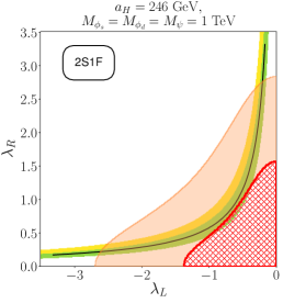
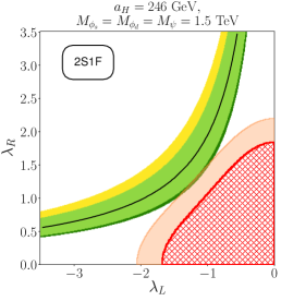
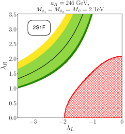
Figure 9: Results from Model 2S1F, scanning over the couplings of the new scalars and fermion to the left- and right-handed muon. All BSM fields have identical masses as specified in the subfigures. The trilinear coupling which parametrises the mixing of the neutral BSM scalars is fixed to $a_{H}=246$ GeV. Regions which can explain $\Delta a_{\mu}^{\textrm{BNL}}$ and $\Delta a_{\mu}^{\text{2021}}$ to within $1\sigma$ are coloured yellow and green respectively, while the overlap between these two regions is coloured lime. The black line marks couplings which produce a contribution which exactly matches Eq. (7). The points where a dark matter candidate particle produces the observed relic abundance of $0.1200$, Eq. (8), are at the boundary of the hatched region shown in red, with the hatched region below and to the right being excluded due to having a relic abundance greater than $0.12$. Regions excluded by searches for the direct detection of dark matter at the Xenon1T experiment[506, 507] are shaded in orange.

In Fig. 9 we begin our numerical analysis of this model. The figure represents a baseline behaviour. In order to maximize contributions to $a_{\mu}$ via a large chirality flip and mixing (see Eq. (42) and following discussion) we choose equal masses $M_{\phi_{s}}=M_{\phi_{d}}$ and fix $a_{H}=v=246$ GeV as a reference value, similar to scenarios examined by Ref. [376]. We also choose $M_{\psi}$ to be equal to the scalar masses. This is a rather special choice for dark matter, as all mechanisms for depleting the relic density can be active here, including scalar–fermion coannihilation. As a result, the relic density will be quite suppressed and the Planck-observed value can only be explained for small couplings. On the other hand, the dark matter direct detection will not be suppressed due to the large mixing between the scalar and doublet, allowing interactions with the nucleons through the moderately sized $a_{H}$ coupling.

The behaviour of $\Delta a_{\mu}$ in the three panels of Fig. 9 clearly reflects the $\lambda_{L}\lambda_{R}a_{H}/M^{2}$ dependence of the chirality-flipping contributions shown in Eq. (42). In each panel the coupling dependence is approximately hyperbolic. Specifically, in the left panel for TeV-scale masses it is possible to explain $\Delta a_{\mu}^{\text{2021}}$ with couplings $|\lambda_{L}\lambda_{R}|\approx 0.8^{2}$. As the masses are increased to $1.5$ TeV and $2$ TeV in the middle and right panels respectively, the contribution to $a_{\mu}$ is suppressed. Therefore at higher masses to explain $\Delta a_{\mu}^{\textrm{BNL}}$ and $\Delta a_{\mu}^{\text{2021}}$ to within $1\sigma$ either larger couplings are required, as shown in the plot, or alternatively a larger value of $a_{H}$ (which is fixed to 246 GeV on this plot) could be chosen.

Each panel in Fig. 9 also shows a red hatched region, which is excluded by over abundance of the dark matter relic density. At the boundary the observed value [416] can be explained. In the non-hatched region the predicted relic density is under abundant. Further, the orange shaded regions are excluded by direct detection searches using DDCalc 2.2.0 [508, 509]. As mentioned above, the equal mass scenario is constructed to maximize the impact of relic density depletion mechanisms. The dark matter candidate has significant singlet and doublet components, and the depletion mechanisms are equally sensitive to both $\lambda_{L}$ and $\lambda_{R}$, see the Lagrangian Eq. (36). If either coupling is sufficiently large the relic density becomes under abundant. As a result the red lines are approximately parabolic in the $\lambda_{L}-\lambda_{R}$ plane, and for ${\cal O}(1)$ values of the couplings the relic density can be explained. As the overall mass scale is increased, the required couplings become slightly larger.

The dark matter direct detection limits depend on spin-independent cross sections between dark matter and nucleons in the detector. These cross sections are mediated particularly by the Higgs boson, and the relevant coupling of dark matter to the Higgs boson is particularly sizeable in the present equal mass case with strong singlet–doublet mixing and a significant value of $a_{H}$. It does not depend on $\lambda_{L}$ and $\lambda_{R}$, but via the rescaling according to relic density, the resulting direct detection limits do vary across the $\lambda_{L}$–$\lambda_{R}$ plane. These limits are generally strong, because of the unsuppressed coupling to the Higgs boson. They become however significantly weaker for increasing masses because of the suppression of the cross sections, despite the slight increase of the relic density.

The combination of all these constraints means that for our baseline case, with equal masses, shown in the three panels of Fig. 9 it is impossible to explain $\Delta a_{\mu}^{\text{2021}}$ simultaneously with the dark matter relic density. For masses of $1$ TeV, $\Delta a_{\mu}^{\text{2021}}$ could be explained simultaneously with the dark matter relic density, however direct detection constraints exclude a large part of the $\Delta a_{\mu}$ band and the entire region where the relic density is explained. For masses of $1.5$ TeV, the direct detection limits constrain only a very little of the region which can explain $\Delta a_{\mu}^{\text{2021}}$, however the direct detection constraints still rule out an explanation of the relic density. For masses of $2$ TeV the full relic density can be explained, however not simultaneously with $\Delta a_{\mu}^{\text{2021}}$. One may ask whether just changing the value of the trilinear coupling $a_{H}$ between the Higgs boson and the two BSM scalar bosons could allow the simultaneous explanation of large $\Delta a_{\mu}$ and dark matter. As Eq. (42) shows, increasing the value of $a_{H}$ increases the size of the BSM contributions to $a_{\mu}$, while the dark matter relic density is essentially independent of $a_{H}$ in these scenarios. Therefore the $a_{\mu}$-bands in Fig. 9 would move down and to the right, to smaller couplings, while the red hatched regions would remain largely unchanged from adjusting $a_{H}$. However the direct detection constraints become stronger if $a_{H}$ is increased, because it increases Higgs-nucleon interactions via the SM Higgs. As a result the strengthened direct detection limits would rule out points with the observed dark matter relic density. Decreasing $a_{H}$ has the opposite effect: the band of parameter space where $\Delta a_{\mu}$ is explained moves up and to the left, further away from the observed relic density, and weakening the direct detection constraint will not help. So in summary it is not possible in these equal mass scenarios to explain both the measured value $\Delta a_{\mu}$ and the observed value of the relic density of dark matter at the same time, while avoiding constraints from direct detection. In the following we therefore consider further parameter slices to obtain additional insight into the phenomenology of the model.

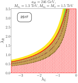
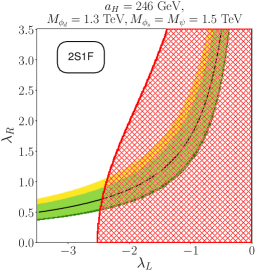
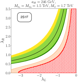
Figure 10: Results from Model 2S1F, scanning over the couplings of the new scalars and fermion to the left- and right-handed muon. The trilinear coupling which parametrises the mixing of the neutral BSM scalars is fixed to $a_{H}=246$ GeV. Colours are the same as in Fig. 9. In these scenarios the mass of either the scalar singlet $\phi_{s}$, scalar doublet $\phi_{d}$, or fermion $\psi_{s}$ is displaced by $200$ GeV from the other BSM masses at $1500$ GeV.

The situation can be changed substantially if we split the masses of the new states. The relic density of each point will in general be larger, since mass splittings will suppress several relic density depletion mechanisms such as coannihilation channels. Fig. 10 investigates this for three example cases. In each of the three panels the mass of the fermion singlet is $200$ GeV away from the dark matter scalar, which in turn is either singlet- or doublet-dominated or a mixture. All panels of Fig. 10 can be compared to the middle panel of Fig. 9, where all masses were equal to $1500$ GeV. The contribution to $a_{\mu}$ is similar in all cases, with slight changes of the required couplings depending on the increased/decreased masses.

The dark matter phenomenology changes more dramatically. Both the relic density and the direct detection constraints differ strongly between the panels of Fig. 10 and compared to the middle panel of Fig. 9. Specifically the direct detection constraint ruled out a full explanation of the relic density in the equal mass case of the middle panel of Fig. 9. The same still happens in the third panel of Fig. 10, where the scalar doublet and singlet masses are equal. The reason in all these cases is the doublet–singlet mixing and the unsuppressed coupling of dark matter to the Higgs boson via the doublet–singlet–Higgs coupling $a_{H}$. In contrast, as soon as the scalar doublet and singlet masses are different (left and middle panels of Fig. 10), the direct detection constraints are weakened, and as a result a full explanation of the observed relic density is viable.

In detail the left panel of Fig. 10 illustrates the case where the dark matter candidate is dominantly a scalar singlet with only about a $1\%$ admixture of doublet. The singlet mass is set $200$ GeV lighter than the scalar doublet and the fermion masses. The relic density is driven up compared to the middle panel of Fig. 9 since several dark matter depletion mechanisms are suppressed. Generally, the scalar singlet participates only in few interactions and mostly annihilates through t-channel exchange of the BSM fermion. Although the singlet couples to BSM fermions only through $\lambda_{R}$, in the cross-section for t-channel exchange of the muon, contributions that depend only on $\lambda_{L}$ (or only on $\lambda_{R}$) are suppressed by either $m_{\mu}^{2}/M_{F}^{2}$ or by the relative velocity in comparison to the contribution proportional to $\lambda_{L}^{2}\lambda_{R}^{2}$. This leads to the shape of the red line that can be seen in the plot, where it follows a similar trajectory to the $a_{\mu}$ contours, which is approximately a hyperbola.

Strikingly in the left panel of Fig. 10 we find that the red curve, where the observed relic density can be explained, and the black curve, where $\Delta a_{\mu}^{\text{2021}}$ can be explained are very close to each other and follow the same trajectory. However while a 1$\sigma$ explanation of $\Delta a_{\mu}^{\text{BNL}}$ could have been accommodated, the slightly higher couplings required to explain relic density measurements means that the over abundance of dark matter now rules out most of the parameter space where $\Delta a_{\mu}^{\text{2021}}$ (Eq. (7)) can be explained, except for a small slice of parameter space with $\lambda_{R}>2.5$. Nonetheless this could be changed with small adjustments to the mass splitting and in general it is possible to explain $\Delta a_{\mu}^{\text{2021}}$ and relic density at the same time. Explanations of $\Delta a_{\mu}^{\text{2021}}$ are possible for masses above $1$ TeV, as long as the product $\lambda_{L}\lambda_{R}a_{H}$ is sufficient.

In the middle panel of Fig. 10 we instead focus on doublet-dominated dark matter, by setting the scalar doublet mass $200$ GeV lighter than both the scalar singlet and fermion (and again compared to the middle panel of Fig. 9). The impact on $\Delta a_{\mu}$ is very similar to what happened in the left plot as expected from Eq. (42). However, the change in the behaviour of dark matter is very different. Now the dark matter candidate has generally many more interaction channels via the SU(2)_L gauge interactions of the doublet component. Hence the relative importance of the $\lambda_{L,R}$ parameters is reduced compared to the singlet-dominated case. Although not visible in the plot, the overall variation of the relic density is much reduced compared to the left panel or the middle panel of Fig. 9. The residual dependence on $\lambda_{L}$ is still important to deplete the relic density sufficiently, but the residual dependence on $\lambda_{R}$ via the singlet-admixture is of minor importance. In this case the constraints from the relic density and from $\Delta a_{\mu}$ are essentially orthogonal in the parameter space and thus complementary. Both constraints can be fulfilled, but agreement can only be achieved for very large values of $|\lambda_{L}|$ ($\approx$ between $2.4$ and $2.5$ when $\Delta a_{\mu}^{\text{2021}}$ is explained with $1\sigma$).

In the right panel of Fig. 10 we raise the fermion mass by $200$ GeV, compared to the middle panel of Fig. 9. Here we can see that this slightly increases the size of the couplings required to explain the measured $\Delta a_{\mu}$ values. As mentioned before, however, in this case with equal scalar singlet and doublet masses the relic density must be under abundant because of direct detection constraints. Raising the fermion mass suppresses the coannihilation mechanisms involving the fermion, which are strongly dependent on the couplings $\lambda_{L}$ and $\lambda_{R}$, but t-channel fermion exchange can still be active as suggested by the fact that the relic density curve is again a hyperbola similar to the left panel. However since the singlet and doublet masses are equal in this case, the usual $SU(2)$ scalar doublet (co)annihilations have greater impact, reducing the required size of $\lambda_{L}\lambda_{R}$. Due to the rescaling, the direct detection constraints reflect this behaviour. With the chosen value of $a_{H}=246$ GeV $\Delta a_{\mu}^{\text{2021}}$ can be explained with an under abundant relic density.

Just as for Fig. 9, we can change $a_{H}$ to see if we can simultaneously explain $a_{\mu}$ and dark matter. Currently in the middle panel of Fig. 10, as well as the left panel with very large $\lambda_{R}$, we can already explain $a_{\mu}^{\text{2021}}$ and dark matter simultaneously. As we saw previously increasing $a_{H}$ increases the constraints from direct detection. For the left panel as nearly all of the parameter space that can explain $\Delta a_{\mu}^{\text{2021}}$ to within $1\sigma$ is ruled out by over abundant dark matter, we can decrease $a_{H}$ to push the parameter space up into the under abundant regions. However, by increasing $a_{H}$ for the middle panel, the observed dark matter relic density line would become more dependent on $\lambda_{R}$, as the two scalars mix more. For the right panel, again increasing $a_{H}$ would cause the regions ruled out by direct detection to become more prevalent, while pulling the space which can explain $\Delta a_{\mu}^{\text{2021}}$ closer to it. However, while decreasing $a_{H}$ would shrink the regions constrained by direct detection, the red line does not shift close enough to the band which can explain $\Delta a_{\mu}^{\text{2021}}$, which itself would move away up and to the left as $a_{H}$ is decreased. So in the scenario with $M_{\psi}$ increased slightly from $M_{\phi_{s}}=M_{\phi_{d}}=1.5$ TeV, it is never possible to explain $\Delta a_{\mu}^{\text{2021}}$ and the dark matter relic density simultaneously, even if we adjust $a_{H}$.

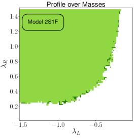
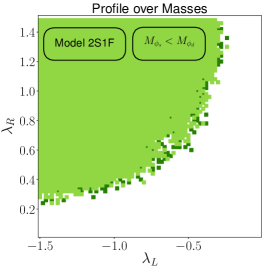
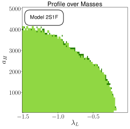
Figure 11: Profile over the $\lambda_{L}-\lambda_{R}$ plane or the $\lambda_{L}-a_{H}$ plane for Model 2S1F, scanning over the masses of the new scalars and fermion between $0$ and $5000$ GeV, as well as the mixing $a_{H}\leq 5000$ GeV and coupling $\lambda_{R}\in[0,1.5]$. Colours are the same as in Fig. 9. The scan targeted the observed value of the dark matter relic density $0.1200$, Eq. (8), the value of $\Delta a_{\mu}$ in Eq. (6), and the direct detection log likelihood provided by DDCalc [508, 509], where points which are excluded by direct detection or are more than $3\sigma$ away from the Planck observation are thrown away.

In all the two-dimensional slices of parameter space we presented, explaining $\Delta a_{\mu}^{\text{2021}}$ and dark matter is only possible with sizable interactions between the BSM states and muons, $\lambda_{L}$ and $\lambda_{R}$. Indeed the relic density is over abundant when both $\lambda_{L}$ and $\lambda_{R}$, are small because both the t-channel exchange of the BSM fermion and coannihilations with the BSM fermion are driven by these $\lambda_{L}$ and $\lambda_{R}$ couplings. At lighter masses both these processes and (co)annihilation processes involving $SU(2)$ interactions of the scalar doublet will become more efficient as the mass suppression is reduced, with the $SU(2)$ interactions becoming more significant relative to $\lambda_{L}$ and $\lambda_{R}$. These effects imply that at much lighter masses it should be possible to also deplete the relic density with much smaller $\lambda_{L}$ and $\lambda_{R}$. At the same time, explaining $\Delta a_{\mu}^{\text{BNL}}$ or $\Delta a_{\mu}^{\text{2021}}$ with smaller couplings is also possible when all the masses are small. However because it is possible for the observed relic density to be obtained through $SU(2)$ interactions of a $600$ GeV scalar doublet, it is not clear that with small couplings large $\Delta a_{\mu}$ and dark matter can be explained simultaneously as the $a_{\mu}$ explanation may then require larger values of $\lambda_{L}$ and $\lambda_{R}$ (or smaller masses) than what is required for fitting the relic density. Whether dark matter and the $a_{\mu}$ anomalies can be simultaneously explained for all $\lambda_{L}$, $\lambda_{R}$ or if there is a lower bound on these couplings just from these requirements remains an open question.

Therefore we now turn to a complete exploration of the parameter space of this model, varying $M_{\phi_{s}}$, $M_{\phi_{d}}$, $M_{\psi}$, $a_{H}$, $\lambda_{L}$, and $\lambda_{R}$ to see the impact of the new $\Delta a_{\mu}^{\text{2021}}$ measurements and address the question posed above. We vary $M_{i}\in[0,5000]$, $a_{H}\in[0,5000]$, $\lambda_{L,R}\in[0,1.5]$ in a number of MultiNest [495, 496, 497, 498] scans with a likelihood constructed to target $\Omega_{h^{2}}=0.1200$, different possible values of $a_{\mu}$ and solutions which evade direct detection limits. In total we collected about 15 million samples targeting several different values in the range $\Delta a_{\mu}\underset{\sim}{\in}[0,42\times 10^{-10}]$.

In the left panel of Fig. 11 we present results in the $\lambda_{L}$–$\lambda_{R}$ plane. This shows that it is only possible to explain the $a_{\mu}^{\text{BNL}}$ measurement and dark matter simultaneously when $|\lambda_{L}\lambda_{R}|\geq 0.22$. With the new $a_{\mu}^{\text{FNAL}}$ measurement this limit update changes very little. Couplings smaller than this cannot simultaneously explain $a_{\mu}^{\text{2021}}$ and dark matter. For the case of scalar doublet dominated dark matter the $SU(2)$ interactions will deplete the relic density to below the observed value whenever $m_{\phi_{d}}\lesssim 600$ GeV and this limit on the lightest mass makes explaining large $\Delta a_{\mu}$ impossible for such small couplings. For pure scalar singlet dark matter, note that if the scalar doublet is so heavy it completely decouples, then the model effectively reduces to that of Model R from the two field section. There we already found that a simultaneous explanation of dark matter and the $a_{\mu}$ measurements is only possible for very large $\lambda_{R}$ (higher than the values shown in Fig. 11) and not possible at all when collider limits are also taken into account.

If instead the dark matter has a significant admixture of both the scalar singlet and the scalar doublet, then the situation is a bit more complicated. With both singlet and doublet mixing, the relic density can deplete through processes involving both $\lambda_{L}$ and $\lambda_{R}$ couplings and $a_{H}$ in addition to the $SU(2)$ interactions of the doublet component. One can compensate increased splitting in the masses by raising $a_{H}$ to keep $\Delta a_{\mu}$ fixed to the measured value, or similarly one can reduce the mass splitting to compensate for reducing $a_{H}$ but in either case the relic density is still depleted too efficiently since both raising $a_{H}$ and reducing the mass splitting can enhance annihilation cross-sections. Increasing $a_{H}$ and reducing the mass splitting also increases direct detection cross-sections, increasing the tension with large $\Delta a_{\mu}$ further. Therefore when there is significant mixing between the scalar singlet and doublet, requiring that the measured relic density is obtained implies masses that are too large (for any given $a_{H}$ value) for large $\Delta a_{\mu}$ to be explained with small couplings. We also looked at scenarios where the dark matter is more singlet or more doublet in nature separately. We found quite similar limits on $\lambda_{L}\lambda_{R}$ emerge in both cases, though the more singlet DM case had a marginally higher limit, as can be seen in the middle panel of Fig. 11.

The tension with $a_{H}$ is also shown in the plot on the right panel of Fig. 11. There one can see that there is an upper limit on $a_{H}$, coming from the dark matter constraints discussed above. The value of $a_{H}$ can also be restricted by the need to avoid tachyonic scalars that would appear when $a_{H}v<M_{\phi_{s}}M_{\phi_{d}}$. However we find it is the limits from dark matter that leads to the constraint shown in the right panel of Fig. 11.

As a result we find a lower limit on $|\lambda_{L}\lambda_{R}|$ that increases with the value for $\Delta a_{\mu}$ used as a constraint. In this way we directly see the impact of the new $\Delta a_{\mu}^{\text{2021}}$ result on this model. We do not expect collider limits to affect our results here, since we do not find any solutions explaining both dark matter and $\Delta a_{\mu}^{\text{BNL}}$ or $\Delta a_{\mu}^{\text{2021}}$ where the lightest of the two scalar masses $M_{\phi^{0}_{1}}$ is below around $500$ GeV for our choice of coupling range ($\lambda_{L,R}\leq 1.5$). Our scan results also indicate interesting structure in the mass planes. We reserve the detailed discussion and presentation of such mass plane results for a future dedicated global fit of the model. Nonetheless it is clear from our results that the combination of parameters and masses that are allowed are significantly impacted by the interplay between dark matter and $a_{\mu}$ constraints. The $a_{\mu}^{\textrm{BNL}}$ and $a_{\mu}^{\textrm{FNAL}}$ measurements are therefore very important for the phenomenology of models like this and should be included in all such studies, and in any future global fits of any models like this.

5.2 Three-field model with two fermions, one charged scalar and fermionic dark matter

Having looked at scalar dark matter in the previous section we now consider a model with a fermionic dark matter candidate. For this we choose a minimal three-field model with two new fermions and one new scalar field, which we call Model 2F1S. Specifically this model extends the SM by adding three $\mathbb{Z}_{2}$-odd fields

$$\phi_{d}=\begin{pmatrix}\phi^{+}_{d}\\ \phi_{d}^{0}\end{pmatrix},~{} \psi_{d}=\begin{pmatrix}\psi^{0}_{d}\\ \psi_{d}^{-}\end{pmatrix},~{}\psi_{s}^{0}\,,$$ (44)

where $\phi_{d}$ is a scalar doublet with representation $({\bf{1}},{\bf{2}},\frac{1}{2})_{0}$, $\psi_{d}$ a Dirac fermion doublet with representation $({\bf{1}},{\bf{2}},-\frac{1}{2})_{1/2}$ expressed in Weyl spinors $\psi_{d}$ and its Dirac partner $\psi_{d}^{c}=(\psi_{d}^{0c\dagger},\psi_{d}^{-c\dagger})$, and $\psi_{s}^{0}$ a neutral singlet Weyl fermion with representation $({\bf{1}},{\bf{1}},0)_{1/2}$.

In principle the model allows scenarios with scalar dark matter, however we do not consider such scenarios here. We use the model as an illustration of fermionic dark matter, in which case the dark matter candidate is predicted to be a mixture of the fermion singlet and the neutral doublet component. Ref. [376] also studied the model in certain parameter slices. Here we intend to determine the full status of the model, studying the detailed parameter dependence and performing general scans of the parameter space.

The relevant interactions are:

$${\cal L}_{\text{2F1S}}=\bigg{(} \lambda_{1}H\cdot\psi_{d}\psi_{s}^{0}-\lambda_{2}\psi_{d}^{c}\psi_{s}^{0}H+\lambda_{L}L_{2}\cdot\phi_{d}\psi_{s}^{0}+\lambda_{R}\psi_{d}\mu\phi_{d}^{\dagger}$$

$$-M_{\psi_{d}}\psi_{d}^{c}\psi_{d}-\frac{M_{\psi_{s}}}{2}\psi_{s}^{0}\psi_{s}^{0}+h.c.\bigg{)}-M_{\phi}^{2}|\phi_{d}|^{2},$$ (45)

where the sign in front of the $\lambda_{2}$ term reflects our definition of $\psi_{d}^{c}$ as an $SU(2)$ anti-doublet.

The model has four new coupling parameters. $\lambda_{L,R}$ are the couplings to the left- and right-handed muon, similarly to the case of the previous Model 2S1F. The couplings $\lambda_{1,2}$ govern the mixing of the BSM fermions via the Higgs VEV, similarly to the $a_{H}$ parameter in the previous case. The products $\lambda_{i}\lambda_{L}\lambda_{R}$ are responsible for the new source of muon chirality flips (for $i=1,2$). To reiterate, this model can also be compared to the Bino-Higgsino-left smuon (BHL) system for the MSSM, see Eq. (62) below. There $\psi_{d}$ corresponds to the Higgsino, $\psi_{s}$ to the Bino, and $\phi_{d}$ to the left smuon doublet, and the couplings $\lambda_{1},\lambda_{2}$ and $\lambda_{L}$ would all correspond to the Bino coupling $g_{1}$, while $\lambda_{R}$ would correspond to the muon yukawa coupling. A difference is that the MSSM counterparts of the couplings $\lambda_{1,2}$ would couple the Higgsinos to the up-type and down-type Higgs doublets, and the resulting contributions to the mass mixings would involve the $\tan\beta$ parameter, while here there is just one single Higgs doublet and the mass mixing is simpler.

The mixing of the BSM fermions affects the singlet $\psi^{0}_{s}$ and the neutral components of the fermion doublet $\psi_{d}^{0}$ and its Dirac partner $\psi_{d}^{0c\dagger}$. They mix into three different flavours of neutral fermions $\psi^{0}_{i}$ with Majorana mass terms via the mixing matrix $V_{F}$:

$$\begin{split}{\cal L}_{\text{2F1S}}&\ni-\frac{1}{2}\begin{pmatrix}\psi_{s}^{0}&\psi_{d}^{0}&\psi_{d}^{0c\dagger}\end{pmatrix}\begin{pmatrix}M_{\psi_{s}}&\frac{\lambda_{1}v}{\sqrt{2}}&\frac{\lambda_{2}v}{\sqrt{2}}\\ \frac{\lambda_{1}v}{\sqrt{2}}&0&M_{\psi_{d}}\\ \frac{\lambda_{2}v}{\sqrt{2}}&M_{\psi_{d}}&0\end{pmatrix}\begin{pmatrix}\psi_{s}^{0}\\ \psi_{d}^{0}\\ \psi_{d}^{0c\dagger}\end{pmatrix}=-\frac{1}{2}\sum_{i=1,2,3}M_{\psi_{i}^{0}}\psi_{i}^{0}\psi_{i}^{0}\,,\end{split}$$ (46)

where

$$\begin{pmatrix}\psi_{1}^{0}\\ \psi_{2}^{0}\\ \psi_{3}^{0}\end{pmatrix}=V_{F}^{T}\begin{pmatrix}\psi_{s}^{0}\\ \psi_{d}^{0}\\ \psi_{d}^{0c\dagger}\end{pmatrix}\,.$$ (47)

The contribution to $a_{\mu}$ from this model comes from two diagrams, the FFS diagram of Fig. 19(a) and the SSF diagram of Fig. 19(b), with the generic $F$ fermion lines replaced by $\psi^{-}$ and $\psi_{i}^{0}$ and the scalar $S$ ones by $\phi^{0}_{d}$ and $\phi^{+*}_{d}$, respectively. Among these diagrams, only the SSF diagram with neutral fermion exchange can lead to an enhanced chirality flip. The full contributions are given by:

$$\Delta a_{\mu}^{\text{2F1S}}= \frac{m_{\mu}^{2}}{32\pi^{2}M_{\phi}^{2}}\bigg{(}\frac{\lambda_{R}^{2}}{6}\,E\!\begin{pmatrix}\frac{M^{2}_{\psi_{d}}}{M^{2}_{\phi}}\end{pmatrix}-\sum_{i=1}^{3}\frac{\lambda_{R}^{2}|V_{F\,2i}|^{2}+\lambda_{L}^{2}|V_{F\,1i}|^{2}}{6}\,B\!\begin{pmatrix}\frac{M^{2}_{\psi_{i}^{0}}}{M^{2}_{\phi}}\end{pmatrix}$$

$$+\sum_{i=1}^{3}\frac{M_{\psi_{i}^{0}}}{m_{\mu}}\frac{2\lambda_{L}\lambda_{R}V_{F\,1i}V_{F\,2i}}{3}\,C\!\begin{pmatrix}\frac{M^{2}_{\psi_{i}^{0}}}{M^{2}_{\phi}}\end{pmatrix}\bigg{)}.$$ (48)

The term in the second line corresponds to the additional source of chirality flip in the model. It can be analyzed similarly to the term in Eq. (42). The actual enhancement factor, beyond the loop and mass suppression factor, is given by the coupling combination $\lambda_{1,2}\lambda_{L}\lambda_{R}/y_{\mu}$ where the $\lambda_{1,2}$ are contained in the product of the mixing matrix elements $V_{F\,1j}V_{F\,2j}$ of the neutral fermions. If this coupling combination vanishes, the new chirality flip contribution and the third term disappear, and we end up with the contribution of Model L from Sec. 4, Eq. (34).

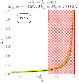
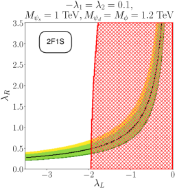
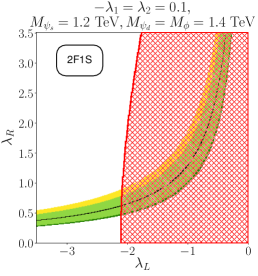
Figure 12: Results from Model 2F1S, scanning over the couplings of the new fermions and scalar to the left- and right-handed muon. Colours are the same as in Fig. 9. The mixing couplings are fixed to $-\lambda_{1}=\lambda_{2}=0.1$. In this scenario the masses of the scalar doublet $\phi_{d}$ and fermion doublet $\psi_{d}$ are raised by $200$ GeV above the mass of the fermion singlet $\psi_{S}$. Points to the right of the red line produce an over abundance of dark matter and are strongly excluded.

The case of a pure fermion $SU(2)$ doublet dark matter candidate is very well known as this corresponds to Higgsino dark matter in the MSSM, or the lowest representation of minimal dark matter [510]. In that case it is possible to deplete the relic density to the measured value, using only $SU(2)$ gauge interactions, when the fermion doublet has a mass of $1$ TeV [483] while above (below) it will be over (under) abundant. This can be adjusted by mixing with singlet, to obtain well-tempered dark matter[483] where the rapid depletion of dark matter from $SU(2)$ interactions are diluted through mixing with the singlet, though well-tempered dark matter is heavily constrained by direct detection (see e.g. Fig. 8 of Ref. [511]). As in the previous example explaining $\Delta a_{\mu}^{\text{BNL}}$ and $\Delta a_{\mu}^{\text{2021}}$ after including the FNAL result will require significant values of the $\lambda_{L}$, $\lambda_{R}$ and $\lambda_{i}$ couplings, leading to additional depletion mechanisms. Therefore scenarios where all the input masses are set to be equal will only explain dark matter at very heavy masses.

Instead we first focus on scenarios where the dark matter is dominantly singlet in nature in Fig. 12, showing two dimensional parameter slices in the $\lambda_{L}$–$\lambda_{R}$ plane, with the overall mass scale increasing between the panels from left to right. Specifically each of the three panels shows scenarios where the fermion doublet $\psi_{d}$ and scalar doublet $\phi_{d}$ are always $200$ GeV higher than the mass of the fermion singlet $\psi_{s}^{0}$. To simplify things further, we choose fairly small values for the mixing parameters $-\lambda_{1}=\lambda_{2}=0.1$, since large singlet–doublet mixing increases dark matter direct detection constraints and depletes the relic density. The other couplings are varied in the range $-\lambda_{L},\lambda_{R}\in[0,3.5]$.

As a function of $\lambda_{L},\lambda_{R}$, we get a similar curve for $a_{\mu}^{\text{2021}}$ to the ones shown in Figs. 9, 10, due to the dominant chirality flip contribution of Eq. (5.2) having the same dependence on $\lambda_{L}\lambda_{R}$ as Eq. (42). The nearly vertical red lines indicate points in agreement with the Planck observed [416] dark matter relic abundance; points to the right are over abundant and excluded. As can be seen in all panels of Fig. 12, all points allowed by the dark matter relic density are also in agreement with direct detection constraints due to the small values of the $\lambda_{i}$ coupling .

Going from left to right in the three panels of Fig. 12, the singlet mass is increased from $500$ GeV to $1000$ GeV and $1200$ GeV, while the mass splitting remains $200$ GeV. In the left panel the dark matter relic abundance depends only on $\lambda_{L}$, the coupling of the singlet to the muon and the BSM scalar, due to the large mixing suppression of any $\lambda_{R}$ contribution through the fermion doublet component of the dark matter. In the middle and right panels the relative doublet content of the dark matter candidate rises, opening up additional annihilation mechanisms through the $SU(2)$ interactions and the $\lambda_{R}$ coupling. Thus when $\lambda_{R}$ is large t-channel exchange of the BSM scalars may play a role through $\lambda_{R}$, leading to the curvature of the red line, which is most pronounced in the right panel. Therefore, while in the left panel avoiding an over abundance of dark matter gives a simple bound of $\lambda_{L}<-1.5$, in the middle and right panel larger values of $|\lambda_{L}|$ are required to deplete the relic density to the observed value or below, and the precise limit also depends on $\lambda_{R}$. In all panels $\Delta a_{\mu}^{\text{2021}}$ can be explained simultaneously with the relic density if $\lambda_{R}$ has the rather small values $\lambda_{R}\in[0.1,0.7]$.

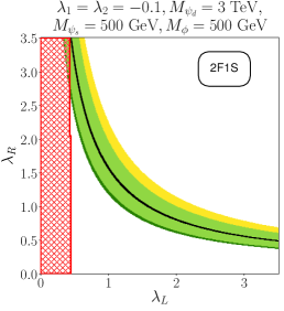
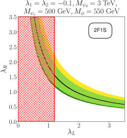
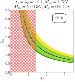
Figure 13: Results from Model 2F1S, scanning over the couplings of the new scalars and fermion to the left- and right-handed muon. Colours are the same as in Fig. 9. The mixing couplings are fixed to $\lambda_{1}=\lambda_{2}=-0.1$. In this scenario the fermion doublet has its mass fixed at $M_{\psi_{d}}=3000$ GeV, the fermion singlet is fixed at $M_{\psi_{s}}=500$ GeV, and the scalar doublet has its mass slowly increased from $M_{\psi_{s}}$. Points below or to the left of the red line produce an over abundance of dark matter and are strongly excluded.

The mass splitting between the singlet fermion $\psi_{s}$ and the scalar doublet $\phi$ has a large impact on the relic density. In Fig. 13 we show this impact by varying this mass splitting over three $\lambda_{L}$–$\lambda_{R}$ planes, specifically we fix $M_{\psi_{s}}=500$ GeV and set $M_{\phi}=500$ GeV, $550$ GeV and $600$ GeV in the left, middle and right panels respectively. At the same time we keep the fermion doublet mass fixed at a heavy scale $M_{\psi_{d}}=3000$ GeV, well above that of the dark matter candidate, so that in this case it will not play any role in the depletion of dark matter relic density. This choice also suppresses the $\Delta a_{\mu}$ prediction and means that very large couplings are required to explain $\Delta a_{\mu}^{\text{BNL}}$ and $\Delta a_{\mu}^{\text{2021}}$. We also choose $\lambda_{1,2}=-0.1$ and $\lambda_{L}>0$. The relative sign change between $\lambda_{1}$ and $\lambda_{2}$ leads to destructive interference between different terms and thus a further slight suppression of the overall contributions to $\Delta a_{\mu}$.

In all three panels of Fig. 13 the relic density depends only on $\lambda_{L}$ due to the decoupling of the doublet state, while $\Delta a_{\mu}$ depends on both $\lambda_{L}$ and $\lambda_{R}$ since the chirality flip enhancement is proportional to $\lambda_{L}\lambda_{R}$. Just as before, in all cases we can explain the discrepancy in $a_{\mu}$ and provide a dark matter candidate particle simultaneously. Between the three panels the $\Delta a_{\mu}$ result only changes a little, as expected due to the small mass increases. However the dark matter relic density depends strongly on the value of the mass splitting. In the left panel where $M_{\phi}=M_{\psi_{s}}$, most of the parameter space has an under abundance of dark matter. The very small mass splitting between the dark matter fermion $\psi_{1}^{0}$ and the BSM scalar opens up coannihilation channels which were suppressed in Fig. 12. Due to these highly efficient coannihilations the relic density is depleted for much smaller values of $\lambda_{L}$ than in the previous figures. When $M_{\phi}$ is increased to $550$ GeV in the middle panel, the (co)annihilations through $\lambda_{L}$ become less efficient. As a result a much larger $\lambda_{L}\approx 1.1$ is required to deplete the relic density to the observed value via t-channel processes as in the case of Fig. 12. Increasing the scalar mass further to $600$ GeV (right panel) an even larger $\lambda_{L}\approx 1.4$ is required to produce a relic abundance that matches the Planck observation. However while the bound from an over abundant relic density changed a lot between $500$ GeV and $550$ GeV, as we move away from the optimal window for coannihilations, subsequently increasing $M_{\phi}$ above $600$ GeV has a much weaker impact. If we increase the scalar mass further the relic density limit gradually increases until somewhere between $2.3$–$2.4$ TeV it is no longer possible to deplete the relic density to the observed value or below with perturbative couplings.

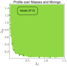
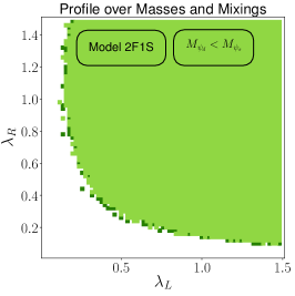
Figure 14: Viable points in the $\lambda_{L}-\lambda_{R}$ plane obtained from scanning over the masses of the new scalar and fermions between $0$ and $5000$ GeV, as well as the Yukawa couplings $\lambda_{L,R}\in[0,1.5]$ and $\lambda_{1,2}\in[0,3.5]$ for Model 2F1S. Colours are the same as in Fig. 9. Scan targeted the observed value of the dark matter relic density $0.1200$, Eq. (8), the $a_{\mu}$ value in Eq. (6), and the direct detection log likelihood provided by DDCalc [508], where points which are excluded by direct detection limits or are more than $3\sigma$ away from the Planck observation are thrown away.

In Sec. 5.1 the fact that a $600$ GeV scalar dark matter candidate naturally depletes the relic density to the observed value played a critical role in leading to a lower bound on $|\lambda_{L}\lambda_{R}|$ from the combination of $\Delta a_{\mu}$ and dark matter constraints. Since a pure fermion doublet naturally depletes the relic density to the observed value when it has a mass of about $1.1$ TeV, we may anticipate a similar result in this model. In addition we have also seen that when the doublet fermion is very heavy, large couplings are required, while mixed singlet-doublet fermion dark matter scenarios should be strongly constrained by direct detection. Therefore we now perform a scan over the full parameter space of the Model 2F1S to see if this also leads to a lower bound on $|\lambda_{L}\lambda_{R}|$.

We sample all free parameters in this model ($\lambda_{1},\lambda_{2},\lambda_{L}$, $\lambda_{R}$, $M_{\phi}$, $M_{\psi_{d}}$, and $M_{\psi_{s}}$) using MultiNest [495, 496, 497, 498], with mass range $M_{i}\in[0,5000]$ GeV, and the BSM Yukawa couplings having the values $\lambda_{L,R}\in[0,1.5]$ and $\lambda_{1,2}\in[0,3.5]$, with the results shown in Fig. 14. Again, several values of $\Delta a_{\mu}$ where targeted in the range $[0,42]\times 10^{-10}$, with a total of 62 million points scanned. In the left panel of the figure, we can see that there is a lower bound on the couplings $|\lambda_{L}\lambda_{R}|\gtrsim 0.036$ below which we cannot simultaneously explain the measured value of $a_{\mu}$ whilst producing a dark matter candidate particle with the observed relic density that escapes direct detection limits. As we anticipated in the discussion above, pure singlet fermion dark matter requires larger couplings to explain large $\Delta a_{\mu}$, while fermion doublet dark matter annihilates too effectively for light masses.

Significant singlet-doublet fermion mixing can dilute the $SU(2)$ gauge interactions of the doublet, but does not avoid this problem as it means that t-channel exchange of the BSM scalars will be active through both $\lambda_{L}$ and $\lambda_{R}$, and increasing the mixing also increases direct detection. Reducing $\lambda_{L}\lambda_{R}$ while increasing $\lambda_{i}$ to keep the $\Delta a_{\mu}$ prediction fixed makes direct detection limits more relevant. As a result the combination of these constraints leads to the lower limit $|\lambda_{L}\lambda_{R}|$ shown in the plot. Interestingly we also find a more severe limit on $|\lambda_{L}\lambda_{R}|\approx 0.14$ for dark matter that is mostly doublet in nature, as shown in the right panel of Fig. 14.

As in the previous case this shows how the $a_{\mu}$ measurements have have a significant impact on the model, implying a siginifcant constraint on the couplings. However since the new world average is quite close to the BNL value there is little difference between the limits implied by the $\Delta a_{\mu}^{\text{BNL}}$ and $\Delta a_{\mu}^{\text{2021}}$ results. The masses in our samples are mostly heavy enough to easily evade collider limits. However collider limits should be included in a full global fit of the model, but we leave that and a presentation of the full impact of all constraints on all parameters and masses to future work. Again we stress that our results demonstrate that the FNAL measurement plays a critical role in the phenomenology of these models and should be included in all phenomenological studies of models of this type and future global fits.

As discussed earlier this model can be compared to the BHL scenario of the MSSM. There since $\lambda_{L}\lambda_{R}\lambda_{i}$ corresponds to $g_{1}^{2}y_{\mu}$, $a_{\mu}$ can only be explained with masses less than $200$ GeV, due to the weaker enhancement [217]. Similarly the $|\lambda_{L}\lambda_{R}|$ bound corresponds to $g_{1}y_{\mu}$, which should be well below the bound for this model and would suggest that the BHL scenario alone cannot explain both the measured $a_{\mu}$ and dark matter. However it is important to note that the comparison is not perfect due to the fact that the MSSM contains two Higgs doublets, which gives an additional enhancement from the ratio of the two Higgs VEVs, $\tan\beta$. As a result in the BHL scenario, a dominantly bino dark matter candidate can simultaneously explain dark matter and account for $\Delta a_{\mu}^{\text{BNL}}$ and $\Delta a_{\mu}^{\text{2021}}$ despite having couplings below the lower bound for this in the Model 2F1S. On the other hand, the Model 2F1S has much greater freedom to explain dark matter and large $\Delta a_{\mu}$ at much higher masses than is possible in the BHL scenario. The fact that the $\lambda_{R}\neq y_{\mu}$ in this model is of great significance, but on top of that the freedom to push all couplings up to values much larger than that of $g_{1}$ and to vary the interactions independently, gives rise to a rich and distinct phenomenology.

Therefore our results show that this class of simple models provide an interesting way to explain both dark matter and large $\Delta a_{\mu}$. They are complementary to the explanations that come from the MSSM and appear to be significantly less constrained. However these models have not been constructed from any principle other than to explain the phenomenology, and as a result the deeper motivation is unclear. It would be very interesting to consider whether models that are motivated from more fundamental principles can have such scenarios as a low energy effective field theory.

6 Supersymmetry and the Minimal Supersymmetric Standard Model

In the present section we consider the Minimal Supersymmetric Standard Model (MSSM). It is one of the most promising extensions of the SM and offers potential explanations of EW naturalness and of dark matter as the lightest supersymmetric particle (LSP), it is compatible with unification of gauge couplings — and it could easily explain the deviation $\Delta a_{\mu}$ based on the initial BNL measurement. However a tension has developed because of LHC and dark matter searches, which severely constrain the MSSM parameter space. The tension remains in place in view of the new FNAL result (1) if the MSSM is required to accommodate the deviation $\Delta a_{\mu}^{\text{2021}}$.

Here we present an update and investigate the parameter space of the MSSM which can accommodate this deviation, given the new FNAL measurement Eq.  (1) and the SM theory update (4). We focus particularly on the combined constraints from LHC and dark matter direct detection (DMDD) searches.

The MSSM contributions have been extensively studied in the past. For analyses and reviews of the basic behaviour we refer to Refs. [512, 74, 49, 166]; higher-precision calculations were done in Refs. [87, 86, 159, 160, 161, 162, 163, 164, 165]. For recent studies in the light of LHC run-II data we refer to Refs. [201, 200, 202, 203, 204] (which involve a detailed recasting of LHC data) and [205, 206, 207, 213, 216, 217, 215, 209, 210, 218, 214, 208, 211, 212, 223, 222, 224, 220, 221, 219, 228, 225, 227, 226, 230, 229, 231, 232, 233, 234, 235, 236] (which involve model building, the construction of specific scenarios and/or constraints from dark matter or electroweak precision observables). Earlier studies of the SUSY phenomenology of $a_{\mu}$ of the LHC run 1 era can be found in Refs. [166, 167, 169, 168, 171, 170, 175, 177, 174, 178, 173, 176, 172, 179, 180, 182, 181, 186, 190, 183, 189, 192, 193, 187, 191, 184, 185, 188, 195, 196, 194, 197, 198, 199]. Refs. [334, 336] study simultaneous SUSY explanations of $(g-2)$ of both the muon and the electron. We will provide more detailed comparisons to the literature in the following subsections.

The MSSM contributions to $a_{\mu}$ are mainly generated by left- and right-handed smuons ${\tilde{\mu}}_{\text{L},\text{R}}$, sneutrino ${\tilde{\nu}}_{\mu\text{L}}$, Bino ${\tilde{B}}$, Winos ${\tilde{W}}_{1,2,3}$, and Higgsinos ${\tilde{H}}_{u,d}$ which are the SUSY partners of the muon, muon-neutrino, and the electroweak SM gauge and Higgs bosons. ${\tilde{B}}$, ${\tilde{W}}_{1,2,3}$ and ${\tilde{H}}_{u,d}$ form neutralinos $\chi^{0}_{1,2,3,4}$ and charginos $\chi^{\pm}_{1,2}$ mass eigenstates. They appear in the one-loop diagrams of Fig. 19(a) (with charginos and sneutrinos) and of Fig. 19(b) (with neutralinos and smuons).

To provide a brief overview and set the stage for the following discussion we present Fig. 15 and the following approximation of the leading MSSM contributions to $a_{\mu}$,

$$\Delta a_{\mu}^{1{\rm L}}(\text{WHL}) \approx 21\times 10^{-10}\text{sign}(\mu M_{2})\left(\frac{500\text{ GeV}}{M_{\text{SUSY}}}\right)^{2}\frac{\tan\beta}{40},$$ (49a)

$$\Delta a_{\mu}^{1{\rm L}}(\text{BHL}) \approx 1.2\times 10^{-10}\text{sign}(\mu M_{1})\left(\frac{500\text{ GeV}}{M_{\text{SUSY}}}\right)^{2}\frac{\tan\beta}{40},$$ (49b)

$$\Delta a_{\mu}^{1{\rm L}}(\text{BHR}) \approx-2.4\times 10^{-10}\text{sign}(\mu M_{1})\left(\frac{500\text{ GeV}}{M_{\text{SUSY}}}\right)^{2}\frac{\tan\beta}{40},$$ (49c)

$$\Delta a_{\mu}^{1{\rm L}}(\text{BLR}) \approx 2.4\times 10^{-10}\text{sign}(\mu M_{1})\left(\frac{500\text{ GeV}}{M_{\text{SUSY}}}\right)^{2}\frac{\tan\beta}{40}\frac{\mu}{500\text{ GeV}}.$$ (49d)

The letters B,W,H,L, and R are the abbreviations for Bino, Winos, Higgsinos, and Left-and Right-handed smuons respectively. As indicated by the letters in brackets, each contribution depends on three of these states and their respective masses. In each formula the three appropriate masses have been set to a common scale $M_{\text{SUSY}}$ and $M_{\text{SUSY}}\gg M_{Z}$ is assumed. The approximations highlight the linearity in $\tan\beta=v_{u}/v_{d}$, the ratio of the two MSSM Higgs VEVs.

The physics of the individual contributions is as follows. In the first three lines the muon chirality is flipped at the Yukawa coupling to a Higgsino; the Higgsino is then converted to a gaugino via a Higgs vacuum expectation value. The appearance of the enhanced VEV is always accompanied by a factor of the Higgsino mass $\mu$. This explains the appearance of one Higgsino, one gaugino (Bino or Wino) and of the factors $\tan\beta$ and $\mu$ in the numerators.

The BLR contribution in the fourth line is special. Here the muon chirality is flipped at the smuon line via the insertion of a smuon-left-right flip, which is governed by a product of the Higgsino mass $\mu$ and the enhanced VEV in the smuon mixing matrix. This explains the appearance of left- and right-handed smuons and of the factors $\tan\beta$ and $\mu$ in the numerator. In contrast to the other contributions, the BLR contribution is approximately linearly enhanced by the Higgsino mass $\mu$ since this parameter does not appear as the mass of a virtual Higgsino. The signs of all contributions are determined by the signs of $\mu$ and the gaugino masses $M_{1,2}$. In the following we will only consider positive signs of all these parameters, leading to positive MSSM contributions to $a_{\mu}$.

Figure 15 shows the theoretical maximum of the SUSY contributions (i.e. MSSM minus SM contributions) $a_{\mu}^{\text{SUSY,Max}}$ in the plane of $m_{\chi^{\pm}_{2}}$ and $m_{{\tilde{\mu}}_{1}}$, where $\chi^{\pm}_{2}$ is the heavier chargino and $\tilde{\mu}_{1}$ the lighter smuon (for similar plots in different planes see Refs. [139, 49, 182]). It fixes $\tan\beta=40$ and allows all SUSY masses to vary independently between $100$ GeV and 4 TeV, for further details see the caption. The red dashed lines and the yellow/green coloured regions correspond to the indicated values of $a_{\mu}^{\text{SUSY,Max}}$; specifically the yellow and green colours correspond to the $1\sigma$ regions for the BNL deviation and the new deviation including FNAL in Eqs. (6,7), respectively; the bright green colour corresponds to the overlap region. As indicated on the right of the legend plot, an alternative interpretation of the contour lines and regions is possible. Thanks to the approximate linearity in $\tan\beta$, each value for $a_{\mu}^{\text{SUSY}}$ with $\tan\beta=40$ can be translated into approximate $\tan\beta$-values for which the other values of $a_{\mu}^{\text{SUSY}}$ can be obtained. In the legend plot this translation is done for $\Delta a_{\mu}^{\text{2021}}={\color[rgb]{0,0,0}25.1\times 10^{-10}}$, the new experimental average deviation from the SM. E.g. on the contour labeled “20” we have $a_{\mu}^{\text{SUSY,Max}}=20\times 10^{-10}$ for $\tan\beta=40$, and equivalently we would get $a_{\mu}^{\text{SUSY,Max}}=\Delta a_{\mu}^{\text{2021}}$ for $\tan\beta\approx{\color[rgb]{0,0,0}50}$. On the contour labeled “50”, we have $a_{\mu}^{\text{SUSY,Max}}={\color[rgb]{0,0,0}50}\times 10^{-10}$ for $\tan\beta=40$, and the world average deviation can be explained for $\tan\beta\approx{\color[rgb]{0,0,0}20}$.

The figure and the formulas show that large contributions in the ballpark of the BNL deviation are of course possible but require upper limits on the SUSY masses. E.g. $a_{\mu}^{\text{SUSY}}>20\times 10^{-10}$ (which is just at the lower $1\sigma$ level of the deviation) can only be explained (for $\tan\beta=40$ and $\mu\leq 4$ TeV) if

• either both chargino masses are lighter than around 1.1 TeV (vertical black line in Fig. 15)

• or one smuon is lighter than around 700 GeV (horizontal black line in Fig. 15).

This already illustrates the potential tension between $a_{\mu}$ and LHC data since the LHC-searches are sensitive to chargino and smuon masses above these values. In addition to LHC, constraints from dark matter searches enforce lower limits on combinations of the chargino and neutralino masses. In more detail, the WHL contributions (49a) are by far most important in the largest part of parameter space. However for large $\mu$, the BLR contribution can become sizable as well. In Fig. 15 the slight rise of $a_{\mu}^{\text{SUSY,Max}}$ with increasing $m_{\chi^{\pm}_{2}}$ is due to the BLR contribution. In contrast, the BHR and particularly the BHL contributions are not important for the maximum value $a_{\mu}^{\text{SUSY,Max}}$, and in general they are practically always strongly suppressed, unless there are extremely large mass splittings between left- and right-handed smuons. We do not consider such cases in the present paper; hence in the following only the WHL and BLR contributions are important.

In the following subsections we will first introduce the SUSY contributions to $a_{\mu}$ in more detail (Sec. 6.1), survey relevant LHC and dark matter constraints (Sec. 6.2) and present a detailed phenomenological analysis and brief summary (Secs. 6.3, 6.4 and Sec. 6.5).

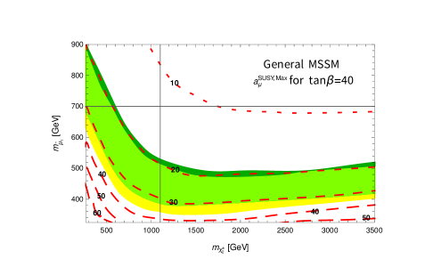
Figure 15: The theoretical maximum MSSM contribution $a_{\mu}^{\text{SUSY,Max}}$ for $\tan\beta=40$ in the plane of the heaviest chargino and the lightest smuon mass. (For each point in the plane, the actual value of the MSSM contribution can take any value between $0$ and $\pm a_{\mu}^{\text{SUSY,Max}}$, depending on the signs of parameters and details such as other masses and mixings.) The yellow/green coloured regions show where $a_{\mu}^{\text{SUSY,Max}}$ (for $\tan\beta=40$) is within the $1\sigma$ bands corresponding to the BNL and new deviations $\Delta a_{\mu}^{\textrm{BNL}}$ and $\Delta a_{\mu}^{\text{2021}}$, see Eqs. (6,7), and their overlap. The red dashed contour lines can be interpreted in two ways. Firstly, they directly correspond to certain values of $a_{\mu}^{\text{SUSY,Max}}$ for $\tan\beta=40$, as indicated in the left axis of the legend plot. Secondly, thanks to the approximate linearity in $\tan\beta$, each contour can be used to estimate the required $\tan\beta$ value for which $a_{\mu}^{\text{SUSY,Max}}$ agrees with the deviation $\Delta a_{\mu}^{\text{2021}}$ (keeping other input parameters fixed). These $\tan\beta$ values can be read off from the right axis of the legend plot (the values are approximate since the linearity is not exact). As an example of the reinterpretation we take the point $m_{\chi^{\pm}_{2}}=1750$ GeV and $m_{\tilde{\mu}_{1}}=700$ GeV. For $\tan\beta=40$ we get $a_{\mu}^{\text{SUSY,Max}}=10\times 10^{-10}$. The required $\tan\beta$ value to get $\Delta a_{\mu}^{\text{2021}}$ would be around 100, as read off from the right axis. The results for $a_{\mu}^{\text{SUSY,Max}}$ were obtained from a scan using GM2Calc [45] in which all relevant SUSY masses are varied independently between $100$ GeV and 4 TeV. The black lines indicate the maximum LHC reach for charginos and sleptons of $1100$ and $700$ GeV reported in Refs. [487, 490], respectively.

6.1 SUSY parameters and contributions to $a_{\mu}$

In the following we define our notation and provide details on the MSSM contributions to $a_{\mu}$. Our notation is essentially the same as e.g. in Refs. [74, 49, 166]. To fix it we provide the mass matrices of the charginos and neutralinos and the smuons:

$$X =\left(\begin{array}[]{cc}M_{2}&M_{W}\sqrt{2}\sin\beta\\ M_{W}\sqrt{2}\cos\beta&\mu\end{array}\right),$$ (52)

$$Y =\left(\begin{array}[]{cccc}M_{1}&0&-M_{Z}s_{\text{W}}\cos\beta&M_{Z}s_{\text{W}}\sin\beta\\ 0&M_{2}&M_{Z}c_{\text{W}}\cos\beta&-M_{Z}c_{\text{W}}\sin\beta\\ -M_{Z}s_{\text{W}}\cos\beta&M_{Z}c_{\text{W}}\cos\beta&0&-\mu\\ M_{Z}s_{\text{W}}\sin\beta&-M_{Z}c_{\text{W}}\sin\beta&-\mu&0\end{array}\right),$$ (57)

$$M_{\tilde{\mu}}^{2} =\left(\begin{array}[]{lr}m_{\mu}^{2}+m_{\text{L}}^{2}+M_{Z}^{2}\cos 2\beta\left(-\frac{1}{2}+s_{\text{W}}^{2}\right)&m_{\mu}(-\mu\tan\beta+A_{\mu}^{*})\\ m_{\mu}(-\mu^{*}\tan\beta+A_{\mu})&m_{\mu}^{2}+m_{\text{R}}^{2}+M_{Z}^{2}\cos 2\beta\ (-s_{\text{W}}^{2})\end{array}\right),$$ (60)

where the fundamental SUSY parameters appearing in these expressions are $\tan\beta$ and the two gaugino (Bino and Wino) mass parameters $M_{1,2}$, the Higgsino mass $\mu$ and the left-/right-handed smuon masses $m_{\text{L},\text{R}}$. The smuon mass matrix also involves the trilinear soft SUSY-breaking parameter $A_{\mu}$, which however will not play any role in the present paper. The other appearing parameters are the SM parameters $m_{\mu},M_{W,Z}$ and $s_{\text{W}}=\sqrt{1-c_{\text{W}}^{2}}$. In our numerical treatment the fundamental SUSY parameters are defined as running $\overline{\text{DR}}$-parameters at the scale 1 TeV, and the MSSMEFTHiggs_mAmu spectrum generator, created with FlexibleSUSY [43, 44] and incorporated in GAMBIT-1.3, is used for the precise evaluation of the spectrum of mass eigenvalues including higher-order corrections.

The 1-loop contributions of the MSSM to $a_{\mu}$ have been systematically and comprehensively studied in Ref. [512], for reviews see Refs. [74, 49, 166]. A wide range of higher-precision calculations of 2-loop contributions is available. Including higher-order corrections, the full known SUSY contributions (i.e. the difference between MSSM and SM contributions) to $a_{\mu}$ can be written as

$$a_{\mu}^{\text{SUSY}} =\left[a_{\mu}^{\rm 1L\,SUSY}+a_{\mu}^{\rm 2L(a)}+a_{\mu}^{\rm 2L,\ photonic}+a_{\mu}^{{\rm 2L,}f\tilde{f}}\right]_{t_{\beta}\text{-resummed}}\ ,$$ (61)

Refs. [87, 86, 159, 160, 154] evaluated all 2-loop diagrams $a_{\mu}^{\rm 2L(a)}$ in which a SUSY loop is inserted into a SM-like loop, including so-called Barr-Zee diagrams. Given current experimental constraints these diagrams are very small. Refs. [450, 163] computed leading QED-logarithms and the full 2-loop QED corrections $a_{\mu}^{\rm 2L,\ photonic}$; Refs. [162, 186] showed how to take into account $n$-loop higher-order terms enhanced by $(\tan\beta)^{n}$, i.e. carry out a $\tan\beta$-resummation. Finally Refs. [164, 165] computed genuine SUSY 2-loop corrections $a_{\mu}^{{\rm 2L,}f\tilde{f}}$ to the SUSY 1-loop diagrams which include non-decoupling effects from e.g. heavy squarks. Each of these three kinds of corrections can shift the 1-loop contributions by around 10%. All mentioned 1-loop and 2-loop contributions in Eq. (61) are implemented in the code GM2Calc [45], which is used in our later phenomenological evaluations.

The exact one-loop expression for $a_{\mu}^{\text{1L SUSY}}$ can be found in most mentioned references; a full overview of all contributions including higher orders is given in Ref. [45]. Here we provide the 1-loop contributions in mass-insertion approximation, which allows to directly read off the main parameter dependences. Following the form given e.g. in Refs. [166, 165, 186] they read

$$a_{\mu}^{\text{1L SUSY}} \approx\Delta a_{\mu}^{1{\rm L}}(\text{WHL})+\Delta a_{\mu}^{1{\rm L}}(\text{BHL})+\Delta a_{\mu}^{1{\rm L}}(\text{BHR})+\Delta a_{\mu}^{1{\rm L}}(\text{BLR}),$$

with

$$\Delta a_{\mu}^{1{\rm L}}(\text{WHL}) =\frac{g_{2}^{2}}{8\pi^{2}}\frac{m_{\mu}^{2}M_{2}}{m_{\text{L}}^{4}}\,\mu\tan\beta\,F_{a}\left(\frac{M_{2}^{2}}{m_{\text{L}}^{2}},\frac{\mu^{2}}{m_{\text{L}}^{2}}\right)$$

$$-\frac{g_{2}^{2}}{16\pi^{2}}\frac{m_{\mu}^{2}M_{2}}{m_{\text{L}}^{4}}\,\mu\tan\beta\,F_{b}\left(\frac{M_{2}^{2}}{m_{\text{L}}^{2}},\frac{\mu^{2}}{m_{\text{L}}^{2}}\right),$$ (62a)

$$\Delta a_{\mu}^{1{\rm L}}(\text{BHL}) =\frac{g_{1}^{2}}{16\pi^{2}}\frac{m_{\mu}^{2}M_{1}}{m_{\text{L}}^{4}}\,\mu\tan\beta\,F_{b}\left(\frac{M_{1}^{2}}{m_{\text{L}}^{2}},\frac{\mu^{2}}{m_{\text{L}}^{2}}\right),$$ (62b)

$$\Delta a_{\mu}^{1{\rm L}}(\text{BHR}) =-\frac{g_{1}^{2}}{8\pi^{2}}\frac{m_{\mu}^{2}M_{1}}{m_{\text{R}}^{4}}\,\mu\tan\beta\,F_{b}\left(\frac{M_{1}^{2}}{m_{\text{R}}^{2}},\frac{\mu^{2}}{m_{\text{R}}^{2}}\right),$$ (62c)

$$\Delta a_{\mu}^{1{\rm L}}(\text{BLR}) =\frac{g_{1}^{2}}{8\pi^{2}}\frac{m_{\mu}^{2}}{M_{1}^{3}}\,\mu\tan\beta\,F_{b}\left(\frac{m_{\text{L}}^{2}}{M_{1}^{2}},\frac{m_{\text{R}}^{2}}{M_{1}^{2}}\right).$$ (62d)

For SUSY masses significantly above $M_{Z}$ this is a very good approximation (of the 1-loop contributions). Physics explanations and numerical examples have already been given around Eq. (49). Next to $\tan\beta$ and the $SU(2)\times U(1)$ gauge couplings $g_{1,2}$, these contributions depend on the five independent SUSY mass parameters $M_{1,2}$, $\mu$ and $m_{\text{L},\text{R}}$ introduced above. The appearing loop functions are normalized as $F_{a}(1,1)=1/4$, $F_{b}(1,1)=1/12$ and can be found in the mentioned references as well as in Appendix A.

The linear enhancement in $\tan\beta$ already explained in Sec. 2 is apparent. The $\tan\beta$ enhancement is accompanied by explicit factors of the Majorana gaugino masses $M_{1,2}$ and the MSSM Higgsino mass parameter $\mu$.

As indicated, all contributions in Eq. (62) involve three different SUSY masses; the generic behaviour is $\propto 1/M_{\text{SUSY}}^{2}$. The BLR-contribution in Eq. (62) is special because it is linearly enhanced by large $\mu$; this enhancement arises via the smuon mixing off-diagonal element in Eq. (60).

Specific constraints on this BLR-contribution have been very thoroughly investigated in Ref. [176]. Most importantly, vacuum stability requires that staus, the superpartners of $\tau$-leptons, do not receive a charge-breaking vacuum expectation value, and this provides a constraint on the relation between the off-diagonal and diagonal elements of the stau mass matrix similar to Eq. (60). As a quantitative example, Ref. [176] finds that in case of universal left- and right-handed stau masses, the Higgsino mass has an upper limit, specifically

$$m_{\tilde{\tau}_{\text{L}}}=m_{\tilde{\tau}_{\text{R}}} =300\text{ GeV (}600\text{ GeV)} \Rightarrow \text{ }\mu \lesssim 1\text{ TeV (}2\text{ TeV)}\,.$$ (63)

In our later plots we will show the appropriate constraint in the approximate form of Eq. (14) of Ref. [176].

6.2 LHC and dark matter constraints on explanations of $\Delta a_{\mu}^{\text{2021}}$

Our aim is to analyze MSSM contributions to $a_{\mu}$ in the context of constraints from LHC and dark matter searches. Here we list the relevant constraints.

The relevant LHC constraints can be grouped into “standard” searches for electroweak particles (charginos/neutralinos and sleptons) and searches optimized for compressed spectra. The relevant searches are the following:

• Chargino/neutralino searches with decay into sleptons: The strongest chargino/neutralino mass limits are obtained from the pair production channel $pp\to{\chi}^{\pm}_{1}{\chi}^{0}_{2}$ with subsequent decay via on-shell sleptons into three charged leptons and two LSPs. In simplified-model interpretations, in which 100% decay branching ratios are assumed and the slepton mass is halfway between the LSP- and the chargino mass, the limits extend up to [487, 520]

  Chargino/slepton channel: $$\chi_{1}^{\pm}\chi_{2}^{0}\to\tilde{l}_{\text{L}}\nu\tilde{l}_{\text{L}}l(\tilde{\nu}\nu),l\tilde{\nu}\tilde{l}_{\text{L}}l(\tilde{\nu}\nu)\to l\nu\chi_{1}^{0},ll(\nu\nu)\chi_{1}^{0}$$ (64a)

  $$m_{\chi^{\pm}_{1}} \approx 1100\text{ GeV} (\text{for $m_{\text{LSP}}\approx 0\ldots 500\text{ GeV}$}),$$ (64b)

  $$m_{\text{LSP}} \approx 700\text{ GeV} (\text{for $m_{\chi^{\pm}_{1}}\approx 900\ldots 1000\text{ GeV}$}).$$ (64c)

  Further important, slightly weaker limits are obtained from the pair production channel $pp\rightarrow{\chi}^{\pm}_{1}{\chi}^{\mp}_{1}$ with subsequent decay via on-shell sleptons into two charged leptons and two LSPs. The limits in simplified-model interpretations reach up to $m_{\chi^{\pm}_{1}}\approx 1000$ GeV [490]. All limits of this kind depend on a significant mass splitting $\gtrsim 100$ GeV between the chargino and LSP masses; for smaller mass splittings the limits become much weaker.

• Chargino/neutralino searches with decay into other particles: The above limits are absent if the charginos cannot decay into sleptons e.g. because sleptons are too heavy. In such cases further limits are applicable. One such limit is obtained from the channel $pp\to{\chi}^{\pm}_{1}{\chi}^{0}_{2}$ assuming subsequent decays into on-shell $W$ and Higgs bosons plus LSP. This limit extends up to [521]

  Chargino/$$Wh \chi_{1}^{\pm}\chi_{2}^{0}\to Wh\chi_{1}^{0}\chi_{1}^{0},W\to l\nu,h\to b\bar{b}$$-channel: (65a)

  $$m_{\chi^{\pm}_{1}} \approx 750\text{ GeV} (\text{for $m_{\text{LSP}}\approx 0\ldots 100\text{ GeV}$}),$$ (65b)

  $$m_{\text{LSP}} \approx 250\text{ GeV} (\text{for $m_{\chi^{\pm}_{1}}\approx 600\text{ GeV}$}),$$ (65c)

  where Wino-like charginos and Bino-like LSP are assumed. If this assumption is not met, the production cross section is lower and/or the decay branching ratios are reduced [522]. Similar but slightly weaker limits are obtained in Ref. [523]. A complementary limit is obtained in Ref. [524] which searched for $pp\to{\chi}^{\pm}_{1}{\chi}^{\mp}_{1},{\chi}^{\pm}_{1}{\chi}^{0}_{2}$ with subsequent decays via $\tilde{\tau}$-sleptons (staus) into $\tau$-leptons. The limit in a simplified-model interpretation assuming Wino-like chargino reaches up to

  Chargino/stau-channel: $$\chi_{1}^{\pm}\chi_{2}^{0}\to\tilde{\tau}\nu\tilde{\tau}\tau(\tilde{\nu}\nu),\tau\tilde{\nu}\tilde{\tau}\tau(\tilde{\nu}\nu)\to\tau\nu\chi_{1}^{0},\tau\tau(\nu\nu)\chi_{1}^{0},$$ (66a)

  (66b)

  $$m_{\chi^{\pm}_{1}} \approx 760\text{ GeV} (\text{for $m_{\text{LSP}}\approx 0\ldots 200\text{ GeV}$}),$$ (66c)

  $$m_{\text{LSP}} \approx 300\text{ GeV} (\text{for $m_{\chi^{\pm}_{1}}\approx 600\ldots 700\text{ GeV}$}).$$ (66d)

  Figure 8 of Ref. [524] and the recasting study of Ref. [201] show that the limit is rather robust against changes of the stau masses and mixings and against the Higgsino content of the chargino. There exist further chargino searches with decays into $W$ and $Z$ bosons [487, 525, 490, 526, 527], however the resulting limits are weaker and do not lead to excluded regions of the parameter spaces we will consider.

• Slepton searches: Searches for the direct production of slepton pairs $\tilde{l}\tilde{l},(\tilde{l}=\tilde{e},\,\tilde{\mu})$ with subsequent decay into leptons plus LSP have been analyzed in Ref. [490] (based on $139\text{\,fb}^{-1}$ data) and [487, 488] (based on $36\text{\,fb}^{-1}$ data). The limits extend up to

  $$\text{Slepton \cite[cite]{[\@@bibref{}{Aad:2019vnb}{}{}]}}:\quad\parbox{0.0pt}{\mbox{$\tilde{l}_{\text{L},\text{R}}\tilde{l}_{\text{L},\text{R}}\to l^{+}l^{-}\chi_{1}^{0}\chi_{1}^{0},$}}$$ (67a)

  $$m_{\tilde{l}} \approx 700\text{ GeV} (\text{for $m_{\text{LSP}}\approx 0\ldots 300\text{ GeV}$}),$$ (67b)

  $$m_{\text{LSP}} \approx 400\text{ GeV} (\text{for $m_{\chi^{\pm}_{1}}\approx 550\ldots 650\text{ GeV}$}),$$ (67c)

  $$\text{Slepton \cite[cite]{[\@@bibref{}{Aaboud:2018jiw,Sirunyan:2018nwe}{}{}]}}: m_{\tilde{l}} \approx 500\text{ GeV} (\text{for $m_{\text{LSP}}\approx 0\ldots 300\text{ GeV}$}),$$ (67d)

  $$m_{\text{LSP}} \approx 300\text{ GeV} (\text{for $m_{\chi^{\pm}_{1}}\approx 500\text{ GeV}$}).$$ (67e)

• Searches for SUSY particles with compressed-mass spectra: The compressed mass spectrum scenarios are investigated through the chargino-neutralino pair production modes ${\chi}^{\pm}_{1}{\chi}^{0}_{2}/{\chi}^{\pm}_{1}{\chi}^{\mp}_{1}$ with decays via virtual $W$/$Z$ bosons and slepton pair production $\tilde{l}\tilde{l}$ with decays into leptons. In simplified-model analyses the limits depend on the nature of the charginos/neutralinos (Higgsino- or Wino-like) and reach up to masses of around 250 GeV and mass splittings to the LSP between $1\ldots 50$ GeV [528, 529, 482].

Our technical setup for checking against these constraints is as follows. The LHC searches with the highest mass reach, i.e. the chargino/neutralino searches of Refs. [487, 520, 525], and the slepton searches of Ref. [487], and the compressed-mass searches of Ref. [482] are checked using ColliderBit [530], a recasting tool within the GAMBIT-1.3 software framework [531, 532, 530, 508, 533, 534]. This framework was extended and applied to the chargino/neutralino sector already in Ref. [535], where also a full description of all included analyses can be found. For each signal region (SR) of each analysis, GAMBIT/ColliderBit evaluates the theory prediction of the signal yield $S_{\text{SR}}$. It then constructs the log-likelihood differences $\ln{\cal L}_{\text{SR}}\equiv\ln{\cal L}(n|s=S_{\text{SR}},b)-\ln{\cal L}(n|s=0,b)$ for the computed signal yield and the observed event number $n$ and background expectation $b$ reported by the experiments. It also determines for each analysis which signal region SR${}^{\text{max}}$ has the highest expected sensitivity. For each given analysis GAMBIT/ColliderBit outputs a single “effective” log-likelihood difference $\ln{\cal L}_{\text{eff}}\equiv\ln{\cal L}_{\text{SR${}^{\text{max}}$}}$. We refer to Refs.  [531, 532, 530, 508, 533, 534] for a detailed description of the procedure and cross-checks with original LHC analyses. To obtain a conservative LHC exclusion contour in the following plots of this section we proceed as follows. For each parameter point we take the largest effective $(-2\ln{\cal L}_{\text{eff}})$ of any implemented analysis and employ $(-2\ln{\cal L}_{\text{eff}})^{\text{Max}}\geq 6$ as the criterion for exclusion by the LHC recasting analysis.

In App. B we provide further extensive details on the behaviour of the recasting for the parameter regions and the LHC analyses most relevant for our discussion. We discuss both cases with high sensitivity and low sensitivity. In particular we validate the recasting procedure by reproducing the exclusion contour of the ATLAS chargino/neutralino search of Ref. [487], Fig. 8c. We further verify that the exclusion contour obtained as described above via $(-2\ln{\cal L}_{\text{eff}})^{\text{Max}}$ is also fully consistent with the contour where the predicted signal yield for at least one signal region is equal to the respective ATLAS 95% C.L. upper limit. We checked that the same would be true for all following plots of the paper.

As we will see the remaining mentioned LHC searches affect only a minor portion of the relevant SUSY parameter space. Hence we do not implement them in GAMBIT/ColliderBit but take them into account by directly using the simplified-model interpretations of the original ATLAS/CMS references. This is a very conservative approach which likely slightly overestimates the true LHC constraints on the MSSM, but it is motivated by the desire to find parameter regions which are definitely viable. Specifically, we apply the following constraints. Figs. 14, 16 of Ref. [528] are applied for Wino- or Higgsino-like charginos or sleptons as appropriate. Fig. 6 of Ref. [521] based on the $Wh$-channel chargino/neutralino search is applied to the lightest chargino in case of the hierarchy $M_{1}<M_{2}<\mu$ and if the chargino is lighter than sleptons and staus. Fig. 7b of Ref. [524] based on the stau-channel search is applied to the lightest chargino if its decay into stau is dominant and to the heavier chargino in case $\mu>M_{2}$ if the decay into stau is kinematically possible. As a further check we also directly apply the strong constraints of Figs. 7b, 7c of Ref. [490] based on direct slepton searches (see Eq. (67a)) and chargino searches with decays to sleptons; however as we will see they have no impact on our parameter spaces.

The following constraints from dark matter physics are relevant:

• Dark Matter Relic Density (DMRD): We assume the LSP to be the lightest neutralino, and unless noted otherwise we assume the LSP to be stable. In this case the LSP contributes to the dark matter relic density, and we require that the LSP relic density is in agreement with or smaller than the observed dark matter relic density. We have to distinguish the cases of dominantly Bino- or Wino- or Higgsino-like LSP. In the case of Wino- or Higgsino-like LSP and LSP-masses below 1 TeV, the relic density is always smaller than the observed value, thus leading to no constraints for our analysis (but to the requirement of additional, non-MSSM components of dark matter, see e.g. Ref. [536, 537] for recent reviews). Ref. [214] has shown that coannihilation effects can increase the Higgsino- or Wino-like relic density if the mass splitting between sleptons and the LSP is significantly below $10\%$. However the extent is not sufficient to be of interest in the parameter regions of interest for $a_{\mu}$, where we consider LSP masses below around 500 GeV.

  In the case of a Bino-like LSP in the considered mass range, the relic density is typically too large unless a specific mechanism acts to enhance the dark matter annihilation and to suppress the relic density. In the mass range of Bino masses of around 200…600 GeV there are three possibilities: stau-coannihilation, other slepton-coannihilation, and Wino-coannihilation [537, 538, 539, 540, 541]. As we will see, in each of our scenarios with Bino-like LSP, one of these possibilities can be realized without further impact on LHC-exclusion of parameters or on values of $a_{\mu}$. Hence in summary we do not need to explicitly apply DMRD-constraints on our analysis of $a_{\mu}$ in the MSSM.

• Dark Matter Direct Detection (DMDD): If the LSP is stable there are constraints from the non-observation of dark matter in direct detection experiments. The most stringent constraints are obtained from the XENON1T experiment [506]; similar but weaker limits are obtained from XENON100, PandaX-II and LUX [542, 543, 544]. We evaluate these constraints using DarkBit and DDCalc [508, 509] within the GAMBIT software framework [531, 532, 530, 508, 533, 534], using the provided log-likelihood functions as described in Ref. [508]. Since the XENON1T limits are the strongest, we will only use those in our phenomenological analysis and consider a parameter point excluded at the $90\%$ confidence level if $2\ln{\cal L}(\sigma=0)-2\ln{\cal L}(\sigma,m_{\text{LSP}})>1.64$ for the XENON1T analysis. The required calculations depend on the dark matter relic density. In the case of a Bino-like LSP, which allows an explanation of the observed value, we set the relic density to the observed value. In the case of Higgsino- or Wino-like LSP, in which case the relic density is smaller than the observed one, we use the relic density computed by DarkBit.

  It is well known that the phenomenological impact of these constraints is that strong gaugino–Higgsino mixing of the LSP is not viable, except in “blind spots” which are characterized by particular ratios $\mu/m_{\text{LSP}}$, require negative $\mu$ and depend on $\tan\beta$ and the CP-odd Higgs boson mass $M_{A}$ [546]. As we will see, in case of a Bino-like LSP, lower limits on the Higgsino mass, and in case of a Higgsino-like LSP, lower limits on the Wino mass $M_{2}$ are implied. In contrast, the limits obtained in case of a Wino-like LSP turn out to be weaker.

6.3 Setup of the phenomenological analysis

Our phenomenological analysis focuses on a wide parameter space of the MSSM (without flavour mixing in the sfermion sector). Our setup is as follows (all input parameters are defined as $\overline{\text{DR}}$-parameters at the scale $1$ TeV):

• The SUSY 1-loop contributions to $a_{\mu}$ depend on five mass parameters $M_{1}$, $M_{2}$, $\mu$, $m_{\text{L}}$, $m_{\text{R}}$. We treat them as independent, except for setting the two slepton masses equal, $m_{\text{L}}=m_{\text{R}}$. Allowing different smuon masses would neither lead to enhanced $a_{\mu}^{\text{SUSY}}$ nor significantly alter LHC and dark matter limits unless the mass splittings are extreme (see footnote 28). Since the influence of the trilinear scalar $A$-parameters is very small, we set $A_{f}=0$ for all sfermion flavours.

• In all plots we fix

  $$\tan\beta =40$$ (68)

  as a reference value. Since $a_{\mu}^{\text{SUSY}}$ is essentially linear in $\tan\beta$ it is easily possible to re-interpret plots for other values of $\tan\beta$, as already explained in the caption of Fig. 15.

• We assume R-parity conservation, such that the lightest SUSY particle (LSP) is stable and forms (a component of) dark matter. We assume the LSP to be the lightest neutralino.

• The selectron masses are set equal to the smuon masses, and generally we assume absence of flavour mixing in the slepton sector. This is taken into account in evaluating the LHC search limits. The precise values of stau masses and mixings are not important for any of the considered observables except for the dark matter relic density in case of a Bino-like LSP. In the case of a Bino-like LSP, the LSP-relic density is generally too high, and we assume coannihilation with either staus, other sleptons or Winos to suppress the relic density to an acceptable value. Stau-coannihilation is generally possible as long as the Bino-mass is below around 600 GeV [538, 539]. It requires that one stau is sufficiently light but it does not fix the stau-masses and mixings uniquely. Since no other considered observables depend on their precise values, we fix the stau mass parameters to $2M_{1}$ in cases where stau-coannihilation is relevant. Due to stau mixing one mass eigenvalue is then close to the LSP mass. In cases where stau-coannihilation is not relevant we fix the stau mass parameters to $2$ TeV, representing heavy staus. In the first case the chargino/neutralino limits based on Ref. [524], see Eq. (66), are relevant and taken into account.

• Squark and gluino masses are set to $6$ TeV and the CP-odd Higgs mass is set to $M_{A}=2$ TeV. In this way, all respective LHC limits are evaded, and the mass of the SM-like Higgs boson is in the right ball-park. Such heavy squarks imply small, positive 2-loop corrections to $a_{\mu}^{\text{SUSY}}$ [164, 165]; we do not finetune the squark masses and mixings to fit the SM-like Higgs mass to agree with the measured values exactly, since there is no unique way to do it and since the impact on $a_{\mu}^{\text{SUSY}}$ and all other observables considered here is negligible.

Thus the essential parameters for our discussion are the four mass parameters

$$M_{1},M_{2},\mu,m_{\text{L},\text{R}},$$ (69)

where $M_{1}$ will be similar to the LSP-mass $m_{\text{LSP}}$ in case the LSP is Bino-like; the two chargino masses are essentially given by $M_{2}$ and $\mu$, respectively.

Despite having only four parameters, the parameter space is complex and there are many possible organizing principles. We may distinguish 24 different mass orderings and compressed or non-compressed spectra. We may classify according to the nature of the LSP and how dark matter is generated and according to which contributions to $a_{\mu}^{\text{SUSY}}$ (WHL and/or BLR in Eqs. (49,62)) are dominant. We find that a very effective way to organize the discussion is to divide the parameter space in three distinct kinds of scenarios, denoting $m_{\tilde{l}}\equiv m_{\text{L},\text{R}}$ as the generic 1st and 2nd generation slepton mass, see also Tab. 3:

• Scenario with heavy chargino and smuons:

  $$m_{\tilde{l}} >700\text{\, GeV}, m_{\chi^{\pm}_{1,2}}>1100\text{\,GeV}\,.$$ (70)

  These mass ranges correspond to the maximum reach of the LHC searches for sleptons and charginos found in Refs. [487, 490] and are indicated by black lines in Fig. 15. The scenario thus evades all LHC constraints in the simplest possible way and is denoted as “LHC-unconstrained” in Tab. 3. The following scenarios are defined to allow lighter SUSY particles.

• Scenarios with lighter sleptons: First we consider scenarios with slepton masses significantly below $700$ GeV, which is possible if the sleptons are close in mass with the LSP, i.e.

  $$m_{\text{LSP}}\lessapprox m_{\tilde{l}}<700\text{\,GeV}\,,$$ (71)

  where the $\lessapprox$ symbol here denotes “lighter but not much lighter” to evade LHC limits, i.e. within around $100$ GeV. There are three sub-scenarios depending on the nature of the LSP, which we denote as

  $$(\tilde{B}\tilde{l}),\ (\tilde{W}\tilde{l}),\ (\tilde{H}\tilde{l})$$ (72)

  scenarios, respectively. In all these scenarios the chargino masses are obviously either heavier than the slepton masses or lighter but not by a significant amount.

• Scenarios with charginos lighter than sleptons: Next we consider scenarios where both charginos are lighter than the sleptons:

  $$m_{\text{LSP}}<m_{\chi^{\pm}_{1,2}}<m_{\tilde{l}}\,.$$ (73)

  Here weaker LHC limits on charginos apply, such that chargino masses below $700$ GeV are viable. We assume slepton masses to be non-compressed with the LSP, such that the LHC constraints on sleptons of Refs. [490, 487, 488] are relevant (although the simplified-model interpretations illustrated in Eqs. (67) do not necessarily apply). Again we can distinguish several sub-scenarios, depending on the nature of the LSP. We denote them as

  $$(\tilde{B}\tilde{W}\tilde{H}),\ (\tilde{H}\tilde{W}/\tilde{W}\tilde{H})$$ (74)

  scenarios. In the $(\tilde{B}\tilde{W}\tilde{H})$ scenario, no particular mass-ordering between the two chargino mass parameters $M_{2}$ and $\mu$ is implied; the $(\tilde{H}\tilde{W}/\tilde{W}\tilde{H})$ scenarios will be discussed together; the LSP is either Wino- or Higgsino-like and no particular value of $M_{1}$ is implied except that the Bino is not the LSP.

Scenario	Hierarchy	LSP/DM	Dominant $a_{\mu}$
“LHC-unconstrained”	$m_{\tilde{l}}>700\text{\,GeV, }m_{\chi^{\pm}_{1,2}}>1100\text{\,GeV}$	Bino, Wino, Higgsino	WHL+BLR
$(\tilde{B}\tilde{l})$	$M_{1}\lessapprox m_{\text{L},\text{R}}\lesssim\mu,M_{2}$	Bino/$\tilde{\tau}$- or $\tilde{l}$- or $\chi^{\pm}$-coann.	WHL+BLR
$(\tilde{W}\tilde{l})$	$M_{2}\lessapprox m_{\text{L},\text{R}}\lesssim\mu,M_{1}$	Wino	WHL+BLR
$(\tilde{H}\tilde{l})$	$\mu\lessapprox m_{\text{L},\text{R}}\lesssim M_{1},M_{2}$	Higgsino	WHL
$(\tilde{B}\tilde{W}\tilde{H})$	$M_{1}<M_{2},\mu<m_{\text{L},\text{R}}$	Bino/$\tilde{\tau}$- or $\chi^{\pm}$-coann.	WHL
$(\tilde{W}\tilde{H})$	$M_{2}<\mu,M_{1}<m_{\text{L},\text{R}}$	Wino	WHL
$(\tilde{H}\tilde{W})$	$\mu<M_{2},M_{1}<m_{\text{L},\text{R}}$	Higgsino	WHL

Table 3: Overview of the scenarios defined in section 6.3 and analysed in Sec. 6.4. Here the $\lessapprox$ symbol denotes “lighter but not much lighter”, i.e. sufficiently close to evade LHC limits, see main text; the $\lesssim$ symbol denotes “lighter or slightly heavier”. In each case, the nature of the dark matter candidate is indicated. In cases of Bino-like LSP we assume the dark matter density to agree with observation, which in turn requires one of the indicated coannihilation mechanisms to be present. In the other cases we only assume that the predicted dark matter density does not surpass the observed one.

6.4 Phenomenological analysis

We will now discuss each scenario of Table 3 in turn. In each case we will evaluate the possible values for $a_{\mu}^{\text{SUSY}}$ and the constraints from LHC and dark matter, and we will determine resulting viable parameter regions. Before explaining our results we briefly discuss the status of related studies in the literature. The general, phenomenological MSSM was analyzed in view of the BNL result $\Delta a_{\mu}^{\text{BNL}}$ versus LHC run-II in Refs. [201, 220, 225, 202, 203], in Refs. [220, 225, 203] including dark matter. All these references require a Bino-like LSP and consider parameter regions similar to our $(\tilde{B}\tilde{l})$ scenario. Refs. [201, 202] also consider the general $(\tilde{B}\tilde{W}\tilde{H})$ scenario but do not consider dark matter. The LHC run-II data is treated with an increasing level of detail, and slightly different restrictions on the allowed masses are employed. Ref. [203] uses LHC recasting of a similar set of constraints as discussed in Sec. 6.2, but with different recasting tools. It assumes stau-masses equal to the other slepton masses, i.e. generation universality, but allows differences between left- and right-handed sfermions $m_{\text{L}}\neq m_{\text{R}}$. This leads to slightly weaker LHC limits on $M_{2}$. Ref. [201] carries out a recasting of chargino search channels via staus, as mentioned in Sec. 6.2. Refs. [220, 225, 202] treat LHC-data in different simplified ways without recasting. Ref. [225] focuses on scans of two parameter regions (both within our $(\tilde{B}\tilde{l})$ scenario), in which different states are decoupled. Ref. [202] focuses on the two cases $\mu=M_{2}$ and $\mu=2M_{2}$ but allows for arbitrary slepton masses. The results of these references are that Bino-like LSP with either chargino-coannihilation or slepton/stau-coannihilation can provide viable explanations of dark matter and $\Delta a_{\mu}^{\text{BNL}}$, and Refs. [225, 203] specify upper limits on the LSP mass.

Our study aims to provide an up-to-date and coherent analysis of the general MSSM in view of the Fermilab result for $a_{\mu}$, dark matter data and our LHC recasting. We will treat all scenarios of Table 3 including Bino-, Wino- or Higgsino-like LSP and provide details on allowed and preferred patterns of SUSY masses.

6.4.1 Scenario with heavy charginos and smuons, above all LHC limits

As a first basic scenario we consider sleptons and charginos heavier than $700$ GeV and $1100$ GeV, respectively, denoted as “LHC-unconstrained” in Tab. 3. In Fig. 15 this region corresponds to the upper right quadrant of the plot, delineated by the black lines. The choice of this region is motivated by the maximum LHC reach for charginos and sleptons found in Refs. [487, 490]. In other words, in the considered region the LHC limits are trivially fulfilled. Of course, the maximum LHC constraints were obtained for the simple special case of a massless Bino-like LSP $\chi^{0}_{1}$, intermediate sleptons, and heavier charginos. The scenarios discussed later on will involve smaller masses and evade the LHC limits through choices of specific mass patterns, hierarchies and mass splittings.

Here we will first discuss the behaviour of $a_{\mu}^{\text{SUSY}}$ in the upper right quadrant of Fig. 15, i.e. for $m_{\tilde{\mu}_{1}}\geq 700$ GeV, $m_{\chi^{\pm}_{2}}\geq 1100$ GeV. The figure already shows that $a_{\mu}^{\text{SUSY}}$ is severely limited for such high masses. Overall we obtain $a_{\mu}^{\text{SUSY}}\leq 13\times 10^{-10}$ (for $\tan\beta=40$ and $\mu\leq 4$ TeV), and the maximum $a_{\mu}^{\text{SUSY}}$ quickly drops for even heavier slepton masses. Hence the deviation observed at BNL (6) could at most be explained at the $2\sigma$-level. for these values of $\tan\beta$ and $\mu$. This remains the case also with the slightly smaller value and uncertainty of $\Delta a_{\mu}^{\text{2021}}$.

Despite the small contributions to $a_{\mu}$, scenarios with heavy sparticles can be well motivated. E.g. the original focus point scenario [549, 550] naturally involve sleptons above the TeV scale, and in models with universality boundary conditions below the GUT scale, squarks and sleptons are rather close in mass [551] and LHC-constraints on squarks imply sleptons above the TeV scale [552]. Another attractive scenario where all sparticle masses are above the TeV scale is given by a Higgsino-like LSP with Higgsino mass around $1$ TeV. This case leads to an explanation of the observed dark matter relic density without further tuning of masses or mass splittings and can be realized in the constrained MSSM or in more general variants of the MSSM (see e.g. Ref. [537]). However all such scenarios restrict $a_{\mu}^{\text{SUSY}}$ to values below around $10\times 10^{-10}$ for $\tan\beta\lesssim 50$.

In the following we will focus on the alternative, “non-standard” scenarios which allow lighter sparticle masses.

6.4.2 $(\tilde{B}\tilde{l})$-scenario with light sleptons and Bino

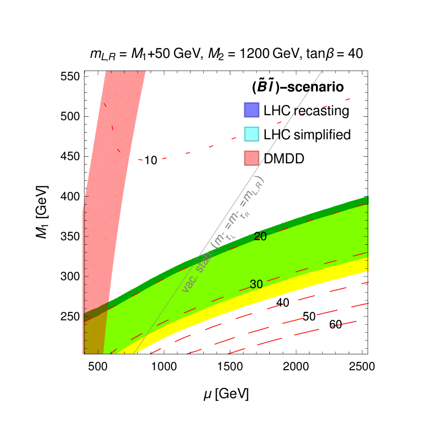
(a)

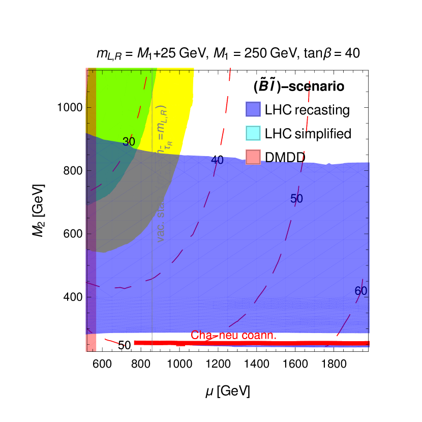
(b)

Figure 16: $(\tilde{B}\tilde{l})$-scenario with either $M_{2}=1200$ GeV fixed or $M_{1}=250$ GeV fixed. For the remaining parameter values see the plots. The red dashed contours correspond to values of $a_{\mu}$ as indicated in the legend on the right; the yellow/green coloured regions correspond to the $1\sigma$ bands corresponding to the BNL deviation (6) and the new deviation including FNAL (7), and their overlap. For the $\tan\beta$-reinterpretation see caption of Fig. 15. The (light) red shaded regions are excluded by dark matter direct detection if the LSP is assumed stable; the blue shaded region corresponds to the limits from the LHC recasting, see Fig. 20 and text for details. These plots do not contain regions excluded by the additional LHC limits implemented in a simplified way. The red thick solid line in the right plot corresponds to the parameter strip where chargino-neutralino coannihilation is possible; directly below this strip a tiny region is excluded by the LHC-constraint from compressed masses, Ref. [482], but we verified that this does not exclude the chargino-neutralino coannihilation region. The gray thin line corresponds to the vacuum stability constraint of Ref. [176]; it applies in case the left- and right-handed stau-masses are set equal to the smuon/selectron masses and excludes the points to the right, i.e. with larger $\mu$.

The $(\tilde{B}\tilde{l})$-scenario is characterized by a Bino-like LSP and sleptons significantly lighter than $700$ GeV. Given current LHC constraints it is viable if the mass splitting between sleptons and the LSP is sufficiently small, $m_{\text{L},\text{R}}-M_{1}\lesssim 100$ GeV (for masses below around 200 GeV and very small splittings additional constraints from compressed-mass searches become relevant). The dark matter relic density can be correctly achieved by either ${\tilde{l}}$/${\tilde{\tau}}$ or $\chi^{\pm}$-coannihilation by appropriate fine-tuning of parameters as discussed below. The scenario is illustrated in Fig. 16. The left plot Fig. 16(a) shows results in the $\mu$–$M_{1}$-plane. The Wino mass is fixed to the rather high value $M_{2}=1200$ GeV, safely but not too far above the chargino mass limit (64b), and the mass splitting $m_{\text{L},\text{R}}-M_{1}=50$ GeV. The right plot Fig. 16(b) shows results in the $\mu$–$M_{2}$-plane, while the Bino and slepton masses are fixed to the rather light values $M_{1}=250$ GeV and $m_{\text{L},\text{R}}=275$ GeV. In both plots the shown quantities are not very sensitive to the choice of the mass splitting, so the plots are representative for a wider range of values for $m_{\text{L},\text{R}}-M_{1}$.

The red dashed lines and yellow/green coloured regions show the contours of $a_{\mu}$ and $1\sigma$ regions corresponding to the measurements from BNL only and the average including FNAL. The behaviour of $a_{\mu}$ in this $(\tilde{B}\tilde{l})$-scenario is dominated by the WHL and BLR contributions of Eqs. (49,62) and can be well understood via these approximations. The WHL contributions dominate in the left plot at large $M_{1}$ and very small $\mu$ and in the right plot at $\mu\lesssim 1$ TeV; in these regions $a_{\mu}^{\text{SUSY}}$ decreases with increasing $\mu$. The BLR contributions are linearly enhanced by $\mu$ and dominate at large $\mu$ in both plots. As the plots show very large $a_{\mu}^{\text{SUSY}}$ can be obtained both for large $\mu$, where the BLR-contribution dominates, and for small $\mu$ with WHL-dominance.

LHC-constraints obtained by the recasting described in Sec. 6.2 are displayed by the blue shaded region in the plots. The parameter space of the left plot Fig. 16(a) is entirely allowed (more details on the recasting are exhibited in the Appendix), even where the Higgsino-like chargino is light. The right plot Fig. 16(b) shows the expected large excluded region approximately for $300\text{ GeV}<M_{2}<900\text{ GeV}$. It is excluded by the chargino/slepton channel search of Refs. [487, 520], see Eq. (64). The recasting shows again that the Wino-like charginos are significantly more constrained than Higgsino-like charginos and that the exclusion region is smaller than in the simplified-model interpretation of Eq. (64b). An additional strip of parameter space at around $M_{2}\approx M_{1}-5$ GeV (in which case the mass eigenvalues satisfy $m_{\chi^{\pm}_{1}}-m_{\chi^{0}_{1}}\approx 15$ GeV) is excluded by the recasting of the CMS compressed-mass search of Ref. [482].

Regarding dark matter it is well known that in case of a Bino-like LSP in the considered mass range the relic density is too high unless some coannihilation mechanism is active. In our case there are three options: chargino-, stau- or slepton-coannihilation (see also the review [537]). The possibility of chargino-coannihilation takes place in the parameter space where $m_{\chi^{\pm}_{1}}-m_{\chi^{0}_{1}}\approx 25$ GeV in the right plot, shown as the thick red line around $M_{2}=255$ GeV. Here the relic density takes the measured value (8) without further tuning of the slepton masses. Everywhere else in the two plots the relic density can be correctly explained via slepton- or stau-coannihilation by slightly finetuning the slepton and/or stau masses. Since there is no unique way to achieve the required coannihilation we do not carry out this finetuning but fix the parameters as described above for the evaluation of all other observables. In this way the plot is representative for all these cases.

Assuming now that the relic density is correctly explained, constraints from dark matter direct detection become relevant. The constraints from direct detection experiments are shown as the (light) red shaded bands; they exclude a large portion of the parameter space with small $\mu$, implying $\mu\gtrsim 600\ldots 800$ GeV in the plot. This reflects the well-known need for small gaugino–Higgsino mixing and a significant mass gap between the LSP and the Higgsino mass $\mu$, see also Sec. 6.2 and footnote 35.

The thin solid gray line in the plots corresponds to the vacuum stability constraint of Ref. [176] on stau-mixing already explained around Eq. (63). It excludes the large-$\mu$ region to its right under the condition that both left- and right-handed stau masses are as light as the smuon/selectron masses. This upper limit on $\mu$ thus applies in particular if stau-coannihilation and $m_{\tilde{\tau}_{\text{L}}}\approx m_{\tilde{\tau}_{\text{R}}}$ is assumed. Then the limit on $\mu$ significantly reduces the region in which the BLR-contributions to $a_{\mu}^{\text{SUSY}}$ dominate. The vacuum stability constraint can be evaded and larger $\mu$ and large $a_{\mu}^{\text{SUSY}}$ for heavier $M_{1}$ remain possible under the assumption that one stau or both staus are heavier. This can be compatible with a dark matter explanation either in the case of selectron/smuon–coannihilation, or in the case of stau–coannihilation with strongly non-universal left-/right-handed staus.

In summary, the $(\tilde{B}\tilde{l})$-scenario allows the following three parameter regions with large $a_{\mu}^{\text{SUSY}}$. The first region is in the lower left of Fig. 16(a) and the upper left of Fig. 16(b) between the dark matter and vacuum stability constraints on $\mu$. It involves $\mu$ around the 1 TeV scale and is allowed by all constraints even if we assume completely universal sleptons $m_{\text{L},\text{R}}\approx m_{\tilde{\tau}_{\text{L},\text{R}}}$. Here dark matter constraints can be explained by stau and/or slepton coannihilation and the $a_{\mu}$ result can be accommodated easily via the large BLR contributions. The new world average result for $\Delta a_{\mu}$ including FNAL can be explained well for $M_{1}\lesssim 300$ GeV and $\tan\beta=40$. As shown by Fig. 16(b), $M_{2}$ can be as low as around $900$ GeV for our choice of $M_{1}=250$ GeV, while for larger $M_{1}$ the LHC-limit on $M_{2}$ would relax slightly, and WHL-contributions could further increase $a_{\mu}^{\text{SUSY}}$. The second region is to the right of the vacuum stability lines where $\mu$ is in the multi-TeV region and $a_{\mu}^{\text{SUSY}}$ is further increased by the BLR contributions. The region is viable if at least one stau is sufficiently heavier. The dark matter relic density can then be generated via slepton or $\tilde{\tau}_{1}$ coannihilation. Here an explanation of $\Delta a_{\mu}$ is widely possible. The LSP mass can be heavier than $300$ GeV, and the large white regions in Fig. 16(b) and lower right corner of Fig. 16(a) mean that $\Delta a_{\mu}^{\text{2021}}$ can be explained for $\tan\beta<40$ according to the right axis of the legend plot. The third region is the patch of parameter space close to the lower border of Fig. 16(b). Here the Bino-like LSP, the Wino and the sleptons are all light and close in mass. This patch of parameter space allows in particular to generate dark matter via chargino-coannihilation, and it leads to very large $a_{\mu}^{\text{SUSY}}$ for any value of $\mu$ above the dark matter limit. Here again the updated deviation $\Delta a_{\mu}^{\text{2021}}$ can be explained for $\tan\beta<40$.

The recent model-building literature has put forward a variety of constructions leading to our second parameter region with light sleptons and very heavy $\mu$, where $a_{\mu}^{\text{SUSY}}$ is dominated by the BLR-contributions. These constructions are particularly motivated in view of the LHC constraints on the coloured SUSY particles and the Higgs mass. Clearly, a straightforward conclusion from such constraints is that gluino and top-squark masses are in the (multi-)TeV region. Via renormalization effects these masses can enter the electroweak symmetry breaking relations, and in many models very large $\mu$ in the multi-TeV region is then necessary in order to cancel such effects and allow a Higgs-VEV compatible with observations [230, 228, 215].

Many concrete constructions are inspired by universality ideas but involve some degree of non-universality to accommodate all existing constraints. One class of such models with multi-TeV-scale $\mu$ involves non-universal sfermion masses. General models with non-universal sfermion masses (but universal gaugino masses) have been constructed and investigated in Refs. [196, 223], where $(\tilde{B}\tilde{l})$-like scenarios with $\mu\sim 10$ TeV were identified as promising. A specific kind of sfermion non-universality was considered in Refs. [228, 173, 207], where the third generation of sfermions is assumed heavier than the first two, but universality between squarks and sleptons at some high scale is retained. Up-to-date LHC constraints on gluino and Wino masses then imply that non-universal gaugino masses are almost unavoidable unless one allows an unstable charged slepton LSP [228].

Another class of models retains universality of all scalar soft SUSY-breaking masses but allows non-universal gaugino masses. In this case again, the scenario of Fig. 16 with very large $\mu$ is the only option to obtain significant $a_{\mu}^{\text{SUSY}}$ [174, 181, 184, 224].

We mention that the scenario with $\mu$ in the multi-TeV region is also important to obtain large $a_{\mu}^{\text{SUSY}}$ in the context of various specific model constructions, such as models based on Pati-Salam symmetry [194] (here, at the same time light Winos are preferred), models with usual GUT constraints but extra vectorlike matter fields [200, 216], and in a hybrid gauge-gravity mediation model with only four free parameters [206].

6.4.3 $(\tilde{W}\tilde{l})$-scenario with light sleptons and Wino

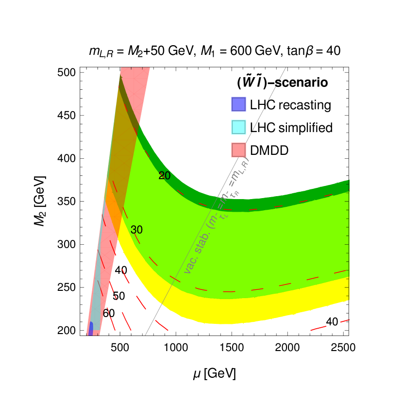
(a)

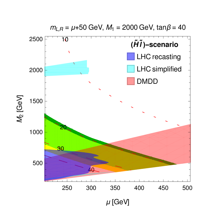
(b)

Figure 17: (a) $(\tilde{W}\tilde{l})$-scenario. (b) $(\tilde{H}\tilde{l})$-scenario. For parameter values see the plots and the text. The red dashed contours correspond to values of $a_{\mu}^{\text{SUSY}}$ as indicated in the legend on the right; the yellow/green coloured regions correspond to the $1\sigma$ bands corresponding to the BNL deviation (6) and the new deviation including FNAL (7), and their overlap. For the $\tan\beta$-reinterpretation see caption of Fig. 15. The red shaded region is excluded by dark matter direct detection if the LSP is assumed stable; the blue shaded regions correspond to the limits from the LHC recasting, see Fig. 20 for details. The cyan shaded region corresponds to the additional LHC limits implemented in a simplified way; in both plots the slepton search (67), Ref. [490] excludes a narrow strip at small $\mu$ and $M_{2}$, where the slepton–LSP mass splitting is largest. In the the right plot the compressed-mass searches of Ref. [528] exclude another small region at large $M_{2}$, which enters the LSP mass via mixing. The thin solid gray line corresponds to the vacuum stability constraint of Ref. [176]; it applies in case the left- and right-handed stau-masses are set equal to the smuon/selectron masses and excludes the points to its right, i.e. with larger $\mu$.

The $(\tilde{W}\tilde{l})$-scenario involves a Wino-like LSP and sleptons significantly lighter than 700 GeV. Current LHC-constraints on sleptons allow this scenario provided the slepton–LSP mass splitting is sufficiently small. The scenario is illustrated in Fig. 17(a) in the $\mu$–$M_{2}$-plane. The mass splitting is chosen as $m_{\text{L},\text{R}}=M_{2}+50$ GeV, but the plotted quantities are not very sensitive to this choice. By definition of the scenario, the Bino mass is assumed to be heavier than the Wino mass. Since the Bino mass is also not strongly constrained by LHC data we fix it to $M_{1}=600$ GeV, an intermediate value which is always heavier than $M_{2}$ in the plot but still allows significant BLR-contributions to $a_{\mu}^{\text{SUSY}}$.

The behaviour of $a_{\mu}^{\text{SUSY}}$ (red dashed lines and yellow/green coloured regions) in this scenario with a Wino-like LSP is similar to the previous one in the case of a Bino-like LSP. The $a_{\mu}^{\text{SUSY}}$-contours in Figs. 16(a), 16(b) and 17(a) have a similar shape. For small $\mu$ the WHL-contributions of Eqs. (49,62) dominate, and for $\mu\gtrsim 1500$ GeV the BLR-contributions to $a_{\mu}^{\text{SUSY}}$ dominate. An important difference is that the Wino-like LSP scenario allows very low Wino masses without the need for finetuning $M_{1}\approx M_{2}$ as e.g. in Fig. 16(b). Hence the WHL-dominance region is wider in the $(\tilde{W}\tilde{l})$-scenario. In all of this WHL-dominance region the actual choice of $M_{1}=600$ GeV is inconsequential. This choice is important for $\mu\gtrsim 1500$ GeV, where the BLR-contributions dominate and $a_{\mu}^{\text{SUSY}}$ rises with $\mu$. Higher choices of $M_{1}$ would reduce $a_{\mu}^{\text{SUSY}}$ in this region.

The recasting of the ATLAS chargino search [487] excludes only a tiny blue shaded region in the plot at $M_{2},\mu\lesssim 220$ GeV, where both charginos and the sleptons are similar in mass. In addition the cyan shaded narrow strip at small $\mu$ corresponds to the additional LHC limits implemented in a simplified way as discussed in Sec. 6.2. The specific analysis relevant here is the slepton search (67), Ref. [490]. It excludes this cyan parameter strip, where the splitting between the slepton and LSP mass eigenvalues is largest.

The plot shows the dark matter direct detection limit as a red shaded band. It is well-known that a Wino-like LSP cannot produce the observed relic density unless the Wino mass is in the multi-TeV region, for a recent account see Ref. [553]. In the mass region of interest for us, we obtained a Wino-LSP relic density which is typically a factor $10\ldots 100$ smaller than the observed relic density. Nevertheless, the LSP–nucleon cross sections depend on the Wino–Higgsino mixing and are rather high. Hence the dark matter direct searches imply significant lower limits on the Higgsino mass $\mu$ of around $300\ldots 800$ GeV, see also footnote 35. This limit could only be circumvented by dropping the assumption of a stable LSP, e.g. by assuming R-parity violation of LSP-decays into light gravitinos.

The thin solid gray line in the plot corresponds to the vacuum stability constraint of Ref. [176]. It applies if the left- and right-handed stau-masses are both set equal to the smuon/selectron masses. In such a case of slepton universality an upper limit on $\mu$ exists which essentially eliminates the region in which the BLR-contribution to $a_{\mu}^{\text{SUSY}}$ dominates.

In summary, the $(\tilde{W}\tilde{l})$-scenario can easily accommodate $\Delta a_{\mu}$ as large as the deviation $\Delta a_{\mu}^{\text{2021}}$ or even larger. Specifically e.g. the new world average (7) can be explained for $\tan\beta=40$ with universal slepton masses and an LSP mass around $M_{2}=350$ GeV and $\mu=800$ GeV. Higher masses, in particular higher $\mu$ are also possible. For lower masses much smaller values of $\tan\beta$ can be sufficient. There are essentially no LHC constraints on this scenario as long as the mass splitting between sleptons and the LSP are sufficiently small. Dark matter direct detection enforces lower limits on $\mu$, still leaving a wide parameter space in which the WHL-contributions to $a_{\mu}^{\text{SUSY}}$ are dominant and large. If slepton universality is assumed including staus, vacuum stability imposes an upper limit on $\mu$; larger $\mu$ is possible if (at least one) heavy stau is assumed and provides further parameter space with large $a_{\mu}^{\text{SUSY}}$.

Again we provide a brief survey of model building efforts which lead to constructions like the $(\tilde{W}\tilde{l})$-scenario with a Wino-like LSP, light sleptons and very large $\mu$. Ref. [230] has constructed an extreme variant of such a model with Wino-like LSP and slepton masses around 500 GeV based on Higgs-anomaly mediated SUSY-breaking [230, 205, 178]; that construction produces $\mu\gtrsim 25$ TeV. Ref. [221] shows that a similar scenario which involves both light Wino and Bino can follow from gaugino+Higgs-mediated SUSY breaking. Ref. [336] has also embedded a $(\tilde{W}\tilde{l})$-like scenario in a UV-model based on Higgs-mediated SUSY breaking. Such scenarios also had the potential to explain not only $\Delta a_{\mu}$ but also the smaller deviation in the electron magnetic moment $a_{e}$ [334, 336] (see however footnote 26).

6.4.4 $(\tilde{H}\tilde{l})$-scenario with light sleptons and Higgsino

The $(\tilde{H}\tilde{l})$-scenario is characterized by a Higgsino-like LSP and sleptons significantly lighter than 700 GeV. Again, in view of current LHC-constraints the slepton–LSP mass splitting cannot be much larger than 100 GeV. The scenario is illustrated in Fig. 17(b) in the $\mu$–$M_{2}$-plane. We again fix the mass splitting $m_{\text{L},\text{R}}=\mu+50$ GeV and we set the Bino mass to $M_{1}=2000$ GeV as reference values, although the considered observables are not very sensitive to this choice (except that significantly lower $M_{1}$ can lead to conflict with dark matter direct detection limits).

The behaviour of $a_{\mu}^{\text{SUSY}}$ shown by the red dashed lines and yellow/green coloured regions is quite different from the one in the previous two scenarios. Since the Higgsino mass $\mu$ is small, only the WHL-contributions of Eqs. (49,62) are important. For this reason the result shows the generic $1/M_{\text{BSM}}^{2}$-behaviour explained in Sec. 2 and drops quickly both with increasing $\mu$ or increasing $M_{2}$, while the choice of $M_{1}$ has not much influence. Still, e.g. if $\mu=300$ GeV the BNL deviation can be explained at the 1$\sigma$ level even for $M_{2}=1$ TeV.

The constraints from LHC-recasting, shown in blue, are rather strong. They originate from the chargino/slepton channel searches of Eq. (64), Refs. [487, 520]. Compared to e.g. Fig. 20 now $\mu$ instead of $M_{1}$ takes the role of the LSP-mass, and the recasting shows that the resulting limits on the Wino-like chargino mass and thus on $M_{2}$ are weaker than in Fig. 20, extending only up to $M_{2}=700$ GeV in Fig. 17(b). The plot also shows additional cyan shaded parameter regions, which are subject to additional LHC-constraints implemented in a simplified way. Here, both the slepton search of Ref. [490] and the compressed-mass searches of Ref. [528] exclude small regions at small $M_{2}$ close to the $M_{2}=\mu$ boundary and at large $M_{2}\approx 2$ TeV, close to the bino mass. In both regions, neutralino mixing happens to lead to LSP–next-to-LSP mass splittings which are excluded. Though not visible in the plot we mention that the same compressed-mass searches also impose limits on the Higgsino-like chargino/neutralino system and thereby exclude parameter space with $\mu<200$ GeV.

It is well known that a Higgsino-like LSP cannot produce the observed relic density for such light Higgsinos as considered here. Still there are relevant limits from dark matter direct detection experiments [554]. In the mass region of interest for us, we find that the Higgsino-LSP relic density is typically a factor 10 smaller than the observed relic density. This value is higher than the relic density in the previous case of a Wino-like LSP. As a result, stronger dark matter direct detection limits are obtained on $M_{2}$, shown as the red shaded band. In the plot they require $M_{2}\gtrsim 500\ldots 1500$ GeV, depending on $\mu$. As before, the dark matter direct detection limits apply only under the assumption that the Higgsino-like LSP is stable.

In summary, the $(\tilde{H}\tilde{l})$-scenario is strongly constrained by LHC chargino searches and by dark matter direct detection constraints (if the LSP is assumed to be stable). Still it allows values of $M_{2}$ as small as around $700$ GeV and $\mu$ around $200$ GeV which lead to $a_{\mu}^{\text{SUSY}}$ as large as $30\times 10^{-10}$, but outside this small corner of parameter space the values of $a_{\mu}^{\text{SUSY}}$ quickly drop. The average deviation can be explained at the $1\sigma$ level for LSP masses up to $350$ GeV for $\tan\beta=40$. At the $2\sigma$ level, much higher LSP masses are possible.

In the model building literature, Ref. [231] has considered a scenario of the $(\tilde{H}\tilde{l})$-type with significant mass gap between the Higgsino-LSP and the two gauginos, motivated within the context of a model with seesaw mechanism and SO(10) GUT constraints on the gaugino masses but non-universal scalar masses. Although electroweak LHC and DMDD constraints are not considered, this reference also finds only small viable contributions to $a_{\mu}^{\text{SUSY}}$ as a result of model-specific correlations to flavour-violating observables.

6.4.5 $(\tilde{B}\tilde{W}\tilde{H})$-scenario with light charginos

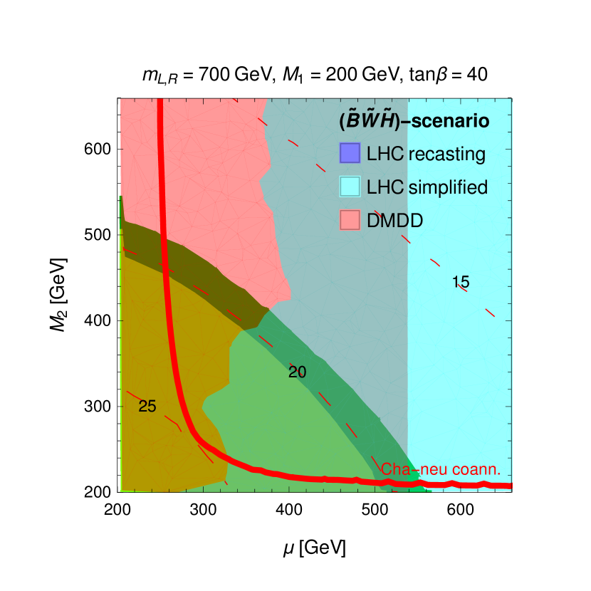
(a)

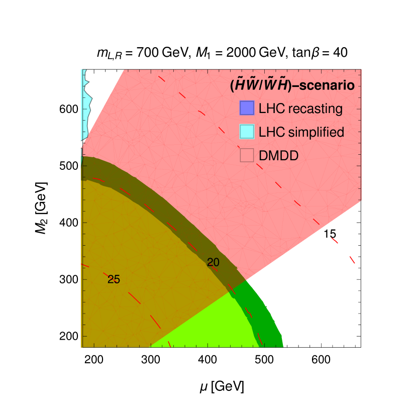
(b)

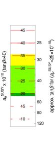
Figure 18: (a) $(\tilde{B}\tilde{W}\tilde{H})$-scenario. (b) $(\tilde{H}\tilde{W}/\tilde{W}\tilde{H})$-scenario. For parameter values see the plots and the text. The red dashed contours correspond to values of $a_{\mu}^{\text{SUSY}}$ as indicated in the legend on the right; the yellow/green coloured regions correspond to the $1\sigma$ bands corresponding to the BNL deviation (6) and the new deviation including FNAL (7), and their overlap. For the $\tan\beta$-reinterpretation see caption of Fig. 15. The red shaded region is excluded by dark matter direct detection if the LSP is assumed stable; in the left plot this red region is the rectangle extending up to $\mu\approx 540$ GeV. Both plots do not contain regions excluded by the LHC recasting. The cyan shaded regions correspond to the additional LHC limits implemented in a simplified way. In the left plot the cyan region is the large region extending from $\mu\gtrsim 300\ldots 400$ GeV to the right (it is partially overlaid with dark matter and $a_{\mu}^{\text{SUSY}}$-regions), it mainly arises from the stau-channel chargino search (66), Ref. [524]; it is valid if light staus are assumed for stau-coannihilation. The red thick line in the left plot corresponds to the parameter strip where chargino-neutralino coannihilation is possible; in this region the dark matter relic density can be correctly described without light staus and the LHC-constraint does not apply.

The remaining scenarios differ from the previous ones in that they involve two light charginos, while the sleptons are not assumed particularly light. The $(\tilde{B}\tilde{W}\tilde{H})$-scenario discussed here assumes both charginos to be lighter than the sleptons, but the Bino-like neutralino to be the LSP. Hence $M_{1}<M_{2},\mu$ with no particular order between $M_{2}$ and $\mu$. The scenario is illustrated in Fig. 18(a). In the figure we set $m_{\text{L},\text{R}}=700$ GeV, safely but not too far above the maximum LHC-limit of Ref. [490]. We also fix $M_{1}=200$ GeV and show $a_{\mu}^{\text{SUSY}}$ versus LHC and dark matter constraints as a function of $M_{2}$ and $\mu$.

The behaviour of $a_{\mu}^{\text{SUSY}}$ is dominated by the WHL-contributions of Eqs. (49,62) which are suppressed by the heavy slepton masses and further suppressed if $\mu$ and/or $M_{2}$ become heavy. The maximum contribution to $a_{\mu}^{\text{SUSY}}$ in Fig. 18(a) is around $30\times 10^{-10}$; if $\mu$ and $M_{2}$ are heavier than $500$ GeV, $a_{\mu}^{\text{SUSY}}$ reaches at most $15\times 10^{-10}$ for $\tan\beta=40$ (which is just within the $2\sigma$ region of the updated deviation $\Delta a_{\mu}^{\text{2021}}$. The chosen value of $M_{1}=200$ GeV has almost no influence on $a_{\mu}^{\text{SUSY}}$. However the parameter space of this $(\tilde{B}\tilde{W}\tilde{H})$-scenario is subject to an interesting interplay of LHC and dark matter constraints.

First, since we assume the dark matter relic density to be correctly explained, the limits from dark matter direct detection are applicable, similarly to the plots in Fig. 16. In the present case with $M_{1}=200$ GeV, the region with $\mu\lesssim 540$ GeV is excluded by this constraint. The constraint is shown by the red shaded band (partially overlaid with other coloured regions). As a result the entire region with $a_{\mu}^{\text{SUSY}}>20\times 10^{-10}$ is excluded, independently of other details.

Second, in order to achieve the correct relic density for this case of a Bino-like LSP in the given mass range, some coannihilation mechanism must act. Since sleptons are heavy, the two options are either chargino-coannihilation or stau-coannihilation. Chargino-coannihilation requires a specific chargino–LSP mass splitting. In Fig. 18(a) the thick red line denotes the one-dimensional contour along which chargino-coannihilation is possible due to appropriately small mass splittings between the lightest chargino and the LSP. Along this red contour we may assume staus to be heavy (e.g. degenerate with 1st and 2nd generation sleptons or even heavier). Anywhere outside the red line we must assume at least one or both staus to be light and close to the LSP in mass for stau-coannihilation.

Finally, we can apply LHC-constraints. The constraints depend on the coannihilation mechanism and the stau masses. Along the red contour for chargino-coannihilation we assume the staus to be heavy. Then the LHC-limit from chargino searches with $Wh$-channel [521], see Eq. (65), is relevant. It turns out, however, that these limits do not exclude the chargino-coannihilation contour due to the small mass splittings. The scenario with Bino-like LSP and light charginos but heavier sleptons and staus has also been investigated thoroughly in Ref. [535], where these scenarios were found to be not constrained and in some cases fitted excesses in the data.

Everywhere outside the red contour, we need to assume stau-coannihilation and light stau(s). In this case, the constraint from chargino searches with stau-channel [524], see Eq. (66), applies. If we apply this LHC-constraint as described in Sec. 6.2, the cyan shaded region in the plot is excluded, which is essentially the entire region with $\mu\gtrsim 350$ GeV.

As a result, the combination of dark matter and LHC-constraints exclude the entire scenario with stau-coannihilation for $M_{1}=200$ GeV. Larger values of $M_{1}$ above around $300$ GeV would relax LHC limits but lead to stronger dark matter direct detection limits (see footnote 35), thus leaving little room for large contributions to $a_{\mu}$. If in the future the deviation decreases, this parameter region with significantly higher LSP masses $M_{1}$ and stau-coanihilation may become more promising.

Ref. [201] has considered $a_{\mu}$ versus LHC in the same scenario as well, however evaluated for $M_{1}\leq 50$ GeV. This smaller value of $M_{1}$ leads to larger $a_{\mu}^{\text{SUSY}}$ and weaker dark matter constraints, but also to stronger LHC exclusion limits (assuming stau masses in between $M_{1}$ and the chargino masses) essentially excluding the entire $(\mu,M_{2})$-region of interest for $a_{\mu}$. Our larger value $M_{1}=200$ GeV reduces $a_{\mu}^{\text{SUSY}}$ but also leads to a parameter region with low chargino mass allowed by LHC; however our parameter region is challenged by DMDD constraints. This comparison highlights the complementarity between $a_{\mu}$, LHC and dark matter constraints.

In summary, the entire $(\tilde{B}\tilde{W}\tilde{H})$-scenario with light staus turns out to be strongly under pressure. A remaining possibility in this $(\tilde{B}\tilde{W}\tilde{H})$-scenario is chargino-coannihilation and heavier staus: the small part of the red thick line at $\mu>540$ GeV is viable. Here $\Delta a_{\mu}$ reaches up to $20\times 10^{-10}$ for $\tan\beta=40$, which is just sufficient to accommodate the deviation (7) at the $1\sigma$ level.

The $(\tilde{B}\tilde{W}\tilde{H})$-scenario appears in an elaborate model building construction of Ref. [213] based on the Pati-Salam model with inverse seesaw mechanism for neutrino masses. The benchmark points of that reference are very similar to the region of Fig. 18(a) with $\mu\sim 450$ GeV, $M_{2}\sim 300$ GeV; however that reference does not consider DMDD constraints, which exclude such masses in our Fig. 18(a). In that model the right-handed sneutrinos provide significant additional contributions to $a_{\mu}$, enlarging the parameter space with large $a_{\mu}^{\text{SUSY}}$. A variant of the scenario has been considered in Ref. [212]. This reference investigates dark matter generation via resonances, the so-called “$Z$/$h$-funnel” regions. It shows that LHC-constraints allow the $h$-funnel region, i.e. an LSP-mass around 60 GeV, together with large $\tan\beta\gtrsim 20$ and $\mu\gtrsim 390$ GeV, which opens up additional parameter space similar to the one of Fig. 18(a).

6.4.6 $(\tilde{H}\tilde{W}/\tilde{W}\tilde{H})$-scenarios with light charginos

In the $(\tilde{H}\tilde{W}/\tilde{W}\tilde{H})$-scenarios again both charginos are lighter than the sleptons, but now the Bino mass is also heavier, so the LSP is either Wino- or Higgsino-like. Both scenarios are illustrated in Fig. 18(b) in the $\mu$–$M_{2}$-plane. Like in the previous case we set $m_{\text{L},\text{R}}=700$ GeV, safely but not too far above the LHC limit. We also set $M_{1}=2000$ GeV. This choice is not critical — it neither influences LHC-limits nor $a_{\mu}$, but it avoids limits from dark matter direct detection (which would be similar to the limits on $M_{2}$ discussed below).

The Figure shows that the values of $a_{\mu}^{\text{SUSY}}$ are very similar to the previous $(\tilde{B}\tilde{W}\tilde{H})$-case. This is no surprise since $a_{\mu}^{\text{SUSY}}$ is dominated by the WHL-contributions and the higher value of $M_{1}$ is inconsequential. Hence the new $a_{\mu}$ deviation can be generally explained if $\tan\beta$ is around $40$ or higher.

In fact, the main difference between the present scenarios and the previous $(\tilde{B}\tilde{W}\tilde{H})$-scenario is the nature of the LSP and the resulting very different dark matter and LHC constraints.

The LHC-constraints on the previous scenario were strong in case of light staus. Since now in the $(\tilde{H}\tilde{W}/\tilde{W}\tilde{H})$-scenarios there is no need to assume light staus we assume the staus to be at least as heavy as the other sleptons. As a result there are essentially no LHC constraints on the scenarios, in line with the previous case and the findings of Ref. [535]. Only the regions with very small $\mu$ or $M_{2}\lesssim 200$ GeV are subject to constraints from compressed-spectrum searches for the Higgsino- or Wino-like chargino/neutralino system. In the plot only a tiny cyan region at $\mu\approx 200$ GeV is excluded in this way, but the largest part of parameter space is allowed by LHC.

The dark matter direct detection limits apply under the assumption that the LSP is stable. As also mentioned in the context of Fig. 17 in Secs. 6.4.3 and 6.4.4, the LSP relic density is smaller than the observed value in the displayed parameter region, hence only a fraction of the observed dark matter can be explained. Nevertheless, the LSP–nucleon cross sections are sufficiently high to imply significant lower limits on the chargino masses. The limits are stronger in case of a Higgsino-like LSP and exclude the largest part of parameter space in the upper left part of the plot. The fact that current direct detection constraints exclude a large fraction of the parameter space with Higgsino-like dark matter has already been observed in Ref. [554], where also scenarios with non-thermal dark matter production and additional dark matter candidates such as axions were considered. In the case of a Wino-like LSP the dark matter relic density is smaller and the constraints from direct detection are weaker, leaving open a larger triangular region in the lower right part of the plot.

In summary, therefore, almost the entire Higgsino-like LSP region of the $(\tilde{H}\tilde{W}/\tilde{W}\tilde{H})$-scenario is excluded by the combination of LHC compressed-mass searches and dark matter direct detection. Only a small region in the upper left part of the plot around $\mu\sim 250$ GeV and $M_{2}\sim 600$ GeV remains viable. In this region, $a_{\mu}^{\text{SUSY}}$ is always smaller than $20\times 10^{-10}$ for $\tan\beta=40$ and outside the $1\sigma$ region of the new deviation $\Delta a_{\mu}^{\text{2021}}$. The Wino-like LSP region of the $(\tilde{H}\tilde{W}/\tilde{W}\tilde{H})$-scenario in the triangular bottom right region of the plot allows a larger viable parameter space, in which a $1\sigma$ explanation of $\Delta a_{\mu}^{\text{2021}}$ is possible for $\tan\beta=40$ and even a full explanation $a_{\mu}^{\text{SUSY}}=25\times 10^{-10}$ can be reached. However for smaller $\tan\beta$, the current deviation is harder to explain. In case the dark matter constraints are not applied (by assuming unstable LSP) both scenarios can accommodate $\Delta a_{\mu}$ higher than $30\times 10^{-10}$.

In the literature, several model-building efforts have led to specific constructions with mass patterns of the $(\tilde{H}\tilde{W}/\tilde{W}\tilde{H})$ kind. The scenario with either Higgsino- or Wino-like LSP can be motivated in gauge-mediated SUSY breaking [219], extended by non-minimal contributions to the soft-breaking parameters which allow the Higgs, squark and slepton scalar mass parameters to be non-universal. In addition, in the context of gauge-mediated SUSY breaking the lightest neutralino can decay into gravitinos; hence the DMDD constraints of Fig. 18(b) do not apply and the scenario of Ref. [219] provides a viable SUSY model explaining $\Delta a_{\mu}$. The Higgsino-like LSP scenario can be motivated within anomaly-mediated SUSY breaking [188], gaugino-mediated SUSY breaking [191] or in the context of electroweak finetuning considerations [195, 185]. The scenario has also been constructed in Ref. [187] as a focus-point scenario (called FPNUS or FPHGM) based on gravity mediation with non-universal scalar masses or on Higgs-gaugino mediation. All these references do not apply DMDD constraints, which may be justified by assuming R-parity violation [187]. Similar scenarios were considered in a model with pseudo-Dirac gluino [211]; there, also DMDD constraints were investigated based only on the weaker limits from LUX and PandaX, however also leading to significant constraints on parameter space. Ref. [207] also considers the $(\tilde{H}\tilde{W})$-scenario with Higgsino-like LSP, but here universality between squarks and sleptons and quark flavour constraints imply only small contributions to $a_{\mu}$.

6.5 Summary

Here we briefly summarize our main results on SUSY explanations of $\Delta a_{\mu}^{\text{2021}}$. Like for other BSM scenarios, negative results from LHC and dark matter searches have significantly reduced the viable SUSY parameter space. Simple traditionally considered cases such as the Constrained MSSM are already excluded as explanations of $\Delta a_{\mu}^{\text{BNL}}$ and now also of $\Delta a_{\mu}^{\text{2021}}$ [555, 556, 557, 558].

In our detailed phenomenological analysis we focused on the general MSSM without restrictions from GUT scale assumptions or specific SUSY breaking mechanisms. The only restrictions imposed by our analysis are a stable neutralino-like LSP which constitutes (part or all of) dark matter and the absence of flavour-violating soft SUSY-breaking parameters. For simplicity we also consider equal masses of left- and right-handed selectrons and smuons (called sleptons for short), while the stau-masses are left arbitrary. In a series of footnotes 28, 32, 36, 39 we commented on alternative cases with ultra-high $\tan\beta$ or $\mu$, enhancements via lepton-flavour violation, and the MRSSM without $\tan\beta$ enhancement. The results of our analysis are as follows.

• Scenario with heavy charginos and smuons: the MSSM scenario with generally heavy masses, corresponding to the upper right quadrant of Fig. 15 where LHC limits are trivially avoided is disfavoured as an explanation of $\Delta a_{\mu}^{\text{2021}}$. For such SUSY heavy masses, the current $a_{\mu}$ deviation can at most be explained if $\tan\beta\gg 40$ and/or $\mu\gg 4$ TeV.

• $(\tilde{B}\tilde{l})$-scenario: a promising MSSM scenario is the $(\tilde{B}\tilde{l})$-scenario with Bino-like LSP and close-by sleptons to evade LHC limits. We identified three allowed parameter regions particularly promising in view of $\Delta a_{\mu}^{\text{2021}}$: (1) Wino mass above LHC limits of around $900$ GeV (for LSP mass of $250$ GeV) and Higgsino mass $\mu$ of order $1$ TeV. Here all slepton and stau masses may be universal. (2) Wino mass as before but $\mu$ in the multi-TeV region. Here at least one stau must be heavier to avoid vacuum stability constraints. (3) Light Wino with mass similar to the Bino and slepton masses. In all regions dark matter data implies a lower mass limit on $\mu$. The relic density can be generated via stau/slepton coannihilation; in region (3) also Wino coannihilation is possible. In all these cases the result for $\Delta a_{\mu}^{\text{2021}}$ after the FNAL measurement can be easily explained in a wide range of masses and $\tan\beta$ values.

• $(\tilde{W}\tilde{l})$- and $(\tilde{H}\tilde{l})$-scenarios: the $(\tilde{W}\tilde{l})$- and $(\tilde{H}\tilde{l})$-scenarios are characterized by Wino- or Higgsino-like LSP; the sleptons are sufficiently close to the LSP to evade LHC limits. Specifically the $(\tilde{W}\tilde{l})$-scenario can lead to the largest $a_{\mu}^{\text{SUSY}}$ of any MSSM scenario in a wide parameter space via the WHL and BLR contributions: the DMDD constraints are weak and there are essentially no additional LHC constraints. The new updated $a_{\mu}$ deviation can be accommodated in a wide range of masses and $\tan\beta$ values, see Fig. 17(a). At the $1\sigma$ level and for $\tan\beta=40$ LSP masses above $400$ GeV are possible.

  In the $(\tilde{H}\tilde{l})$-scenario $a_{\mu}^{\text{SUSY}}$ is dominated only by WHL contributions, and DMDD and LHC constrain the Wino mass to be rather heavy. Hence there is an upper limit to the possible values of $a_{\mu}^{\text{SUSY}}$, but a $1\sigma$ explanation of the current $a_{\mu}$ deviation is possible for $\tan\beta=40$ and for LSP masses below $350$ GeV. However, in both cases of Wino- or Higgsino-like LSP, the dark matter relic density cannot be fully accommodated simultaneously with $\Delta a_{\mu}^{\text{2021}}$, necessitating additional non-MSSM components of dark matter such as gravitinos.

• $(\tilde{B}\tilde{W}\tilde{H})$- and $(\tilde{H}\tilde{W}/\tilde{W}\tilde{H})$-scenarios: in the $(\tilde{B}\tilde{W}\tilde{H})$- and $(\tilde{H}\tilde{W}/\tilde{W}\tilde{H})$-scenarios both charginos are assumed to be lighter than the sleptons, which in turn are constrained by LHC data. $a_{\mu}$ is rather limited in both scenarios. In the $(\tilde{B}\tilde{W}\tilde{H})$-scenario the Bino-like neutralino is the LSP and even lighter than both charginos. Outside the Bino-Wino coannihilation region this scenario is very strongly constrained by the combination of dark matter and LHC constraints. In the Bino-Wino coannihilation region, all constraints can be fulfilled for sufficiently large $\mu$, however in this region and for $\tan\beta=40$ $a_{\mu}^{\text{SUSY}}$ is almost always at least $1\sigma$ lower than the observed deviation. In the $(\tilde{H}\tilde{W}/\tilde{W}\tilde{H})$-scenarios either the Wino- or Higgsino-like neutralino is the LSP. Assuming staus as heavy as the other sleptons, there are no relevant LHC constraints. Although the full dark matter relic density is below the observed one (similarly to the $(\tilde{W}\tilde{l})$- and $(\tilde{H}\tilde{l})$-cases), direct detection constraints exist and require a mass splitting between the Higgsinos and Winos. The resulting $a_{\mu}^{\text{SUSY}}$ can be larger in case of a Wino-like LSP. Such a scenario is well able to explain the observed deviation for $\tan\beta=40$ or slightly smaller $\tan\beta$ values.

The discussion and the plots show that the general MSSM can explain the current $\Delta a_{\mu}^{\text{2021}}$ in large parameter regions which will remain hard to test at the LHC alone. More sensitive LHC measurements will however sharpen the limits on SUSY particle masses; depending on the scenario, the mass of the LSP, of the dark matter coannihilation partner, or of the Wino-like chargino mass will be further scrutinized. If the LHC search results remain negative, this, together with theoretical constraints such as the stau vacuum stability constraints, will particularly help to eliminate motivated high-scale scenarios beyond the Constrained MSSM.

Future dark matter direct detection experiments are very promising in view of MSSM explanations of $\Delta a_{\mu}^{\text{2021}}$. Both the LUX-ZEPLIN (LZ) experiment [559] and the XENONnT experiment [560] have the potential to increase the sensitivity to DMDD cross sections by more than an order of magnitude, reaching close to the irreducible neutrino background. These experiments have the potential to discover evidence for SUSY dark matter if the MSSM explanation of $\Delta a_{\mu}^{\text{2021}}$ is correct, or to significantly reduce the available parameter space. For the longer-term future, $e^{+}e^{-}$ colliders offer great potential of testing MSSM explanations of $\Delta a_{\mu}^{\text{2021}}$ more conclusively, and we refer to Refs. [548, 203] for more details. These references have shown that some part of the dark matter coannihilation parameter space can be tested at an $e^{+}e^{-}$ linear collider with $500$ GeV center-of-mass energy, while a very large part of the parameter space can be tested at a multi-TeV $e^{+}e^{-}$ collider such as CLIC [561].

7 Conclusions

15 years after the BNL $a_{\mu}$ measurement showed a tantalizing deviation from the SM theory value and following tremendous theoretical work on improving and stabilizing the SM prediction, the Fermilab E989 experiment has published its first measurement of $a_{\mu}$. The result is a strong confirmation of the BNL result and the existence of a deviation to the SM. After including the FNAL result, the new world average results in $\Delta a_{\mu}^{\text{2021}}=25.1\times 10^{-10}$, a $4.2\sigma$ deviation. It strengthens the indications for the existence of BSM physics in the lepton sector, possibly related to the muon mass generation mechanism.

Which BSM scenarios can accommodate the new Fermilab $a_{\mu}$ measurement, and what are the required parameter values? The present paper provides a detailed survey of possible explanations to answer this question. We focused on renormalizable models which were already promising in view of the previous BNL result. We asked particularly in what parameter space the models can accommodate the $a_{\mu}$ results, taking into account up-to-date constraints from LHC and dark matter searches, as well as other relevant constraints. Our survey covered simple extensions of the SM by one, two, or three new fields (required to be full SM gauge multiplets), including e.g. leptoquark and Two-Higgs doublet models, as well as a general version of the MSSM. Secs. 3, 4 also contain detailed overviews of the status of models, and summaries of our phenomenological results can be found at the end of each section.

A useful background information is that the observed deviation $\Delta a_{\mu}^{\text{2021}}$ is larger than the electroweak contributions $a_{\mu}^{\text{EW}}=15.36(0.10)\times 10^{-10}$. BSM contributions to $a_{\mu}$ are typically suppressed as $1/M_{\text{BSM}}^{2}$. Hence BSM models explaining the deviation must have nontrivial properties, and many models are excluded as explanations. The common nontrivial feature of most viable explanations is enhancements in the muon left–right chirality flip via new couplings and interactions. As explained around Eq. (11) the chirality flip enhancement is strongly related to the muon mass generation mechanism and causes related loop contributions to the muon mass. As a side note, one obtains a quite model-independent order-of-magnitude relationship: models in which the muon mass correction does not exceed $100\%$ can explain $\Delta a_{\mu}^{\text{2021}}$ only for $M_{\text{BSM}}^{\text{FNAL}}\lesssim{\color[rgb]{0,0,0}2.1\text{\ TeV}}$ according to Eq. (14). But even in such models with chirality flip enhancements an explanation of $\Delta a_{\mu}^{\text{2021}}$ requires specific, often “non-traditional” regions of parameter space.

Examples of excluded models include the red highlighted models in Tables 1, 2, many versions of leptoquark models or the familiar type I, II versions of the 2HDM. In the context of supersymmetry, familiar scenarios such as the Constrained MSSM cannot explain the deviation. Certain leptoquark and vector-like lepton models are examples which generate very large chiral enhancements, but they need non-flavour universal couplings, e.g. direct leptoquark couplings of muon to top-quark in the left- and right-handed sector.

An important outcome of the present study is that once the $a_{\mu}$ result is combined with current data from LHC and dark matter experiments, we obtain strong constraints on the detailed ways how BSM models can be realized. The only viable models of the kind discussed in Sec. 4 that do not have chirality enhancements, are particularly strongly constrained. In these models, LHC data and $\Delta a_{\mu}^{\text{2021}}$ can be accommodated simultaneously in a small slice of parameter space, however it is impossible to also account for the full dark matter relic density, see Figs. 5–8. In contrast the simple 3-field models 2F1S and 2S1F of Sec. 5 are least constrained and can accommodate $a_{\mu}$ and dark matter in a wide parameter region. The required values of the new coupling constants, however, are large and it remains to be seen how such scenarios can arise in more complete theories.

The 2HDM can accommodate the observed $\Delta a_{\mu}^{\text{2021}}$ while preserving minimal flavour violation, but only in the lepton-specific type X version or the generalized flavour-aligned 2HDM. Even in these scenarios only a tiny parameter space remains, where the new Yukawa couplings are close to their upper experimental limits and the new Higgs masses in a very narrow range below $100$ GeV, see Fig. 1. Leptoquark masses are strongly constrained by LHC to be significantly above $1$ TeV, pushing the explanation of $\Delta a_{\mu}^{\text{2021}}$ close to the region violating the fine tuning criterion on the muon mass, see Figs. 2–4.

For SUSY scenarios, the general tension between LHC mass limits and explanations of $\Delta a_{\mu}^{\text{2021}}$ is illustrated in Fig. 15. Still, the MSSM with Bino-like LSP and either stau/slepton-coannihilation or chargino coannihilation can fully explain $\Delta a_{\mu}^{\text{2021}}$ and the dark matter relic density, see Fig. 16. Apart from the constraints implied by the coannihilation mechanisms, the parameter space is wide open in the $M_{1}$–$\mu$ plane. LHC and dark matter constraints however imply mass patterns, e.g. lower limits on the Higgsino mass and two windows for the Wino mass. The case where both charginos are lighter than sleptons is very strongly constrained and may be excluded by future data from $a_{\mu}$, LHC and dark matter experiments (Fig. 18(a)). Further, in the largest part of viable parameter space the simple GUT constraint on gaugino masses $M_{1}/M_{2}\approx 1/2$ is strongly violated. The scenarios with a Higgsino-like LSP are strongly constrained and can accommodate the current $a_{\mu}$ only in a limited range of masses. Scenarios with Wino-like LSP emerge as particularly interesting (Figs. 17, 18(b)). They can accommodate $a_{\mu}$ in a vast parameter space without significant constraints; however in these scenarios the dark matter relic density can only be partially explained without additional contributions to the relic density.

These results and discussions highlight the importance of $a_{\mu}$ not only as a potential proof of BSM physics but also of a crucial constraint on models. Particularly in combination with current LHC and dark matter data, it points to specific parameter regions of models and gives crucial clues on how BSM physics can (or cannot) be realized. Since many models involve muon chirality flip enhancements and/or flavour non-universality, further experiments testing lepton flavour violation, electric dipole moments, or lepton universality are promising to uncover further properties of BSM physics. Since the muon chirality flip enhancements are related to the mass generation mechanism for the muon, also the measurement of the Higgs–muon coupling at LHC or future lepton colliders can provide a test of various explanations of $\Delta a_{\mu}^{\text{2021}}$. Further ultimate tests may be performed at a multi-TeV muon collider [562, 563, 564, 565, 566, 567].

The new Fermilab $a_{\mu}$ measurement provides the best possible starting point for future $a_{\mu}$ determinations. Exciting further progress can be expected from the Run-2–4 results of the FNAL $g-2$ experiment, the planned JPARC $g-2$ experiment [568, 569], and from further progress on SM theory including the MUonE initiative to provide alternative experimental input to the determination of the hadronic contributions to $a_{\mu}$ [570, 571].

Appendix A General $a_{\mu}$ Contributions

Here we collect generic one-loop results for BSM contributions to $a_{\mu}$. We consider a generic new fermion $F$, a new scalar $S$ and a new vector field $V$ with masses $m_{F,S,V}$. The muon can have the following general couplings to SM and these BSM particles:

$${\cal L}_{\text{muon}}=\lambda_{L}\overline{F_{R}}.S.L+\lambda_{R}\overline{F_{L}}.S.\mu+g_{L}\overline{F_{L}}\gamma^{\nu}V_{\nu}L+g_{R}\overline{F_{R}}\gamma^{\nu}V_{\nu}\mu+h.c.,$$ (75)

where $L=(v_{\mu_{L}},\mu_{L})^{T}$ corresponds to the $SU(2)_{L}$ left-handed lepton doublet, and $\mu=\mu^{\dagger}_{R}$ corresponds to the conjugate of the right-handed muon. From this Lagrangian, we can generate $6$ generic one-loop contributions, as shown in Fig. 19, where charge flows from left-to-right and the fermions and scalars in the loop are assumed to have a negative charge. Using these couplings one can calculate (through Package-X in Ref. [572])the general one-loop contributions in the $\xi=1$ (t’Hooft Feynman) gauge of the general R-$\xi$ class of gauges (see Ref. [573]) read in the heavy BSM limit $M_{BSM}\gg m_{\mu}$:

$$a^{\text{FFS}}_{\mu} =\frac{Q_{F}m_{\mu}^{2}}{16\pi^{2}m_{S}^{2}}\bigg{(}-\frac{2\lambda_{L}\lambda_{R}}{3}\frac{m_{F}}{m_{\mu}}\,F\!\begin{pmatrix}\frac{m_{F}^{2}}{m_{S}^{2}}\end{pmatrix}-\frac{(\lambda_{L}^{2}+\lambda_{R}^{2})}{12}\,E\!\begin{pmatrix}\frac{m_{F}^{2}}{m_{S}^{2}}\end{pmatrix}\bigg{)},$$ (76)

$$a^{\text{SSF}}_{\mu} =\frac{Q_{S}m_{\mu}^{2}}{16\pi^{2}m_{S}^{2}}\bigg{(}\frac{\lambda_{L}\lambda_{R}}{3}\frac{m_{F}}{m_{\mu}}\,C\!\begin{pmatrix}\frac{m_{F}^{2}}{m_{S}^{2}}\end{pmatrix}+\frac{(\lambda_{L}^{2}+\lambda_{R}^{2})}{12}\,B\!\begin{pmatrix}\frac{m_{F}^{2}}{m_{S}^{2}}\end{pmatrix}\bigg{)},$$ (77)

$$a^{\text{FFV}}_{\mu} =\frac{Q_{F}m_{\mu}^{2}}{16\pi^{2}m_{V}^{2}}\bigg{(}\frac{4(g_{L}g_{R})}{3}\frac{m_{F}}{m_{\mu}}\,C\!\begin{pmatrix}\frac{m_{F}^{2}}{m_{V}^{2}}\end{pmatrix}-\frac{(g_{L}^{2}+g_{R}^{2})}{3}\,M\!\begin{pmatrix}\frac{m_{F}^{2}}{m_{V}^{2}}\end{pmatrix}\bigg{)},$$ (78)

$$a^{\text{VVF}}_{\mu} =\frac{Q_{V}m_{\mu}^{2}}{16\pi^{2}m_{V}^{2}}\bigg{(}-3(g_{L}g_{R})\frac{m_{F}}{m_{\mu}}\,K\!\begin{pmatrix}\frac{m_{F}^{2}}{m_{V}^{2}}\end{pmatrix}-\frac{(g_{L}^{2}+g_{R}^{2})}{6}\,J\!\begin{pmatrix}\frac{m_{F}^{2}}{m_{V}^{2}}\end{pmatrix}\bigg{)},$$ (79)

$$a^{\text{VSF}}_{\mu} =\frac{Q_{V}m_{\mu}^{2}}{16\pi^{2}m_{V}}\bigg{(}\frac{(\lambda_{R}g_{L}+\lambda_{L}g_{R})}{2m_{\mu}}\,N\!\begin{pmatrix}\frac{m_{F}^{2}}{m_{V}^{2}},\frac{m_{F}^{2}}{m_{S}^{2}}\end{pmatrix}\bigg{)},$$ (80)

$$a^{\text{SVF}}_{\mu} =\frac{Q_{V}m_{\mu}^{2}}{16\pi^{2}m_{V}}\bigg{(}\frac{(\lambda_{L}g_{L}+\lambda_{R}g_{R})}{2m_{\mu}}\,N\!\begin{pmatrix}\frac{m_{F}^{2}}{m_{V}^{2}},\frac{m_{F}^{2}}{m_{S}^{2}}\end{pmatrix}\bigg{)}.$$ (81)

The one-loop functions are defined as:

$$B(x) =\frac{2(1-6x+3x^{2}+2x^{3}-6x^{2}\log{x})}{(1-x)^{4}},$$ (82)

$$C(x) =\frac{3(1-x^{2}+2x\log{x})}{(1-x)^{3}},$$ (83)

$$E(x) =\frac{2(2+3x-6x^{2}+x^{3}+6x\log{x})}{(1-x)^{4}},$$ (84)

$$F(x) =\frac{3(-3+4x-x^{2}-2\log{x})}{2(1-x)^{3}},$$ (85)

$$J(x) =\frac{7-33x+57x^{2}-31x^{3}+6x^{2}(3x-1)\log{x}}{(1-x)^{4}},$$ (86)

$$K(x) =\frac{(1-4x+3x^{2}-2x^{2}\log{x})}{(1-x)^{3}},$$ (87)

$$M(x) =\frac{(4-9x+5x^{3}+6(1-2x)x\log{x})}{(1-x)^{4}},$$ (88)

$$N(x,y) =\frac{y}{(y-1)}\frac{x(x-y)^{2}\log{x}+(x-1)((x-y)*(y-1)-(x-1)x\log{(x/y)})}{(1-x)^{2}(x-y)^{2}}.$$ (89)

Here $x=m_{F}^{2}/m_{S}^{2}$ for FFS and SSF diagrams, $x=m_{F}^{2}/m_{V}^{2}$ for FFV, VVF, VSF, and SVF diagrams, and $y=m_{F}^{2}/m_{S}^{2}$ for VSF and SVF diagrams. The above one-loop functions with one argument have the limits $\lim_{x\rightarrow 1}$OneLoop$(x)=1$ (Except for $J(x)$, $K(x)$, and $M(x)$ which have the limits $7/5$, $2/3$, and $3/2$) and $\lim_{x\rightarrow\infty}$OneLoop$(x)=0$, and have the following limits as $x\rightarrow 0$:

$$\underset{x\rightarrow 0}{\text{lim }}B(x)\rightarrow 2, \underset{x\rightarrow 0}{\text{lim }}C(x)\rightarrow 3, \underset{x\rightarrow 0}{\text{lim }}E(x)\rightarrow 4, \underset{x\rightarrow 0}{\text{lim }}F(x)\rightarrow\infty,$$

$$\underset{x\rightarrow 0}{\text{lim }}J(x)\rightarrow 7, \underset{x\rightarrow 0}{\text{lim }}K(x)\rightarrow 1, \underset{x\rightarrow 0}{\text{lim }}M(x)\rightarrow 4.$$

The formulas needed e.g. for SUSY diagrams in mass-insertion approximation are given by

$$F_{a}(x,y) =-\frac{F(x)-F(y)}{3(x-y)},$$ (90a)

$$F_{b}(x,y) =-\frac{C(x)-C(y)}{6(x-y)},$$ (90b)

$$\tilde{F}_{a}(x,y) =-\frac{xF(x)-yF(y)}{3\left(\frac{1}{x}-\frac{1}{y}\right)}.$$ (90c)

They have the limits $$F_{a}(1,1)=1/4 F_{b}(1,1)=\tilde{F}_{a}(1,1)=1/12$$ and .

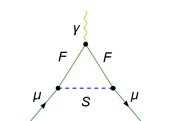
(a)

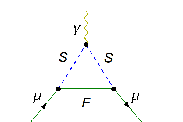
(b)

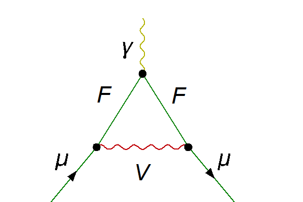
(c)

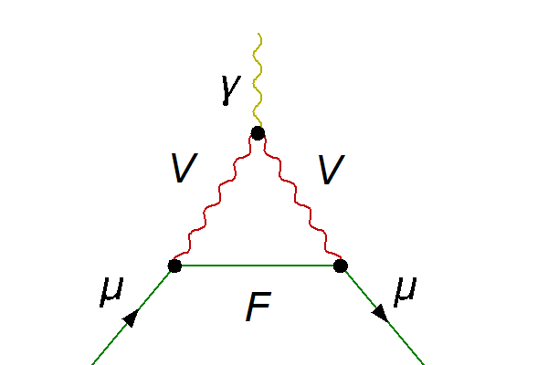
(d)

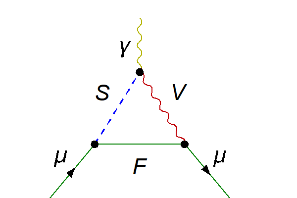
(e)

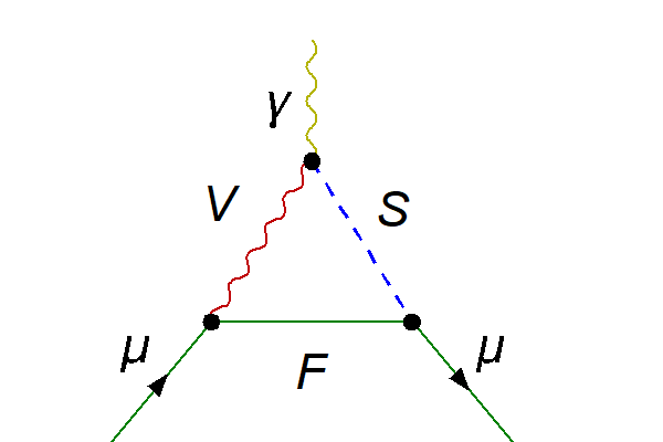
(f)

Figure 19: Diagrams producing general contributions to $a_{\mu}$. Reading left-to-right, top-to-bottom, the FFS diagram 19(a), the SSF diagram 19(b), the FFV diagram 19(c), the VVF diagram 19(d), the VSF diagram 19(e), and the SVF diagram 19(f).

Appendix B Details on LHC-constraints on SUSY parameter regions

In section 6.2 we described our procedure for recasting LHC-constraints on the SUSY parameter space; the procedure was then applied in section 6.4 to investigate the impact of LHC-constraints on the SUSY parameter space. Here we provide further details on the recasting.

In Fig. 20 we illustrate the recasting by reproducing the exclusion contour of the ATLAS chargino/neutralino search of Ref. [487], Fig. 8c. Like in that reference, we have generated MSSM parameter points with mass hierarchy $M_{1}<m_{\text{L},\text{R}}<M_{2}<\mu$, i.e. Bino-like LSP, intermediate sleptons of the 1st and 2nd generation, and a Wino-like pair of $\chi_{2}^{0}/\chi_{1}^{\pm}$. We allowed the slepton mass ratio parameter $x=(m_{\text{L},\text{R}}-m_{\chi_{1}^{0}})/(m_{\chi_{1}^{\pm}}-m_{\chi_{1}^{0}})$ to be in the range $1/3<x<2/3$, while Ref. [487] fixed $x=1/2$. The thick solid blue contour in our Fig. 20 corresponds to points where the predicted signal yield for at least one signal region is equal to the respective ATLAS 95% C.L. upper limit. It can be seen that this contour tracks the corresponding 95% C.L. contour of Ref. [487], Fig. 8c, very well, i.e. to within 50 GeV. To illustrate the gradient we also show the thick dashed blue contour, corresponding to points where the predicted signal yield is three times higher than the respective ATLAS upper limit. Finally we also show blue coloured regions corresponding to different values of the largest effective $(-2\ln{\cal L}_{\text{eff}})$ of any implemented analysis (in this figure, this is always the 3-lepton channel analysis of Ref. [487]). We find that numerically the contour with $(-2\ln{\cal L}_{\text{eff}})^{\text{Max}}=6$ tracks very well the 95% C.L. contour. We checked that the same would be true for most plots of our section 6.4 (the exceptions are very few cases where such a comparison is not possible because the relevant contribution to $(-2\ln{\cal L}_{\text{eff}})^{\text{Max}}$ comes from the CMS analysis of Ref. [482] for compressed spectra, which does not provide individual 95% C.L. upper signal limits).

Fig. 20 shows that the recasting reproduces the corresponding original ATLAS exclusion contour very well. On the other hand, several of the scenarios presented in Sec. 6.4, particularly Figs. 16(a), and 18 turned out to be entirely unconstrained by the LHC recasting. Hence we present here quantitative results of our recasting analysis, to confirm these statements and to expose further details.

We confirmed that out of all ATLAS and CMS analyses implemented in GAMBIT/ColliderBit, the ATLAS electroweakino search of Ref. [487] is most sensitive in the parameter regions in Figs. 16 and 18. Within this ATLAS search, the 3-lepton channel is most sensitive. The 3-lepton channel in turn is divided into 11 signal regions. Hence we will mainly focus on the results for these 11 signal regions in the following.

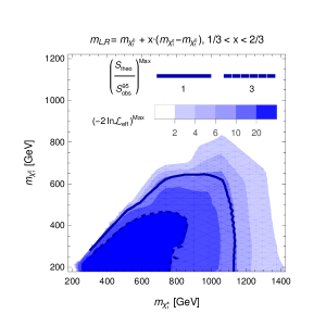
Figure 20: Recasting of the exclusion limits corresponding to Ref. [487], Fig. 8c. The generated MSSM parameter points have the mass hierarchy $M_{1}<m_{\text{L},\text{R}}<M_{2}<\mu$, i.e. Bino-like LSP, intermediate sleptons of the 1st and 2nd generation, and a Wino-like pair of $\chi_{2}^{0}/\chi_{1}^{\pm}$. The slepton masses satisfy $x=(m_{\text{L},\text{R}}-m_{\chi_{1}^{0}})/(m_{\chi_{1}^{\pm}}-m_{\chi_{1}^{0}})$ with $1/3<x<2/3$. The thick solid blue contour can be directly compared to the 95% C.L. exclusion contour of Ref. [487], Fig. 8c; the thick dashed blue contour corresponds to points where the predicted signal yield is three times higher than the respective ATLAS upper limit in at least one signal region. The blue coloured regions correspond to various values of the maximum effective $(-2\ln{\cal L}_{\text{eff}})$ of any analysis implemented in GAMBIT/ColliderBit. The plots in section 6.4 show only the region corresponding to $(-2\ln{\cal L}_{\text{eff}})=6$, which is very close to the line where $\left(S_{\text{theo}}/S_{\text{obs}}^{95\%}\right)\geq 1$ for at least one signal region; see text for more details.

Tables 4 and 5 define example SUSY parameter points and present detailed results. The first four parameter points represent the $(\tilde{B}\tilde{l})$-, $(\tilde{B}\tilde{W}\tilde{H})$-, and $(\tilde{H}\tilde{W})$-scenarios. They are examples obtained in a parameter scan with particularly bad fit to experiment, i.e. particularly small likelihood ratio (but they are still not excluded). The other two points represent the excluded region in Fig. 20 with high or low chargino mass.

The columns $\ln{\cal L}_{\text{eff}}^{\text{analysis}}$ of Tab. 4 display effective analysis-specific log-likelihood differences $\ln{\cal L}_{\text{eff}}^{\text{analysis}}\equiv\ln{\cal L}_{\text{SR${}^{\text{max}}$}}^{\text{analysis}}$, where $\text{SR}^{\text{max}}$ denotes the signal region of the respective analysis with the highest expected sensitivity, see Sec. 6.2 and Ref. [530]. The analyses are the ATLAS analyses of Ref. [487] for the 3-lepton, 2-lepton 0-jet and 2-lepton+jets channels, and to the CMS analyses of Ref. [520] for the 2-same sign lepton and 3-lepton channels. The table shows that the ATLAS and CMS 3-lepton channels are most sensitive for all parameter points.

Tab. 5 shows the results obtained by ColliderBit for the 11 invidual signal regions of the ATLAS 3-lepton analysis and compares to the ATLAS results. The most important observation is that all signal yield predictions of the first four parameter points are far smaller than the ATLAS signal $95\%$ C.L. upper limits. The entries which come relatively closest, i.e. which lead to the smallest negative log-likelihood difference, are highlighted in boldface. A second observation is that these entries are not always identical to the ones selected by ColliderBit for evaluating the effective log-likelihood difference for the next-to-last column of Tab. 4. The reason [530] is that the selection is done assuming that the observed counts match the background expectation; however for the WZ-1Jc and slep-a signal regions this assumption is not true ($N_{\text{obs}}:N_{\text{exp}}=4:1.3\pm 0.3$ and $N_{\text{obs}}:N_{\text{exp}}=4:2.2\pm 0.8$ respectively).

On the other hand, for the two parameter points of the excluded region in Fig. 20 we observe that the high-mass point is indeed excluded by the slep-e signal region, and the low-mass point is excluded by a variety of signal regions by a large margin.

$\begin{array}[]{|c|c|c|c|c|c|c|c|c|c|c|c|}\hline\cr\text{Point}&M_{1}&M_{2}&\mu&m_{L,R}&\ln{\cal L}_{\text{eff}}^{\text{ATLAS\_3Lep}}&\ln{\cal L}_{\text{eff}}^{\text{ATLAS\_2Lep0Jets}}&\ln{\cal L}_{\text{eff}}^{\text{ATLAS\_2LepPlusJets}}&\ln{\cal L}_{\text{eff}}^{\text{CMS\_2SSLep}}&\ln{\cal L}_{\text{eff}}^{\text{CMS\_3Lep}}\\ \hline\cr\text{$(\tilde{B}\tilde{l})_{1}$}&200&1200&630&250&-0.45&0.33&0.003&0.002&0.25\\ \hline\cr\text{$(\tilde{B}\tilde{W}\tilde{H})_{1}$}&200&296&346&700&0.50&0.07&0.04&0.05&-0.24\\ \hline\cr\text{$(\tilde{B}\tilde{W}\tilde{H})_{2}$}&200&329&388&700&1.05&0.16&-0.37&0.05&-0.35\\ \hline\cr\text{$(\tilde{H}\tilde{W})_{1}$}&2000&239&162&700&-0.83&0.17&-0.04&-0.04&-0.1\\ \hline\cr\text{(Fig.\ \ref{fig:ReproduceATLASplot})${}_{1}$}&500&1039&2000&800&-3.4&-0.2&0&0&-0.13\\ \hline\cr\text{(Fig.\ \ref{fig:ReproduceATLASplot})${}_{2}$}&204&350&2000&300&-55.8&-15.9&0&-6.3&-56.9\\ \hline\cr\end{array}$

Table 4: Definitions and basic properties of sample parameter points. The first four points represent the $(\tilde{B}\tilde{l})$-, $(\tilde{B}\tilde{W}\tilde{H})$-, and $(\tilde{H}\tilde{W})$-scenarios and correspond to points in Figs. 16 and 18 with particularly bad fit to experiment (though not excluded). The last two points represent the excluded region in Fig. 20. The columns $\ln{\cal L}_{\text{eff}}^{\text{analysis}}$ display effective analysis-specific log-likelihood differences obtained by GAMBIT/ColliderBit as described in Sec. 6.2 and in Ref. [530]. They correspond to the ATLAS analyses of Ref. [487] for the 3-lepton, 2-lepton 0-jet and 2-lepton+jets channels, and to the CMS analyses of Ref. [520] for the 2-same sign lepton and 3-lepton channels.

$\begin{array}[]{|cccc|cccccc|}\hline\cr\text{Region}&N_{\text{obs}}&N_{\text{exp}}&S^{95}_{\text{obs}}&\begin{array}[]{c}\text{$(\tilde{B}\tilde{l})_{1}$}\\ S\\ \ln{\cal L}_{\text{SR}}\end{array}&\begin{array}[]{c}\text{$(\tilde{B}\tilde{W}\tilde{H})_{1}$}\\ S\\ \ln{\cal L}_{\text{SR}}\end{array}&\begin{array}[]{c}\text{$(\tilde{B}\tilde{W}\tilde{H})_{2}$}\\ S\\ \ln{\cal L}_{\text{SR}}\end{array}&\begin{array}[]{c}\text{$(\tilde{H}\tilde{W})_{1}$}\\ S\\ \ln{\cal L}_{\text{SR}}\end{array}&\begin{array}[]{c}\text{(Fig.\ \ref{fig:ReproduceATLASplot})${}_{1}$}\\ S\\ \ln{\cal L}_{\text{SR}}\end{array}&\begin{array}[]{c}\text{(Fig.\ \ref{fig:ReproduceATLASplot})${}_{2}$}\\ S\\ \ln{\cal L}_{\text{SR}}\end{array}\\ \hline\cr\left.\begin{array}[]{c}\text{WZ-0Ja}\\ \text{}\\ \end{array}\right.&\left.\begin{array}[]{c}21\\ \text{}\\ \end{array}\right.&\left.\begin{array}[]{c}21.70\pm 2.90\\ \text{}\\ \end{array}\right.&\left.\begin{array}[]{c}12.80\\ \text{}\\ \end{array}\right.&\left.\begin{array}[]{c}0.02\\ 0.\\ \end{array}\right.&\left.\begin{array}[]{c}0.41\\ -0.\\ \end{array}\right.&\left.\begin{array}[]{c}2.11\\ -0.11\\ \end{array}\right.&\left.\begin{array}[]{c}1.31\\ -0.05\\ \end{array}\right.&\left.\begin{array}[]{c}0\\ 0\\ \end{array}\right.&\left.\begin{array}[]{c}8.98\\ -1.33\\ \end{array}\right.\\ \hline\cr\left.\begin{array}[]{c}\text{WZ-0Jb}\\ \text{}\\ \end{array}\right.&\left.\begin{array}[]{c}1\\ \text{}\\ \end{array}\right.&\left.\begin{array}[]{c}2.70\pm 0.50\\ \text{}\\ \end{array}\right.&\left.\begin{array}[]{c}3.70\\ \text{}\\ \end{array}\right.&\left.\begin{array}[]{c}0.03\\ -0.02\\ \end{array}\right.&\left.\begin{array}[]{c}0.37\\ -0.23\\ \end{array}\right.&\left.\begin{array}[]{c}\mathbf{1.47}\\ \mathbf{-1.0}\\ \end{array}\right.&\left.\begin{array}[]{c}\mathbf{1.24}\\ \mathbf{-0.83}\\ \end{array}\right.&\left.\begin{array}[]{c}0\\ 0\\ \end{array}\right.&\left.\begin{array}[]{c}12.0\\ -10.2\\ \end{array}\right.\\ \hline\cr\left.\begin{array}[]{c}\text{WZ-0Jc}\\ \text{}\\ \end{array}\right.&\left.\begin{array}[]{c}2\\ \text{}\\ \end{array}\right.&\left.\begin{array}[]{c}1.60\pm 0.30\\ \text{}\\ \end{array}\right.&\left.\begin{array}[]{c}4.80\\ \text{}\\ \end{array}\right.&\left.\begin{array}[]{c}0.12\\ 0.03\\ \end{array}\right.&\left.\begin{array}[]{c}0.26\\ 0.04\\ \end{array}\right.&\left.\begin{array}[]{c}0.78\\ 0.02\\ \end{array}\right.&\left.\begin{array}[]{c}0.53\\ 0.05\\ \end{array}\right.&\left.\begin{array}[]{c}0.02\\ 0\\ \end{array}\right.&\left.\begin{array}[]{c}10.9\\ -6.69\\ \end{array}\right.\\ \hline\cr\left.\begin{array}[]{c}\text{WZ-1Ja}\\ \text{}\\ \end{array}\right.&\left.\begin{array}[]{c}1\\ \text{}\\ \end{array}\right.&\left.\begin{array}[]{c}2.20\pm 0.50\\ \text{}\\ \end{array}\right.&\left.\begin{array}[]{c}3.20\\ \text{}\\ \end{array}\right.&\left.\begin{array}[]{c}0.\\ 0.\\ \end{array}\right.&\left.\begin{array}[]{c}0.15\\ -0.08\\ \end{array}\right.&\left.\begin{array}[]{c}0.33\\ -0.18\\ \end{array}\right.&\left.\begin{array}[]{c}0.06\\ -0.03\\ \end{array}\right.&\left.\begin{array}[]{c}0\\ 0\\ \end{array}\right.&\left.\begin{array}[]{c}0.19\\ -0.1\\ \end{array}\right.\\ \hline\cr\left.\begin{array}[]{c}\text{WZ-1Jb}\\ \text{}\\ \end{array}\right.&\left.\begin{array}[]{c}3\\ \text{}\\ \end{array}\right.&\left.\begin{array}[]{c}1.80\pm 0.30\\ \text{}\\ \end{array}\right.&\left.\begin{array}[]{c}5.60\\ \text{}\\ \end{array}\right.&\left.\begin{array}[]{c}0.11\\ 0.07\\ \end{array}\right.&\left.\begin{array}[]{c}0.46\\ 0.22\\ \end{array}\right.&\left.\begin{array}[]{c}1.17\\ 0.32\\ \end{array}\right.&\left.\begin{array}[]{c}0.54\\ 0.24\\ \end{array}\right.&\left.\begin{array}[]{c}0\\ 0\\ \end{array}\right.&\left.\begin{array}[]{c}3.55\\ -0.28\\ \end{array}\right.\\ \hline\cr\left.\begin{array}[]{c}\text{WZ-1Jc}\\ \text{}\\ \end{array}\right.&\left.\begin{array}[]{c}4\\ \text{}\\ \end{array}\right.&\left.\begin{array}[]{c}1.30\pm 0.30\\ \text{}\\ \end{array}\right.&\left.\begin{array}[]{c}7.20\\ \text{}\\ \end{array}\right.&\left.\begin{array}[]{c}0.13\\ 0.21\\ \end{array}\right.&\left.\begin{array}[]{c}0.33\\ 0.49\\ \end{array}\right.&\left.\begin{array}[]{c}\mathbf{0.87}\\ \mathbf{1.05}\\ \end{array}\right.&\left.\begin{array}[]{c}0.24\\ 0.37\\ \end{array}\right.&\left.\begin{array}[]{c}0.03\\ 0.05\\ \end{array}\right.&\left.\begin{array}[]{c}5.59\\ 0.94\\ \end{array}\right.\\ \hline\cr\left.\begin{array}[]{c}\text{slep-a}\\ \text{}\\ \end{array}\right.&\left.\begin{array}[]{c}4\\ \text{}\\ \end{array}\right.&\left.\begin{array}[]{c}2.20\pm 0.80\\ \text{}\\ \end{array}\right.&\left.\begin{array}[]{c}6.80\\ \text{}\\ \end{array}\right.&\left.\begin{array}[]{c}0.12\\ 0.07\\ \end{array}\right.&\left.\begin{array}[]{c}\mathbf{1.95}\\ \mathbf{0.50}\\ \end{array}\right.&\left.\begin{array}[]{c}0.60\\ 0.29\\ \end{array}\right.&\left.\begin{array}[]{c}0.44\\ 0.22\\ \end{array}\right.&\left.\begin{array}[]{c}0\\ 0\\ \end{array}\right.&\left.\begin{array}[]{c}13.00\\ -5.13\\ \end{array}\right.\\ \hline\cr\left.\begin{array}[]{c}\text{slep-b}\\ \text{}\\ \end{array}\right.&\left.\begin{array}[]{c}3\\ \text{}\\ \end{array}\right.&\left.\begin{array}[]{c}2.80\pm 0.40\\ \text{}\\ \end{array}\right.&\left.\begin{array}[]{c}5.20\\ \text{}\\ \end{array}\right.&\left.\begin{array}[]{c}0.11\\ 0.\\ \end{array}\right.&\left.\begin{array}[]{c}\mathbf{2.30}\\ \mathbf{-0.48}\\ \end{array}\right.&\left.\begin{array}[]{c}0.94\\ -0.06\\ \end{array}\right.&\left.\begin{array}[]{c}0.55\\ -0.\\ \end{array}\right.&\left.\begin{array}[]{c}0.10\\ 0\\ \end{array}\right.&\left.\begin{array}[]{c}\mathbf{76.6}\\ \mathbf{-66.5}\\ \end{array}\right.\\ \hline\cr\left.\begin{array}[]{c}\text{slep-c}\\ \text{}\\ \end{array}\right.&\left.\begin{array}[]{c}9\\ \text{}\\ \end{array}\right.&\left.\begin{array}[]{c}5.40\pm 0.90\\ \text{}\\ \end{array}\right.&\left.\begin{array}[]{c}10.50\\ \text{}\\ \end{array}\right.&\left.\begin{array}[]{c}0.52\\ 0.26\\ \end{array}\right.&\left.\begin{array}[]{c}0.94\\ 0.43\\ \end{array}\right.&\left.\begin{array}[]{c}1.30\\ 0.54\\ \end{array}\right.&\left.\begin{array}[]{c}0.68\\ 0.33\\ \end{array}\right.&\left.\begin{array}[]{c}0.14\\ 0.07\\ \end{array}\right.&\left.\begin{array}[]{c}\mathbf{81.0}\\ \mathbf{-55.8}\\ \end{array}\right.\\ \hline\cr\left.\begin{array}[]{c}\text{slep-d}\\ \text{}\\ \end{array}\right.&\left.\begin{array}[]{c}0\\ \text{}\\ \end{array}\right.&\left.\begin{array}[]{c}1.40\pm 0.40\\ \text{}\\ \end{array}\right.&\left.\begin{array}[]{c}3.00\\ \text{}\\ \end{array}\right.&\left.\begin{array}[]{c}0.30\\ -0.29\\ \end{array}\right.&\left.\begin{array}[]{c}{0.39}\\ {-0.38}\\ \end{array}\right.&\left.\begin{array}[]{c}{0.50}\\ {-0.48}\\ \end{array}\right.&\left.\begin{array}[]{c}0.24\\ -0.23\\ \end{array}\right.&\left.\begin{array}[]{c}0.35\\ -0.34\\ \end{array}\right.&\left.\begin{array}[]{c}42.2\\ -42.1\\ \end{array}\right.\\ \hline\cr\left.\begin{array}[]{c}\text{slep-e}\\ \text{}\\ \end{array}\right.&\left.\begin{array}[]{c}0\\ \text{}\\ \end{array}\right.&\left.\begin{array}[]{c}1.10\pm 0.20\\ \text{}\\ \end{array}\right.&\left.\begin{array}[]{c}3.30\\ \text{}\\ \end{array}\right.&\left.\begin{array}[]{c}\mathbf{0.45}\\ \mathbf{-0.45}\\ \end{array}\right.&\left.\begin{array}[]{c}0.27\\ -0.27\\ \end{array}\right.&\left.\begin{array}[]{c}0.34\\ -0.33\\ \end{array}\right.&\left.\begin{array}[]{c}0.24\\ -0.23\\ \end{array}\right.&\left.\begin{array}[]{c}\mathbf{3.41}\\ \mathbf{-3.40}\\ \end{array}\right.&\left.\begin{array}[]{c}12.5\\ -12.5\\ \end{array}\right.\\ \hline\cr\end{array}$

Table 5: Detailed results for the sample parameter points defined in Tab. 4 versus the 3-lepton channel of the ATLAS analysis [487]. The first four columns are taken from Ref. [487], Table 15, and show the names of the signal regions, the observed and expected background yields $N_{\text{obs,exp}}$ as well as the model-independent signal upper limits $S^{95}_{\text{obs}}$. The other columns show for each parameter point the predicted signal yield $S$ and the resulting log-likelihood difference as defined in Ref. [530] (the signal uncertainties estimated by ColliderBit are at the level of $10\%$ of the signal or less). Numbers highlighted in boldface correspond to the entries with the highest significance and to the entries selected by ColliderBit for the overall $\ln{\cal L}_{\text{eff}}^{\text{ATLAS\_13TeV\_MultiLEP\_3Lep}}$ of Tab. 4 (selected “on the basis of the signal region expected to give the strongest limit” [530]).

References

- [1] Muon g-2 collaboration, Muon (g-2) Technical Design Report, 1501.06858.
- [2] Muon Collaboration collaboration, Measurement of the positive muon anomalous magnetic moment to 0.46 ppm, Phys. Rev. Lett. 126 (2021) 141801.
- [3] Muon g-2 collaboration, Final Report of the Muon E821 Anomalous Magnetic Moment Measurement at BNL, Phys. Rev. D 73 (2006) 072003 [hep-ex/0602035].
- [4] T. Aoyama, N. Asmussen, M. Benayoun, J. Bijnens, T. Blum, M. Bruno et al., The anomalous magnetic moment of the muon in the standard model, Phys. Rept. 887 (2020) 1 [2006.04822].
- [5] T. Aoyama, M. Hayakawa, T. Kinoshita and M. Nio, Complete Tenth-Order QED Contribution to the Muon , Phys. Rev. Lett. 109 (2012) 111808 [1205.5370].
- [6] T. Aoyama, T. Kinoshita and M. Nio, Theory of the Anomalous Magnetic Moment of the Electron, Atoms 7 (2019) 28.
- [7] A. Czarnecki, W. J. Marciano and A. Vainshtein, Refinements in electroweak contributions to the muon anomalous magnetic moment, Phys. Rev. D67 (2003) 073006 [hep-ph/0212229].
- [8] C. Gnendiger, D. Stöckinger and H. Stöckinger-Kim, The electroweak contributions to after the Higgs boson mass measurement, Phys. Rev. D88 (2013) 053005 [1306.5546].
- [9] M. Davier, A. Hoecker, B. Malaescu and Z. Zhang, Reevaluation of the hadronic vacuum polarisation contributions to the Standard Model predictions of the muon and using newest hadronic cross-section data, Eur. Phys. J. C77 (2017) 827 [1706.09436].
- [10] A. Keshavarzi, D. Nomura and T. Teubner, Muon and : a new data-based analysis, Phys. Rev. D97 (2018) 114025 [1802.02995].
- [11] G. Colangelo, M. Hoferichter and P. Stoffer, Two-pion contribution to hadronic vacuum polarization, JHEP 02 (2019) 006 [1810.00007].
- [12] M. Hoferichter, B.-L. Hoid and B. Kubis, Three-pion contribution to hadronic vacuum polarization, JHEP 08 (2019) 137 [1907.01556].
- [13] M. Davier, A. Hoecker, B. Malaescu and Z. Zhang, A new evaluation of the hadronic vacuum polarisation contributions to the muon anomalous magnetic moment and to , Eur. Phys. J. C80 (2020) 241 [1908.00921].
- [14] A. Keshavarzi, D. Nomura and T. Teubner, The of charged leptons, and the hyperfine splitting of muonium, Phys. Rev. D101 (2020) 014029 [1911.00367].
- [15] A. Kurz, T. Liu, P. Marquard and M. Steinhauser, Hadronic contribution to the muon anomalous magnetic moment to next-to-next-to-leading order, Phys. Lett. B734 (2014) 144 [1403.6400].
- [16] K. Melnikov and A. Vainshtein, Hadronic light-by-light scattering contribution to the muon anomalous magnetic moment revisited, Phys. Rev. D70 (2004) 113006 [hep-ph/0312226].
- [17] P. Masjuan and P. Sánchez-Puertas, Pseudoscalar-pole contribution to the : a rational approach, Phys. Rev. D95 (2017) 054026 [1701.05829].
- [18] G. Colangelo, M. Hoferichter, M. Procura and P. Stoffer, Dispersion relation for hadronic light-by-light scattering: two-pion contributions, JHEP 04 (2017) 161 [1702.07347].
- [19] M. Hoferichter, B.-L. Hoid, B. Kubis, S. Leupold and S. P. Schneider, Dispersion relation for hadronic light-by-light scattering: pion pole, JHEP 10 (2018) 141 [1808.04823].
- [20] A. Gérardin, H. B. Meyer and A. Nyffeler, Lattice calculation of the pion transition form factor with Wilson quarks, Phys. Rev. D100 (2019) 034520 [1903.09471].
- [21] J. Bijnens, N. Hermansson-Truedsson and A. Rodríguez-Sánchez, Short-distance constraints for the HLbL contribution to the muon anomalous magnetic moment, Phys. Lett. B798 (2019) 134994 [1908.03331].
- [22] G. Colangelo, F. Hagelstein, M. Hoferichter, L. Laub and P. Stoffer, Longitudinal short-distance constraints for the hadronic light-by-light contribution to with large- Regge models, JHEP 03 (2020) 101 [1910.13432].
- [23] V. Pauk and M. Vanderhaeghen, Single meson contributions to the muon‘s anomalous magnetic moment, Eur. Phys. J. C74 (2014) 3008 [1401.0832].
- [24] I. Danilkin and M. Vanderhaeghen, Light-by-light scattering sum rules in light of new data, Phys. Rev. D95 (2017) 014019 [1611.04646].
- [25] F. Jegerlehner, The Anomalous Magnetic Moment of the Muon, Springer Tracts Mod. Phys. 274 (2017) 1.
- [26] M. Knecht, S. Narison, A. Rabemananjara and D. Rabetiarivony, Scalar meson contributions to from hadronic light-by-light scattering, Phys. Lett. B787 (2018) 111 [1808.03848].
- [27] G. Eichmann, C. S. Fischer and R. Williams, Kaon-box contribution to the anomalous magnetic moment of the muon, Phys. Rev. D101 (2020) 054015 [1910.06795].
- [28] P. Roig and P. Sánchez-Puertas, Axial-vector exchange contribution to the hadronic light-by-light piece of the muon anomalous magnetic moment, Phys. Rev. D101 (2020) 074019 [1910.02881].
- [29] T. Blum, N. Christ, M. Hayakawa, T. Izubuchi, L. Jin, C. Jung et al., The hadronic light-by-light scattering contribution to the muon anomalous magnetic moment from lattice QCD, Phys. Rev. Lett. 124 (2020) 132002 [1911.08123].
- [30] G. Colangelo, M. Hoferichter, A. Nyffeler, M. Passera and P. Stoffer, Remarks on higher-order hadronic corrections to the muon , Phys. Lett. B735 (2014) 90 [1403.7512].
- [31] Fermilab Lattice, LATTICE-HPQCD, MILC collaboration, Strong-Isospin-Breaking Correction to the Muon Anomalous Magnetic Moment from Lattice QCD at the Physical Point, Phys. Rev. Lett. 120 (2018) 152001 [1710.11212].
- [32] Budapest-Marseille-Wuppertal collaboration, Hadronic vacuum polarization contribution to the anomalous magnetic moments of leptons from first principles, Phys. Rev. Lett. 121 (2018) 022002 [1711.04980].
- [33] RBC, UKQCD collaboration, Calculation of the hadronic vacuum polarization contribution to the muon anomalous magnetic moment, Phys. Rev. Lett. 121 (2018) 022003 [1801.07224].
- [34] D. Giusti, V. Lubicz, G. Martinelli, F. Sanfilippo and S. Simula, Electromagnetic and strong isospin-breaking corrections to the muon from Lattice QCD+QED, Phys. Rev. D 99 (2019) 114502 [1901.10462].
- [35] PACS collaboration, Hadronic vacuum polarization contribution to the muon with 2+1 flavor lattice QCD on a larger than (10 fm lattice at the physical point, Phys. Rev. D 100 (2019) 034517 [1902.00885].
- [36] Fermilab Lattice, LATTICE-HPQCD, MILC collaboration, Hadronic-vacuum-polarization contribution to the muon’s anomalous magnetic moment from four-flavor lattice QCD, Phys. Rev. D 101 (2020) 034512 [1902.04223].
- [37] A. Gérardin, M. Cè, G. von Hippel, B. Hörz, H. B. Meyer, D. Mohler et al., The leading hadronic contribution to from lattice QCD with flavours of O() improved Wilson quarks, Phys. Rev. D 100 (2019) 014510 [1904.03120].
- [38] C. Aubin, T. Blum, C. Tu, M. Golterman, C. Jung and S. Peris, Light quark vacuum polarization at the physical point and contribution to the muon , Phys. Rev. D 101 (2020) 014503 [1905.09307].
- [39] D. Giusti and S. Simula, Lepton anomalous magnetic moments in Lattice QCD+QED, PoS LATTICE2019 (2019) 104 [1910.03874].
- [40] S. Borsanyi et al., Leading hadronic contribution to the muon 2 magnetic moment from lattice QCD, 2002.12347.
- [41] C. Lehner and A. S. Meyer, Consistency of hadronic vacuum polarization between lattice QCD and the R-ratio, Phys. Rev. D 101 (2020) 074515 [2003.04177].
- [42] G. Colangelo, M. Hoferichter and P. Stoffer, Constraints on the two-pion contribution to hadronic vacuum polarization, Phys. Lett. B 814 (2021) 136073 [2010.07943].
- [43] P. Athron, J.-h. Park, D. Stöckinger and A. Voigt, FlexibleSUSY – A spectrum generator generator for supersymmetric models, Comput. Phys. Commun. 190 (2015) 139 [1406.2319].
- [44] P. Athron, M. Bach, D. Harries, T. Kwasnitza, J.-h. Park, D. Stöckinger et al., FlexibleSUSY 2.0: Extensions to investigate the phenomenology of SUSY and non-SUSY models, Comput. Phys. Commun. 230 (2018) 145 [1710.03760].
- [45] P. Athron, M. Bach, H. G. Fargnoli, C. Gnendiger, R. Greifenhagen, J.-h. Park et al., GM2Calc: Precise MSSM prediction for of the muon, Eur. Phys. J. C 76 (2016) 62 [1510.08071].
- [46] K. Melnikov and A. Vainshtein, Theory of the muon anomalous magnetic moment, vol. 216. 2006, 10.1007/3-540-32807-6.
- [47] F. Jegerlehner and A. Nyffeler, The Muon g-2, Phys. Rept. 477 (2009) 1 [0902.3360].
- [48] A. Czarnecki and W. J. Marciano, Muon anomalous magnetic moment: A harbinger for ”new physics”, Phys. Rev. D 64 (2001) 013014.
- [49] D. Stockinger, The Muon Magnetic Moment and Supersymmetry, J. Phys. G 34 (2007) R45 [hep-ph/0609168].
- [50] D. Stöckinger, Muon (g 2) and Physics Beyond the Standard Model, Adv. Ser. Direct. High Energy Phys. 20 (2009) 393.
- [51] M. Lindner, M. Platscher and F. S. Queiroz, A Call for New Physics : The Muon Anomalous Magnetic Moment and Lepton Flavor Violation, Phys. Rept. 731 (2018) 1 [1610.06587].
- [52] R. L. Arnowitt, B. Dutta, B. Hu and Y. Santoso, Muon g-2, dark matter detection and accelerator physics, Phys. Lett. B 505 (2001) 177 [hep-ph/0102344].
- [53] A. Czarnecki and W. J. Marciano, The Muon anomalous magnetic moment: A Harbinger for ’new physics’, Phys. Rev. D 64 (2001) 013014 [hep-ph/0102122].
- [54] E. Baltz and P. Gondolo, Implications of muon anomalous magnetic moment for supersymmetric dark matter, Phys. Rev. Lett. 86 (2001) 5004 [hep-ph/0102147].
- [55] L. L. Everett, G. L. Kane, S. Rigolin and L.-T. Wang, Implications of muon g-2 for supersymmetry and for discovering superpartners directly, Phys. Rev. Lett. 86 (2001) 3484 [hep-ph/0102145].
- [56] J. L. Feng and K. T. Matchev, Supersymmetry and the anomalous magnetic moment of the muon, Phys. Rev. Lett. 86 (2001) 3480 [hep-ph/0102146].
- [57] U. Chattopadhyay and P. Nath, Upper limits on sparticle masses from g-2 and the possibility for discovery of SUSY at colliders and in dark matter searches, Phys. Rev. Lett. 86 (2001) 5854 [hep-ph/0102157].
- [58] D. Choudhury, B. Mukhopadhyaya and S. Rakshit, Muon anomalous magnetic moment confronts exotic fermions and gauge bosons, Phys. Lett. B 507 (2001) 219 [hep-ph/0102199].
- [59] S. Komine, T. Moroi and M. Yamaguchi, Recent result from E821 experiment on muon g-2 and unconstrained minimal supersymmetric standard model, Phys. Lett. B 506 (2001) 93 [hep-ph/0102204].
- [60] U. Mahanta, Constraining new physics in the TeV range by the recent BNL measurement of (g - 2) mu, Phys. Lett. B 511 (2001) 235 [hep-ph/0102211].
- [61] P. Das, S. Kumar Rai and S. Raychaudhuri, Anomalous magnetic moment of the muon in a composite model, hep-ph/0102242.
- [62] K.-m. Cheung, Muon anomalous magnetic moment and leptoquark solutions, Phys. Rev. D 64 (2001) 033001 [hep-ph/0102238].
- [63] T. Kephart and H. Pas, Muon anomalous magnetic moment in string inspired extended family models, Phys. Rev. D 65 (2002) 093014 [hep-ph/0102243].
- [64] E. Ma and M. Raidal, Neutrino mass, muon anomalous magnetic moment, and lepton flavor nonconservation, Phys. Rev. Lett. 87 (2001) 011802 [hep-ph/0102255].
- [65] J. Hisano and K. Tobe, Neutrino masses, muon g-2, and lepton flavor violation in the supersymmetric seesaw model, Phys. Lett. B 510 (2001) 197 [hep-ph/0102315].
- [66] Z.-z. Xing, Nearly bimaximal neutrino mixing, muon g-2 anomaly and lepton flavor violating processes, Phys. Rev. D 64 (2001) 017304 [hep-ph/0102304].
- [67] T. Ibrahim, U. Chattopadhyay and P. Nath, Constraints on explicit CP violation from the Brookhaven muon g-2 experiment, Phys. Rev. D 64 (2001) 016010 [hep-ph/0102324].
- [68] J. R. Ellis, D. V. Nanopoulos and K. A. Olive, Combining the muon anomalous magnetic moment with other constraints on the CMSSM, Phys. Lett. B 508 (2001) 65 [hep-ph/0102331].
- [69] A. Dedes and H. Haber, A Light Higgs boson explanation for the g-2 crisis, in 36th Rencontres de Moriond on Electroweak Interactions and Unified Theories, 3, 2001, hep-ph/0105014.
- [70] M. B. Einhorn and J. Wudka, Model independent analysis of g(muon)-2, Phys. Rev. Lett. 87 (2001) 071805 [hep-ph/0103034].
- [71] K. Choi, K. Hwang, S. K. Kang, K. Y. Lee and W. Y. Song, Probing the messenger of supersymmetry breaking by the muon anomalous magnetic moment, Phys. Rev. D 64 (2001) 055001 [hep-ph/0103048].
- [72] S. K. Kang and K. Y. Lee, Implications of the muon anomalous magnetic moment and Higgs mediated flavor changing neutral currents, Phys. Lett. B 521 (2001) 61 [hep-ph/0103064].
- [73] J. E. Kim, B. Kyae and H. M. Lee, Effective supersymmetric theory and (g-2)(muon with R-parity violation, Phys. Lett. B 520 (2001) 298 [hep-ph/0103054].
- [74] S. P. Martin and J. D. Wells, Muon Anomalous Magnetic Dipole Moment in Supersymmetric Theories, Phys. Rev. D 64 (2001) 035003 [hep-ph/0103067].
- [75] S. Rajpoot, Muon anomalous magnetic moment in models with singlet fermions, hep-ph/0103069.
- [76] C. de S.Pires and P. Rodrigues da Silva, Scalar scenarios contributing to (g-2)(muon) with enhanced Yukawa couplings, Phys. Rev. D 64 (2001) 117701 [hep-ph/0103083].
- [77] S. Komine, T. Moroi and M. Yamaguchi, No scale scenarios in the light of new measurement of muon anomalous magnetic moment, Phys. Lett. B 507 (2001) 224 [hep-ph/0103182].
- [78] K.-m. Cheung, C.-H. Chou and O. C. Kong, Muon anomalous magnetic moment, two Higgs doublet model, and supersymmetry, Phys. Rev. D 64 (2001) 111301 [hep-ph/0103183].
- [79] S. Baek, P. Ko and H. S. Lee, Muon anomalous magnetic moment, B X(s) gamma and dark matter detection in the string models with dilaton domination, Phys. Rev. D 65 (2002) 035004 [hep-ph/0103218].
- [80] M. Raidal, Enhancement of radiatively induced magnetic moment form-factors of muon: An Effective Lagrangian approach, Phys. Lett. B 508 (2001) 51 [hep-ph/0103224].
- [81] D. Carvalho, J. R. Ellis, M. Gomez and S. Lola, Charged lepton flavor violation in the CMSSM in view of the muon anomalous magnetic moment, Phys. Lett. B 515 (2001) 323 [hep-ph/0103256].
- [82] H. Baer, C. Balazs, J. Ferrandis and X. Tata, Impact of muon anomalous magnetic moment on supersymmetric models, Phys. Rev. D 64 (2001) 035004 [hep-ph/0103280].
- [83] Z. Chacko and G. D. Kribs, Constraints on lepton flavor violation in the MSSM from the muon anomalous magnetic moment measurement, Phys. Rev. D 64 (2001) 075015 [hep-ph/0104317].
- [84] Y.-L. Wu and Y.-F. Zhou, Muon anomalous magnetic moment in the standard model with two Higgs doublets, Phys. Rev. D 64 (2001) 115018 [hep-ph/0104056].
- [85] S. Baek, T. Goto, Y. Okada and K.-i. Okumura, Muon anomalous magnetic moment, lepton flavor violation, and flavor changing neutral current processes in SUSY GUT with right-handed neutrino, Phys. Rev. D 64 (2001) 095001 [hep-ph/0104146].
- [86] C.-H. Chen and C. Geng, The Muon anomalous magnetic moment from a generic charged Higgs with SUSY, Phys. Lett. B 511 (2001) 77 [hep-ph/0104151].
- [87] A. Arhrib and S. Baek, Two loop Barr-Zee type contributions to (g-2)(muon) in the MSSM, Phys. Rev. D 65 (2002) 075002 [hep-ph/0104225].
- [88] K. Enqvist, E. Gabrielli and K. Huitu, g 2 of the muon in SUSY models with gauge multiplets in the bulk of extra dimensions, Phys. Lett. B 512 (2001) 107 [hep-ph/0104174].
- [89] D. Cerdeno, E. Gabrielli, S. Khalil, C. Munoz and E. Torrente-Lujan, Muon anomalous magnetic moment in supersymmetric scenarios with an intermediate scale and nonuniversality, Phys. Rev. D 64 (2001) 093012 [hep-ph/0104242].
- [90] Y. G. Kim and M. M. Nojiri, Implications of muon anomalous magnetic moment for direct detection of neutralino dark matter, Prog. Theor. Phys. 106 (2001) 561 [hep-ph/0104258].
- [91] T. Blazek and S. King, Muon anomalous magnetic moment and in a realistic string inspired model of neutrino masses, Phys. Lett. B 518 (2001) 109 [hep-ph/0105005].
- [92] G.-C. Cho and K. Hagiwara, Supersymmetric contributions to muon g-2 and the electroweak precision measurements, Phys. Lett. B 514 (2001) 123 [hep-ph/0105037].
- [93] S. Barshay and G. Kreyerhoff, Stronger neutrino interactions at extremely high-energies and the muon anomalous magnetic moment, Eur. Phys. J. C 23 (2002) 191 [hep-ph/0106047].
- [94] R. L. Arnowitt, B. Dutta and Y. Santoso, SUSY phases, the electron electric dipole moment and the muon magnetic moment, Phys. Rev. D 64 (2001) 113010 [hep-ph/0106089].
- [95] G. Belanger, F. Boudjema, A. Cottrant, R. Godbole and A. Semenov, The MSSM invisible Higgs in the light of dark matter and g-2, Phys. Lett. B 519 (2001) 93 [hep-ph/0106275].
- [96] W. de Boer, M. Huber, C. Sander and D. Kazakov, A Global fit to the anomalous magnetic moment, b X(s) (gamma) and Higgs limits in the constrained MSSM, hep-ph/0106311.
- [97] L. Roszkowski, R. Ruiz de Austri and T. Nihei, New cosmological and experimental constraints on the CMSSM, JHEP 08 (2001) 024 [hep-ph/0106334].
- [98] Y. Daikoku, Muon anomalous magnetic dipole moment in the mu problem solvable extra U(1) models, hep-ph/0107305.
- [99] R. Adhikari, E. Ma and G. Rajasekaran, Supersymmetric model of muon anomalous magnetic moment and neutrino masses, Phys. Rev. D 65 (2002) 077703 [hep-ph/0108167].
- [100] X.-J. Wang and M.-L. Yan, Noncommutative QED and muon anomalous magnetic moment, JHEP 03 (2002) 047 [hep-th/0109095].
- [101] W. de Boer, M. Huber, C. Sander and D. Kazakov, A global fit to the anomalous magnetic moment, b X/s gamma and Higgs limits in the constrained MSSM, Phys. Lett. B 515 (2001) 283.
- [102] N. Kersting, Muon g-2 from noncommutative geometry, Phys. Lett. B 527 (2002) 115 [hep-ph/0109224].
- [103] Y.-F. Zhou and Y.-L. Wu, Lepton flavor changing scalar interactions and muon g-2, Eur. Phys. J. C 27 (2003) 577 [hep-ph/0110302].
- [104] M. Endo and T. Moroi, Muon magnetic dipole moment and Higgs mass in supersymmetric SU(5) models, Phys. Lett. B 525 (2002) 121 [hep-ph/0110383].
- [105] G. Cacciapaglia, M. Cirelli and G. Cristadoro, Muon anomalous magnetic moment in a calculable model with one extra dimension, Nucl. Phys. B 634 (2002) 230 [hep-ph/0111288].
- [106] E. Ma and D. Roy, Anomalous neutrino interaction, muon g-2, and atomic parity nonconservation, Phys. Rev. D 65 (2002) 075021 [hep-ph/0111385].
- [107] G.-C. Cho, N. Haba and J. Hisano, The Stau exchange contribution to muon g-2 in the decoupling solution, Phys. Lett. B 529 (2002) 117 [hep-ph/0112163].
- [108] S. C. Park and H. Song, Muon anomalous magnetic moment and the stabilized Randall-Sundrum scenario, Phys. Lett. B 506 (2001) 99 [hep-ph/0103072].
- [109] C. Kim, J. Kim and J.-H. Song, Muon anomalous magnetic moment (g-2)(muon) and the Randall-Sundrum model, Phys. Lett. B 511 (2001) 251 [hep-ph/0103127].
- [110] K. Agashe, N. Deshpande and G. Wu, Can extra dimensions accessible to the SM explain the recent measurement of anomalous magnetic moment of the muon?, Phys. Lett. B 511 (2001) 85 [hep-ph/0103235].
- [111] X. Calmet and A. Neronov, Kaluza-Klein theories and the anomalous magnetic moment of the muon, Phys. Rev. D 65 (2002) 067702 [hep-ph/0104278].
- [112] T. Appelquist and B. A. Dobrescu, Universal extra dimensions and the muon magnetic moment, hep-ph/0106140.
- [113] P. K. Das, Muon anomalous magnetic moment and a lower bound on Higgs mass due to stabilized radion in the Randall-Sundrum model, Int. J. Mod. Phys. A 21 (2006) 5205 [hep-ph/0407041].
- [114] Z.-H. Xiong and J. M. Yang, Muon anomalous magnetic moment in technicolor models, Phys. Lett. B 508 (2001) 295 [hep-ph/0102259].
- [115] X. Calmet, H. Fritzsch and D. Holtmannspotter, The Anomalous magnetic moment of the muon and radiative lepton decays, Phys. Rev. D 64 (2001) 037701 [hep-ph/0103012].
- [116] Y.-B. Dai, C.-S. Huang and A. Zhang, g-2 in composite models of leptons, J. Phys. G 28 (2002) 139 [hep-ph/0103317].
- [117] C.-x. Yue, Q.-j. Xu and G.-l. Liu, Topcolor assisted technicolor models and muon anomalous magnetic moment, J. Phys. G 27 (2001) 1807 [hep-ph/0103084].
- [118] F. Tabbakh, J.-J. Liu and W.-G. Ma, Muon g-2 in the littlest Higgs model, Commun. Theor. Phys. 45 (2006) 894.
- [119] M. Blanke, A. J. Buras, B. Duling, A. Poschenrieder and C. Tarantino, Charged Lepton Flavour Violation and (g-2)(mu) in the Littlest Higgs Model with T-Parity: A Clear Distinction from Supersymmetry, JHEP 05 (2007) 013 [hep-ph/0702136].
- [120] E. Iltan and H. Sundu, Anomalous magnetic moment of muon in the general two Higgs doublet model, Acta Phys. Slov. 53 (2003) 17 [hep-ph/0103105].
- [121] M. Krawczyk, The New (g-2) for muon measurement and limits on the light Higgs bosons in 2HDM (II), hep-ph/0103223.
- [122] F. Larios, G. Tavares-Velasco and C. Yuan, A Very light CP odd scalar in the two Higgs doublet model, Phys. Rev. D 64 (2001) 055004 [hep-ph/0103292].
- [123] M. Krawczyk, Precision muon g-2 results and light Higgs bosons in the 2HDM(II), Acta Phys. Polon. B 33 (2002) 2621 [hep-ph/0208076].
- [124] D. Chakraverty, D. Choudhury and A. Datta, A Nonsupersymmetric resolution of the anomalous muon magnetic moment, Phys. Lett. B 506 (2001) 103 [hep-ph/0102180].
- [125] U. Mahanta, Implications of BNL measurement of delta a(mu) on a class of scalar leptoquark interactions, Eur. Phys. J. C 21 (2001) 171 [hep-ph/0102176].
- [126] T. Huang, Z. Lin, L. Shan and X. Zhang, Muon anomalous magnetic moment and lepton flavor violation, Phys. Rev. D 64 (2001) 071301 [hep-ph/0102193].
- [127] S. Gninenko and N. Krasnikov, The Muon anomalous magnetic moment and a new light gauge boson, Phys. Lett. B 513 (2001) 119 [hep-ph/0102222].
- [128] K. R. Lynch, Extended electroweak interactions and the muon g - 2, Phys. Rev. D 65 (2002) 053006 [hep-ph/0108080].
- [129] S. Baek, N. Deshpande, X. He and P. Ko, Muon anomalous g-2 and gauged L(muon) - L(tau) models, Phys. Rev. D 64 (2001) 055006 [hep-ph/0104141].
- [130] E. Ma, D. Roy and S. Roy, Gauged L(mu) - L(tau) with large muon anomalous magnetic moment and the bimaximal mixing of neutrinos, Phys. Lett. B 525 (2002) 101 [hep-ph/0110146].
- [131] B. Murakami, The Impact of lepton flavor violating Z-prime bosons on muon g-2 and other muon observables, Phys. Rev. D 65 (2002) 055003 [hep-ph/0110095].
- [132] M. Pospelov, Secluded U(1) below the weak scale, Phys. Rev. D 80 (2009) 095002 [0811.1030].
- [133] J. H. Heo, About a peculiar U(1) : discovery limit, Muon anomalous magnetic moment, Electron electric dipole moment, Phys. Rev. D 80 (2009) 033001 [0811.0298].
- [134] C.-S. Huang and W. Liao, (g-2) (mu) and CP asymmetries in B0(d, s) l+ l- and b s gamma in SUSY models, Phys. Lett. B 538 (2002) 301 [hep-ph/0201121].
- [135] E. Kiritsis and P. Anastasopoulos, The Anomalous magnetic moment of the muon in the D-brane realization of the standard model, JHEP 05 (2002) 054 [hep-ph/0201295].
- [136] P. Das and U. Mahanta, Testable muon g-2 contribution due to a light stabilized radion in the Randall-Sundrum model, Nucl. Phys. B 644 (2002) 395 [hep-ph/0202193].
- [137] S. Baek, P. Ko and J.-h. Park, Muon anomalous magnetic moment from effective supersymmetry, Eur. Phys. J. C 24 (2002) 613 [hep-ph/0203251].
- [138] U. Chattopadhyay and P. Nath, Interpreting the new Brookhaven muon (g-2) result, Phys. Rev. D 66 (2002) 093001 [hep-ph/0208012].
- [139] M. Byrne, C. Kolda and J. E. Lennon, Updated implications of the muon anomalous magnetic moment for supersymmetry, Phys. Rev. D 67 (2003) 075004 [hep-ph/0208067].
- [140] Y. G. Kim, T. Nihei, L. Roszkowski and R. Ruiz de Austri, Upper and lower limits on neutralino WIMP mass and spin independent scattering cross-section, and impact of new (g-2)(mu) measurement, JHEP 12 (2002) 034 [hep-ph/0208069].
- [141] S. Baek, P. Ko and W. Y. Song, SUSY breaking mediation mechanisms and (g-2) (), , and , JHEP 03 (2003) 054 [hep-ph/0208112].
- [142] S. P. Martin and J. D. Wells, Superconservative Interpretation of Muon G-2 Results Applied to Supersymmetry, Phys. Rev. D 67 (2003) 015002 [hep-ph/0209309].
- [143] G. Boyarkina and O. Boyarkin, (g-2) mu anomaly, higgs bosons, and heavy neutrinos, Phys. Rev. D 67 (2003) 073023.
- [144] H. Chavez, C. Ferreira and J. Helayel-Neto, Physics beyond the standard model: Focusing on the muon anomaly, Phys. Rev. D 74 (2006) 033006 [hep-ph/0410373].
- [145] K. Sawa, Muon anomalous magnetic moment due to the brane stretching effect, Phys. Rev. D 73 (2006) 025010 [hep-ph/0506190].
- [146] J. Cembranos, A. Dobado and A. L. Maroto, Dark matter clues in the muon anomalous magnetic moment, Phys. Rev. D 73 (2006) 057303 [hep-ph/0507066].
- [147] T. Hambye, K. Kannike, E. Ma and M. Raidal, Emanations of Dark Matter: Muon Anomalous Magnetic Moment, Radiative Neutrino Mass, and Novel Leptogenesis at the TeV Scale, Phys. Rev. D 75 (2007) 095003 [hep-ph/0609228].
- [148] O. Boyarkin, G. Boyarkina and V. Makhnach, (g-2)mu anomaly within the left-right symmetric model, Phys. Rev. D 77 (2008) 033004.
- [149] J.-P. Aguilar, D. Greynat and E. De Rafael, Muon Anomaly from Lepton Vacuum Polarization and The Mellin-Barnes Representation, Phys. Rev. D 77 (2008) 093010 [0802.2618].
- [150] A. Hektor, Y. Kajiyama and K. Kannike, Muon Anomalous Magnetic Moment and Lepton Flavor Violating Tau Decay in Unparticle Physics, Phys. Rev. D 78 (2008) 053008 [0802.4015].
- [151] F. Domingo and U. Ellwanger, Constraints from the Muon g-2 on the Parameter Space of the NMSSM, JHEP 07 (2008) 079 [0806.0733].
- [152] C. Biggio, The Contribution of fermionic seesaws to the anomalous magnetic moment of leptons, Phys. Lett. B 668 (2008) 378 [0806.2558].
- [153] Y. Adachi, C. Lim and N. Maru, Lower Bound for Compactification Scale from Muon g - 2 in the Gauge-Higgs Unification, Nucl. Phys. B 839 (2010) 52 [0904.1695].
- [154] K. Cheung, O. C. Kong and J. S. Lee, Electric and anomalous magnetic dipole moments of the muon in the MSSM, JHEP 06 (2009) 020 [0904.4352].
- [155] L. Hofer, U. Nierste and D. Scherer, Resummation of tan-beta-enhanced supersymmetric loop corrections beyond the decoupling limit, JHEP 10 (2009) 081 [0907.5408].
- [156] T. Fukuyama, H. Sugiyama and K. Tsumura, Constraints from muon g-2 and LFV processes in the Higgs Triplet Model, JHEP 03 (2010) 044 [0909.4943].
- [157] C. M. Ho and T. W. Kephart, Electron and Muon Contributions from the Higgs Sector, Phys. Lett. B 687 (2010) 201 [1001.3696].
- [158] A. Crivellin, J. Girrbach and U. Nierste, Yukawa coupling and anomalous magnetic moment of the muon: an update for the LHC era, Phys. Rev. D 83 (2011) 055009 [1010.4485].
- [159] S. Heinemeyer, D. Stockinger and G. Weiglein, Two loop SUSY corrections to the anomalous magnetic moment of the muon, Nucl. Phys. B 690 (2004) 62 [hep-ph/0312264].
- [160] S. Heinemeyer, D. Stockinger and G. Weiglein, Electroweak and supersymmetric two-loop corrections to (g-2)(mu), Nucl. Phys. B 699 (2004) 103 [hep-ph/0405255].
- [161] T.-F. Feng, X.-Q. Li, L. Lin, J. Maalampi and H.-S. Song, The Two-loop supersymmetric corrections to lepton anomalous magnetic and electric dipole moments, Phys. Rev. D 73 (2006) 116001 [hep-ph/0604171].
- [162] S. Marchetti, S. Mertens, U. Nierste and D. Stockinger, Tan(beta)-enhanced supersymmetric corrections to the anomalous magnetic moment of the muon, Phys. Rev. D 79 (2009) 013010 [0808.1530].
- [163] P. von Weitershausen, M. Schafer, H. Stockinger-Kim and D. Stockinger, Photonic SUSY Two-Loop Corrections to the Muon Magnetic Moment, Phys. Rev. D 81 (2010) 093004 [1003.5820].
- [164] H. Fargnoli, C. Gnendiger, S. Paßehr, D. Stöckinger and H. Stöckinger-Kim, Non-decoupling two-loop corrections to from fermion/sfermion loops in the MSSM, Phys. Lett. B 726 (2013) 717 [1309.0980].
- [165] H. Fargnoli, C. Gnendiger, S. Paßehr, D. Stöckinger and H. Stöckinger-Kim, Two-loop corrections to the muon magnetic moment from fermion/sfermion loops in the MSSM: detailed results, JHEP 02 (2014) 070 [1311.1775].
- [166] G.-C. Cho, K. Hagiwara, Y. Matsumoto and D. Nomura, The MSSM confronts the precision electroweak data and the muon g-2, JHEP 11 (2011) 068 [1104.1769].
- [167] M. Endo, K. Hamaguchi, S. Iwamoto, K. Nakayama and N. Yokozaki, Higgs mass and muon anomalous magnetic moment in the U(1) extended MSSM, Phys. Rev. D 85 (2012) 095006 [1112.6412].
- [168] M. Endo, K. Hamaguchi, S. Iwamoto and N. Yokozaki, Higgs Mass and Muon Anomalous Magnetic Moment in Supersymmetric Models with Vector-Like Matters, Phys. Rev. D 84 (2011) 075017 [1108.3071].
- [169] M. Endo, K. Hamaguchi, S. Iwamoto and N. Yokozaki, Higgs mass, muon g-2, and LHC prospects in gauge mediation models with vector-like matters, Phys. Rev. D 85 (2012) 095012 [1112.5653].
- [170] M. Ibe, S. Matsumoto, T. T. Yanagida and N. Yokozaki, Heavy Squarks and Light Sleptons in Gauge Mediation ~From the viewpoint of 125 GeV Higgs Boson and Muon g-2~, JHEP 03 (2013) 078 [1210.3122].
- [171] J. E. Kim, Inverted effective supersymmetry with combined Z′ and gravity mediation, and muon anomalous magnetic moment, Phys. Rev. D 87 (2013) 015004 [1208.5484].
- [172] M. Endo, K. Hamaguchi, S. Iwamoto and T. Yoshinaga, Muon g-2 vs LHC in Supersymmetric Models, JHEP 01 (2014) 123 [1303.4256].
- [173] M. Ibe, T. T. Yanagida and N. Yokozaki, Muon g-2 and 125 GeV Higgs in Split-Family Supersymmetry, JHEP 08 (2013) 067 [1303.6995].
- [174] S. Akula and P. Nath, Gluino-driven radiative breaking, Higgs boson mass, muon g-2, and the Higgs diphoton decay in supergravity unification, Phys. Rev. D 87 (2013) 115022 [1304.5526].
- [175] H.-B. Zhang, T.-F. Feng, S.-M. Zhao and T.-J. Gao, Lepton-flavor violation and in the SSM, Nucl. Phys. B 873 (2013) 300 [1304.6248].
- [176] M. Endo, K. Hamaguchi, T. Kitahara and T. Yoshinaga, Probing Bino contribution to muon , JHEP 11 (2013) 013 [1309.3065].
- [177] G. Bhattacharyya, B. Bhattacherjee, T. T. Yanagida and N. Yokozaki, A practical GMSB model for explaining the muon (g-2) with gauge coupling unification, Phys. Lett. B 730 (2014) 231 [1311.1906].
- [178] J. L. Evans, M. Ibe, K. A. Olive and T. T. Yanagida, One-loop anomaly mediated scalar masses and in pure gravity mediation, Eur. Phys. J. C 74 (2014) 2775 [1312.1984].
- [179] S. Iwamoto, T. T. Yanagida and N. Yokozaki, CP-safe gravity mediation and muon g 2, PTEP 2015 (2015) 073B01 [1407.4226].
- [180] J. Kersten, J.-h. Park, D. Stöckinger and L. Velasco-Sevilla, Understanding the correlation between and in the MSSM, JHEP 08 (2014) 118 [1405.2972].
- [181] I. Gogoladze, F. Nasir, Q. Shafi and C. S. Un, Nonuniversal Gaugino Masses and Muon g-2, Phys. Rev. D 90 (2014) 035008 [1403.2337].
- [182] M. Badziak, Z. Lalak, M. Lewicki, M. Olechowski and S. Pokorski, Upper bounds on sparticle masses from muon g 2 and the Higgs mass and the complementarity of future colliders, JHEP 03 (2015) 003 [1411.1450].
- [183] K. Kowalska, L. Roszkowski, E. M. Sessolo and A. J. Williams, GUT-inspired SUSY and the muon g 2 anomaly: prospects for LHC 14 TeV, JHEP 06 (2015) 020 [1503.08219].
- [184] J. Chakrabortty, A. Choudhury and S. Mondal, Non-universal Gaugino mass models under the lamppost of muon (g-2), JHEP 07 (2015) 038 [1503.08703].
- [185] B. P. Padley, K. Sinha and K. Wang, Natural Supersymmetry, Muon , and the Last Crevices for the Top Squark, Phys. Rev. D 92 (2015) 055025 [1505.05877].
- [186] M. Bach, J.-h. Park, D. Stöckinger and H. Stöckinger-Kim, Large muon with TeV-scale SUSY masses for , JHEP 10 (2015) 026 [1504.05500].
- [187] K. Harigaya, T. T. Yanagida and N. Yokozaki, Muon g2 in focus point SUSY, Phys. Rev. D 92 (2015) 035011 [1505.01987].
- [188] D. Chowdhury and N. Yokozaki, Muon g 2 in anomaly mediated SUSY breaking, JHEP 08 (2015) 111 [1505.05153].
- [189] S. Khalil and C. S. Un, Muon Anomalous Magnetic Moment in SUSY B-L Model with Inverse Seesaw, Phys. Lett. B 763 (2016) 164 [1509.05391].
- [190] M. A. Ajaib, B. Dutta, T. Ghosh, I. Gogoladze and Q. Shafi, Neutralinos and sleptons at the LHC in light of muon , Phys. Rev. D 92 (2015) 075033 [1505.05896].
- [191] K. Harigaya, T. T. Yanagida and N. Yokozaki, Higgs boson mass of 125 GeV and of the muon in a gaugino mediation model, Phys. Rev. D 91 (2015) 075010 [1501.07447].
- [192] I. Gogoladze, Q. Shafi and C. S. Ün, Reconciling the muon g2 , a 125 GeV Higgs boson, and dark matter in gauge mediation models, Phys. Rev. D 92 (2015) 115014 [1509.07906].
- [193] F. Flores-Baez, M. Gómez Bock and M. Mondragón, Muon g-2 through a flavor structure on soft SUSY terms, Eur. Phys. J. C 76 (2016) 561 [1512.00902].
- [194] A. S. Belyaev, J. E. Camargo-Molina, S. F. King, D. J. Miller, A. P. Morais and P. B. Schaefers, A to Z of the Muon Anomalous Magnetic Moment in the MSSM with Pati-Salam at the GUT scale, JHEP 06 (2016) 142 [1605.02072].
- [195] T. Li, S. Raza and K. Wang, Constraining Natural SUSY via the Higgs Coupling and the Muon Anomalous Magnetic Moment Measurements, Phys. Rev. D 93 (2016) 055040 [1601.00178].
- [196] N. Okada and H. M. Tran, 125 GeV Higgs boson mass and muon in 5D MSSM, Phys. Rev. D 94 (2016) 075016 [1606.05329].
- [197] A. Kobakhidze, M. Talia and L. Wu, Probing the MSSM explanation of the muon g-2 anomaly in dark matter experiments and at a 100 TeV collider, Phys. Rev. D 95 (2017) 055023 [1608.03641].
- [198] G. Bélanger, J. Da Silva and H. M. Tran, Dark matter in U(1) extensions of the MSSM with gauge kinetic mixing, Phys. Rev. D 95 (2017) 115017 [1703.03275].
- [199] T. Fukuyama, N. Okada and H. M. Tran, Sparticle spectroscopy of the minimal SO(10) model, Phys. Lett. B 767 (2017) 295 [1611.08341].
- [200] A. Choudhury, S. Rao and L. Roszkowski, Impact of LHC data on muon solutions in a vectorlike extension of the constrained MSSM, Phys. Rev. D 96 (2017) 075046 [1708.05675].
- [201] K. Hagiwara, K. Ma and S. Mukhopadhyay, Closing in on the chargino contribution to the muon g-2 in the MSSM: current LHC constraints, Phys. Rev. D 97 (2018) 055035 [1706.09313].
- [202] M. Endo, K. Hamaguchi, S. Iwamoto and T. Kitahara, Muon vs LHC Run 2 in supersymmetric models, JHEP 04 (2020) 165 [2001.11025].
- [203] M. Chakraborti, S. Heinemeyer and I. Saha, Improved Measurements and Supersymmetry, Eur. Phys. J. C 80 (2020) 984 [2006.15157].
- [204] S.-I. Horigome, T. Katayose, S. Matsumoto and I. Saha, Leptophilic fermion WIMP ~ Role of future lepton colliders, 2102.08645.
- [205] W. Yin and N. Yokozaki, Splitting mass spectra and muon g 2 in Higgs-anomaly mediation, Phys. Lett. B 762 (2016) 72 [1607.05705].
- [206] B. Zhu, R. Ding and T. Li, Higgs mass and muon anomalous magnetic moment in the MSSM with gauge-gravity hybrid mediation, Phys. Rev. D 96 (2017) 035029 [1610.09840].
- [207] M. Hussain and R. Khalid, Understanding the muon anomalous magnetic moment in light of a flavor symmetry-based Minimal Supersymmetric Standard Model, PTEP 2018 (2018) 083B06 [1704.04085].
- [208] X. Ning and F. Wang, Solving the muon g-2 anomaly within the NMSSM from generalized deflected AMSB, JHEP 08 (2017) 089 [1704.05079].
- [209] M. Frank and Ö. Özdal, Exploring the supersymmetric U(1) U(1)R model with dark matter, muon and mass limits, Phys. Rev. D 97 (2018) 015012 [1709.04012].
- [210] E. Bagnaschi et al., Likelihood Analysis of the pMSSM11 in Light of LHC 13-TeV Data, Eur. Phys. J. C 78 (2018) 256 [1710.11091].
- [211] C. Li, B. Zhu and T. Li, Naturalness, dark matter, and the muon anomalous magnetic moment in supersymmetric extensions of the standard model with a pseudo-Dirac gluino, Nucl. Phys. B 927 (2018) 255 [1704.05584].
- [212] G. Pozzo and Y. Zhang, Constraining resonant dark matter with combined LHC electroweakino searches, Phys. Lett. B 789 (2019) 582 [1807.01476].
- [213] Z. Altin, Ö. Özdal and C. S. Un, Muon g-2 in an alternative quasi-Yukawa unification with a less fine-tuned seesaw mechanism, Phys. Rev. D 97 (2018) 055007 [1703.00229].
- [214] M. Chakraborti, U. Chattopadhyay and S. Poddar, How light a higgsino or a wino dark matter can become in a compressed scenario of MSSM, JHEP 09 (2017) 064 [1702.03954].
- [215] T. T. Yanagida and N. Yokozaki, Muon g 2 in MSSM gauge mediation revisited, Phys. Lett. B 772 (2017) 409 [1704.00711].
- [216] A. Choudhury, L. Darmé, L. Roszkowski, E. M. Sessolo and S. Trojanowski, Muon g 2 and related phenomenology in constrained vector-like extensions of the MSSM, JHEP 05 (2017) 072 [1701.08778].
- [217] M. Endo, K. Hamaguchi, S. Iwamoto and K. Yanagi, Probing minimal SUSY scenarios in the light of muon and dark matter, JHEP 06 (2017) 031 [1704.05287].
- [218] K. Wang, F. Wang, J. Zhu and Q. Jie, The semi-constrained NMSSM in light of muon g-2, LHC, and dark matter constraints, Chin. Phys. C 42 (2018) 103109 [1811.04435].
- [219] G. Bhattacharyya, T. T. Yanagida and N. Yokozaki, An extended gauge mediation for muon explanation, Phys. Lett. B 784 (2018) 118 [1805.01607].
- [220] P. Cox, C. Han and T. T. Yanagida, Muon and dark matter in the minimal supersymmetric standard model, Phys. Rev. D 98 (2018) 055015 [1805.02802].
- [221] P. Cox, C. Han, T. T. Yanagida and N. Yokozaki, Gaugino mediation scenarios for muon and dark matter, JHEP 08 (2019) 097 [1811.12699].
- [222] J.-L. Yang, T.-F. Feng, Y.-L. Yan, W. Li, S.-M. Zhao and H.-B. Zhang, Lepton-flavor violation and two loop electroweak corrections to in the B-L symmetric SSM, Phys. Rev. D 99 (2019) 015002 [1812.03860].
- [223] H. M. Tran and H. T. Nguyen, GUT-inspired MSSM in light of muon and LHC results at TeV, Phys. Rev. D 99 (2019) 035040 [1812.11757].
- [224] F. Wang, K. Wang, J. M. Yang and J. Zhu, Solving the muon g-2 anomaly in CMSSM extension with non-universal gaugino masses, JHEP 12 (2018) 041 [1808.10851].
- [225] M. Abdughani, K.-I. Hikasa, L. Wu, J. M. Yang and J. Zhao, Testing electroweak SUSY for muon 2 and dark matter at the LHC and beyond, JHEP 11 (2019) 095 [1909.07792].
- [226] W. Kotlarski, D. Stöckinger and H. Stöckinger-Kim, Low-energy lepton physics in the MRSSM: , and conversion, JHEP 08 (2019) 082 [1902.06650].
- [227] X.-X. Dong, S.-M. Zhao, H.-B. Zhang and T.-F. Feng, The two-loop corrections to lepton MDMs and EDMs in the EBLMSSM, J. Phys. G 47 (2020) 045002 [1901.07701].
- [228] M. Ibe, M. Suzuki, T. T. Yanagida and N. Yokozaki, Muon in Split-Family SUSY in light of LHC Run II, Eur. Phys. J. C 79 (2019) 688 [1903.12433].
- [229] J.-L. Yang, T.-F. Feng and H.-B. Zhang, Electron and muon in the B-LSSM, J. Phys. G 47 (2020) 055004 [2003.09781].
- [230] T. T. Yanagida, W. Yin and N. Yokozaki, Muon in Higgs-anomaly mediation, 2001.02672.
- [231] C. Han, M. Lopez-Ibanez, A. Melis, O. Vives, L. Wu and J. M. Yang, LFV and (g-2) in non-universal SUSY models with light higgsinos, JHEP 05 (2020) 102 [2003.06187].
- [232] J. Cao, J. Lian, L. Meng, Y. Yue and P. Zhu, Anomalous muon magnetic moment in the inverse seesaw extended next-to-minimal supersymmetric standard model, Phys. Rev. D 101 (2020) 095009 [1912.10225].
- [233] M. Yamaguchi and W. Yin, A novel approach to finely tuned supersymmetric standard models: The case of the non-universal Higgs mass model, PTEP 2018 (2018) 023B06 [1606.04953].
- [234] T. T. Yanagida, W. Yin and N. Yokozaki, Flavor-Safe Light Squarks in Higgs-Anomaly Mediation, JHEP 04 (2018) 012 [1801.05785].
- [235] Y. Shimizu and W. Yin, Natural split mechanism for sfermions: 2 supersymmetry in phenomenology, Phys. Lett. B 754 (2016) 118 [1509.04933].
- [236] W. Yin, Fixed Point and Anomaly Mediation in Partially Supersymmetric Standard Models, Chin. Phys. C 42 (2018) 013104 [1609.03527].
- [237] L.-H. Su, S.-M. Zhao, X.-X. Dong, D.-D. Cui, T.-F. Feng and H.-B. Zhang, The two-loop contributions to muon MDM in SSM, 2012.04824.
- [238] R. Hundi, S. Roy and S. SenGupta, Muon (g-2) from the bulk neutrino field in a warped extra dimensional model, Phys. Rev. D 86 (2012) 036014 [1206.5137].
- [239] E. Megias, M. Quiros and L. Salas, from Vector-Like Leptons in Warped Space, JHEP 05 (2017) 016 [1701.05072].
- [240] A. Doff and C. Siqueira, Composite Higgs Models, Technicolor and The Muon Anomalous Magnetic Moment, Phys. Lett. B 754 (2016) 294 [1512.03256].
- [241] D. K. Hong and D. H. Kim, Composite (pseudo) scalar contributions to muon g 2, Phys. Lett. B 758 (2016) 370 [1602.06628].
- [242] A. Broggio, E. J. Chun, M. Passera, K. M. Patel and S. K. Vempati, Limiting two-Higgs-doublet models, JHEP 11 (2014) 058 [1409.3199].
- [243] T. Han, S. K. Kang and J. Sayre, Muon in the aligned two Higgs doublet model, JHEP 02 (2016) 097 [1511.05162].
- [244] L. Wang and X.-F. Han, A light pseudoscalar of 2HDM confronted with muon g-2 and experimental constraints, JHEP 05 (2015) 039 [1412.4874].
- [245] V. Ilisie, New Barr-Zee contributions to in two-Higgs-doublet models, JHEP 04 (2015) 077 [1502.04199].
- [246] T. Abe, R. Sato and K. Yagyu, Lepton-specific two Higgs doublet model as a solution of muon g 2 anomaly, JHEP 07 (2015) 064 [1504.07059].
- [247] E. J. Chun, Z. Kang, M. Takeuchi and Y.-L. S. Tsai, LHC -rich tests of lepton-specific 2HDM for (g 2)μ, JHEP 11 (2015) 099 [1507.08067].
- [248] L. Wang, S. Yang and X.-F. Han, and muon g-2 in the alignment limit of two-Higgs-doublet model, Nucl. Phys. B 919 (2017) 123 [1606.04408].
- [249] E. J. Chun and J. Kim, Leptonic Precision Test of Leptophilic Two-Higgs-Doublet Model, JHEP 07 (2016) 110 [1605.06298].
- [250] T. Abe, R. Sato and K. Yagyu, Muon specific two-Higgs-doublet model, JHEP 07 (2017) 012 [1705.01469].
- [251] A. Cherchiglia, P. Kneschke, D. Stöckinger and H. Stöckinger-Kim, The muon magnetic moment in the 2HDM: complete two-loop result, JHEP 01 (2017) 007 [1607.06292].
- [252] A. Cherchiglia, D. Stöckinger and H. Stöckinger-Kim, Muon g-2 in the 2HDM: maximum results and detailed phenomenology, Phys. Rev. D 98 (2018) 035001 [1711.11567].
- [253] L. Wang, J. M. Yang, M. Zhang and Y. Zhang, Revisiting lepton-specific 2HDM in light of muon anomaly, Phys. Lett. B 788 (2019) 519 [1809.05857].
- [254] X.-F. Han, T. Li, L. Wang and Y. Zhang, Simple interpretations of lepton anomalies in the lepton-specific inert two-Higgs-doublet model, Phys. Rev. D 99 (2019) 095034 [1812.02449].
- [255] E. J. Chun, J. Kim and T. Mondal, Electron EDM and Muon anomalous magnetic moment in Two-Higgs-Doublet Models, JHEP 12 (2019) 068 [1906.00612].
- [256] S. Iguro, Y. Omura and M. Takeuchi, Testing the 2HDM explanation of the muon g – 2 anomaly at the LHC, JHEP 11 (2019) 130 [1907.09845].
- [257] L. Wang and Y. Zhang, --philic Higgs doublet model confronted with the muon g-2, decays, and LHC data, Phys. Rev. D 100 (2019) 095005 [1908.03755].
- [258] D. Sabatta, A. S. Cornell, A. Goyal, M. Kumar, B. Mellado and X. Ruan, Connecting the Muon Anomalous Magnetic Moment and the Multi-lepton Anomalies at the LHC, 1909.03969.
- [259] S. Jana, V. P. K. and S. Saad, Resolving electron and muon within the 2HDM, 2003.03386.
- [260] F. J. Botella, F. Cornet-Gomez and M. Nebot, Electron and muon anomalies in general flavour conserving two Higgs doublets models, Phys. Rev. D 102 (2020) 035023 [2006.01934].
- [261] L. Delle Rose, S. Khalil and S. Moretti, Explaining electron and muon 2 anomalies in an Aligned 2-Higgs Doublet Model with right-handed neutrinos, Phys. Lett. B 816 (2021) 136216 [2012.06911].
- [262] S.-P. Li, X.-Q. Li, Y.-Y. Li, Y.-D. Yang and X. Zhang, Power-aligned 2HDM: a correlative perspective on , JHEP 01 (2021) 034 [2010.02799].
- [263] N. Ghosh and J. Lahiri, Generalized 2HDM with wrong-sign lepton Yukawa coupling, in light of and lepton flavor violation at the future LHC, 2103.10632.
- [264] T. Mondal and H. Okada, Inverse seesaw and anomalies in extended two Higgs doublet model, 2103.13149.
- [265] D. Das, C. Hati, G. Kumar and N. Mahajan, Towards a unified explanation of , and anomalies in a left-right model with leptoquarks, Phys. Rev. D 94 (2016) 055034 [1605.06313].
- [266] E. Coluccio Leskow, G. D’Ambrosio, A. Crivellin and D. Müller, , lepton flavor violation, and decays with leptoquarks: Correlations and future prospects, Phys. Rev. D 95 (2017) 055018 [1612.06858].
- [267] K. Kowalska, E. M. Sessolo and Y. Yamamoto, Constraints on charmphilic solutions to the muon g-2 with leptoquarks, Phys. Rev. D 99 (2019) 055007 [1812.06851].
- [268] I. Dorˇsner, S. Fajfer and O. Sumensari, Muon and scalar leptoquark mixing, JHEP 06 (2020) 089 [1910.03877].
- [269] A. Crivellin, D. Mueller and F. Saturnino, Correlating to the Anomalous Magnetic Moment of the Muon via Leptoquarks, 2008.02643.
- [270] V. Gherardi, D. Marzocca and E. Venturini, Low-energy phenomenology of scalar leptoquarks at one-loop accuracy, JHEP 01 (2021) 138 [2008.09548].
- [271] K. S. Babu, P. S. B. Dev, S. Jana and A. Thapa, Unified Framework for -Anomalies, Muon , and Neutrino Masses, JHEP 03 (2021) 179 [2009.01771].
- [272] A. Crivellin, C. Greub, D. Müller and F. Saturnino, Scalar Leptoquarks in Leptonic Processes, JHEP 02 (2021) 182 [2010.06593].
- [273] J. Heeck and W. Rodejohann, Gauged Symmetry at the Electroweak Scale, Phys. Rev. D 84 (2011) 075007 [1107.5238].
- [274] W. Altmannshofer, S. Gori, M. Pospelov and I. Yavin, Neutrino Trident Production: A Powerful Probe of New Physics with Neutrino Beams, Phys. Rev. Lett. 113 (2014) 091801 [1406.2332].
- [275] W. Altmannshofer, M. Carena and A. Crivellin, theory of Higgs flavor violation and , Phys. Rev. D 94 (2016) 095026 [1604.08221].
- [276] G. Bélanger, C. Delaunay and S. Westhoff, A Dark Matter Relic From Muon Anomalies, Phys. Rev. D 92 (2015) 055021 [1507.06660].
- [277] W. Altmannshofer, C.-Y. Chen, P. Bhupal Dev and A. Soni, Lepton flavor violating Z′ explanation of the muon anomalous magnetic moment, Phys. Lett. B 762 (2016) 389 [1607.06832].
- [278] G.-y. Huang, F. S. Queiroz and W. Rodejohann, Gauged at a muon collider, 2101.04956.
- [279] S. Gninenko, N. Krasnikov and V. Matveev, Muon g-2 and searches for a new leptophobic sub-GeV dark boson in a missing-energy experiment at CERN, Phys. Rev. D 91 (2015) 095015 [1412.1400].
- [280] T. Araki, F. Kaneko, T. Ota, J. Sato and T. Shimomura, MeV scale leptonic force for cosmic neutrino spectrum and muon anomalous magnetic moment, Phys. Rev. D 93 (2016) 013014 [1508.07471].
- [281] A. Biswas, S. Choubey and S. Khan, FIMP and Muon () in a U Model, JHEP 02 (2017) 123 [1612.03067].
- [282] A. Kamada, K. Kaneta, K. Yanagi and H.-B. Yu, Self-interacting dark matter and muon in a gauged U model, JHEP 06 (2018) 117 [1805.00651].
- [283] S. Gninenko and N. Krasnikov, Probing the muon anomaly, gauge boson and Dark Matter in dark photon experiments, Phys. Lett. B 783 (2018) 24 [1801.10448].
- [284] S. Patra, S. Rao, N. Sahoo and N. Sahu, Gauged model in light of muon anomaly, neutrino mass and dark matter phenomenology, Nucl. Phys. B 917 (2017) 317 [1607.04046].
- [285] d. Amaral, Dorian Warren Praia, D. G. Cerdeno, P. Foldenauer and E. Reid, Solar neutrino probes of the muon anomalous magnetic moment in the gauged , 2006.11225.
- [286] A. Bodas, R. Coy and S. J. D. King, Solving the electron and muon anomalies in models, 2102.07781.
- [287] Y. Daikoku and H. Okada, Lepton Anomalous Magnetic Moments in an Flavor-Symmetric Extra U(1) Model, 2011.10374.
- [288] H. Davoudiasl, H.-S. Lee and W. J. Marciano, Muon Anomaly and Dark Parity Violation, Phys. Rev. Lett. 109 (2012) 031802 [1205.2709].
- [289] H. Davoudiasl, H.-S. Lee and W. J. Marciano, Dark Side of Higgs Diphoton Decays and Muon g-2, Phys. Rev. D 86 (2012) 095009 [1208.2973].
- [290] H. Davoudiasl, H.-S. Lee and W. J. Marciano, Muon , rare kaon decays, and parity violation from dark bosons, Phys. Rev. D 89 (2014) 095006 [1402.3620].
- [291] H.-S. Lee, Muon g2 anomaly and dark leptonic gauge boson, Phys. Rev. D 90 (2014) 091702 [1408.4256].
- [292] G. Mohlabeng, Revisiting the dark photon explanation of the muon anomalous magnetic moment, Phys. Rev. D 99 (2019) 115001 [1902.05075].
- [293] K. Kannike, M. Raidal, D. M. Straub and A. Strumia, Anthropic solution to the magnetic muon anomaly: the charged see-saw, Journal of High Energy Physics 2012 (2012) 106.
- [294] R. Dermisek and A. Raval, Explanation of the Muon g-2 Anomaly with Vectorlike Leptons and its Implications for Higgs Decays, Phys. Rev. D 88 (2013) 013017 [1305.3522].
- [295] S. Raby and A. Trautner, Vectorlike chiral fourth family to explain muon anomalies, Phys. Rev. D 97 (2018) 095006 [1712.09360].
- [296] Z. Poh and S. Raby, Vectorlike leptons: Muon g-2 anomaly, lepton flavor violation, Higgs boson decays, and lepton nonuniversality, Phys. Rev. D 96 (2017) 015032 [1705.07007].
- [297] J. Kawamura, S. Okawa and Y. Omura, Current status and muon explanation of lepton portal dark matter, JHEP 08 (2020) 042 [2002.12534].
- [298] M. Frank and I. Saha, Muon anomalous magnetic moment in two-Higgs-doublet models with vectorlike leptons, Phys. Rev. D 102 (2020) 115034 [2008.11909].
- [299] A. S. De Jesus, S. Kovalenko, F. S. Queiroz, C. Siqueira and K. Sinha, Vectorlike leptons and inert scalar triplet: Lepton flavor violation, , and collider searches, Phys. Rev. D 102 (2020) 035004 [2004.01200].
- [300] M. Endo and S. Mishima, Muon and CKM unitarity in extra lepton models, JHEP 08 (2020) 004 [2005.03933].
- [301] D. Huang, A. P. Morais and R. Santos, Anomalies in -meson decays and the muon from dark loops, Phys. Rev. D 102 (2020) 075009 [2007.05082].
- [302] E. J. Chun and T. Mondal, Explaining anomalies in two Higgs doublet model with vector-like leptons, JHEP 11 (2020) 077 [2009.08314].
- [303] R. Dermisek, K. Hermanek and N. McGinnis, Highly enhanced contributions of heavy Higgs bosons and new leptons to muon and other observables, 2011.11812.
- [304] R. Dermisek, K. Hermanek and N. McGinnis, Muon in two Higgs doublet models with vectorlike leptons, 2103.05645.
- [305] C.-Y. Chen, H. Davoudiasl, W. J. Marciano and C. Zhang, Implications of a light “dark Higgs” solution to the -2 discrepancy, Phys. Rev. D 93 (2016) 035006 [1511.04715].
- [306] W. J. Marciano, A. Masiero, P. Paradisi and M. Passera, Contributions of axionlike particles to lepton dipole moments, Phys. Rev. D 94 (2016) 115033 [1607.01022].
- [307] M. Bauer, M. Neubert and A. Thamm, LHC as an Axion Factory: Probing an Axion Explanation for with Exotic Higgs Decays, Phys. Rev. Lett. 119 (2017) 031802 [1704.08207].
- [308] J. Liu, C. E. Wagner and X.-P. Wang, A light complex scalar for the electron and muon anomalous magnetic moments, JHEP 03 (2019) 008 [1810.11028].
- [309] M. Bauer, M. Neubert, S. Renner, M. Schnubel and A. Thamm, Axion-like particles, lepton-flavor violation and a new explanation of and , Phys. Rev. Lett. 124 (2020) 211803 [1908.00008].
- [310] C. Cornella, P. Paradisi and O. Sumensari, Hunting for ALPs with Lepton Flavor Violation, JHEP 01 (2020) 158 [1911.06279].
- [311] W. Abdallah, R. Gandhi and S. Roy, Understanding the MiniBooNE and the muon anomalies with a light and a second Higgs doublet, 2006.01948.
- [312] P. Escribano and A. Vicente, Ultralight scalars in leptonic observables, JHEP 03 (2021) 240 [2008.01099].
- [313] D. Buttazzo, P. Panci, D. Teresi and R. Ziegler, Xenon1T excess from electron recoils of non-relativistic Dark Matter, Phys. Lett. B 817 (2021) 136310 [2011.08919].
- [314] R. Hundi, Constraints from neutrino masses and muon (g-2) in the bilinear R-parity violating supersymmetric model, Phys. Rev. D 83 (2011) 115019 [1101.2810].
- [315] J.-H. Huh and B. Kyae, U(1) mediation for the natural SUSY and the anomalous muon g-2, Phys. Lett. B 726 (2013) 729 [1306.1321].
- [316] N. Okada, S. Raza and Q. Shafi, Particle Spectroscopy of Supersymmetric SU(5) in Light of 125 GeV Higgs and Muon g-2 Data, Phys. Rev. D 90 (2014) 015020 [1307.0461].
- [317] C. Kelso, P. Pinheiro, F. S. Queiroz and W. Shepherd, The Muon Anomalous Magnetic Moment in the Reduced Minimal 3-3-1 Model, Eur. Phys. J. C 74 (2014) 2808 [1312.0051].
- [318] K. Babu, I. Gogoladze, Q. Shafi and C. S. Ün, Muon g-2, 125 GeV Higgs boson, and neutralino dark matter in a flavor symmetry-based MSSM, Phys. Rev. D 90 (2014) 116002 [1406.6965].
- [319] D. Cogollo, Muon Anomalous Magnetic Moment in a Model, Int. J. Mod. Phys. A 30 (2015) 1550038 [1409.8115].
- [320] M. Adeel Ajaib, I. Gogoladze and Q. Shafi, GUT-inspired supersymmetric model for h and the muon g-2, Phys. Rev. D 91 (2015) 095005 [1501.04125].
- [321] D. T. Binh, D. T. Huong, L. T. Hue and H. N. Long, Anomalous Magnetic Moment of Muon in Economical 3-3-1 Model, Commun. Phys. 25 (2015) 29.
- [322] A. Hektor, K. Kannike and L. Marzola, Muon g - 2 and Galactic Centre -ray excess in a scalar extension of the 2HDM type-X, JCAP 10 (2015) 025 [1507.05096].
- [323] D. Cogollo, Exotic Leptons: Collider and Muon Magnetic Moment Constraints, Int. J. Mod. Phys. A 30 (2015) 1550187 [1508.01492].
- [324] B. Allanach, F. S. Queiroz, A. Strumia and S. Sun, models for the LHCb and muon anomalies, Phys. Rev. D 93 (2016) 055045 [1511.07447].
- [325] J. Chakrabortty, P. Ghosh, S. Mondal and T. Srivastava, Reconciling and charged lepton flavor violating processes through a doubly charged scalar, Phys. Rev. D 93 (2016) 115004 [1512.03581].
- [326] E. Jin Chun, Solving the muon anomaly in two higgs doublet models, Nuovo Cim. C 38 (2016) 136.
- [327] G. Bélanger and C. Delaunay, A Dark Sector for , and a Diphoton Resonance, Phys. Rev. D 94 (2016) 075019 [1603.03333].
- [328] M. Nishida and K. Yoshioka, Higgs Boson Mass and Muon g-2 with Strongly Coupled Vector-like Generations, Phys. Rev. D 94 (2016) 095022 [1605.06675].
- [329] D. K. Hong, D. H. Kim and C. S. Shin, Clockwork graviton contributions to muon , Phys. Rev. D 97 (2018) 035014 [1706.09376].
- [330] A. Crivellin, M. Hoferichter and P. Schmidt-Wellenburg, Combined explanations of and implications for a large muon EDM, Phys. Rev. D 98 (2018) 113002 [1807.11484].
- [331] S.-P. Li, X.-Q. Li and Y.-D. Yang, Muon in a -symmetric Two-Higgs-Doublet Model, Phys. Rev. D 99 (2019) 035010 [1808.02424].
- [332] G.-L. Liu and Q.-G. Zeng, Muon g-2 Anomaly confronted with the higgs global data in the Left-Right Twin Higgs Models, Eur. Phys. J. C 79 (2019) 612 [1811.04777].
- [333] C.-H. Chen and T. Nomura, Influence of an inert charged Higgs boson on the muon and radiative neutrino masses in a scotogenic model, Phys. Rev. D 100 (2019) 015024 [1903.03380].
- [334] M. Badziak and K. Sakurai, Explanation of electron and muon g 2 anomalies in the MSSM, JHEP 10 (2019) 024 [1908.03607].
- [335] A. Datta, J. L. Feng, S. Kamali and J. Kumar, Resolving the and Anomalies with Leptoquarks and a Dark Higgs Boson, Phys. Rev. D 101 (2020) 035010 [1908.08625].
- [336] M. Endo and W. Yin, Explaining electron and muon anomaly in SUSY without lepton-flavor mixings, JHEP 08 (2019) 122 [1906.08768].
- [337] A. Cárcamo Hernández, S. King, H. Lee and S. Rowley, Is it possible to explain the muon and electron in a model?, Phys. Rev. D 101 (2020) 11 [1910.10734].
- [338] C.-X. Liu, H.-B. Zhang, J.-L. Yang, S.-M. Zhao, Y.-B. Liu and T.-F. Feng, Higgs boson decay and muon magnetic dipole moment in the SSM, JHEP 04 (2020) 002 [2002.04370].
- [339] L. Calibbi, M. López-Ibanez, A. Melis and O. Vives, Muon and electron and lepton masses in flavor models, JHEP 06 (2020) 087 [2003.06633].
- [340] C.-H. Chen and T. Nomura, Electron and muon , radiative neutrino mass, and in a model, Nucl. Phys. B 964 (2021) 115314 [2003.07638].
- [341] C.-K. Chua, Data-driven study of the implications of anomalous magnetic moments and lepton flavor violating processes of , and , Phys. Rev. D 102 (2020) 055022 [2004.11031].
- [342] S. Saad, Combined explanations of , , anomalies in a two-loop radiative neutrino mass model, Phys. Rev. D 102 (2020) 015019 [2005.04352].
- [343] J. T. Acuña, M. Fabbrichesi and P. Ullio, Phenomenological consequences of an interacting multicomponent dark sector, Phys. Rev. D 102 (2020) 083009 [2005.04146].
- [344] M. Frank, Y. Hiçyılmaz, S. Moretti and O. Özdal, Leptophobic bosons in the secluded UMSSM, Phys. Rev. D 102 (2020) 115025 [2005.08472].
- [345] B. Dutta, S. Ghosh and T. Li, Explaining , the KOTO anomaly and the MiniBooNE excess in an extended Higgs model with sterile neutrinos, Phys. Rev. D 102 (2020) 055017 [2006.01319].
- [346] K.-F. Chen, C.-W. Chiang and K. Yagyu, An explanation for the muon and electron anomalies and dark matter, JHEP 09 (2020) 119 [2006.07929].
- [347] X. Liu, Y. Li, T. Li and B. Zhu, The light sgoldstino phenomenology: explanations for the muon deviation and KOTO anomaly, JHEP 10 (2020) 197 [2006.08869].
- [348] I. Doršner, S. Fajfer and S. Saad, selecting scalar leptoquark solutions for the puzzles, Phys. Rev. D 102 (2020) 075007 [2006.11624].
- [349] R. Nagai and N. Yokozaki, Lepton flavor violations in SUSY models for muon with right-handed neutrinos, JHEP 01 (2021) 099 [2007.00943].
- [350] C. Arbeláez, R. Cepedello, R. M. Fonseca and M. Hirsch, anomalies and neutrino mass, Phys. Rev. D 102 (2020) 075005 [2007.11007].
- [351] A. Abdullahi, M. Hostert and S. Pascoli, A Dark Seesaw Solution to Low Energy Anomalies: MiniBooNE, the muon , and BaBar, 2007.11813.
- [352] S. Jana, P. K. Vishnu, W. Rodejohann and S. Saad, Dark matter assisted lepton anomalous magnetic moments and neutrino masses, Phys. Rev. D 102 (2020) 075003 [2008.02377].
- [353] N. Chakrabarty, Doubly charged scalars and vector-like leptons confronting the muon g-2 anomaly and Higgs vacuum stability, 2010.05215.
- [354] H. Banerjee, B. Dutta and S. Roy, Supersymmetric gauged model for electron and muon anomaly, JHEP 03 (2021) 211 [2011.05083].
- [355] S. Q. Dinh and H. M. Tran, Muon and semileptonic decays in BDW model with gauge kinetic mixing, 2011.07182.
- [356] V. G. Baryshevsky and P. I. Porshnev, Pseudoscalar corrections to spin motion equation, search for electric dipole moment and muon magnetic (g-2) factor, 2012.11751.
- [357] M. J. Ramsey-Musolf and J. C. Vasquez, Left-right symmetry and electric dipole moments. A global analysis, Phys. Lett. B 815 (2021) 136136 [2012.02799].
- [358] N. Chen, B. Wang and C.-Y. Yao, The collider tests of a leptophilic scalar for the anomalous magnetic moments, 2102.05619.
- [359] G.-L. Liu, F. Wang and W. Wang, The Lepton Flavor Changing Decays and One-loop Muon Anomalous Magnetic Moment in the Extended Mirror Twin Higgs Models, 2012.09986.
- [360] J. Aebischer, W. Dekens, E. E. Jenkins, A. V. Manohar, D. Sengupta and P. Stoffer, Effective field theory interpretation of lepton magnetic and electric dipole moments, 2102.08954.
- [361] J. Cao, Y. He, J. Lian, D. Zhang and P. Zhu, Electron and Muon Anomalous Magnetic Moments in the Inverse Seesaw Extended NMSSM, 2102.11355.
- [362] S. Fajfer, J. F. Kamenik and M. Tammaro, Interplay of New Physics Effects in and – Lessons from SMEFT, 2103.10859.
- [363] W. Yin, Radiative lepton mass and muon with suppressed lepton flavor and CP violations, 2103.14234.
- [364] A. Greljo, P. Stangl and A. E. Thomsen, A Model of Muon Anomalies, 2103.13991.
- [365] M. Abdullah, B. Dutta, S. Ghosh and T. Li, and the ANITA anomalous events in a three-loop neutrino mass model, Phys. Rev. D 100 (2019) 115006 [1907.08109].
- [366] M. J. Baker, P. Cox and R. R. Volkas, Radiative Muon Mass Models and , 2103.13401.
- [367] A. Freitas, J. Lykken, S. Kell and S. Westhoff, Testing the Muon g-2 Anomaly at the LHC, JHEP 05 (2014) 145 [1402.7065].
- [368] L. Calibbi, P. Paradisi and R. Ziegler, Lepton Flavor Violation in Flavored Gauge Mediation, Eur. Phys. J. C 74 (2014) 3211 [1408.0754].
- [369] F. S. Queiroz and W. Shepherd, New Physics Contributions to the Muon Anomalous Magnetic Moment: A Numerical Code, Phys. Rev. D 89 (2014) 095024 [1403.2309].
- [370] C. Biggio, M. Bordone, L. Di Luzio and G. Ridolfi, Massive vectors and loop observables: the case, JHEP 10 (2016) 002 [1607.07621].
- [371] C. Biggio and M. Bordone, Minimal muon anomalous magnetic moment, JHEP 02 (2015) 099 [1411.6799].
- [372] K. Kowalska and E. M. Sessolo, Expectations for the muon g-2 in simplified models with dark matter, JHEP 09 (2017) 112 [1707.00753].
- [373] P. Athron, C. Balazs, A. Fowlie and Y. Zhang, Model-independent analysis of the DAMPE excess, JHEP 02 (2018) 121 [1711.11376].
- [374] H. Banerjee, P. Byakti and S. Roy, Supersymmetric gauged U(1) model for neutrinos and the muon anomaly, Phys. Rev. D 98 (2018) 075022 [1805.04415].
- [375] C.-W. Chiang, M. Takeuchi, P.-Y. Tseng and T. T. Yanagida, Muon and rare top decays in up-type specific variant axion models, Phys. Rev. D 98 (2018) 095020 [1807.00593].
- [376] L. Calibbi, R. Ziegler and J. Zupan, Minimal models for dark matter and the muon g2 anomaly, JHEP 07 (2018) 046 [1804.00009].
- [377] P. Das, M. K. Das and N. Khan, The fimp-wimp dark matter and muon g-2 in the extended singlet scalar model, 2104.03271.
- [378] M. A. Buen-Abad, J. Fan, M. Reece and C. Sun, Challenges for an axion explanation of the muon measurement, 2104.03267.
- [379] F. Wang, L. Wu, Y. Xiao, J. M. Yang and Y. Zhang, Gut-scale constrained susy in light of e989 muon g-2 measurement, 2104.03262.
- [380] M. Abdughani, Y.-Z. Fan, L. Feng, Y.-L. S. Tsai, L. Wu and Q. Yuan, A common origin of muon g-2 anomaly, galaxy center gev excess and ams-02 anti-proton excess in the nmssm, 2104.03274.
- [381] C.-H. Chen, C.-W. Chiang and T. Nomura, Muon in two-higgs-doublet model with type-ii seesaw mechanism, 2104.03275.
- [382] S.-F. Ge, X.-D. Ma and P. Pasquini, Probing the dark axion portal with muon anomalous magnetic moment, 2104.03276.
- [383] M. Cadeddu, N. Cargioli, F. Dordei, C. Giunti and E. Picciau, Muon and electron g-2, proton and cesium weak charges implications on dark models, 2104.03280.
- [384] V. Brdar, S. Jana, J. Kubo and M. Lindner, Semi-secretly interacting alp as an explanation of fermilab muon measurement, 2104.03282.
- [385] J. Cao, J. Lian, Y. Pan, D. Zhang and P. Zhu, Imporved measurement and singlino dark matter in the general nmssm, 2104.03284.
- [386] M. Chakraborti, S. Heinemeyer and I. Saha, The new ”muon g-2” result and supersymmetry, 2104.03287.
- [387] M. Ibe, S. Kobayashi, Y. Nakayama and S. Shirai, Muon in gauge mediation without susy cp problem, 2104.03289.
- [388] P. Cox, C. Han and T. T. Yanagida, Muon and co-annihilating dark matter in the mssm, 2104.03290.
- [389] K. S. Babu, S. Jana, M. Lindner and V. P. K., Muon anomaly and neutrino magnetic moments, 2104.03291.
- [390] C. Han, Muon g-2 and cp violation in mssm, 2104.03292.
- [391] S. Heinemeyer, E. Kpatcha, I. Lara, D. E. López-Fogliani, C. Muñoz and N. Nagata, The new result and the ssm, 2104.03294.
- [392] L. Calibbi, M. L. López-Ibáñez, A. Melis and O. Vives, Implications of the muon g-2 result on the flavour structure of the lepton mass matrix, 2104.03296.
- [393] D. W. P. Amaral, D. G. Cerdeno, A. Cheek and P. Foldenauer, Distinguishing from as a solution for with neutrinos, 2104.03297.
- [394] Y. Bai and J. Berger, Muon g-2 in lepton portal dark matter, 2104.03301.
- [395] S. Baum, M. Carena, N. R. Shah and C. E. M. Wagner, The tiny (g-2) muon wobble from small- supersymmetry, 2104.03302.
- [396] W. Yin, Muon anomaly in anomaly mediation, 2104.03259.
- [397] D. Anselmi, K. Kannike, C. Marzo, L. Marzola, A. Melis, K. Mürsepp et al., A fake doublet solution to the muon anomalous magnetic moment, 2104.03249.
- [398] T. Nomura and H. Okada, Explanations for anomalies of muon anomalous magnetic dipole moment, and radiative neutrino masses in a leptoquark model, 2104.03248.
- [399] M. van Beekveld, W. Beenakker, M. Schutten and J. de Wit, Dark matter, fine-tuning and in the pmssm, 2104.03245.
- [400] H.-X. Wang, L. Wang and Y. Zhang, Revisiting the --philic higgs doublet in light of the muon anomaly, decays, and multi-lepton searches at the lhc, 2104.03242.
- [401] Y. Gu, N. Liu, L. Su and D. Wang, Heavy bino and slepton for muon g-2 anomaly, 2104.03239.
- [402] B. Zhu and X. Liu, Probing light dark matter with scalar mediator: muon deviation, the proton radius puzzle, 2104.03238.
- [403] J. C. Criado, A. Djouadi, N. Koivunen, K. Müürsepp, M. Raidal and H. Veermäe, Confronting spin-3/2 and other new fermions with the muon g-2 measurement, 2104.03231.
- [404] G. Arcadi, L. Calibbi, M. Fedele and F. Mescia, Muon and -anomalies from dark matter, 2104.03228.
- [405] X.-F. Han, T. Li, H.-X. Wang, L. Wang and Y. Zhang, Lepton-specific inert two-higgs-doublet model confronted with the new results for muon and electron g-2 anomaly and multi-lepton searches at the lhc, 2104.03227.
- [406] S. Iwamoto, T. T. Yanagida and N. Yokozaki, Wino-higgsino dark matter in the mssm from the anomaly, 2104.03223.
- [407] M. Endo, K. Hamaguchi, S. Iwamoto and T. Kitahara, Supersymmetric interpretation of the muon anomaly, 2104.03217.
- [408] A. Crivellin and M. Hoferichter, Consequences of chirally enhanced explanations of for and , 2104.03202.
- [409] A. E. C. Hernández, C. Espinoza, J. C. Gómez-Izquierdo and M. Mondragón, Fermion masses and mixings, dark matter, leptogenesis and muon anomaly in an extended 2hdm with inverse seesaw, 2104.02730.
- [410] M. Chakraborti, L. Roszkowski and S. Trojanowski, GUT-constrained supersymmetry and dark matter in light of the new determination, 2104.04458.
- [411] M. Passera, W. J. Marciano and A. Sirlin, The Muon g-2 and the bounds on the Higgs boson mass, Phys. Rev. D 78 (2008) 013009 [0804.1142].
- [412] A. Crivellin, M. Hoferichter, C. A. Manzari and M. Montull, Hadronic Vacuum Polarization: versus Global Electroweak Fits, Phys. Rev. Lett. 125 (2020) 091801 [2003.04886].
- [413] A. Keshavarzi, W. J. Marciano, M. Passera and A. Sirlin, Muon and connection, Phys. Rev. D 102 (2020) 033002 [2006.12666].
- [414] E. de Rafael, Constraints between and , Phys. Rev. D 102 (2020) 056025 [2006.13880].
- [415] B. Malaescu and M. Schott, Impact of correlations between and on the EW fit, Eur. Phys. J. C 81 (2021) 46 [2008.08107].
- [416] Planck collaboration, Planck 2018 results. VI. Cosmological parameters, 1807.06209.
- [417] Particle Data Group collaboration, Review of particle physics, Phys. Rev. D 98 (2018) 030001.
- [418] G. Giudice, P. Paradisi and M. Passera, Testing new physics with the electron g-2, JHEP 11 (2012) 113 [1208.6583].
- [419] J. A. Coarasa Perez, A. Mendez and J. Sola, Higgs triplet effects in purely leptonic processes, Phys. Lett. B 374 (1996) 131 [hep-ph/9511297].
- [420] J. Gunion, J. Grifols, A. Mendez, B. Kayser and F. I. Olness, Higgs Bosons in Left-Right Symmetric Models, Phys. Rev. D 40 (1989) 1546.
- [421] W.-C. Chiu, C.-Q. Geng and D. Huang, Correlation Between Muon and , Phys. Rev. D 91 (2015) 013006 [1409.4198].
- [422] C. Kelso, H. Long, R. Martinez and F. S. Queiroz, Connection of , electroweak, dark matter, and collider constraints on 331 models, Phys. Rev. D 90 (2014) 113011 [1408.6203].
- [423] CMS collaboration, Searches for electroweak production of charginos, neutralinos, and sleptons decaying to leptons and W, Z, and Higgs bosons in pp collisions at 8 TeV, Eur. Phys. J. C 74 (2014) 3036 [1405.7570].
- [424] A. Kuznetsov, N. Mikheev and A. Serghienko, The third type of fermion mixing in the lepton and quark interactions with leptoquarks, Int. J. Mod. Phys. A 27 (2012) 1250062 [1203.0196].
- [425] D. Hanneke, S. Fogwell and G. Gabrielse, New Measurement of the Electron Magnetic Moment and the Fine Structure Constant, Phys. Rev. Lett. 100 (2008) 120801 [0801.1134].
- [426] H. Merkel et al., Search at the Mainz Microtron for Light Massive Gauge Bosons Relevant for the Muon g-2 Anomaly, Phys. Rev. Lett. 112 (2014) 221802 [1404.5502].
- [427] BaBar collaboration, Search for a Dark Photon in Collisions at BaBar, Phys. Rev. Lett. 113 (2014) 201801 [1406.2980].
- [428] NA48/2 collaboration, Search for the dark photon in decays, Phys. Lett. B 746 (2015) 178 [1504.00607].
- [429] S. Gninenko, D. Kirpichnikov, M. Kirsanov and N. Krasnikov, Combined search for light dark matter with electron and muon beams at NA64, Phys. Lett. B 796 (2019) 117 [1903.07899].
- [430] M. Escudero, D. Hooper, G. Krnjaic and M. Pierre, Cosmology with A Very Light Lμ Lτ Gauge Boson, JHEP 03 (2019) 071 [1901.02010].
- [431] E. J. Chun and T. Mondal, Searching for a Light Higgs Boson via the Yukawa Process at Lepton Colliders, Phys. Lett. B 802 (2020) 135190 [1909.09515].
- [432] M. Bauer and M. Neubert, Minimal Leptoquark Explanation for the R , RK , and Anomalies, Phys. Rev. Lett. 116 (2016) 141802 [1511.01900].
- [433] O. Popov and G. A. White, One Leptoquark to unify them? Neutrino masses and unification in the light of , and anomalies, Nucl. Phys. B 923 (2017) 324 [1611.04566].
- [434] W. Buchmuller, R. Ruckl and D. Wyler, Leptoquarks in Lepton - Quark Collisions, Phys. Lett. B 191 (1987) 442.
- [435] I. Bigaran and R. R. Volkas, Getting chirality right: single scalar leptoquark solution/s to the puzzle, Phys. Rev. D 102 (2020) 075037 [2002.12544].
- [436] S. P. Martin, A Supersymmetry primer, hep-ph/9709356.
- [437] J. M. Arnold, B. Fornal and M. B. Wise, Phenomenology of scalar leptoquarks, Phys. Rev. D 88 (2013) 035009 [1304.6119].
- [438] F. S. Queiroz, K. Sinha and A. Strumia, Leptoquarks, Dark Matter, and Anomalous LHC Events, Phys. Rev. D 91 (2015) 035006 [1409.6301].
- [439] W. Dekens, J. de Vries, M. Jung and K. K. Vos, The phenomenology of electric dipole moments in models of scalar leptoquarks, JHEP 01 (2019) 069 [1809.09114].
- [440] CMS collaboration, Search for leptoquarks coupled to third-generation quarks in proton-proton collisions at 13 TeV, Phys. Rev. Lett. 121 (2018) 241802 [1809.05558].
- [441] CMS collaboration, Constraints on models of scalar and vector leptoquarks decaying to a quark and a neutrino at 13 TeV, Phys. Rev. D 98 (2018) 032005 [1805.10228].
- [442] ALEPH, DELPHI, L3, OPAL, SLD, LEP Electroweak Working Group, SLD Electroweak Group, SLD Heavy Flavour Group collaboration, Precision electroweak measurements on the resonance, Phys. Rept. 427 (2006) 257 [hep-ex/0509008].
- [443] P. Arnan, D. Becirevic, F. Mescia and O. Sumensari, Probing low energy scalar leptoquarks by the leptonic and couplings, JHEP 02 (2019) 109 [1901.06315].
- [444] F. Staub, From Superpotential to Model Files for FeynArts and CalcHep/CompHep, Comput.Phys.Commun. 181 (2010) 1077 [0909.2863].
- [445] F. Staub, Automatic Calculation of supersymmetric Renormalization Group Equations and Self Energies, Comput.Phys.Commun. 182 (2011) 808 [1002.0840].
- [446] F. Staub, SARAH 3.2: Dirac Gauginos, UFO output, and more, Computer Physics Communications 184 (2013) pp. 1792 [1207.0906].
- [447] F. Staub, SARAH 4: A tool for (not only SUSY) model builders, Comput.Phys.Commun. 185 (2014) 1773 [1309.7223].
- [448] B. Allanach, SOFTSUSY: a program for calculating supersymmetric spectra, Comput.Phys.Commun. 143 (2002) 305 [hep-ph/0104145].
- [449] B. Allanach, P. Athron, L. C. Tunstall, A. Voigt and A. Williams, Next-to-Minimal SOFTSUSY, Comput.Phys.Commun. 185 (2014) 2322 [1311.7659].
- [450] G. Degrassi and G. Giudice, QED logarithms in the electroweak corrections to the muon anomalous magnetic moment, Phys. Rev. D 58 (1998) 053007 [hep-ph/9803384].
- [451] FCC collaboration, HE-LHC: The High-Energy Large Hadron Collider: Future Circular Collider Conceptual Design Report Volume 4, Eur. Phys. J. ST 228 (2019) 1109.
- [452] The International Linear Collider Technical Design Report - Volume 1: Executive Summary, 1306.6327.
- [453] A Multi-TeV Linear Collider Based on CLIC Technology: CLIC Conceptual Design Report, .
- [454] CEPC Study Group collaboration, CEPC Conceptual Design Report: Volume 1 - Accelerator, 1809.00285.
- [455] FCC collaboration, FCC-ee: The Lepton Collider: Future Circular Collider Conceptual Design Report Volume 2, Eur. Phys. J. ST 228 (2019) 261.
- [456] FCC collaboration, FCC-hh: The Hadron Collider: Future Circular Collider Conceptual Design Report Volume 3, Eur. Phys. J. ST 228 (2019) 755.
- [457] A. Crivellin, D. Müller and F. Saturnino, Leptoquarks in oblique corrections and Higgs signal strength: status and prospects, JHEP 11 (2020) 094 [2006.10758].
- [458] I. Doršner and A. Greljo, Leptoquark toolbox for precision collider studies, JHEP 05 (2018) 126 [1801.07641].
- [459] S. Bar-Shalom, J. Cohen, A. Soni and J. Wudka, Phenomenology of TeV-scale scalar Leptoquarks in the EFT, Phys. Rev. D 100 (2019) 055020 [1812.03178].
- [460] G. Hiller, D. Loose and I. Nišandžić, Flavorful leptoquarks at hadron colliders, Phys. Rev. D 97 (2018) 075004 [1801.09399].
- [461] B. C. Allanach, T. Corbett and M. Madigan, Sensitivity of Future Hadron Colliders to Leptoquark Pair Production in the Di-Muon Di-Jets Channel, Eur. Phys. J. C 80 (2020) 170 [1911.04455].
- [462] W. Altmannshofer, S. Gori, H. H. Patel, S. Profumo and D. Tuckler, Electric dipole moments in a leptoquark scenario for the -physics anomalies, JHEP 05 (2020) 069 [2002.01400].
- [463] P. Asadi, R. Capdevilla, C. Cesarotti and S. Homiller, Searching for Leptoquarks at Future Muon Colliders, 2104.05720.
- [464] G.-Y. Huang, S. Jana, F. S. Queiroz and W. Rodejohann, Probing the Anomaly at a Muon Collider, 2103.01617.
- [465] ALEPH collaboration, Search for charginos nearly mass degenerate with the lightest neutralino in e+ e- collisions at center-of-mass energies up to 209-GeV, Phys. Lett. B 533 (2002) 223 [hep-ex/0203020].
- [466] DELPHI collaboration, Searches for supersymmetric particles in e+ e- collisions up to 208-GeV and interpretation of the results within the MSSM, Eur. Phys. J. C 31 (2003) 421 [hep-ex/0311019].
- [467] F. del Aguila, J. de Blas and M. Perez-Victoria, Effects of new leptons in Electroweak Precision Data, Phys. Rev. D78 (2008) 013010 [0803.4008].
- [468] S. Kraml, S. Kulkarni, U. Laa, A. Lessa, W. Magerl, D. Proschofsky et al., SModelS: a tool for interpreting simplified-model results from the LHC and its application to supersymmetry, Eur.Phys.J. C74 (2014) 2868 [1312.4175].
- [469] F. Ambrogi, S. Kraml, S. Kulkarni, U. Laa, A. Lessa, V. Magerl et al., SModelS v1.1 user manual, 1701.06586.
- [470] J. Dutta, S. Kraml, A. Lessa and W. Waltenberger, SModelS extension with the CMS supersymmetry search results from Run 2, LHEP 1 (2018) 5 [1803.02204].
- [471] F. Ambrogi et al., SModelS v1.2: long-lived particles, combination of signal regions, and other novelties, 1811.10624.
- [472] T. Sjostrand, S. Mrenna and P. Z. Skands, PYTHIA 6.4 Physics and Manual, JHEP 0605 (2006) 026 [hep-ph/0603175].
- [473] T. Sjöstrand, S. Ask, J. R. Christiansen, R. Corke, N. Desai, P. Ilten et al., An Introduction to PYTHIA 8.2, Comput. Phys. Commun. 191 (2015) 159 [1410.3012].
- [474] A. Buckley, PySLHA: a Pythonic interface to SUSY Les Houches Accord data, 1305.4194.
- [475] M. Drees, H. K. Dreiner, J. S. Kim, D. Schmeier and J. Tattersall, Checkmate: Confronting your favourite new physics model with lhc data, Computer Physics Communications 187 (2015) 227 .
- [476] D. Dercks, N. Desai, J. S. Kim, K. Rolbiecki, J. Tattersall and T. Weber, Checkmate 2: From the model to the limit, Computer Physics Communications 221 (2017) 383 .
- [477] A. L. Read, Presentation of search results: The CL(s) technique, J. Phys. G 28 (2002) 2693.
- [478] M. Cacciari and G. P. Salam, Dispelling the myth for the jet-finder, Phys. Lett. B 641 (2006) 57 [hep-ph/0512210].
- [479] M. Cacciari, G. P. Salam and G. Soyez, The anti- jet clustering algorithm, JHEP 04 (2008) 063 [0802.1189].
- [480] M. Cacciari, G. P. Salam and G. Soyez, FastJet User Manual, Eur. Phys. J. C 72 (2012) 1896 [1111.6097].
- [481] DELPHES 3 collaboration, DELPHES 3, A modular framework for fast simulation of a generic collider experiment, JHEP 02 (2014) 057 [1307.6346].
- [482] CMS collaboration, Search for new physics in events with two soft oppositely charged leptons and missing transverse momentum in proton-proton collisions at 13 TeV, Phys. Lett. B 782 (2018) 440 [1801.01846].
- [483] N. Arkani-Hamed, A. Delgado and G. F. Giudice, The Well-tempered neutralino, Nucl. Phys. B 741 (2006) 108 [hep-ph/0601041].
- [484] CMS collaboration, Searches for Long-Lived Charged Particles in Collisions at =7 and 8 TeV, JHEP 07 (2013) 122 [1305.0491].
- [485] ATLAS collaboration, Search for direct production of charginos, neutralinos and sleptons in final states with two leptons and missing transverse momentum in collisions at 8 TeV with the ATLAS detector, JHEP 05 (2014) 071 [1403.5294].
- [486] CMS collaboration, Constraints on the pMSSM, AMSB model and on other models from the search for long-lived charged particles in proton-proton collisions at sqrt(s) = 8 TeV, Eur. Phys. J. C 75 (2015) 325 [1502.02522].
- [487] ATLAS collaboration, Search for electroweak production of supersymmetric particles in final states with two or three leptons at TeV with the ATLAS detector, Eur. Phys. J. C78 (2018) 995 [1803.02762].
- [488] CMS collaboration, Search for supersymmetric partners of electrons and muons in proton-proton collisions at 13 TeV, Phys. Lett. B 790 (2019) 140 [1806.05264].
- [489] CMS collaboration, Search for heavy stable charged particles with of 2016 data, .
- [490] ATLAS collaboration, Search for electroweak production of charginos and sleptons decaying into final states with two leptons and missing transverse momentum in TeV collisions using the ATLAS detector, Eur. Phys. J. C 80 (2020) 123 [1908.08215].
- [491] S. Kraml, S. Kulkarni, U. Laa, A. Lessa, W. Magerl, D. Proschofsky-Spindler et al., Smodels: a tool for interpreting simplified-model results from the lhc and its application to supersymmetry, The European Physical Journal C 74 (2014) 2868.
- [492] C. K. Khosa, S. Kraml, A. Lessa, P. Neuhuber and W. Waltenberger, Smodels database update v1.2.3, 2020.
- [493] J. Alwall, R. Frederix, S. Frixione, V. Hirschi, F. Maltoni, O. Mattelaer et al., The automated computation of tree-level and next-to-leading order differential cross sections, and their matching to parton shower simulations, JHEP 07 (2014) 079 [1405.0301].
- [494] G. Bélanger, F. Boudjema, A. Goudelis, A. Pukhov and B. Zaldivar, micrOMEGAs5.0 : Freeze-in, Comput. Phys. Commun. 231 (2018) 173 [1801.03509].
- [495] F. Feroz and M. P. Hobson, Multimodal nested sampling: an efficient and robust alternative to MCMC methods for astronomical data analysis, Mon. Not. Roy. Astron. Soc. 384 (2008) 449 [0704.3704].
- [496] F. Feroz, M. P. Hobson and M. Bridges, MultiNest: an efficient and robust Bayesian inference tool for cosmology and particle physics, Mon. Not. Roy. Astron. Soc. 398 (2009) 1601 [0809.3437].
- [497] F. Feroz, M. P. Hobson, E. Cameron and A. N. Pettitt, Importance Nested Sampling and the MultiNest Algorithm, Open J. Astrophys. 2 (2019) 10 [1306.2144].
- [498] Buchner, J., Georgakakis, A., Nandra, K., Hsu, L., Rangel, C., Brightman, M. et al., X-ray spectral modelling of the agn obscuring region in the cdfs: Bayesian model selection and catalogue, A&A 564 (2014) A125.
- [499] CMS collaboration, Searches for Long-lived Charged Particles, .
- [500] CMS collaboration, Search for electroweak production of charginos, neutralinos, and sleptons using leptonic final states in pp collisions at 8 TeV, .
- [501] CMS collaboration, Search for selectrons and smuons at TeV, .
- [502] Planck collaboration, Planck 2015 results. XIII. Cosmological parameters, Astron. Astrophys. 594 (2016) A13 [1502.01589].
- [503] G. Degrassi and G. F. Giudice, Qed logarithms in the electroweak corrections to the muon anomalous magnetic moment, Phys. Rev. D 58 (1998) 053007.
- [504] L. Lopez Honorez, E. Nezri, J. F. Oliver and M. H. G. Tytgat, The Inert Doublet Model: An Archetype for Dark Matter, JCAP 02 (2007) 028 [hep-ph/0612275].
- [505] P. Athron, J. M. Cornell, F. Kahlhoefer, J. Mckay, P. Scott and S. Wild, Impact of vacuum stability, perturbativity and XENON1T on global fits of and scalar singlet dark matter, Eur. Phys. J. C 78 (2018) 830 [1806.11281].
- [506] XENON collaboration, First Dark Matter Search Results from the XENON1T Experiment, Phys. Rev. Lett. 119 (2017) 181301 [1705.06655].
- [507] XENON collaboration, Dark Matter Search Results from a One Ton-Year Exposure of XENON1T, Phys. Rev. Lett. 121 (2018) 111302 [1805.12562].
- [508] GAMBIT Dark Matter Workgroup collaboration, DarkBit: A GAMBIT module for computing dark matter observables and likelihoods, Eur. Phys. J. C 77 (2017) 831 [1705.07920].
- [509] GAMBIT collaboration, Global analyses of Higgs portal singlet dark matter models using GAMBIT, Eur. Phys. J. C 79 (2019) 38 [1808.10465].
- [510] M. Cirelli, N. Fornengo and A. Strumia, Minimal dark matter, Nucl. Phys. B 753 (2006) 178 [hep-ph/0512090].
- [511] P. Athron, D. Harries, R. Nevzorov and A. G. Williams, Dark matter in a constrained E6 inspired SUSY model, JHEP 12 (2016) 128 [1610.03374].
- [512] T. Moroi, The Muon anomalous magnetic dipole moment in the minimal supersymmetric standard model, Phys. Rev. D 53 (1996) 6565 [hep-ph/9512396].
- [513] T. Aoyama, M. Hayakawa, T. Kinoshita and M. Nio, Tenth-Order QED Contribution to the Electron g-2 and an Improved Value of the Fine Structure Constant, Phys. Rev. Lett. 109 (2012) 111807 [1205.5368].
- [514] T. Aoyama, T. Kinoshita and M. Nio, Revised and Improved Value of the QED Tenth-Order Electron Anomalous Magnetic Moment, Phys. Rev. D 97 (2018) 036001 [1712.06060].
- [515] R. H. Parker, C. Yu, W. Zhong, B. Estey and H. Müller, Measurement of the fine-structure constant as a test of the Standard Model, Science 360 (2018) 191 [1812.04130].
- [516] L. Morel, Z. Yao, P. Cladé and S. Guellati-Khélifa, Determination of the fine-structure constant with an accuracy of 81 parts per trillion, Nature 588 (2020) 61.
- [517] P. Athron, J.-h. Park, T. Steudtner, D. Stöckinger and A. Voigt, Precise Higgs mass calculations in (non-)minimal supersymmetry at both high and low scales, JHEP 01 (2017) 079 [1609.00371].
- [518] T. Kwasnitza, D. Stöckinger and A. Voigt, Improved MSSM Higgs mass calculation using the 3-loop FlexibleEFTHiggs approach including -resummation, JHEP 07 (2020) 197 [2003.04639].
- [519] S.-M. Zhao, T.-F. Feng, H.-B. Zhang, B. Yan and X.-J. Zhan, The corrections from one loop and two-loop Barr-Zee type diagrams to muon MDM in BLMSSM, JHEP 11 (2014) 119 [1405.7561].
- [520] CMS collaboration, Search for electroweak production of charginos and neutralinos in multilepton final states in proton-proton collisions at 13 TeV, JHEP 03 (2018) 166 [1709.05406].
- [521] ATLAS collaboration, Search for direct production of electroweakinos in final states with one lepton, missing transverse momentum and a Higgs boson decaying into two -jets in (pp) collisions at TeV with the ATLAS detector, 1909.09226.
- [522] A. Canepa, T. Han and X. Wang, The Search for Electroweakinos, 2003.05450.
- [523] CMS collaboration, Combined search for electroweak production of charginos and neutralinos in proton-proton collisions at 13 TeV, JHEP 03 (2018) 160 [1801.03957].
- [524] ATLAS collaboration, Search for the direct production of charginos and neutralinos in final states with tau leptons in 13 TeV collisions with the ATLAS detector, Eur. Phys. J. C 78 (2018) 154 [1708.07875].
- [525] CMS collaboration, Search for new phenomena in final states with two opposite-charge, same-flavor leptons, jets, and missing transverse momentum in pp collisions at TeV, JHEP 03 (2018) 076 [1709.08908].
- [526] ATLAS collaboration, Search for chargino-neutralino production using recursive jigsaw reconstruction in final states with two or three charged leptons in proton-proton collisions at TeV with the ATLAS detector, Phys. Rev. D 98 (2018) 092012 [1806.02293].
- [527] ATLAS collaboration, Search for chargino-neutralino production with mass splittings near the electroweak scale in three-lepton final states in =13 TeV collisions with the ATLAS detector, Phys. Rev. D 101 (2020) 072001 [1912.08479].
- [528] ATLAS collaboration, Searches for electroweak production of supersymmetric particles with compressed mass spectra in 13 TeV collisions with the ATLAS detector, Phys. Rev. D 101 (2020) 052005 [1911.12606].
- [529] CMS collaboration, Search for supersymmetry with a compressed mass spectrum in the vector boson fusion topology with 1-lepton and 0-lepton final states in proton-proton collisions at 13 TeV, JHEP 08 (2019) 150 [1905.13059].
- [530] GAMBIT collaboration, ColliderBit: a GAMBIT module for the calculation of high-energy collider observables and likelihoods, Eur. Phys. J. C 77 (2017) 795 [1705.07919].
- [531] GAMBIT collaboration, GAMBIT: The Global and Modular Beyond-the-Standard-Model Inference Tool, Eur. Phys. J. C 77 (2017) 784 [1705.07908].
- [532] GAMBIT Models Workgroup collaboration, SpecBit, DecayBit and PrecisionBit: GAMBIT modules for computing mass spectra, particle decay rates and precision observables, Eur. Phys. J. C 78 (2018) 22 [1705.07936].
- [533] GAMBIT collaboration, Comparison of statistical sampling methods with ScannerBit, the GAMBIT scanning module, Eur. Phys. J. C 77 (2017) 761 [1705.07959].
- [534] GAMBIT Flavour Workgroup collaboration, FlavBit: A GAMBIT module for computing flavour observables and likelihoods, Eur. Phys. J. C 77 (2017) 786 [1705.07933].
- [535] GAMBIT collaboration, Combined collider constraints on neutralinos and charginos, Eur. Phys. J. C 79 (2019) 395 [1809.02097].
- [536] J. Bramante, N. Desai, P. Fox, A. Martin, B. Ostdiek and T. Plehn, Towards the Final Word on Neutralino Dark Matter, Phys. Rev. D 93 (2016) 063525 [1510.03460].
- [537] L. Roszkowski, E. M. Sessolo and S. Trojanowski, WIMP dark matter candidates and searches—current status and future prospects, Rept. Prog. Phys. 81 (2018) 066201 [1707.06277].
- [538] J. R. Ellis, T. Falk and K. A. Olive, Neutralino - Stau coannihilation and the cosmological upper limit on the mass of the lightest supersymmetric particle, Phys. Lett. B 444 (1998) 367 [hep-ph/9810360].
- [539] J. R. Ellis, T. Falk, K. A. Olive and M. Srednicki, Calculations of neutralino-stau coannihilation channels and the cosmologically relevant region of MSSM parameter space, Astropart. Phys. 13 (2000) 181 [hep-ph/9905481].
- [540] T. Nihei, L. Roszkowski and R. Ruiz de Austri, Exact cross-sections for the neutralino slepton coannihilation, JHEP 07 (2002) 024 [hep-ph/0206266].
- [541] K. Harigaya, K. Kaneta and S. Matsumoto, Gaugino coannihilations, Phys. Rev. D 89 (2014) 115021 [1403.0715].
- [542] XENON100 collaboration, Dark Matter Results from 225 Live Days of XENON100 Data, Phys. Rev. Lett. 109 (2012) 181301 [1207.5988].
- [543] PandaX-II collaboration, Dark Matter Results from First 98.7 Days of Data from the PandaX-II Experiment, Phys. Rev. Lett. 117 (2016) 121303 [1607.07400].
- [544] LUX collaboration, Results from a search for dark matter in the complete LUX exposure, Phys. Rev. Lett. 118 (2017) 021303 [1608.07648].
- [545] T. Bringmann, J. Edsjö, P. Gondolo, P. Ullio and L. Bergström, DarkSUSY 6 : An Advanced Tool to Compute Dark Matter Properties Numerically, JCAP 07 (2018) 033 [1802.03399].
- [546] P. Huang and C. E. M. Wagner, Blind Spots for neutralino Dark Matter in the MSSM with an intermediate m_A, Phys. Rev. D 90 (2014) 015018 [1404.0392].
- [547] L. Calibbi, I. Galon, A. Masiero, P. Paradisi and Y. Shadmi, Charged Slepton Flavor post the 8 TeV LHC: A Simplified Model Analysis of Low-Energy Constraints and LHC SUSY Searches, JHEP 10 (2015) 043 [1502.07753].
- [548] M. Chakraborti, S. Heinemeyer and I. Saha, Improved Measurements and Wino/Higgsino Dark Matter, 2103.13403.
- [549] J. L. Feng, K. T. Matchev and T. Moroi, Focus points and naturalness in supersymmetry, Phys. Rev. D 61 (2000) 075005 [hep-ph/9909334].
- [550] J. L. Feng, K. T. Matchev and T. Moroi, Multi - TeV scalars are natural in minimal supergravity, Phys. Rev. Lett. 84 (2000) 2322 [hep-ph/9908309].
- [551] J. R. Ellis, K. A. Olive and P. Sandick, Phenomenology of GUT-less supersymmetry breaking, JHEP 06 (2007) 079 [0704.3446].
- [552] J. Costa et al., Likelihood Analysis of the Sub-GUT MSSM in Light of LHC 13-TeV Data, Eur. Phys. J. C 78 (2018) 158 [1711.00458].
- [553] M. Beneke, R. Szafron and K. Urban, Sommerfeld-corrected relic abundance of wino dark matter with NLO electroweak potentials, 2009.00640.
- [554] H. Baer, V. Barger, D. Sengupta and X. Tata, Is natural higgsino-only dark matter excluded?, Eur. Phys. J. C 78 (2018) 838 [1803.11210].
- [555] O. Buchmueller et al., The CMSSM and NUHM1 after LHC Run 1, Eur. Phys. J. C 74 (2014) 2922 [1312.5250].
- [556] P. Bechtle et al., Killing the cMSSM softly, Eur. Phys. J. C 76 (2016) 96 [1508.05951].
- [557] C. Han, K.-i. Hikasa, L. Wu, J. M. Yang and Y. Zhang, Status of CMSSM in light of current LHC Run-2 and LUX data, Phys. Lett. B 769 (2017) 470 [1612.02296].
- [558] GAMBIT collaboration, Global fits of GUT-scale SUSY models with GAMBIT, Eur. Phys. J. C 77 (2017) 824 [1705.07935].
- [559] LUX-ZEPLIN collaboration, Projected WIMP sensitivity of the LUX-ZEPLIN dark matter experiment, Phys. Rev. D 101 (2020) 052002 [1802.06039].
- [560] XENON collaboration, Projected WIMP sensitivity of the XENONnT dark matter experiment, JCAP 11 (2020) 031 [2007.08796].
- [561] CLICdp, CLIC collaboration, The Compact Linear Collider (CLIC) - 2018 Summary Report, 1812.06018.
- [562] R. Capdevilla, D. Curtin, Y. Kahn and G. Krnjaic, A Guaranteed Discovery at Future Muon Colliders, 2006.16277.
- [563] D. Buttazzo and P. Paradisi, Probing the muon g-2 anomaly at a Muon Collider, 2012.02769.
- [564] W. Yin and M. Yamaguchi, Muon at multi-TeV muon collider, 2012.03928.
- [565] R. Capdevilla, D. Curtin, Y. Kahn and G. Krnjaic, A No-Lose Theorem for Discovering the New Physics of at Muon Colliders, 2101.10334.
- [566] K. Cheung and Z. S. Wang, Physics potential of a muon-proton collider, 2101.10476.
- [567] T. Han, S. Li, S. Su, W. Su and Y. Wu, Heavy Higgs Bosons in 2HDM at a Muon Collider, 2102.08386.
- [568] J-PARC g-2 collaboration, New g-2 experiment at J-PARC, Chin. Phys. C 34 (2010) 745.
- [569] M. Abe et al., A New Approach for Measuring the Muon Anomalous Magnetic Moment and Electric Dipole Moment, PTEP 2019 (2019) 053C02 [1901.03047].
- [570] G. Abbiendi et al., Measuring the leading hadronic contribution to the muon g-2 via scattering, Eur. Phys. J. C 77 (2017) 139 [1609.08987].
- [571] P. Banerjee et al., Theory for muon-electron scattering @ 10 ppm: A report of the MUonE theory initiative, Eur. Phys. J. C 80 (2020) 591 [2004.13663].
- [572] H. H. Patel, Package-x 2.0: A mathematica package for the analytic calculation of one-loop integrals, Computer Physics Communications 218 (2017) 66 .
- [573] K. Fujikawa, B. W. Lee and A. I. Sanda, Generalized Renormalizable Gauge Formulation of Spontaneously Broken Gauge Theories, Phys. Rev. D6 (1972) 2923.