Numerics and analysis of Cahn–Hilliard critical points

Abstract

We explore recent progress and open questions concerning local minima and saddle points of the Cahn–Hilliard energy in $d\geq 2$ and the critical parameter regime of large system size and mean value close to $-1$. We employ the String Method of E, Ren, and Vanden-Eijnden—a numerical algorithm for computing transition pathways in complex systems—in $d=2$ to gain additional insight into the properties of the minima and saddle point. Motivated by the numerical observations, we adapt a method of Caffarelli and Spruck to study convexity of level sets in $d\geq 2$.

Keywords. Complex energy landscapes, saddle points, String Method.

1 Introduction

The Cahn–Hilliard energy is a fundamental model of phase separation, with wide-ranging applications in materials science and other natural sciences. Introduced by Cahn and Hilliard to capture the mixing of a binary alloy, both the energy and the dynamics have been the subject of extensive numerical and analytical studies; we refer for instance to [CH, CH3, NS] and the citing articles. Despite the large body of existing work on the model, significant open questions remain.

In this paper we analyze critical points of the renormalized energy

$$\mathcal{E}_{\phi}^{\xi}(u) =\int_{\mathbb{T}_{\phi L}}\frac{\phi}{2}|\nabla u|^{2}+\frac{1}{\phi}\Big{(}G(u)-G(-1+\phi)\Big{)}\,dx$$ (1.1)

on

$$X_{\phi}:=\Big{\{}u\in H^{1}\cap L^{4}(\mathbb{T}_{\phi L}):\mathchoice{{\vbox{\hbox{$\textstyle-$}}\kern-4.86108pt}}{{\vbox{\hbox{$\scriptstyle-$}}\kern-3.25pt}}{{\vbox{\hbox{$\scriptscriptstyle-$}}\kern-2.29166pt}}{{\vbox{\hbox{$\scriptscriptstyle-$}}\kern-1.875pt}}\!\int_{\mathbb{T}_{\phi L}}u\,dx=-1+\phi\Big{\}},$$ (1.2)

where $\mathbb{T}_{\phi L}$ is the $d$-dimensional torus with side length $\phi L$. Here $G$ is a nondegenerate double-well potential with minima $\pm 1$ (the standard choice being $G(u)=(1-u^{2})^{2}/4$); see Remark 1.1 below. We are interested in the so-called critical regime, that is, the regime such that

$$L\sim\phi^{-(d+1)/d}\quad\text{and}\quad\phi\ll 1.$$

We recall the origins of the problem in Section 2 below.

In [GWW] the existence of a nonconstant local energy minimizer and saddle point of the energy in the critical regime was established. Moreover, the following constrained energy minimizers were introduced and analyzed: functions $u_{\omega,\phi}$ that minimize $\mathcal{E}_{\phi}^{\xi}$ subject to

$$u_{\omega,\phi}\in X_{\phi}\quad\text{and}\quad\nu(u_{\omega,\phi})=\omega,$$ (1.3)

where the “volume” of a function $u\in X_{\phi}$ is defined as

$$\nu(u):=\int_{\mathbb{T}_{\phi L}}\chi(u)\,dx,$$ (1.4)

for a smooth function $\chi$ such that $\chi(s)=0$ for $s\leq 1-2\phi^{1/3}$ and $\chi(s)=1$ for $s\geq 1-\phi^{1/3}$. Since it can be shown that volume-constrained minimizers are bounded above by $1+\phi^{1/3}$, $\nu$ roughly measures the volume $|\{u\approx 1\}|$.

While much is known about the shape of minimizers on $\mathbb{R}^{d}$ (see for instance [GNN, BL, LN]), the shape of minimizers on bounded domains is less well understood; as seminal works on the torus, we mention [K, Br]. The Cahn-Hilliard problem on the torus features a competition between the periodic boundary conditions and the energetic preference for spherical level sets. We are interested in understanding and quantifying this competition. Note that this issue is not merely a matter of mathematical/geometric curiosity; the appropriateness of the often-used sphericity assumption is of interest in nucleation theory in physics and engineering applications; see for instance [L].

Quantitative estimates on the energy and shape of critical points were derived in [GWW, GWW20]. For example the Fraenkel asymmetry of the superlevel sets of $u_{\omega,\phi}$ is shown to be bounded by $\phi^{1/6}$ [GWW]; see Section 2 below for more detail. In addition, the volume-constrained minimizers are shown to be equal to their Steiner symmetrization [GWW20] and hence have connected superlevel sets. It is plausible that the saddle point (whose existence was pointed out already by Cahn and Hilliard in [CH3] and is established via a mountain-pass argument in [GWW]) is in fact equal to a volume-constrained minimizer of appropriate volume, however this has not be proved. Hence although bounds are obtained for the constrained minimizers, [GWW, GWW20] stop short of establishing such bounds for the actual saddle point.

Given the open questions in the analysis, in this article we apply the String Method [ERV] to look numerically at the local minimum and saddle point of the Cahn–Hilliard energy in $d=2$. The String Method is a well-known algorithm for computing transition pathways in complex systems. Given two local minimizers of an energy, it locates a saddle point on the boundary of the corresponding basins of attraction. Alternatively, given two arbitrary states in distinct basins of attraction, the string evolves to find both the local minima of the basins and a saddle point between them. We review the method in Subsection 3.1 and summarize our numerical results in Subsection 3.3. Then in Section 4, motivated in part by our numerical observations, we study convexity of the sub/superlevel sets. In particular, the results of the String Method suggest that for both the minimum and saddle point there is a value $t_{*}\in(-1,1)$ such that

$$\text{the superlevel sets }\{u>t\}\text{ for $t\geq t_{*}$ and the sublevel sets }\{u<t\}\text{ for $t\leq t_{*}$}$$

are convex. While proving such a fact is currently out of reach, we show how the method of Caffarelli and Spruck [CS] can be applied to obtain a partial result in this direction; see Proposition 4.14.

Remark 1.1.

Our assumptions on the potential are:

• $G$ is smooth,

• $G>0$ for $x\neq\pm 1$ and $G(\pm 1)=0$,

• $G^{\prime}\geq 0$ on $[-1,0]$, $G^{\prime}\leq 0$ on $[0,1]$, and $G^{\prime\prime}(\pm 1)>0$.

2 Background and open questions

The original Cahn–Hilliard energy landscape consists of the energy

$$E(u):=\int_{\Omega}\frac{1}{2}|\nabla u|^{2}+G(u)\,dx$$ (2.1)

considered on the set

$$\Big{\{}u\in H^{1}\cap L^{4}(\Omega):\mathchoice{{\vbox{\hbox{$\textstyle-$}}\kern-4.86108pt}}{{\vbox{\hbox{$\scriptstyle-$}}\kern-3.25pt}}{{\vbox{\hbox{$\scriptscriptstyle-$}}\kern-2.29166pt}}{{\vbox{\hbox{$\scriptscriptstyle-$}}\kern-1.875pt}}\!\int_{\Omega}u\,dx=m\Big{\}},$$

where the mean value $m$ is a given value strictly between the minima of $G$. Studying the problem on a large domain $|\Omega|$ is equivalent, after a rescaling of space, to studying the energy

$$E_{\phi}(u):=\int_{\Omega_{1}}\frac{\phi}{2}|\nabla u|^{2}+\frac{1}{\phi}G(u)\,dx$$

for $\phi\ll 1$ on the fixed domain $\Omega_{1}$. It is well-known since the seminal work of Modica and Mortola [MM] that for $m$ fixed and $\phi\downarrow 0$, the energy $E_{\phi}$ $\Gamma$-converges to the perimeter functional.

Droplet formation or nucleation in a low-density phase is more subtle, as is pointed out by Biskup, Chayes, and Kotecky in [BCK]. For the Cahn-Hilliard model, [BGLN, CCELM] probed the competition between large system size and mean value close to $-1$. To fix ideas, consider the energy (2.1) with $\Omega=\mathbb{T}_{L}$, the torus of side-length $L$. It is shown in [BGLN, CCELM] that mean value

$$m:=-1+\phi$$

with $\phi$ and $L$ scaling like

$$\phi\sim L^{-d/(d+1)}$$

is the critical parameter regime in the following sense: There is a dimension-dependent constant $\xi_{d}>0$ such that for $\xi<\xi_{d}$ and

$$\phi=\xi L^{-d/(d+1)},$$

the global minimizer is the constant state $u\equiv-1+\phi$, while for $\xi>\xi_{d}$, the global minimizer is not the constant state and is instead close in $L^{p}$ to a “droplet-shaped” function.

Figure 2.1: The function $f_{\xi}$ defined in (2.2) has for $\tilde{\xi}_{d}<\xi<\xi_{d}$ a local (but not global) minimum at $\nu_{m}>0$ (left figure) and for $\xi>\xi_{d}$ a global minimum at $\nu_{m}>0$ (right figure). For $\xi<\tilde{\xi}_{d}$, the only local minimum is at zero (not shown).

Comparing the energy (2.1) of a function $u$ on a large torus to the energy of the constant state and renormalizing leads, after a rescaling of space, to the energy (1.1) (see [GW]). The $\Gamma$-convergence of (1.1) to

$$\mathcal{E}_{0}^{\xi}(u):=c_{0}{\rm Per}(\{u=1\})-4|\{u=1\}|+4\frac{|\{u=1\}|^{2}}{\xi^{3}}$$

in the critical regime is established in [GW]. This limit energy is of the type predicted by classical nucleation theory (going back to Gibbs [G]): A positive term penalizes the surface energy of the region of positive phase, while a volume term reflects the reduction in bulk energy when the volume of the positive phase is large enough. (The higher order positive term prevents the positive phase from growing too large and is a “remnant” of the mean constraint.)

When the limit energy $\mathcal{E}_{0}^{\xi}$ is minimized as a function of the volume $|\{u=1\}|$, one obtains the function $f_{\xi}:[0,\infty)\to\mathbb{R}$ defined by

$$f_{\xi}(\nu):=\bar{C}_{1}\nu^{(d-1)/d}-4\nu+4\xi^{-(d+1)}\nu^{2},\quad\text{for}\quad\bar{C}_{1}:=c_{0}\sigma_{d}^{1/d}d^{(d-1)/d},$$ (2.2)

where $c_{0}$ is the minimum energy cost for an interface connecting $\pm 1$ (equal to $2\sqrt{2}/3$ for the standard potential) and $\sigma_{d}$ is the surface area of the unit sphere in $\mathbb{R}^{d}$. The behavior of $f_{\xi}$ and its dependence on $\xi$ is illustrated in Figure 2.1. For $\xi>\xi_{d}$, the strictly positive local minimum of $f_{\xi}$ is the global minimum. This corresponds to the droplet-shaped global minimizer of $\mathcal{E}_{\phi}^{\xi}$ captured in [BGLN, CCELM, GW]. For $\tilde{\xi}_{d}<\xi<\xi_{d}$ (see [GWW] for an explicit computation of the bifurcation point $\tilde{\xi}_{d}$), the function $f_{\xi}$ has a global minimum at zero and a strictly positive local minimum at $\nu_{m}$ with value $c_{m}$. This corresponds to the droplet-shaped local minimizer of $\mathcal{E}_{\phi}^{\xi}$ whose existence is proved in [GWW]. The other volume-constrained minimizers of $\mathcal{E}_{\phi}^{\xi}$ subject to (1.3) are also connected to the graph of $f_{\xi}$; see Subsection 2.1.

The function $f_{\xi}$ has a local maximum at $\nu_{s}\in(0,\nu_{m})$ with value $c_{s}$. It is natural to conjecture that this fact should indicate that there is a saddle point of $\mathcal{E}_{\phi}^{\xi}$ with volume approximately $\nu_{s}$. For both $\xi>\xi_{d}$ and $\tilde{\xi}_{d}<\xi\leq\xi_{d}$, a mountain pass argument leads to the existence of a saddle point of $\mathcal{E}_{\phi}^{\xi}$ in between the constant state and the droplet-shaped minimizer [GW, GWW]. One expects that this saddle point is the “critical nucleus” predicted by Cahn and Hilliard [CH3] and that it is also approximately droplet-shaped, like the minimum. Unfortunately the mountain pass argument fails to provide much information about the saddle point. While it does yield that the energy of the saddle point $u_{s}$ is close to $c_{s}$, it yields no information about the measure of $\{u_{s}\approx 1\}$ or about the shape or properties of this set. This gap in the analysis motivates this paper.

2.1 Quantitative bounds

In [GWW], the following bounds were developed for the local minimizer $u_{m,\phi}$ and volume-constrained minimizers $u_{\omega,\phi}$. The local minimum $u_{m,\phi}$ has energy and “volume” close to $c_{m}$ and $\nu_{m}$ with the bounds

$$\left|\mathcal{E}_{\phi}^{\xi}(u_{m,\phi})-c_{m}\right| \lesssim\phi^{1/3},$$ (2.3)

$$|\nu(u_{m,\phi})-\nu_{m}| \lesssim C(\xi)\phi^{1/6}.$$ (2.4)

Here and throughout, $\lesssim$ is used to indicate an upper bound by a constant depending at most on the dimension and the potential $G$. In addition, $u_{m,\phi}$ is estimated in $L^{2}$ against the function $\Psi_{m}$ that is $+1$ in a ball of volume $\nu_{m}$ and $-1$ otherwise according to

$$|u_{m,\phi}-\Psi_{m}|_{\mathbb{T}_{\phi L}}^{2}\lesssim\begin{cases}C(\xi)\phi^{1/6}&\text{for}\quad d=2,3\\ \phi^{1/(2d)}&\text{for}\quad d\geq 4,\end{cases}$$ (2.5)

where

$$|u-\Psi_{m}|_{\mathbb{T}_{\phi L}} :=\inf_{x_{0}\in\mathbb{T}_{\phi L}}||u-\Psi_{m}(\cdot-x_{0})||_{L^{2}(\mathbb{T}_{\phi L})},$$

and $\Psi_{m}$ is understood in the periodic sense. In addition via elementary arguments one obtains the following bound on the volume of the interfacial region:

$$\lvert\{-1+2\phi^{\frac{1}{3}}\leq u_{m,\phi}\leq 1-2\phi^{\frac{1}{3}}\}\rvert\lesssim\phi^{1/3}.$$ (2.6)

The analogous results hold for $u_{\omega,\phi}$ with volume $\omega$ and energy $f_{\xi}(\omega)$. Our numerical investigation in Subsection 3.3 is in part intended to explore whether these exponents are sharp.

Similarly, let $\tilde{u}_{s}$ denote any volume-constrained minimum with energy $c_{s}+O(\phi^{1/3})$. Then there holds

$$|\mathcal{E}_{\phi}^{\xi}(\tilde{u}_{s})-c_{s}| \lesssim\phi^{1/3},$$ (2.7)

$$|\nu(\tilde{u}_{s})-\nu_{s}| \lesssim C(\xi)\phi^{1/6},$$ (2.8)

and

$$|\tilde{u}_{s}-\Psi_{s}|_{\mathbb{T}_{\phi L}}^{2}\lesssim\begin{cases}C(\xi)\phi^{1/6}&\text{for}\quad d=2,3\\ \phi^{1/(2d)}&\text{for}\quad d\geq 4,\end{cases}$$ (2.9)

where $\Psi_{s}$ is $+1$ in a ball of volume $\nu_{s}$ and $-1$ otherwise. The saddle point $u_{s,\phi}$ obeys (2.6) and(2.7). We present numerical results in Subsection 3.3 that explore whether it also satisfies (2.8) and (2.9).

In [GWW20] it is also shown that the constrained minima are equal to their Steiner symmetrization with respect to some point in the torus. This yields in particular connectedness of appropriate superlevel and sublevel sets. Open questions include whether the constrained minima are unique and whether their level sets are convex. The numerical results in Subsection 3.3 support these conjectures. A partial result on convexity of superlevel sets is given in Proposition 4.14.

3 Numerical results

3.1 The String Method

The String Method starts with a collection of states in phase space (a “string” of states). In the first step, one evolves each of the states forward in time. In the second step, one reparameterizes the string to keep the states well-separated in phase space. As an example, consider the gradient flow

$$\dot{x}(t)=-\nabla V(x).$$

Suppose that $x_{*}$ and $x_{**}$ are two isolated minima of $V$. We want to find the orbit connecting $x_{*}$ and $x_{**}$, i.e., the curve $\gamma$ connecting $x_{*}$ and $x_{**}$ such that

$$(\nabla V)^{\perp}(\gamma)=0,$$

where $(\nabla V)^{\perp}$ is the component of $\nabla V$ normal to $\gamma$:

$$(\nabla V)^{\perp}(\gamma)=\nabla V(\gamma)-(\nabla V(\gamma),\hat{\tau})\hat{\tau}.$$

Here $\hat{\tau}$ represents the unit tangent vector to the curve $\gamma$ and $(\cdot,\cdot)$ represents the Euclidean inner product. Note that the orbit will pass through at least one additional critical point.

The first step is to choose a method of parameterizing paths $\{\phi(\alpha)\colon\alpha\in[0,1]\}$. Parameterization by arclength is a convenient choice (although other methods offer advantages; see [ERV2]). Given any initial path $\gamma_{0}$ connecting $x_{*}$ and $x_{**}$, we will generate the family of time-dependent paths $\phi(\alpha,t)$ in the following way. In the original String Method, the evolution is prescribed as

$$\dot{\phi}=-\nabla V(\phi)^{\perp}+\lambda\hat{\tau},\qquad\phi(\alpha,0)=\gamma_{0},$$

where $\dot{\phi}$ denotes the time derivative of $\phi$. The first term on the right-hand side moves the string in the direction normal to the string and the second term on the right-hand side is a Lagrange multiplier term that acts in the tangential direction and enforces the chosen parameterization. Numerical implementation consists of discretizing the path into the images $\{\phi_{i}(t),i=0,1,\ldots,M\}$ and following a two-step method: first evolve according to $\dot{\phi}_{i}=-\nabla V(\phi_{i})^{\perp}$, and second reparameterize. Note that the reparameterization is essential, since otherwise the points will cluster around the minima.

The simplified String Method is based upon the observation that we can absorb part of $(\nabla V(\phi))^{\perp}$ in the tangential component and that doing so simplifies the algorithm and improves both stability and accuracy [ERV2]. In this case, the evolution of the string is best conceptualized as

$$\dot{\phi}=-\nabla V(\phi)+\bar{\lambda}\hat{\tau},$$

where $\bar{\lambda}=(\nabla V(\gamma),\hat{\tau})+\lambda$. The first step is then to evolve according to the simplified dynamics $\dot{\phi}_{i}=-\nabla V(\phi_{i})$ and the second step is, as before, to reparameterize. See [ERV2] for a full discussion.

We say that the string has converged when there is a point along the string and away from the endpoints where the energy gradient vanishes (to within some tolerance). In our application, we find only one critical point between the local minima. We then read off the local minimizers at the endpoints of the string and the saddle point as the interior zero of the energy gradient.

Remark 3.1 (Generalizations).

We note that one does not need to know $x_{*}$ a priori. If one endpoint of the initial string lies in the basin of attraction of $x_{*}$ and is left free, the end of the string will evolve automatically toward the stable stationary point.

We also note that the applicability of the String Method is not limited to gradient flows (although it has been mainly used in that context). One can consider

$$\dot{x}(t)=\vec{b}(x),\qquad x(0)=x_{0}$$

for general vector fields $\vec{b}$ and use the String Method to find the orbit connecting $x_{0}$ and a zero $x_{*}$ of $\vec{b}$, i.e., a path $\gamma$ connecting $x_{0}$ and $x_{*}$ such that

$$(\vec{b})^{\perp}(\gamma)=0.$$

3.2 Implementation and convergence

We implemented the String Method with a simple pseudo-spectral algorithm and the FFT in MATLAB. One string typically had a size of $512$ pictures, although for $\phi\in\{0.025,0.0125\}$ we had to take reduce to $256$ to cut down the size of the string. Computations were done in double precision. The spatial mesh size was chosen to be

$$N_{x}:=2\left\lceil\frac{\xi^{\frac{3}{2}}}{\phi^{\frac{3}{2}}}\right\rceil$$

and the size of the time step was set to

$$N_{t}:=N_{x}^{2}\phi.$$

When computing the saddle point for $\phi=0.05$ and $\phi=0.0125$, we were not able to reduce the tolerance to the value set as our stopping criterion, so we let it run for as long as we could. The tolerance was reduced relatively quickly (approximately 439556.72 s) to approximately the level that we achieved in the end. After that results were slow to improve.

Table 1: Size of various parameters for $\xi=2.3$ and different values of $\phi$.

$\phi$ 0.4000 0.2000 0.1000 0.0500 0.0250 0.0125 0.00625 0.003125 gridsize picture $28^{2}$ $78^{2}$ $222^{2}$ $624^{2}$ $1766^{2}$ $4992^{2}$ $14120^{2}$ $39936^{2}$ picture 6 KB 49 KB 0.4 MB 3.1 MB 25 MB 199 MB 1.6 GB 12.8 GB string 512 pictures 3 MB 25 MB 202 MB 1.6 GB 12.8 GB 102 GB 817 GB 6533 GB CPU time for saddle in s 15 138 970 7446510 1277578 max RAM for saddle in MB 664 746 1405 12731 45686 CPU time for min in s 9739 125993 max RAM for min in MB 5359 38419

3.3 Numerical results

Table 2: Numerical results for the local minimum for $\xi=2.3$ and different values of $\phi$.

(a) Raw data.

$\phi$ 0.4000 0.2000 0.1000 0.0500 0.0250 0.0125 0.00625 $\lvert\{-1+2\phi^{\frac{1}{3}}\leq u_{m,\phi}\leq 1-2\phi^{\frac{1}{3}}\}\rvert$ 0.0000 0.0000 0.1675 0.2975 0.2459 0.1647 0.1029 $\lvert\mathcal{E}_{\phi}^{\xi}(u_{m,\phi})-c_{m}\rvert$ 3.8415 2.1848 1.1512 0.5900 0.2986 0.1502 0.0753 $\lvert\nu(u_{m,\phi})-\nu_{m}\rvert$ 1.9640 0.1711 0.1514 0.1773 0.1256 0.0834 0.0518 $\lvert u_{m,\phi}-\Psi_{m}\rvert_{\mathbb{T}_{\phi L}}^{2}$ 4.2930 1.8807 0.9145 0.4526 0.2261 0.1132 0.0564 $\mathrm{error}_{m,\phi}$ 0.0223 0.0200 0.0053 0.0037 0.0031 0.0028 0.0027

(b) Log of ratios

$\phi$ 0.2000 0.1000 0.0500 0.0250 0.0125 0.00625 $\log_{2}\left(\frac{\lvert\{-1+2(2\phi)^{\frac{1}{3}}\leq u_{m,2\phi}\leq 1-2(2\phi)^{\frac{1}{3}}\}\rvert}{\lvert\{-1+2\phi^{\frac{1}{3}}\leq u_{m,\phi}\leq 1-2\phi^{\frac{1}{3}}\}\rvert}\right)$ -0.8287 0.2748 0.5785 0.6782 $\log_{2}\left(\frac{\lvert\mathcal{E}_{2\phi}^{\xi}(u_{m,\phi})-c_{m}\rvert}{\lvert\mathcal{E}_{\phi}^{\xi}(u_{m,\phi})-c_{m}\rvert}\right)$ 0.8142 0.9244 0.9644 0.9825 0.9915 0.9957 $\log_{2}\left(\frac{\lvert\nu(u_{m,2\phi})-\nu_{m}\rvert}{\lvert\nu(u_{m,\phi})-\nu_{m}\rvert}\right)$ 3.5209 0.1765 -0.2278 0.4974 0.5899 0.6891 $\log_{2}\left(\frac{\lvert u_{m,2\phi}-\Psi_{m}\rvert_{\mathbb{T}_{2\phi L}}^{2}}{\lvert u_{m,\phi}-\Psi_{m}\rvert_{\mathbb{T}_{\phi L}}^{2}}\right)$ 1.1907 1.0402 1.0147 1.0013 0.9985 1.0039

Although the local minimizer can be approximated by steepest descent without the String Method, we begin by summarizing the data recovered for the minimizer; see Table 2. Here the stopping criterion was that the spectral norm of the difference of two consecutive approximations of the minimizer is smaller than $5\cdot 10^{-3}$ and the energy gradient at the minimum was at most $10^{-3}$.

Compared to (2.3), the numerical results seem to suggest the better convergence rate $\phi^{1}$ for the energy and roughly $\phi^{2/3}$ for the interfacial region and the droplet “volume.” The $L^{2}$ difference to the sharp interface profile also seems to converge at rate $\phi^{1}$. These results are consistent with the analysis but suggest that the analytical bounds to date are not sharp. The level lines and a cross-section of the local minimizer are shown in Figure 3.1. See also Figure 3.2 for an illustration when $\xi<\xi_{d}$.

We now turn to the results of the String Method for the saddle point. The numerical data is summarized in Table 3. As for the minimum, the results suggest better convergence in energy and $L^{2}$ than reflected in (2.7) and (2.9). A good estimate of the convergence rate for the volume and the interfacial volume would require additional data, but the overall data support the conjecture that the saddle point is indeed a volume-constrained minimum with “volume” approximately $\nu_{s}$.

In Figure 3.3, we plot a closeup of the contours of the saddle point, which is a droplet-shaped function with the expected properties. In addition to being connected and Steiner symmetric about the axes, the superlevel sets for values near $1$ appear to be nearly spherical and convex. We observe a unique minimum point in the corner and (bearing in mind the periodicity) convexity of the sublevel set $\{u\leq s\}$ for $s$ near this minimum value. Motivated by these numerical observations, we examine convexity in Section 4.

Table 3: Numerical results for the saddle point for $\xi=2.3$ and different values of $\phi$.

(a) Raw data.

$\phi$	0.4000	0.2000	0.1000	0.0500	0.0250
$\lvert\{-1+2\phi^{\frac{1}{3}}\leq u_{s,\phi}\leq 1-2\phi^{\frac{1}{3}}\}\rvert$	0.0000	0.0000	0.0387	0.0725	0.0612
$\lvert\mathcal{E}_{\phi}^{\xi}(u_{s,\phi})-c_{s}\rvert$	0.6101	0.2041	0.0047	0.0182	0.0082
$\lvert\nu(u_{s,\phi})-\nu_{s}\rvert$	4.5279	0.4664	0.0724	0.0475	0.0747
$\lvert u_{s,\phi}-\Psi_{s}\rvert_{\mathbb{T}_{\phi L}}^{2}$	5.6429	2.9339	1.3946	0.7607	0.5849
$\mathrm{error}_{s,\phi}=\left\|\nabla E(u_{s,\phi})\right\|^{2}$	0.0039	0.0038	0.0008	0.0666	0.2922

(b) Log of ratios

$\phi$	0.2000	0.1000	0.0500	0.0250
$\lvert\{-1+2\phi^{\frac{1}{3}}\leq u_{s,\phi}\leq 1-2\phi^{\frac{1}{3}}\}\rvert$			-0.9055	0.2450
$\lvert\mathcal{E}_{\phi}^{\xi}(u_{s,\phi})-c_{s}\rvert$	1.5798	5.4405	-1.9547	1.1557
$\lvert\nu(u_{s,\phi})-\nu_{s}\rvert$	3.2792	2.6875	0.6086	-0.6531
$\lvert u_{s,\phi}-\Psi_{s}\rvert_{\mathbb{T}_{\phi L}}^{2}$	0.9436	1.0730	0.8744	0.3792

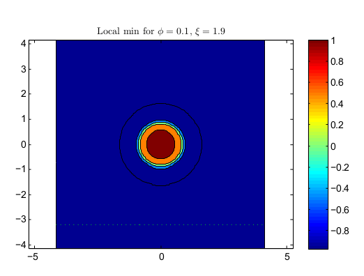
(a) Level curves of the local min for $\phi=0.1$, $\xi=1.9$.

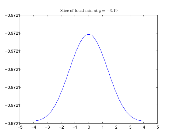
(b) Cross-section of the local min at $y=-3.19$.

Figure 3.1: The local minimizer has the expected properties. The string is converged with error of order $1e-5$.

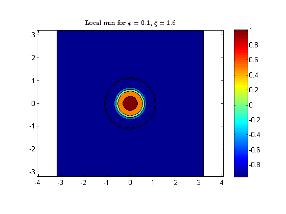
(a) Local minimizer.

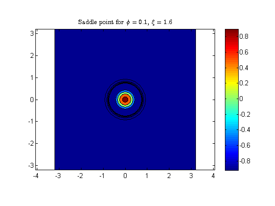
(b) Saddle point.

Figure 3.2: Local minimizer and saddle point for $\phi=0.1$ and $\xi=1.6$, i.e., in the regime that the constant state is not the global minimizer. The string is converged up to error $1e-5$.

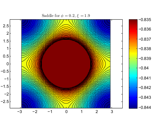
Figure 3.3: A close-up of the level lines of the saddle point for $\phi=0.2$ and $\xi=1.9$. The string is converged up to error $1e-4$. This figure motivates the analysis in section 4.

4 Convexity

In the following sections we consider the volume-constrained minimizers; that is, we consider the minimizers of the energy (1.1) over the set

$$X_{\phi,\omega}:=\left\{u\in H^{1}\cap L^{4}(\mathbb{T}_{\phi L}):\mathchoice{{\vbox{\hbox{$\textstyle-$}}\kern-4.86108pt}}{{\vbox{\hbox{$\scriptstyle-$}}\kern-3.25pt}}{{\vbox{\hbox{$\scriptscriptstyle-$}}\kern-2.29166pt}}{{\vbox{\hbox{$\scriptscriptstyle-$}}\kern-1.875pt}}\!\int_{\mathbb{T}_{\phi L}}u\,dx=-1+\phi,\quad\nu(u)=\omega\right\},$$ (4.1)

where the “volume” $\nu(\cdot)$ is given by (1.4). We are interested in geometric properties of the minimizers. For simplicity of notation, we will write $u$ instead of $u_{\omega,\phi}$.

We would like to understand convexity of the superlevel sets of the constrained minimizers. Based on the numerics (see for instance Figure 3.3), it seems likely that the superlevel sets are convex not only near the maximum but for all values up to some critical value, at which point the convexity changes and the sublevel sets around the minimum become convex. Such a result is currently out of reach, but we will adapt a method of Caffarelli and Spruck to demonstrate convexity of superlevel sets under Hypothesis (H2), below. Before turning to this result, we recall some basic facts from the previous analysis.

We begin by recalling two results from [GWW] and [GWW20]. We recall first that, according to the mean condition, the definition of $\nu(\cdot)$, and Lemma 2.9 from [GWW], one has the following uniform bounds.

Lemma 4.1.

For any $\omega_{1}>0$ there exists $\phi_{0}>0$ such that for all $\phi\in(0,\phi_{0})$, any volume-constrained minimizer $u$ for $\omega\in[\omega_{1},\xi^{3}/2]$ satisfies

$$-1-\phi^{1/3}\leq\inf_{\mathbb{T}_{\phi L}}u\leq-1+\phi\leq 1-2\phi^{1/3}\leq\sup_{\mathbb{T}_{\phi L}}u\leq 1+\phi^{1/3}.$$ (4.2)

The upper bound $\phi_{0}$ from Lemma 4.1 is the only restriction we will place on $\phi>0$ for the rest of the article. As a consequence of the uniform bounds, any constrained minimizer is smooth and satisfies the Euler Lagrange equation

$$-\phi\Delta u+\frac{1}{\phi}G^{\prime}(u)+\lambda_{\phi}+\lambda_{\omega}\chi^{\prime}(u)=0\qquad\hbox{in}\>\mathbb{T}_{\phi L},$$ (4.3)

where $\lambda_{\phi}$, $\lambda_{\omega}\in\mathbb{R}$ are Lagrange parameters corresponding to the mean and volume constraints, respectively. Next we recall the symmetry of the constrained minimizers.

Theorem 4.2 (Theorem 1.1, [GWW20]).

Any volume-constrained minimizer $u$ is equal (up to a translation) to its Steiner symmetrization about the origin. In particular, its superlevel sets are simply connected, and $u$ is strictly decreasing along all rays starting at the (unique) maximum of $u$. In fact for any ray $e$ starting in the maximum, the directional derivative is strictly negative:

$$\partial_{e}u<0$$ (4.4)

on all of $\{x\in\mathbb{T}_{\phi L}:x_{i}>0,\,i=1,\ldots,d\}$ and the gradient vanishes only at the (unique) maximum and minimum.

Remark 4.3.

The first part of the theorem is precisely Theorem 1.1 from [GWW20], and (4.4) and the nonvanishing of the gradient follow from the Strong Maximum Principle, as shown in the proof of Theorem 1.1 in [GWW20].

4.1 Adaptation of a method of Caffarelli and Spruck

We will now use the Euler Lagrange equation (4.3) and a method that Caffarelli and Spruck introduced in [CS, Theorem 2.1] to establish convexity of the superlevel sets of volume-constrained minimizers $u=u_{\omega,\phi}$ under an assumption on the nonlinearity, specified in Hypothesis (H2), below. We assume without loss of generality that the location of the unique maximum of $u$ is $x=0$. By symmetry it is often sufficient to restrict to the first quadrant, i.e., to

$$\mathbb{T}_{\phi L}^{+}:=\{x\in\mathbb{T}_{\phi L}:x_{i}>0,\,i=1,\ldots,d\}.$$

Remark 4.4.

By symmetry of $u$ we have for $i\neq j$ that

$$\partial_{i}u(0,\ldots,0,x_{j},0,\ldots,0)=0.$$

Hence the Hessian matrix $D^{2}u(0)$ is diagonal, and we have

$$\left(D^{2}u(0)\right)_{ij}=\lambda_{i}\delta_{ij}$$

where $(\delta_{ij})_{ij}$ denotes the identity matrix in $\mathbb{R}^{d}$ and $\lambda_{i}\in\mathbb{R}$ for $i\in\{1,\ldots,d\}$. Because $x=0$ is a maximum point of $u$, we have $\lambda_{i}\leq 0$ for $i\in\{1,\ldots,d\}$. More is true:

Lemma 4.5.

The origin is a non-degenerate critical point of any volume-constrained minimizer $u$, and $\partial^{2}_{e}u(0)<0$ for any ray $e$ starting in the origin.

Proof.

Let $e$ be any ray starting in the origin. We choose $i\in\{1,\ldots,d\}$ such that $e$ points into the halfspace $\mathbb{T}_{\phi L}^{i}:=\{x\in\mathbb{T}_{\phi L}:x_{i}>0\}$. According to Theorem 4.2, we have $\partial_{e}u<0$ in $\mathbb{T}_{\phi L}^{i}$. Note that by (4.3) the function $\partial_{e}u$ satisfies the equation

$$-\phi\Delta(\partial_{e}u)+\left(\frac{1}{\phi}G^{\prime\prime}(u)+\lambda_{\omega}\>\chi^{\prime\prime}(u)\right)\partial_{e}u=0\qquad\text{in $\mathbb{T}_{\phi L}^{i}$. }$$

For any $\rho>0$ such that ball $B_{\rho}(0)\Subset\mathbb{T}_{\phi L}$, the function $\partial_{e}u$ takes its maximum in $\overline{\mathbb{T}_{\phi L}^{i}\cap B_{\rho}(0)}$ in $x=0$. Hence Hopf’s maximum principle yields $\lambda=\partial^{2}_{e}u(0)<0$. Consequently $x=0$ is a non-degenerate maximum point. ∎

As a consequence of Lemma 4.5, the superlevel sets $S_{c}:=\{u>c\}$ are strictly convex for all $c$ sufficiently close to $u_{max}:=\sup_{\mathbb{T}_{\phi L}}u$, which according to (4.2) is close to $1$. Thus there exists $c^{*}<u_{max}$ such that $S_{c}$ is convex for all $c^{*}\leq c<u_{max}$.

We would now like to investigate convexity of superlevel sets of $u$ further away from $u_{max}$. Suppose that $c_{*}>\inf_{\mathbb{T}_{\phi L}}u$ is some value such that

Hypothesis (H1):

$$S_{c_{*}}=\{u>c_{*}\}\text{ is convex and }\partial S_{c_{*}}\text{ is smooth.}$$

We assume that $c^{*}>c_{*}$ since otherwise there is nothing to prove. We will show that all sublevel sets $S_{c}$ for $c_{*}<c<c^{*}$ are convex.

In the remainder of this section we will write the Euler-Lagrange equation of $u$ in the form $\Delta u=f(u)$, where

$$f(u):=\frac{1}{\phi^{2}}G^{\prime}(u)+\frac{\lambda_{\phi}}{\phi}+\frac{\lambda_{\omega}}{\phi}\chi^{\prime}(u).$$ (4.5)

Note that because of the smoothness of $G$ and $\chi$, $f$ is also smooth. We will work under the assumption:

Hypothesis (H2):

$$f(c)>0\quad\text{and}\quad f^{\prime}(c)>0\quad\hbox{for all}\quad c_{*}<c<u_{max}.$$

In the sequel we will work with three collinear points $x,y,z\in S_{c_{*}}$ such that $z=tx+(1-t)y$ for some $t\in(0,1)$, and we will write $z\in[x,y]$ for short and speak of “the triple” $(x,y,z)$. We will call a triple admissible if it is an element of

$${\cal{A}}:=\{(x,y,z)\colon x,y,z\>\hbox{are collinear},\>x,y\in S_{c_{*}},\text{and }\>u(x)>u(z)\}.$$ (4.6)

Note that ${\cal{A}}$ is not empty since $u$ is strictly decreasing along all rays emanating from the origin.

We consider the function

$$F(x,y,z):=u(y)-u(z),\qquad\hbox{for}\quad(x,y,z)\in{\cal{A}}.$$

Because of the equivalence in Lemma 4.6 below, we will be interested in

$$\sup_{(x,y,z)\in{\cal{A}}}F(x,y,z).$$

Let $(x_{k},y_{k},z_{k})\in{\cal{A}}$ be a maximizing sequence for $F$. By compactness of $\overline{S_{c_{*}}}$, there exist limit points $x_{0},y_{0},z_{0}\in\overline{S_{c_{*}}}$. By passing to suitable subsequences, we may assume that $x_{k}\to x_{0}$, $y_{k}\to y_{0}$ and $z_{k}\to z_{0}$. Moreover $z_{0}=t_{0}x_{0}+(1-t_{0})y_{0}$ for some $t_{0}\in[0,1]$ and $u(x_{0})\geq u(z_{0})$. A priori it may be that $x_{0}=z_{0}$ or $z_{0}=y_{0}$ or even $x_{0}=z_{0}=y_{0}$, however see Remark 4.8.

Our plan in order to show convexity of $S_{c}=\{u>c\}$ for all $c_{*}<c<u_{max}$ is as follows.

• In Lemma 4.6, we show that convexity of $S_{c}$ for all $c_{*}<c<u_{max}$ is equivalent to

  $$\sup_{(x,y,z)\in{\cal{A}}}F(x,y,z)\leq 0.$$

• We then argue by contradiction. Thus we assume that $\sup_{(x,y,z)\in{\cal{A}}}F(x,y,z)>0$ and derive necessary conditions for the limit $(x_{0},y_{0},z_{0})$ of the maximizing sequence (see Lemmas 4.9 - 4.13). The proofs rely heavily on Lemma 4.5, however they do not explicitly use the equation for $u$. In particular (H2) is not needed.

• The main result of this section is Proposition 4.14. It states that if $S_{c_{*}}$ is convex, then the superlevel sets $S_{c}$ are convex for all $c_{*}<c<u_{max}$. It is only now that Hypothesis (H2) is needed. The main part of the proof is based on a domain variation argument. Specifically, using that $(x_{0},y_{0},z_{0})$ is extremal, we perform a variation in the independent variables, using Lemmas 4.9 - 4.13 to show that the perturbed point $(x^{*}_{0},y^{*}_{0},z^{*}_{0})$ satisfies

  $$F(x^{*}_{0},y^{*}_{0},z^{*}_{0})>F(x_{0},y_{0},z_{0})>0,$$

  which violates the extremality of $(x_{0},y_{0},z_{0})$.

Lemma 4.6.

The convexity of $S_{c}$ for all $c_{*}\leq c\leq u_{max}$ is equivalent to

$$\sup_{(x,y,z)\in{\cal{A}}}F(x,y,z)\leq 0.$$ (4.7)

Proof.

Step 1. We begin by assuming that the sets $S_{c}$ are convex for all $c_{*}<c<u_{max}$. Let $(x,y,z)\in{\cal{A}}$. If $u(y)>u(x)$, then convexity of the superlevel sets gives $u(z)\geq u(x)$ for all $z\in[x,y]$ and $(x,y,z)$ is not admissible. Hence any admissible triple satisfies $u(x)\geq u(y)$. However then the convexity of the superlevel sets gives $u(z)\geq u(y)$, so that $F(x,y,z)\leq 0$, and taking the supremum over ${\cal{A}}$ preserves this inequality.
Step 2. We now assume $\sup_{(x,y,z)\in{\cal{A}}}F(x,y,z)\leq 0$ and will show that $S_{c}$ is convex for all $c_{*}<c<u_{max}$. Let $x,y\in S_{c}$. For any $z\in[x,y]$, if $(x,y,z)$ is admissible, then our assumption on $F$ yields $u(z)\geq u(y)>c$. On the other hand if $z\in[x,y]$ and $(x,y,z)$ is not admissible, then by definition of the admissible set there holds $u(z)\geq u(x)>c$. Hence in either case $z\in S_{c}$, and thus $S_{c}$ is convex. ∎

In order to prove the convexity of $S_{c}$ for all $c_{*}\leq c\leq u_{max}$, we will use Lemma 4.6 and argue by contradiction. Thus we assume that (4.7) does not hold and we will discuss the extremal situation, by which we mean the following:

Definition 4.7.

We will call $(x_{0},y_{0},z_{0})$ a positive extremal if there exists a maximizing sequence $(x_{k},y_{k},z_{k})\in{\cal{A}}$ with $x_{k}\to x_{0}$, $y_{k}\to y_{0}$ and $z_{k}\to z_{0}$ such that

• $x_{0},y_{0},z_{0}\in\overline{S_{c_{*}}}$ and $z_{0}=t_{0}x_{0}+(1-t_{0})y_{0}$ for some $t_{0}\in[0,1]$;

• $u(x_{0})\geq u(z_{0})$;

• there holds $0<\sup_{(x,y,z)\in{\cal{A}}}F(x,y,z)=F(x_{0},y_{0},z_{0})$, so that

  $$u(y_{0})>u(z_{0}).$$ (4.8)

Remark 4.8.

Clearly for any positive extremal there holds $x_{0}\neq y_{0}$, since otherwise $x_{0}=y_{0}=z_{0}$ (by ($P_{1}$)), which would imply $F(x_{0},y_{0},z_{0})=0$ and hence violate ($P_{3}$). Also $y_{0}\neq z_{0}$ (i.e., $t_{0}\neq 0$), since this would also imply $F(x_{0},y_{0},z_{0})=0$. On the other hand, the case $x_{0}=z_{0}$ cannot be excluded. (Indeed, Lemma 4.12 shows that this equality holds for any positive extremal if $f$ is analytic.)

Lemma 4.9.

If the triple $(x_{0},y_{0},z_{0})$ is a positive extremal, then $y_{0}\neq 0$.

Proof.

For a contradiction we consider any triple $(x_{0},y_{0},z_{0})$ with $y_{0}=0$, i.e., $y_{0}$ is the unique point where $u$ takes its maximum. We will show that $(x_{0},y_{0},z_{0})$ is not the limit of a sequence of admissible triples $(x_{k},y_{k},z_{k})\in{\cal{A}}$ as $k\to\infty$. Thus assume that there exists a sequence $(x_{k},y_{k},z_{k})\in{\cal{A}}$ such that $\lim_{k\to\infty}(x_{k},y_{k},z_{k})=(x_{0},y_{0},z_{0})$. We distinguish the following cases.

• If $y_{0}=0$ and $x_{0}\neq z_{0}$, then by ($P_{1}$), we have $z_{0}=t_{0}x_{0}$ for some $t_{0}\in(0,1]$. Since by Lemma 4.5), $u$ is strictly decreasing along any ray starting in the origin, there holds $u(z_{0})>u(x_{0})$, which contradicts (P2).

• Now suppose $y_{0}=0$ and $x_{0}=z_{0}$. Because $(x_{k},y_{k},z_{k})$ is admissible, we have $u(x_{k})>u(z_{k})$. From the collinearity of $(x_{0},y_{0},z_{0})$ and $y_{0}=0$, we deduce that

  $$\frac{x_{k}-z_{k}}{|x_{k}-z_{k}|}=\frac{x_{k}-y_{k}}{|x_{k}-y_{k}|}\to\frac{x_{0}}{|x_{0}|}=:e_{0}\quad\text{as $k\to\infty$.}$$

  Hence

  $$0<\frac{u(x_{k})-u(z_{k})}{|x_{k}-z_{k}|}=\int\limits_{0}^{1}\frac{x_{k}-z_{k}}{|x_{k}-z_{k}|}\cdot Du(sx_{k}+(1-s)z_{k})\>ds\to e_{0}\cdot Du(x_{0})=\partial_{e_{0}}u(x_{0}),$$

  and we obtain in the limit $k\to\infty$ that $\partial_{e_{0}}u(x_{0})\geq 0,$ which contradicts the fact that the directional derivative is strictly negative along rays from the origin (cf. Theorem 4.2).

∎

Lemma 4.10.

For any positive extremal $(x_{0},y_{0},z_{0})$, there holds

• $y_{0}\in S_{c_{*}}$ and

• $z_{0}\in S_{c_{*}}$.

Proof.

Since necessarily $y_{0},z_{0}\in\overline{S_{c_{*}}}$, the issue is to show $y_{0},z_{0}\notin\partial S_{c_{*}}$. We begin by considering $y_{0}$. Since $z_{0}\in\overline{S_{c_{*}}}$, we have $u(z_{0})\geq c_{*}$. Combining this with (4.8) implies (i).

We now turn to $z_{0}$. Let us assume $z_{0}\in\partial S_{c_{*}}$, i.e., $u(z_{0})=c_{*}$. By (i) we have $y_{0}\in S_{c_{*}}$. By ($P_{1}$) the points $x_{0}$, $y_{0}$ and $z_{0}$ are collinear. Since $S_{c_{*}}$ is convex, the ray that starts in $y_{0}$ and passes through $z_{0}$ and $x_{0}$ intersects $\partial S_{c_{*}}$ in exactly one point. By ($P_{1}$) and ($P_{2}$) the point $x_{0}$ must be in $\partial S_{c_{*}}$ and thus $x_{0}=z_{0}$. Now let $(x_{k},y_{k},z_{k})\in{\cal{A}}$ be a maximizing sequence converging to $(x_{0},y_{0},z_{0})$ as in Definition 4.7. For sufficiently large $k$ the following holds: Since $x_{k},z_{k}\to x_{0}=z_{0}\in\partial S_{c_{*}}$, there exists - for $k$ large - a ray that starts in $y_{k}$, passes through $z_{k}$ and $x_{k}$ and intersects $\partial S_{c_{*}}$ in exactly one point. This point is denoted by $\tilde{x}_{k}$. Note that $x_{k}\in[\tilde{x}_{k},z_{k}]$ and $\tilde{x}_{k}\to x_{0}$ as $k\to\infty$. Since $\partial S_{c_{*}}$ is smooth, Hopf’s boundary lemma applied on $S_{c_{*}}$ then implies that $u$ is strictly increasing along $[\tilde{x}_{k},z_{k}]$ (for $k$ large enough). However then $u(x_{k})<u(z_{k})$ which contradicts the admissibility of $(x_{k},y_{k},z_{k})$. As a consequence $z_{0}\notin\partial S_{c_{*}}$. ∎

Here and below, let

$$e:=\frac{x_{0}-y_{0}}{|x_{0}-y_{0}|}$$ (4.9)

be the unit vector pointing from $y_{0}$ to $x_{0}$.

Lemma 4.11.

For any positive extremal $(x_{0},y_{0},z_{0})$, there holds $\partial_{e}u(z_{0})=0$.

Proof.

We consider separately the cases $x_{0}\neq z_{0}$ and $x_{0}=z_{0}$. If $x_{0}\neq z_{0}$, then according to ($P_{1}$) and ($P_{3}$), $u$ has a minimum in $z_{0}$ along the segment $[x_{0},y_{0}]$, which implies $\partial_{e}u(z_{0})=0$. If $x_{0}=z_{0}$, then ($P_{1}$), ($P_{3}$), and the definition of ${\cal{A}}$ imply that for any maximizing sequence $(x_{k},y_{k},z_{k})\in{\cal{A}}$, the function $u$ has an interior minimum at some point $\xi_{k}$ between $y_{k}$ and $x_{k}$, so that $\partial_{e}u(\xi_{k})=0$. Necessarily $\xi_{k}$ converges to some point $\xi_{0}\in[y_{0},x_{0}]$. If $\xi_{0}$ lies in the interior, then minimality of $z_{0}=x_{0}$ is contradicted. Hence $\xi_{0}=x_{0}=z_{0}$ and $\partial_{e}u(z_{0})=0$. ∎

Lemma 4.12.

For any positive extremal $(x_{0},y_{0},z_{0})$, there holds (i) $\partial_{e}u(y_{0})=0$, (ii) $x_{0}=z_{0}$ or $u$ is constant on $[x_{0},z_{0}]$, and (iii) $\partial_{e}^{2}u(z_{0})=0$.

Proof.

ad (i). From Lemma 4.10 we know that $y_{0}\in S_{c_{*}}$. We consider perturbing $F$ by varying $y_{0}$ in the $e$ direction: Let $y_{0}^{s}$ be given by

$$y_{0}^{s}=y_{0}+s\>e\quad\hbox{where}\quad|s|<s_{0}$$ (4.10)

for $s_{0}>0$ small enough that $y_{0}^{s}\in S_{c_{*}}$ and $y_{0}^{s}\neq z_{0}$ for all $|s|<s_{0}$. Then

$$F(x_{0},y_{0},z_{0})\geq F(x_{0},y_{0}^{s},z_{0})$$ (4.11)

for all $|s|<s_{0}$, which implies $\partial_{e}u(y_{0})=0$.

ad (ii). It suffices to assume that $x_{0}\neq z_{0}$ and show that $u$ is constant on the segment $[x_{0},z_{0}]$. We know that $u(x_{0})\geq u(z_{0})$ (this is ($P_{2}$)). If $u$ is not constant along the segment $[x_{0},z_{0}]$, then there exists an intermediate point $\tilde{x}$ between $x_{0}$ and $z_{0}$ such that $u(\tilde{x})\neq u(z_{0})$, and necessarily $u(\tilde{x})>u(z_{0})$, since otherwise $(x_{0},y_{0},\tilde{x})$ is admissible and $u(y_{0})-u(\tilde{x})>u(y_{0})-u(z_{0})$, violating optimality of the triple $(x_{0},y_{0},z_{0})$. We now consider the triple $(\tilde{x},y_{0},z_{0})$. Since the points are collinear and $u(\tilde{x})>u(z_{0})$, this triple is admissible, and since $F(\tilde{x},y_{0},z_{0})=F(x_{0},y_{0},z_{0})$, $(\tilde{x},y_{0},z_{0})$ is a positive extremal, as well. As in Step 1, we deduce $F(\tilde{x},y_{0},z_{0})\geq F(\tilde{x},y_{0}^{s},z_{0})$ for all sufficiently small perturbations in the $e$ direction. Next we rotate the segment $[\tilde{x},y_{0}]$ about an angle $\theta$ with center $z_{0}$. Letting $X$ denote the rotation of $\tilde{x}$, we observe that $u(X)>u(z_{0})$ if $\theta$ is small enough. Let $Y_{0}$ denote the rotation of $y_{0}$. For $\theta$ small enough $Y_{0}\notin\partial S_{c_{*}}$ and the triple $(X,Y_{0},z_{0})$ is admissible (see Figure 4.1). Since $(\tilde{x},y_{0},z_{0})$ is a positive extremal, we have (for all $\theta$ small enough) that

$$F(\tilde{x},y_{0},z_{0})\geq F(X,Y_{0},z_{0})>0.$$ (4.12)

Note that all points in a sufficiently small neighbourhood of $y_{0}$ can be described as a perturbation of $y_{0}$ in the direction $e$ combined with a rotation about a small angle $\theta$. Hence combining shifts and rotations allows us to deduce that $u$ has a local maximum in $y_{0}$. This is impossible, since $y_{0}\neq 0$ by Lemma 4.9 and since by Theorem 4.2 $u$ is strictly decreasing on all rays from the origin. From this contradiction we deduce that if $x_{0}\neq z_{0}$, then $u$ is constant along the segment $[z_{0},x_{0}]$.

ad (iii). Recall from Lemma 4.11 that $\partial_{e}u(z_{0})=0$. Optimality of the triple hence implies $\partial_{e}^{2}u(z_{0})\geq 0$. Strict inequality $\partial_{e}^{2}u(z_{0})>0$ would however allow us to combine shifts as in (4.10) and rotations around $z_{0}$ in order to deduce (similarly to in Step 2 above) that $u$ has a local maximum in $y_{0}$, which, as in Step 2, can be ruled out. Hence $\partial_{e}^{2}u(z_{0})=0$. ∎

Figure 4.1:

Lemma 4.13.

For any positive extremal, $|\nabla u(y_{0})|\neq 0$, $|\nabla u(z_{0})|\neq 0$, and there holds

$$\frac{\nabla u(z_{0})}{|\nabla u(z_{0})|}=\frac{\nabla u(y_{0})}{|\nabla u(y_{0})|}.$$ (4.13)

Proof.

The nonvanishing of the gradient in $y_{0}$ and $z_{0}$ follows from Theorem 4.2, Lemmas 4.9 and 4.10, and $c_{*}>u_{min}$. Now assume that (4.13) does not hold. Then there exists a vector $v\in\mathbb{R}^{d}$ such that

$$v\cdot\nabla u(y_{0})>0\qquad\hbox{and}\qquad v\cdot\nabla u(z_{0})<0.$$ (4.14)

Step 1. By Lemma 4.12 we have $u(x_{0})=u(z_{0})$ in the positive extremal case. We will now construct an admissible triple that we will then use in Step 3 to contradict extremality. We begin by writing $y_{0}=z_{0}+|y_{0}-z_{0}|\hat{e}$, for the unit vector

$$\hat{e}:=\frac{y_{0}-z_{0}}{|y_{0}-z_{0}|}$$

pointing from $z_{0}$ to $y_{0}$. For $\epsilon>0$ we perturb $y_{0}$ and consider the set

$$\left\{w_{t}:=z_{0}+(1-t)|y_{0}-z_{0}|\hat{e}+(1-t)\,\epsilon v\>:\>t\in(0,1)\right\}.$$

The above set includes a segment joining $w_{0}=y_{0}+\epsilon v$ (for $t=0$) and $w_{1}=z_{0}$ (for $t=1$). For $t=0$ we observe that

$$\left(w_{0}-y_{0}\right)\cdot\nabla u(y_{0})=\epsilon v\cdot\nabla u(y_{0})\overset{\eqref{convex41}}{>}0.$$

On the other hand for all $t\in[0,1)$ there holds

$$\left(w_{t}-z_{0}\right)\cdot\nabla u(z_{0}) = (1-t)(y_{0}-z_{0})\cdot\nabla u(z_{0})+(1-t)\epsilon v\cdot\nabla u(z_{0})$$

$$= (1-t)\epsilon v\cdot\nabla u(z_{0})\overset{\eqref{convex41}}{<}0,$$

where the second equality holds because of Lemma 4.11. For small $t_{0}>0$ we now consider the triple $(w_{1+t_{0}},w_{0},w_{1-t_{0}})$. To see that this triple is admissible for $\epsilon$ and $t_{0}$ close to zero, it suffices to check:

• For $t=\frac{1-t_{0}}{1+t_{0}}\in(0,1)$ we have $w_{1-t_{0}}=tw_{1+t_{0}}+(1-t)w_{0}$. Thus the three points are collinear.

• Since $u(x_{0})=u(z_{0})$ (according to Lemma 4.12) and both $z_{0}$ and $y_{0}$ lie in the interior of $S_{c_{*}}$ (by Lemma 4.10), there holds $w_{1+t_{0}},\,w_{0}\in S_{c_{*}}$ for $t_{0}$ and $\epsilon$ sufficiently small.

• Expanding $u(w_{1+t_{0}})-u(w_{1-t_{0}})$ with respect to $t_{0}$ and $\epsilon$ and applying Lemma 4.11, there holds $u(w_{1+t_{0}})>u(w_{1-t_{0}})$ for $t_{0}$ and $\epsilon$ sufficiently small.

Hence for $t_{0}$ and $\epsilon$ sufficiently small, there holds $(w_{1+t_{0}},w_{0},w_{1-t_{0}})\in{\cal{A}}$.

Step 2. We will now contradict the extremality of $(x_{0},y_{0},z_{0})$ by showing that $F(w_{1+t_{0}},w_{0},w_{1-t_{0}})>F(x_{0},y_{0},z_{0})$. Indeed, again using Lemma 4.11, we deduce:

$$F(w_{1+t_{0}},w_{0},w_{1-t_{0}})-F(x_{0},y_{0},z_{0}) = u(w_{0})-u(w_{1-t_{0}})-\left(u(y_{0})-u(z_{0})\right)$$

$$= u(y_{0})+\epsilon v\cdot\nabla u(y_{0})-\left(u(z_{0})+t_{0}\epsilon v\cdot\nabla u(z_{0})\right)+o(\epsilon)$$

$$\qquad-\left(u(y_{0})-u(z_{0})\right)$$

$$= \epsilon\left(v\cdot\nabla u(y_{0})-t_{0}\epsilon v\cdot\nabla u(z_{0})\right)+o(\epsilon).$$

From (4.14) and $t_{0}>0$ we deduce $F(w_{1+t_{0}},w_{0},w_{1-t_{0}})>F(x_{0},y_{0},z_{0})$ for $\epsilon$ small. ∎

Proposition 4.14.

Let $u$ be a Steiner symmetric solution of $\Delta u=f(u)$ in $\mathbb{T}_{\phi L}$, where $f$ is given by (4.5). Assume $u$ takes its unique maximum point $u_{max}$ in $x=0$. Let $c_{*}<u_{max}$ be a level such that Hypotheses (H1) and (H2) hold. Then $S_{c}$ is convex for all $c_{*}<c<u_{max}$.

Proof.

We argue by contradiction. Thus we assume that there exists a $c\in(c_{*},u_{max})$ such that $S_{c}$ is not convex. By Lemma 4.6 this is equivalent to

$$\sup_{(x,y,z)\in{\cal{A}}}F(x,y,z)>0.$$

Let $(x_{0},y_{0},z_{0})$ be a positive extremal. Once again the idea is to perturb $y_{0}$ and $z_{0}$ to construct an admissible triple that contradicts optimality of $(x_{0},y_{0},z_{0})$. This is done in several steps.

Step 1. We begin by making the strategy more precise. For smooth maps $\Phi,\hat{\Phi}:\mathbb{T}_{\phi L}\to\mathbb{T}_{\phi L}$ with $\Phi(0)=\hat{\Phi}(0)=0$ we define

$$u_{1}(x):=u(y_{0}+\Phi(x))\qquad\text{and}\qquad u_{2}(x):=u(z_{0}+\hat{\Phi}(x)).$$

Next we set

$$v(x):=u_{1}(x)-u_{2}(x)-(u(y_{0})-u(z_{0})).$$ (4.15)

and

$$w(x):=\left(\nabla u\right)(z_{0}+\hat{\Phi}(x))\cdot\left(z_{0}+\hat{\Phi}(x)-(y_{0}+\Phi(x))\right).$$ (4.16)

We will find conditions on $\Phi$ and $\hat{\Phi}$ that imply:

1. There exists $r>0$ such that $v(x)>0$ in $B_{r}(0)\setminus\{0\}$.

2. For any $r>0$ sufficiently small, there exists at least one point $\tilde{x}\in B_{r}(0)$ such that $w(\tilde{x})>0$.

We will use these facts to deduce that

$$y_{*}:=y_{0}+\Phi(\tilde{x}),\quad z_{*}:=z_{0}+\hat{\Phi}(\tilde{x}),\qquad x_{*}:=(1+\varepsilon)z_{*}-\varepsilon y_{*}$$

for $\varepsilon>0$ small define an admissible triple and $F(x_{*},y_{*},z_{*})>F(x_{0},y_{0},z_{0})$, contradicting the extremality of $(x_{0},y_{0},z_{0})$. Clearly $v(\tilde{x})>0$ implies the latter inequality, so it suffices to check the admissibility. Appropriate collinearity follows from

$$z_{*}=\frac{1}{1+\varepsilon}x_{*}+\frac{\varepsilon}{1+\varepsilon}y_{*}\qquad\text{for }\varepsilon\in(0,1).$$

Also $\Phi(0)=\hat{\Phi}(0)=0$ and that $z_{0}$, $y_{0}$ lie in the interior of $S_{c_{*}}$ (again by Lemma 4.10) yield $x_{*},\,y_{*}\in S_{c_{*}}$ for $|x|$ and $\varepsilon$ small enough. Finally we remark that $u(x_{*})>u(z_{*})$ for $\varepsilon$ sufficiently small if $w(\tilde{x})>0$. Hence it remains only to verify the above claims (i) and (ii) for $w$ and $v$.

Step 2. We will now use Taylor expansions to find appropriate conditions on $\Phi$ and $\hat{\Phi}$. For $v$ near the origin we obtain

$$v(x) = x\cdot\left(D\Phi(0)\,\nabla u(y_{0})\right)-x\cdot\left(D\hat{\Phi}(0)\,\nabla u(z_{0})\right)$$

$$+\frac{1}{2}\>\partial_{i}u(y_{0})\,\left(D^{2}\Phi_{i}(0)\,x\right)\cdot x-\frac{1}{2}\>\partial_{i}u(z_{0})\,\left(D^{2}\hat{\Phi}_{i}(0)\,x\right)\cdot x$$

$$+\frac{1}{2}\,\cdot\left(D^{2}u(y_{0})\,\left(D\Phi(0)x\right)\right)\cdot\left(D\Phi(0)x\right)-\frac{1}{2}\,\cdot\left(D^{2}u(y_{0})\,\left(D\hat{\Phi}(0)x\right)\right)\cdot\left(D\hat{\Phi}(0)x\right)$$

$$+o(|x|^{2}),$$

where we sum over repeated indices and $\frac{o(|x|^{2})}{|x|^{2}}\to 0$ as $|x|\to 0$. Similarly for $w$ we get

$$w(x) = \partial_{i}u(z_{0})\,\left(D\left(\hat{\Phi}_{i}-\Phi_{i}\right)(0)\,x\right)+\left(D^{2}u(z_{0})\,\left(D\hat{\Phi}(0)\,x\right)\right)\cdot(z_{0}-y_{0})$$

$$+\frac{1}{2}\,\partial_{i}u(z_{0})\,\left(D^{2}\left(\hat{\Phi}_{i}-\Phi_{i}\right)(0)\,x\right)\cdot x+\left(D^{2}u(z_{0})\,\left(D\hat{\Phi}(0)x\,\right)\right)\cdot\left(D(\hat{\Phi}-\Phi)(0)\,x\right)$$

$$+\frac{1}{2}\,\left(D^{2}\hat{\Phi}_{i}(0)\,x\right)\cdot x\>\partial_{i}\partial_{j}u(z_{0})\,(z_{0}-y_{0})_{j}+\frac{1}{2}\,(z_{0}-y_{0})_{i}\,\left(D^{2}\partial_{i}u(z_{0})\,\left(D\hat{\Phi}(0)x\right)\right)\cdot\left(D\hat{\Phi}(0)x\right)$$

$$+o(|x|^{2}).$$

Our goal is to choose the coefficients of the Taylor expansion of $\Phi$ and $\hat{\Phi}$ such that for some $\mu>0$ and some $r>0$, there holds

$$v(x)\geq\mu|x|^{2}\quad\hbox{in}\>B_{r}(0)\qquad\hbox{and}\qquad w(x)>0\>\hbox{for at least one}\>x\in{B_{r}(0)}.$$ (4.19)

Setting

$$a:=\frac{1}{|\nabla u(y_{0})|}\qquad\text{and}\qquad b:=\frac{1}{|\nabla u(z_{0})|},$$

we will show that it suffices to choose $\Phi$ and $\hat{\Phi}$ so that $D\Phi(0)_{ij}=a\,\delta_{ij}$ and $D\hat{\Phi}(0)_{ij}=b\,\delta_{ij}.$ Note that Lemma 4.13 implies

$$x\cdot\left(D\Phi(0)\,\nabla u(y_{0})\right)-x\cdot\left(D\hat{\Phi}(0)\,\nabla u(z_{0})\right)=a\,x\cdot\nabla u(y_{0})-b\,x\cdot\nabla u(z_{0})=0,$$

so that (4.1) and (4.1) improve to

$$v(x) = \frac{1}{2}\>\partial_{i}u(y_{0})\,\left(D^{2}\Phi_{i}(0)\,x\right)\cdot x-\frac{1}{2}\>\partial_{i}u(z_{0})\,\left(D^{2}\hat{\Phi}_{i}(0)\,x\right)\cdot x$$

$$+\frac{a^{2}}{2}\,\left(D^{2}u(y_{0})\,x\right)\cdot x-\frac{b^{2}}{2}\,\left(D^{2}u(y_{0})\,x\right)\cdot x+o(|x|^{2}),$$

and

$$w(x) = (b-a)\,x\cdot\nabla u(z_{0})+b\,\left(D^{2}u(z_{0})\,x\right)\cdot(z_{0}-y_{0})$$

$$+\frac{1}{2}\,\partial_{i}u(z_{0})\,\left(D^{2}\left(\hat{\Phi}_{i}-\Phi_{i}\right)(0)\,x\right)\cdot x+b(b-a)\,\left(D^{2}u(z_{0})\,x\right)\cdot x$$

$$+\frac{1}{2}\>\partial_{i}\partial_{j}u(z_{0})\,(z_{0}-y_{0})_{j}\,\left(D^{2}\hat{\Phi}_{i}(0)\,x\right)\cdot x+\frac{b^{2}}{2}\,(z_{0}-y_{0})_{i}\,\left(D^{2}\partial_{i}u(z_{0})\,x\right)\cdot x$$

$$+o(|x|^{2}),$$

respectively.

We set $D^{2}\hat{\Phi}_{i}(0)=0$. In view of (4.19) a natural choice for $D^{2}\Phi(0)$ is then

$$\left(D^{2}\Phi_{i}(0)\right)_{jk}=a\,\partial_{i}u(y_{0})\left(-a^{3}\,\partial_{j}\partial_{k}u(y_{0})+a\,b^{2}\,\partial_{j}\partial_{k}u(z_{0})+4\,a\,\mu\,\delta_{jk}\right).$$

for some $\mu>0$. This implies

$$\frac{1}{2}\>\partial_{i}u(y_{0})\,\left(D^{2}\Phi_{i}(0)\,x\right)\cdot x:=-\frac{a^{2}}{2}\,\left(D^{2}u(y_{0})\,x\right)\cdot x+\frac{b^{2}}{2}\,\left(D^{2}u(z_{0})\,x\right)\cdot x+2\,\mu\,|x|^{2}.$$

Substituting into (4.1) yields $v(x)=2\mu|x|^{2}+o(|x|^{2})$ and hence the first statement in (4.19).

Step 3. It remains to prove the second part of (4.19). From Lemma 4.13 we deduce

$$\frac{1}{2}\>\partial_{i}u(z_{0})\,\left(D^{2}\Phi_{i}(0)\,x\right)\cdot x=-\frac{a^{3}}{2b}\,\left(D^{2}u(y_{0})\,x\right)\cdot x+\frac{a\,b}{2}\,\left(D^{2}u(z_{0})\,x\right)\cdot x+2\,\mu\,\frac{a}{b}\,|x|^{2}.$$

We plug this into (4.1). Rearranging terms gives

$$w(x) = (b-a)\,x\cdot\nabla u(z_{0})+b\,\left(D^{2}u(z_{0})\,x\right)\cdot(z_{0}-y_{0})+\frac{a^{3}}{2b}\,\left(D^{2}u(y_{0})\,x\right)\cdot x$$

$$-\frac{a\,b}{2}\,\left(D^{2}u(z_{0})\,x\right)\cdot x-2\frac{a}{b}\,\mu|x|^{2}+b(b-a)\,\left(D^{2}u(z_{0})\,x\right)\cdot x$$

$$+\frac{b^{2}}{2}\,(z_{0}-y_{0})_{i}\,\left(D^{2}\partial_{i}u(z_{0})\,x\right)\cdot x+o(|x|^{2}),$$

and a straightforward computation yields

$$\Delta w=\frac{a^{3}}{b}\,\Delta u(y_{0})-a\,b\,\Delta u(z_{0})-4d\frac{a}{b}\,\mu+2b(b-a)\,\Delta u(z_{0})+b^{2}\,\Delta\partial_{i}u(z_{0})\,(z_{0}-y_{0})_{i}+o(1).$$

Recall that according to Lemma 4.11, there holds

$$\partial_{i}\Delta u(z_{0})\,(z_{0}-y_{0})_{i}=f^{\prime}(u(z_{0}))\,\nabla u(z_{0})\cdot(z_{0}-y_{0})=0.$$

Thus

$$\Delta w=\frac{a^{3}}{b}\,\Delta u(y_{0})+(2\,b^{2}-3\,a\,b)\,\Delta u(z_{0})-4d\frac{a}{b}\,\mu+o(1).$$ (4.22)

We will now show that $\Delta w>0$ for $\mu$ and $|x|$ small enough. Combining this fact with $w(0)=0$ and the Strong Maximum Principle, we then obtain the second part of (4.19).

We first consider the case $a=b$, in which equation (4.22) yields

$$\Delta w=a^{2}\left(\Delta u(y_{0})-\Delta u(z_{0})\right)-4d\,\mu+o(1)=a^{2}\left(f(u(y_{0}))-f(u(z_{0}))\right)-4d\,\mu+o(1).$$

We use the equation and Hypothesis (H2). Since $u(y_{0})>u(z_{0})$, the strict monotonicity of $f$ implies $f(u(y_{0}))>f(u(z_{0}))$. Hence for $\mu$ and $|x|$ small enough, we get the existence of a constant $c_{0}>0$ such that $\Delta w\geq c_{0}.$

We now consider the case $a\neq b$ and rewrite (4.22) as

$$\Delta w=\frac{a^{3}}{b}\,f(u(y_{0}))+\left(2b^{2}-3\,a\,b\right)\,f(u(z_{0}))-4\,d\,\frac{a}{b}\,\mu+o(1).$$

Again using the strict monotonicity of $f$, we deduce

$$\Delta w \geq \left(\frac{a^{3}}{b}+2\,b^{2}-3\,a\,b\right)\,f(u(z_{0}))-4d\frac{a}{b}\,\mu+o(1)$$

$$= b^{2}\left(\frac{a}{b}+2\right)\,\left(\frac{a}{b}-1\right)^{2}\,f(u(z_{0}))-4d\frac{a}{b}\,\mu+o(1).$$

Since $f(u(z_{0}))>0$ by Hypothesis (H2), we can again choose $\mu$ and $|x|$ small enough so that there exists $c_{0}>0$ such that $\Delta w\geq c_{0}$. ∎

References

Acknowledgements
We thank Eric Vanden–Eijnden for helpful discussions and for encouraging our interaction. Sebastian Scholtes was partially supported by DFG Grant WE 5760/1-1.