Dust-ion-acoustic shock waves in magnetized plasma having super-thermal electrons

Abstract

The propagation of dust-ion-acoustic shock waves (DIASHWs) in a three-component magnetized plasma having inertialess super-thermal electrons, inertial warm positive ions and negative dust grains has been investigated. A Burgers’ equation is derived by employing the reductive perturbation method. Under consideration of inertial warm positive ions and negative dust grains, both positive and negative shock structures are numerically observed in the presence of super-thermal electrons. The effects of oblique angle ($\delta$), spectral index ($\kappa$), kinematic viscosity ($\eta$), number density and charge state of the plasma species on the formation of the DIASHWs are examined. It is found that the positive and negative shock wave potentials increase with the oblique angle. It is also observed that the magnitude of the amplitude of positive and negative shock waves is not affected by the variation of the kinematic viscosity of plasma species but the steepness of the positive and negative shock waves decreases with kinematic viscosity of plasma species. The implications of our findings in space and laboratory plasmas are briefly discussed.

1 Introduction

Dust grains are omnipresent components in most of the astrophysical environments, viz., interstellar clouds [1, 2, 3, 4], circumstellar clouds [5, 6, 7], interplanetary space [8, 9, 10], Earth’s magnetosphere [11], Saturn’s B ring [12] and magnetosphere [13, 14], Jupiter’s magnetosphere [14, 15], cometary tails [16, 17], and also in laboratory plasmas [18, 19]. In a realistic dusty plasma medium (DPM), dust grains can collide frequently with lighter electrons than the ions, and due to these frequent collisions, dust grains are generally negatively charged [20, 21] massive object by collecting electrons from the surrounding environments [22]. It was observed that dust grains are responsible to change the dynamics of the DPM [23, 24, 25, 26, 27].

It is now well established that the Earth’s magnetosphere plasma sheet [28, 29, 30, 31], the solar wind [32, 33], Jupiter’s magnetosphere [34], and Saturn’s magnetosphere [35] plasma contain highly energetic particles which can exhibit high energy tails. Maxwellian distribution is only appropriate for describing iso-thermal particles but it fails to describe the dynamics of these highly energetic particles. The super-thermal kappa ($\kappa$) distribution was first introduced by Vasyliunas [28] for congruent description of these energetic particles. The parameter $\kappa$ in the $\kappa$ distribution is called the spectral index which describes the deviation of the plasma particles from the thermally equilibrium state. The $\kappa$-distribution reduces to the ordinary Maxwellian distribution for large values of $\kappa$ (i.e., $\kappa\rightarrow\infty$). Shah et al. [36] investigated the ion-acoustic (IA) shock waves (IASHWs) in the presence of super-thermal electrons, and observed that the height of the positive shock profile increases with an increase in the value of spectral index of electrons. Adnan et al. [37] studied small amplitude IA solitons in a magnetized plasma having $\kappa$-distributed electrons, and found that the amplitude of the positive solitons increases with the electrons super-thermality. Haider et al. [38] analysed dust-ion-acoustic (DIA) solitary waves (DIASWs) and DIA shock waves (DIASHWs) in the presence of super-thermal electrons, and demonstrated that positive potential associated with DIASWs increases with the increase of super-thermality of the electrons.

Shock wave mostly arises in nature due to balance between nonlinear and dissipative forces [39]. The collision between charged and neutral particles, kinematic viscosity of the medium components, and Landau damping are to be responsible for dissipation [40]. The presence of kinematic viscosity plays a major role in generating nonlinear waves [41]. Bansal et al. [42] analysed IASHWs in DPM having super-thermal electrons, and observed that the steepness of shock structures decreases with the increase of kinematic viscosity of plasma species. Borah et al. [43] studied DIASWs and DIASHWs in a three-component DPM, and reported that the steepness of the shock structures reduces with the increase of the kinematic viscosity of the plasma component.

A number of authors considered an external magnetic field to investigate nonlinear electrostatic shock [41, 44] and solitary [45] waves in different plasma medium. Hossen et al. [41] studied the electrostatic shock structures in magnetized DPM, and found that the magnitude of the positive and negative shock profiles increases with the oblique angle ($\delta$) which arises due to the external magnetic field. El-Monier et al. [45] investigated nonlinear IA solitary structures in a three-component magnetized plasma and highlighted that the positive potential increases with the increase of oblique angle. Kamran et al. [44] analysed DIASHWs in a three-component plasma composed of $\kappa$-distributed electrons, mobile ions, and stationary dust grains, and observed that the magnitude of the amplitude of negative shocks increases with the increase of electron number density. To the best knowledge of the authors, no attempt has been made to study the DIASHWs in a three-component magnetized DPM by considering kinematic viscosities of both inertial warm positive ions and negative dust grains, and inertialess super-thermal electrons. The aim of the present investigation is, therefore, to derive Burgers’ equation and investigate DIASHWs in a three-component magnetized DPM, and to observe the effects of various plasma parameters on the configuration of DIASHWs.

This manuscript is organized as follows: The governing equations are described in section 2. The Burgers’ equation is derived in section 3. Numerical analysis is reported in section 4. A brief conclusion of our present work is provided in section 5.

2 Governing Equations

We present a simplified fluid model for DIASHWs in a magnetized, three-component DPM consisting of inertial negatively charged dust particles, positively charged warm ions, and inertialess $\kappa$-distributed electrons. An external magnetic field $\mathbf{B}_{0}$ has been considered in the system directed along the $z$-axis signifying $\mathbf{B}_{0}=B_{0}\hat{z}$ where $B_{0}$ and $\hat{z}$ represent the strength of the external magnetic field and unit vector directed along the $z$-axis, respectively. The wave propagation vector is assumed to produce an oblique angle ($\delta$) with the external magnetic field. The dynamics of the magnetized DPM is governed by the following equations:

$$\frac{\partial\tilde{n}_{d}}{\partial\tilde{t}}+\acute{\nabla}\cdot(\tilde{n}_{d}\tilde{u}_{d})=0,$$ (1)

$$\frac{\partial\tilde{u}_{d}}{\partial\tilde{t}}+(\tilde{u}_{d}\cdot\acute{\nabla})\tilde{u}_{d}=\frac{Z_{d}e}{m_{d}}\acute{\nabla}\tilde{\psi}-\frac{Z_{d}eB_{0}}{m_{d}}(\tilde{u}_{d}\times\hat{z})+\tilde{\eta}_{d}\acute{\nabla}^{2}\tilde{u}_{d},$$ (2)

$$\frac{\partial\tilde{n}_{i}}{\partial\tilde{t}}+\acute{\nabla}\cdot(\tilde{n}_{i}\tilde{u}_{i})=0,$$ (3)

$$\frac{\partial\tilde{u}_{i}}{\partial\tilde{t}}+(\tilde{u}_{i}\cdot\acute{\nabla})\tilde{u}_{i}=-\frac{Z_{i}e}{m_{i}}\acute{\nabla}\tilde{\psi}+\frac{Z_{i}eB_{0}}{m_{i}}(\tilde{u}_{i}\times\hat{z})$$

$$\hskip 85.35826pt-\frac{1}{m_{i}\tilde{n}_{i}}\acute{\nabla}P_{i}+\tilde{\eta}_{i}\acute{\nabla}^{2}\tilde{u}_{i},$$ (4)

$$\acute{\nabla}^{2}\tilde{\psi}=4\pi e[\tilde{n}_{e}-Z_{i}\tilde{n}_{i}+Z_{d}\tilde{n}_{d}],\$$ (5)

where $\tilde{n}_{d}$ ($\tilde{n}_{i}$) is the dust (ion) number density, $m_{d}$ ($m_{i}$) is the dust (ion) mass, $Z_{d}$ ($Z_{i}$) is the charge state of the dust (ion), $e$ is the magnitude of electron charge, $\tilde{u}_{d}$ ($\tilde{u}_{i}$) is the dust (ion) fluid velocity, $\tilde{\eta}_{d}=\mu_{d}/m_{d}\tilde{n}_{d}$ ($\tilde{\eta}_{i}=\mu_{i}/m_{i}\tilde{n}_{i}$) is the kinematic viscosity of the dust (ion), $P_{i}$ is the pressure of positive ion, and $\tilde{\psi}$ represents the electrostatic wave potential. Now, we are introducing normalized parameters, namely, $n_{d}\rightarrow\tilde{n}_{d}/n_{d0}$, $n_{i}\rightarrow\tilde{n}_{i}/n_{i0}$, and $n_{e}\rightarrow\tilde{n}_{e}/n_{e0}$, where $n_{d0}$, $n_{i0}$, and $n_{e0}$ are the equilibrium number densities of the negative dust grains, positive ions, and electrons, respectively; $u_{d}\rightarrow\tilde{u}_{d}/C_{i}$, $u_{i}\rightarrow\tilde{u}_{i}/C_{i}$ [where $C_{i}=(Z_{i}k_{B}T_{e}/m_{i})^{1/2}$, $k_{B}$ being the Boltzmann constant, and $T_{e}$ being temperature of the electron]; $\psi\rightarrow\tilde{\psi}e/k_{B}T_{e}$; $t=\tilde{t}/\omega_{p}^{-1}$ [where $\omega_{p}^{-1}=(m_{i}/4\pi e^{2}Z_{i}^{2}n_{i0})^{1/2}$]; $\nabla=\acute{\nabla}/\lambda_{D}$ [where $\lambda_{D}=(k_{B}T_{e}/4\pi e^{2}Z_{i}n_{i0})^{1/2}$]. The pressure term of the positive ions can be recognized as $P_{i}=P_{i0}(\tilde{n}_{i}/n_{i0})^{\gamma}$ with $P_{i0}=n_{i0}k_{B}T_{i}$ being the equilibrium pressure of the positive ions, and $T_{i}$ is the temperature of warm positive ions, and $\gamma=(N+2)/N$ (where $N$ is the degree of freedom and for three-dimensional case $N=3$, then $\gamma=5/3$). For simplicity, we have considered ($\tilde{\eta}_{d}\approx\tilde{\eta}_{i}=\eta$), and $\eta$ is normalized by $\omega_{p}\lambda_{D}^{2}$. The quasi-neutrality condition at equilibrium for our plasma model can be written as $n_{e0}+Z_{d}n_{d0}\approx Z_{i}n_{i0}$. Equations (1)$-$(5) can be expressed in the normalized form as:

$$\frac{\partial n_{d}}{\partial t}+\nabla\cdot(n_{d}u_{d})=0,$$ (6)

$$\frac{\partial u_{d}}{\partial t}+(u_{d}\cdot\nabla)u_{d}=\alpha_{1}\nabla\psi-\alpha_{1}\Omega_{c}(u_{d}\times\hat{z})+\eta\nabla^{2}u_{d},$$ (7)

$$\frac{\partial n_{i}}{\partial t}+\nabla\cdot(n_{i}u_{i})=0,$$ (8)

$$\frac{\partial u_{i}}{\partial t}+(u_{i}\cdot\nabla)u_{i}=-\nabla\psi+\Omega_{c}(u_{i}\times\hat{z})-\alpha_{2}\nabla n_{i}^{\gamma-1}+\eta\nabla^{2}u_{i},$$ (9)

$$\nabla^{2}\psi=n_{d}(1-\mu_{e})-n_{i}+n_{e}\mu_{e},\$$ (10)

other plasma parameters are defined as $\alpha_{1}=Z_{d}m_{i}/Z_{i}m_{d}$, $\alpha_{2}=\gamma T_{i}/(\gamma-1)Z_{i}T_{e}$, $\mu_{e}=n_{e0}/Z_{i}n_{i0}$, and $\Omega_{c}=\omega_{ci}/\omega_{P}$ [where $\omega_{ci}=Z_{i}eB_{0}/m_{i}$]. Now, the expression for the number density of electrons following the $\kappa$-distribution can be written as [38, 37]

$$n_{e}=\left[1-\frac{\psi}{\kappa-3/2}\right]^{-\frac{\kappa+1}{2}},\$$ (11)

where the parameter $\kappa$ represents the non-thermal properties of the electrons. Now, by expanding Eq. (11) up to third order in $\psi$, and substituting in Eq. (10), we can write

$$\nabla^{2}\psi=\mu_{e}+n_{d}(1-\mu_{e})-n_{i}+\sigma_{1}\psi$$

$$+\sigma_{2}\psi^{2}+\sigma_{3}\psi^{3}+\cdot\cdot\cdot,\$$ (12)

where

$$\sigma_{1}=\mu_{e}[(\kappa+1)/2(\kappa-3/2)],$$

$$\sigma_{2}=\mu_{e}[(\kappa+1)(\kappa+3)/8(\kappa-3/2)^{2}],$$

$$\sigma_{3}=\mu_{e}[(\kappa+1)(\kappa+3)(\kappa+5)/48(\kappa-3/2)^{3}].\$$

We note that the terms containing $\sigma_{1}$, $\sigma_{2}$, and $\sigma_{3}$ are the contribution of $\kappa$-distributed electrons.

3 Derivation of the Burgers’ equation

To derive the Burgers’ equation for the DIASHWs propagating in a magnetized plasma, we are going to employ reductive perturbation method [46]. First we introduce the stretched co-ordinates [41, 47]

$$\xi=\epsilon(l_{x}x+l_{y}y+l_{z}z-v_{p}t),$$ (13)

$$\tau={\epsilon}^{2}t,\$$ (14)

where $v_{p}$ express the phase speed and $\epsilon$ represent a small parameter ($0<\epsilon<1$). The $l_{x}$, $l_{y}$, and $l_{z}$ (i.e., $l_{x}^{2}+l_{y}^{2}+l_{z}^{2}=1$) are the directional cosines of the wave vector $k$ along $x$, $y$, and $z$-axes, respectively. Then, the dependent variables can be expressed in power series of $\epsilon$ as

$$n_{d}=1+\epsilon n_{d}^{(1)}+\epsilon^{2}n_{d}^{(2)}+\epsilon^{3}n_{d}^{(3)}+\cdot\cdot\cdot,$$ (15)

$$n_{i}=1+\epsilon n_{i}^{(1)}+\epsilon^{2}n_{i}^{(2)}+\epsilon^{3}n_{i}^{(3)}+\cdot\cdot\cdot,$$ (16)

$$u_{dx,y}=\epsilon^{2}u_{dx,y}^{(1)}+\epsilon^{3}u_{dx,y}^{(2)}+\cdot\cdot\cdot,$$ (17)

$$u_{ix,y}=\epsilon^{2}u_{ix,y}^{(1)}+\epsilon^{3}u_{ix,y}^{(2)}+\cdot\cdot\cdot,$$ (18)

$$u_{dz}=\epsilon u_{dz}^{(1)}+\epsilon^{2}u_{dz}^{(2)}+\cdot\cdot\cdot,$$ (19)

$$u_{iz}=\epsilon u_{iz}^{(1)}+\epsilon^{2}u_{iz}^{(2)}+\cdot\cdot\cdot,$$ (20)

$$\psi=\epsilon\psi^{(1)}+\epsilon^{2}\psi^{(2)}+\cdot\cdot\cdot.\$$ (21)

Now, by substituting Eqs. (13)$-$(21) in Eqs. (6)$-$(9) and (12), we obtain a set of first-order equations in the following form

$$n_{d}^{(1)}=-\frac{\alpha_{1}l_{z}^{2}}{v_{p}^{2}}\psi^{(1)},$$ (22)

$$u_{dz}^{(1)}=-\frac{\alpha_{1}l_{z}}{v_{p}}\psi^{(1)},$$ (23)

$$n_{i}^{(1)}=\frac{3l_{z}^{2}}{\big{(}3v_{p}^{2}-2\alpha_{2}l_{z}^{2}\big{)}}\psi^{(1)},$$ (24)

$$u_{iz}^{(1)}=\frac{3v_{p}l_{z}}{\big{(}3v_{p}^{2}-2\alpha_{2}l_{z}^{2}\big{)}}\psi^{(1)}.\$$ (25)

Now, the phase speed of DIASHWs can be written as

$$v_{p}\equiv v_{p+}=l_{z}\sqrt{{\frac{-a_{1}+\sqrt{a_{1}^{2}-12\sigma_{1}a_{2}}}{6\sigma_{1}}}},$$ (26)

$$v_{p}\equiv v_{p-}=l_{z}\sqrt{{\frac{-a_{1}-\sqrt{a_{1}^{2}-12\sigma_{1}a_{2}}}{6\sigma_{1}}}},\$$ (27)

where $a_{1}=3\mu_{e}\alpha_{1}-2\alpha_{2}\sigma_{1}-3-3\alpha_{1}$ and $a_{2}=2\alpha_{1}\alpha_{2}+2\mu_{e}\alpha_{1}\alpha_{2}$. The $x$ and $y$-components of the first-order momentum equations can be manifested as

$$u_{dx}^{(1)}=-\frac{l_{y}}{\Omega_{c}}\frac{\partial\psi^{(1)}}{\partial\xi},$$ (28)

$$u_{dy}^{(1)}=\frac{l_{x}}{\Omega_{c}}\frac{\partial\psi^{(1)}}{\partial\xi},$$ (29)

$$u_{ix}^{(1)}=-\frac{3l_{y}v_{p}^{2}}{\Omega_{c}(3v_{p}^{2}-2\alpha_{2}l_{z}^{2})}\frac{\partial\psi^{(1)}}{\partial\xi},$$ (30)

$$u_{iy}^{(1)}=\frac{3l_{x}v_{p}^{2}}{\Omega_{c}(3v_{p}^{2}-2\alpha_{2}l_{z}^{2})}\frac{\partial\psi^{(1)}}{\partial\xi}.\$$ (31)

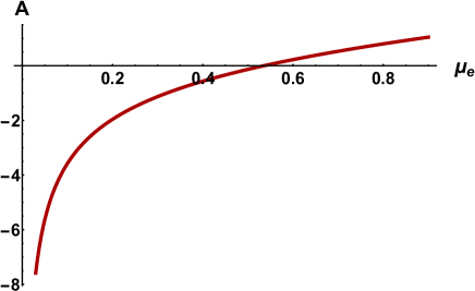
Figure 1: The variation of nonlinear coefficient $A$ with $\mu_{e}$. Other plasma parameters are $\alpha_{1}=10^{-3}$, $\alpha_{2}=0.03$, $\delta=10^{\circ}$, $\kappa=2$, and $v_{p}\equiv v_{p+}$.

Now, by taking the next higher-order terms, the equation of continuity, momentum equation, and Poisson’s equation can be written as

$$\frac{\partial n_{d}^{(1)}}{\partial\tau}-v_{p}\frac{\partial n_{d}^{(2)}}{\partial\xi}+l_{x}\frac{\partial u_{dx}^{(1)}}{\partial\xi}+l_{y}\frac{\partial u_{dy}^{(1)}}{\partial\xi}+l_{z}\frac{\partial u_{dz}^{(2)}}{\partial\xi}$$

$$\hskip 51.21504pt+l_{z}\frac{\partial}{\partial\xi}\Big{(}n_{d}^{(1)}u_{dz}^{(1)}\Big{)}=0,$$ (32)

$$\frac{\partial u_{dz}^{(1)}}{\partial\tau}-v_{p}\frac{\partial u_{dz}^{(2)}}{\partial\xi}+l_{z}u_{dz}^{(1)}\frac{\partial u_{dz}^{(1)}}{\partial\xi}-\alpha_{1}l_{z}\frac{\partial\psi^{(2)}}{\partial\xi}-\eta\frac{\partial^{2}u_{hz}^{(1)}}{\partial\xi^{2}}=0,$$ (33)

$$\frac{\partial n_{i}^{(1)}}{\partial\tau}-v_{p}\frac{\partial n_{i}^{(2)}}{\partial\xi}+l_{x}\frac{\partial u_{ix}^{(1)}}{\partial\xi}+l_{y}\frac{\partial u_{iy}^{(1)}}{\partial\xi}+l_{z}\frac{\partial u_{iz}^{(2)}}{\partial\xi}$$

$$\hskip 51.21504pt+l_{z}\frac{\partial}{\partial\xi}\Big{(}n_{i}^{(1)}u_{iz}^{(1)}\Big{)}=0,$$ (34)

$$\frac{\partial u_{iz}^{(1)}}{\partial\tau}-v_{p}\frac{\partial u_{iz}^{(2)}}{\partial\xi}+l_{z}u_{iz}^{(1)}\frac{\partial u_{iz}^{(1)}}{\partial\xi}+l_{z}\frac{\partial\psi^{(2)}}{\partial\xi}$$

$$\hskip 14.22636pt+\alpha_{2}l_{z}\Biggr{[}\frac{2}{3}\frac{\partial n_{i}^{(2)}}{\partial\xi}-\frac{1}{9}\frac{\partial n_{i}^{(1)^{2}}}{\partial\xi}\Biggr{]}-\eta\frac{\partial^{2}u_{iz}^{(1)}}{\partial\xi^{2}}=0,$$ (35)

$$n_{i}^{(2)}=(1-\mu_{e})n_{d}^{(2)}+\sigma_{1}\psi^{(2)}+\sigma_{2}\psi^{(1)^{2}}.\$$ (36)

Finally, the next higher-order terms of Eqs. (6)-(9) and (12), with the help of Eqs. (22)-(36), can provide the Burgers’ equation

$$\frac{\partial\Psi}{\partial\tau}+A\Psi\frac{\partial\Psi}{\partial\xi}=C\frac{\partial^{2}\Psi}{\partial\xi^{2}},\$$ (37)

where $\Psi=\psi^{(1)}$ is used for simplicity. The nonlinear coefficient ($A$) and dissipative coefficient ($C$) are represented, respectively, as

$$A=\frac{2\sigma_{2}s_{1}^{3}v_{p}^{4}+3\alpha_{1}^{2}s_{1}^{3}l_{z}^{4}(1-\mu_{e})-81v_{p}^{6}l_{z}^{4}-F_{1}}{2\alpha_{2}v_{p}l_{z}^{2}s_{1}^{3}(\mu_{e}-1)+F_{2}},$$ (38)

$$C=\frac{\eta}{2},\$$ (39)

where $F_{1}=6\alpha_{2}s_{1}v_{p}^{4}l_{z}^{6}$, $F_{2}=-18s_{1}l_{z}^{2}v_{p}^{5}$, and $s_{1}=3v_{p}^{2}-2\alpha_{2}l_{z}^{2}$. To obtain stationary shock wave solution of this Burgers’ equation, we consider a frame of reference that advances with shock speed $U_{0}$. The space ($\zeta$) and time ($\tau$) coordinates in such frame are expressed as $\zeta=\xi-U_{0}\tau^{\prime}$ and $\tau=\tau^{\prime}$. These allow us to write the stationary shock wave solution as [48, 49]

$$\Psi=\Psi_{m}\Big{[}1-\tanh\bigg{(}\frac{\zeta}{\Delta}\bigg{)}\Big{]},\$$ (40)

where the amplitude $\Psi_{m}$ and the width $\Delta$ is given by

$$\Psi_{m}=\frac{U_{0}}{A},~{}~{}\text{and}~{}~{}\Delta=\frac{2C}{U_{0}}.\$$ (41)

It can be seen from Eq. (33) that the amplitude of the shock wave becomes infinity corresponding to the value of $A=0$ (due to $C>0$ and $U_{0}>0$), and this refers to that our theory (specially, the RPM) is only valid for the small amplitude waves.

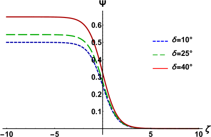
Figure 2: The variation of $\Psi$ with $\zeta$ for different values of $\delta$ under consideration of $\mu_{e}>\mu_{ec}$. Other plasma parameters are $\alpha_{1}=10^{-3}$, $\alpha_{2}=0.03$, $\eta=0.3$, $\kappa=2$, $\mu_{e}=0.8$, $U_{0}=0.2$, and $v_{p}\equiv v_{p+}$.

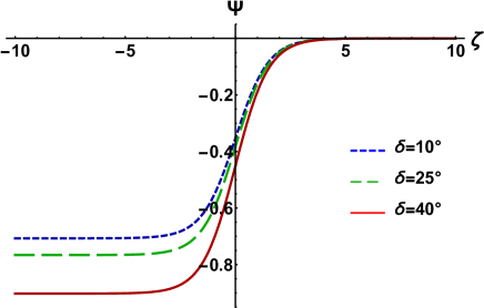
Figure 3: The variation of $\Psi$ with $\zeta$ for different values of $\delta$ under consideration of $\mu_{e}<\mu_{ec}$. Other plasma parameters are $\alpha_{1}=10^{-3}$, $\alpha_{2}=0.03$, $\eta=0.3$, $\kappa=2$, $\mu_{e}=0.4$, $U_{0}=0.2$, and $v_{p}\equiv v_{p+}$.

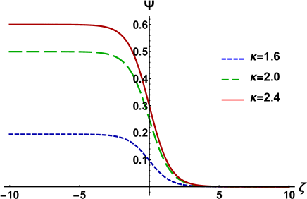
Figure 4: The variation of $\Psi$ with $\zeta$ for different values of $\kappa$ under consideration of $\mu_{e}>\mu_{ec}$. Other plasma parameters are $\alpha_{1}=10^{-3}$, $\alpha_{2}=0.03$, $\delta=10^{\circ}$, $\eta=0.3$, $\mu_{e}=0.8$, $U_{0}=0.2$, and $v_{p}\equiv v_{p+}$.

4 Numerical analysis

The balance between nonlinearity and dissipation leads to generate DIASHWs in a three-component magnetized DPM. We have numerically analyzed the variation of $A$ with $\mu_{e}$ in Fig. 1, and it is obvious from this figure that (a) $A$ can be negative, zero, and positive depending on the values of $\mu_{e}$; (b) the value of $\mu_{e}$ for which $A$ becomes zero is known as critical value of $\mu_{e}$ (i.e., $\mu_{ec}$), and the $\mu_{ec}$ for our present analysis is almost $0.55$; and (c) the parametric regimes for the formation of positive (i.e., $\psi>0$) and negative (i.e., $\psi<0$) potential shock structures can be found corresponding to $A>0$ and $A<0$.

It is clear from Figs. 2 and 3 that (a) with the increase of the oblique angle ($\delta$), the magnitude of the amplitude of the positive and negative shock structures increases, and this result agrees with the result of Hossen et al. [41]; (b) the magnitude of the negative potential is always greater than the positive potential for same plasma parameters. So, the oblique angle enhances the height of the potential shock structures.

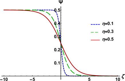
Figure 5: The variation of $\Psi$ with $\zeta$ for different values of $\eta$ under consideration of $\mu_{e}>\mu_{ec}$. Other plasma parameters are $\alpha_{1}=10^{-3}$, $\alpha_{2}=0.03$, $\delta=10^{\circ}$, $\kappa=2$, $\mu_{e}=0.8$, $U_{0}=0.2$, and $v_{p}\equiv v_{p+}$.

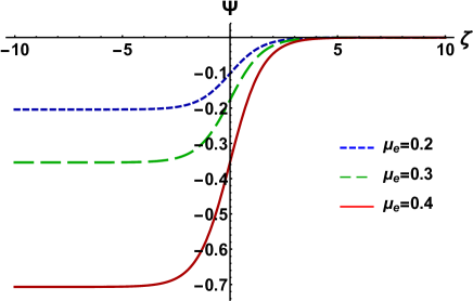
Figure 6: The variation of $\Psi$ with $\zeta$ for different values of $\mu_{e}$ under consideration of $\mu_{e}<\mu_{ec}$. Other plasma parameters are $\alpha_{1}=10^{-3}$, $\alpha_{2}=0.03$, $\delta=10^{\circ}$, $\eta=0.3$, $\kappa=2$, $U_{0}=0.2$, and $v_{p}\equiv v_{p+}$.

Figure 4 displays the variation of positive shock profile with spectral index $\kappa$, and it is evident from the figure that (a) shock height is amplified for higher values of $\kappa$, and this result agrees with the previous work of Ref. [36]; (b) positive shock height changes abruptly with the increase of the value of $\kappa$.

It is evident from Fig. 5 that there are some specific correlations between the dust-ion kinematic viscosity on the positive (under the consideration $\mu_{e}>\mu_{ec}$) shock profiles. It is really interesting that the magnitude of the amplitude of positive shock profiles is not affected by the variation of the dust-ion kinematic viscosity but the steepness of the shock profile decreases with the increase of dust-ion kinematic viscosity, and this result is in good agreement with the result of Bansal et al. [42] and Borah et al. [43].

Figure 6 illustrates the effects of the equilibrium density ratio of electrons to ions (via $\mu_{e}$) on plasma shock structures. The numerical analysis exhibits amplification in the magnitude of the amplitude of negative shock profile for higher values of $\mu_{e}$ which fully agrees with the result of Kamran et al. [44]. However, the variation of the value of $\mu_{e}$ drastically changes the height of the shock profile.

5 Conclusion

We have studied DIASHWs in a three-component magnetized DPM by considering kinematic viscosities of both negative dust and positive ion species, and inertialess super-thermal electrons. The reductive perturbation method is used to derive the Burgers’ equation. The results that have been found from our investigation can be summarized as follows:

• The parametric regimes for the formation of positive (i.e., $\psi>0$) and negative (i.e., $\psi<0$) potential shock structures can be found corresponding to $A>0$ and $A<0$.

• The magnitude of the amplitude of positive and negative shock structures increases with the oblique angle ($\delta$).

• The magnitude of the amplitude of positive and negative shock profiles is not affected by the variation of the dust-ion kinematic viscosity ($\eta$) but the steepness of the shock profile decreases with dust-ion kinematic viscosity ($\eta$).

It should be noted here that the gravitational effect is of great importance for DPM but it is beyond the scope of our present work. In future for better understanding, someone can investigate the nonlinear propagation in a three-component DPM by considering the gravitational effect. The results of our present investigation will be useful in understanding the nonlinear phenomena both in astrophysical environments such as interstellar clouds [1, 2, 3], circumstellar clouds [5, 6, 7], interplanetary space [8, 9, 10], Earth’s magnetosphere[11], Saturn’s B ring [12] and magnetosphere [13, 14], Jupiter’s magnetosphere [14, 15], cometary tails [16, 17] and in laboratory plasmas [18, 19].

References

• [1] L. Spitzer, Physical Processes in the Interstellar Medium, (Wiley, New York, 1978).
• [2] B.D. Savage and J.S. Mathis, Ann. Rev. Astron. Astrophys. 17, 73 (1979).
• [3] E. Herbst, Annu. Rev. Phys. Chem. 46, 27 (1995).
• [4] M.H. Rahman,et al., Phys. Plasmas 25, 102118 (2018); R.K. Shikha, et al., Eur. Phys. J. D 73, 177 (2019); S.K. Paul, et al., Pramana J. Phys. 94, 58 (2020); S. Jahan, et al., Commun. Theor. Phys. 71, 327 (2019); N.A. Chowdhury, et al., Phys. plasmas 24, 113701 (2017); M.H. Rahman, et al., Chin. J. Phys. 56, 2061 (2018); D.M.S. Zaman, et al., High Temp. 58, 789 (2020); S. Jahan, et al., Plasma Phys. Rep. 46, 90 (2020).
• [5] V. Ossenkopf, et al., Astron. Astrophys. 261, 567 (1992).
• [6] S.M. Andrews and J.P. Williams, Astrophys. J. 631, 1134 (2005).
• [7] C. Dijkstra, et al., Astrophy. J. 633, L133 (2005).
• [8] I.D.R. Mackinnon and F.J.M. Rietmeijer, Rev. Geophys. 25, 7 (1987).
• [9] S.A. Sandford and J.P. Bradley, Icarus 82, 146 (1989).
• [10] J.C. Liou and H.A. Zook, Icarus 124, 429 (1996).
• [11] M. Horanyi, et al., Astrophys. Space Sci. 144, 215 (1988).
• [12] T.G. Northrop and J.R. Hill, J. Geophys. Res. 88, A8 (1983).
• [13] D.H. Humes, J. Geophys. Res. 85, 5841 (1980).
• [14] T.G. Northrop and J.R. Hill, J. Geophys. Res. 88, A1 (1983).
• [15] D.H. Humes, et al., J. Geophys. Res. 79, 25 (1974).
• [16] E.P. Mazets, et al., Astron. Astrophys. 187, 699 (1987).
• [17] D.A. Gurnett, et al., Geophys. Res. Lett. 13, 3 (1986).
• [18] G.S. Selwyn, et al., J. Vac. Sci. Technol. A, 7, 2758 (1989).
• [19] L. Boufendi and A. Bouchoule, Plas. Sour. Sci. Technol. 11, A211 (2002).
• [20] T.G. Northrop and J.R. Hill, J. Geophys. Res. 87, A8 (1982).
• [21] R.L. Merlino, et al., Phys. Plasmas 5, 1607 (1998).
• [22] P.K. Shukla, Phys. Script. 45, 504 (1992).
• [23] S. Ghosh, et al., Phys. Lett. A 274, 162 (2000).
• [24] Y. Nakamura, Phys. Plas. 9, 440 (2002).
• [25] A.A. Mamun and K.S. Ashrafi, Phys. Rev. E 82, 026405 (2010).
• [26] D. Samsonov, et al., Phys. Rev. Lett. 92, 25 (2004).
• [27] M. Bacha, et al., Phys. Rev. E 85, 056413 (2012).
• [28] V.M. Vasyliunas, J. Geophys. Res. 73, 9 (1968).
• [29] A.T.Y. Lui and S.M. Krimigis, Geophys. Res. Lett. 10, 13 (1983).
• [30] D.J. Williams, et al., Geophys. Res. Lett. 15, 4 (1988).
• [31] S.P. Christon, et al., J. Geophys. Res. 93, 2562 (1988).
• [32] B.A. Shrauner and W. C. Feldman, J. Plasma Phys. 17, 123 (1977).
• [33] J.T. Gosling, et al., J. Geophys. Res. 86, 547 (1981).
• [34] N. Divine and H.B. Garrett, J. Geophys. Res. 88, 6889 (1983).
• [35] T.P. Armstrong, et al., J. Geophys. Res. 88, 8893 (1983).
• [36] A. Shah, et al., Phys. Plasmas 19, 032302 (2012).
• [37] M. Adnan, et al., Advan. Spa. Res. 53, 845 (2014).
• [38] M.M. Haider and A. Nahar, Z. Naturforsch. 72, 627 (2017).
• [39] Y.B. Zel’dovich and Y.P. Raizer, Physics of Shock Waves and High- Temperature Hydrodynamic Phenomena (Academic, New York, 1967).
• [40] B. Sahu, et al., Phys. Plasmas. 21, 103701 (2014).
• [41] M.M. Hossen, et al., High Energy Density Phys. 24, 9 (2017).
• [42] S. Bansal, et al., Eur. Phys. J. D 74, 236 (2020).
• [43] P. Borah, et al., Phys. Plasmas. 23, 103706 (2016).
• [44] M. Kamran, et al., Resul. Phys. 21, 103808 (2021) .
• [45] S.Y. El-Monier and A. Atteya, AIP Adv. 9, 045306 (2019).
• [46] M. Hassan, et al., Commun. Theor. Phys. 71, 1017 (2019); N.A. Chowdhury, et al., Plasma Phys. Rep. 45, 459 (2019); N.A. Chowdhury, et al., Contrib. Plasma Phys. 58, 870 (2018); S. Banik, et al., Eur. Phys. J. D 75, 43 (2021); N.A. Chowdhury, et al., Chaos 27, 093105 (2017); N.A. Chowdhury, et al., Vacuum 147, 31 (2018); N. Ahmed, et al., Chaos 28, 123107 (2018).
• [47] H. Washimi and T. Taniuti, Phys. Rev. Lett. 17, 996 (1966).
• [48] V.I. Karpman, Nonlinear Waves in Dispersive Media, (Pergamon Press, Oxford, 1975).
• [49] A. Hasegawa, Plasma Instabilities and Nonlinear Effects, (Springer-Verlag, Berlin, 1975).