Uncertainty relation between detection probability and energy fluctuations

Abstract

A classical random walker starting on a node of a finite graph will always reach any other node since the search is ergodic, namely it is fully exploring space, hence the arrival probability is unity. For quantum walks, destructive interference may induce effectively non-ergodic features in such search processes. We consider a tight-binding quantum walk described by a time independent Hamiltonian $H$, starting in state $|\psi_{{\rm in}}\rangle$. Under repeated projective measurements, made on a target state $|{\rm d}\rangle$, the final detection of the system is not guaranteed since destructive interference may split the Hilbert space into a bright subspace and an orthogonal dark one. Using this we find an uncertainty relation for the deviations of the detection probability $P_{{\rm det}}$ which reads

$$\Delta P\mbox{Var}(H)_{d}\geq|\langle{\rm d}|\left[H,D\right]|\psi_{{\rm in}}\rangle|^{2}.$$

Here $\Delta P=P_{{\rm det}}-|\langle\psi_{{\rm in}}|{\rm d}\rangle|^{2}$ is the deviation of the total detection probability from the initial probability of detection, $\mbox{Var}(H)_{d}$ is the variance of the energy in the detected state, and on the right hand side of the inequality we use the commutation relation of $H$ and the measurement projector $D=|{\rm d}\rangle\langle{\rm d}|$. Extensions and examples are discussed.

I Introduction

A classical random walk on a finite graph explores the system completely. In a search process a particle starts on some node of a graph and then searches for a target on another node. For classical walks on such structures the arrival probability $P_{{\rm det}}$, that is the probability that the particle starting on one node and detected eleswhere, in principle after some long time, is unity. In that sense classical random walk search on a finite graph is efficient though time wise the search can be very inefficient. The exceptions with $P_{\rm det}\neq 1$ are obvious. If the graph is decomposed into several non-connected parts, the dynamics is not ergodic, and then exploration of at least part of the space is prohibeted. Thus, the related recurrence problem becomes an issue only for an infinite system, for example a classical random walk on a lattice in dimension larger than two is non-recurrent Polya ; Redner ; Ralf .

A very different behavior is found for quantum walkers Aharonov1 ; Ambainis ; Blumen ; Salvador on finite graphs that start localized on a node of the graph. Firstly the concept of quantum arrival is not well defined, and instead we discuss the first detection, see below. Secondly, destructive interference may divide the Hilbert space into two components called dark and bright, and this yields an effect similar to classical non-ergodicity, $P_{{\rm det}}<1$. More specifically, an observer performs repeated strong measurements, made on another node, in an attempt to detect the particle Bach ; Krovi ; Krovi1 ; Varbanov ; Grunbaum ; Krapivsky ; Dhar ; Dhar1 ; Sinkovicz1 ; Harel ; Felix1 ; FelixPRA ; Lahiri ; Dubey ; Liu . In the time intervals between the measurements the dynamics is unitary. The rate of measurement attempts is $1/\tau$ where $\tau$ is a parameter of choice (see details below). Due to destructive interference, there might exist certain initial states whose amplitude vanishes at the detected node at all times and this renders them non-detectable. Such initial conditions are called dark states and they are widely encountered Caruso . In this case the mean hitting time, i.e. the mean time for detection, is infinite Krovi1 and this can be found for simple models like a quantum walk on a hyper-cube Krovi or a ring Harel . More precisely to get non-classical behavior for $P_{{\rm det}}$ the system has to have some symmetry built into it Krovi1 ; FelixLET . Generic initial states $|\psi_{{\rm in}}\rangle$ are linear combinations of dark and bright states, the latter are detected with probability one. It follows that a system starting in state $|\psi_{{\rm in}}\rangle$ has a probability to be detected that lies somewhere between zero and unity. The question remains is to quantify this probability $0\leq P_{{\rm det}}\leq 1$?

A formal solution for the detection probability was found in Krovi ; FelixLET and obtained explicitly for a few examples FelixExactKB . Since $P_{{\rm det}}$ is non-trivial if compared with the classical counterpart we will find its bound. As announced in the abstract, this is presented with an uncertainty relation, relating the detection probability, fluctuations of energy and the commutation relation of $H$ with the projection operator describing the measurement. For that aim we consider a measurement protocol with stroboscopic detection, however we argue below that the results obtained here are generic. Generally the uncertainty principle Busch describes the deviation of the quantum world from classical Newtonian mechanics. Our goal is very different. We present an approach that shows how quantum walks depart from the corresponding classical walks. Note that the uncertainty principle discussed here, an exact formal solution to the problem, and an upper bound based on symmetry were presented recently in a short communication FelixLET .

II Model and Notation

We consider quantum dynamics on a finite graph pierced by measurements. The evolution free of measurement is described by a time independent Hamiltonian $H$ and the corresponding unitary propagator. Examples include a single particle on a graph, where $H$ is a tight-binding Hamiltonian, e.g. dynamics of a particle on a ring with hops to nearest neighbours. The theory is valid in generality e.g. by identifying the graph with a Fock space, one can describe the dynamics of a many body system, see an example in Ref. Yin . Initially the particle is in state $|\psi_{{\rm in}}\rangle$ which could be a state localized on a node of the graph.

We use stroboscopic measurements at times $\tau,2\tau,...$ in an attempt to detect the particle in state $|{\rm d}\rangle$, for example on a node of the graph or an energy eigen state of $H$ etc. Specifically the measurement if successful projects the wave packet onto state $|{\rm d}\rangle$ otherwise this state is projected out and the wave function renormalised (see below). Between the measurement attempts the evolution is unitary described with $U=\exp(-iH\tau)$ and here $\hbar=1$. The outcome of a measurement is binary: either a failure in detection (no) or success (yes). Thus the string of measurements yields a sequence no, no, and in the n-th attempt a yes, though the final success is not a rule of nature. Once we detect the particle we are done, we say that $n\tau$ is the time it took to detect the particle in state $|{\rm d}\rangle$. Fixing $H$ and $\tau$ and repeating this measurement process does not mean that the particle is always detected. The question addressed here is what is the probability that the particle is detected at all, in principle after an infinite number of measurement attempts. This is the total detection probability $P_{{\rm det}}$.

This model is the quantum version of the first passage time problem Redner ; Ralf . However, here the measurements backfire and modify the dynamics. Specifically, each individual measurement is described with the collapse postulate. Namely if the system’s wave function is $|\psi\rangle$ at the moment of the detection attempt, the amplitude of finding the particle at $|{\rm d}\rangle$ is $\langle{\rm d}|\psi\rangle$. As mentioned if the particle is detected we are done. If not the amplitude on the detector is reset to zero, the wave function renormalised, and the evolution free of measurements continues until the next measurement etc. Mathematically the failed detection transforms $|\psi\rangle$, i.e. the wave function just before measurement, to $N(1-D)|\psi\rangle$ where $N$ is the normalization, and $D=|{\rm d}\rangle\langle{\rm d}|$ is the measurement projector. As mentioned in the introduction, aspects of this first detection problem, were investigated previously, in several works.

III Lower bound using the propagator

A bright state is an initial condition that is eventually detected with probability one $P_{{\rm det}}(\psi_{{\rm in}})=1$, while a dark state is never detected hence $P_{{\rm det}}(\psi_{{\rm in}})=0$. Following FelixLET ; FelixExactKB it is not difficult to show that if $|\beta\rangle$ is a normalised bright state then $U^{\dagger}|\beta\rangle$ is bright as well. We will soon present simple arguments to explain this statement but first let us point out its usefulness. Clearly it follows that $(U^{\dagger})^{k}|\beta\rangle$ is bright when $k$ is a non-negative integer. As a seed consider the following state $|\beta\rangle=U^{\dagger}|{\rm d}\rangle$. This is an obvious bright state since it is detected in the first measurement attempt with probability one, because $\langle{\rm d}|UU^{\dagger}|{\rm d}\rangle=1$. It therefore follows that the states

$$U^{\dagger}|{\rm d}\rangle,\cdots,(U^{\dagger})^{k}|{\rm d}\rangle\cdots$$ (1)

are all bright.

Why is $U^{\dagger}|\beta\rangle$ bright in the first place? As is well known, the energy basis is complete. Less well known is that we may construct a complete set of stationary eigenstates of $H$ which are either bright or dark FelixExactKB . These form a complete set which a priori is not trivial since in principle one could imagine a situation where the Hilbert space is divided into (say) dark, bright, and grey states, the latter are states that are detected with probability less than one but larger than zero. In FelixExactKB we present a formula for the stationary dark and bright states, making this statement more explicit, but for now all we need to know is that the finite Hilbert space can be divided into these two orthogonal subspaces denoted ${\cal H}_{B}$ (bright) and ${\cal H}_{D}$ (dark). Let $|E_{j}^{D}\rangle$ be a specific stationary dark state, and $j$ is an index enumerating this family of states. Then clearly $\langle E_{j}^{D}|U^{\dagger}|\beta\rangle=0$ since the dark state is orthogonal to the bright one and $\langle E_{j}^{D}|U^{\dagger}$ gives a phase $\exp(iE_{j}\tau)$ where $E_{j}$ is the corresponding energy level. It follows that $U^{\dagger}|\beta\rangle$ has no dark component in it and hence it is bright. Thus the whole approach is based on the fact that we may divide a finite Hilbert space to a dark and bright subspaces. These are related to the so called Zeno sub-spaces used to constrain dynamics to part of the Hilbert space Facchi ; Pascazio ; Gherardini . In contrast we consider generic initial conditions that belong both to the dark and the bright components of the Hilbert space and this gives non-trivial detection probability.

We notice in the same way that the sequence

$$U|\beta\rangle,\cdots U^{k}|\beta\rangle\cdots$$ (2)

is also bright. As a consequence, since $U^{\dagger}|{\rm d}\rangle$ is bright, the state $UU^{\dagger}|{\rm d}\rangle$ is also bright. So when starting at the state $|{\rm d}\rangle$ the system is detected with probability one, as was shown previously using other methods Grunbaum .

We now see that

$$|{\rm d}\rangle,U^{\dagger}|{\rm d}\rangle\cdots$$ (3)

are bright states. However they are not orthogonal. We may choose the first two terms and construct two bright orthogonal vectors

$$|\tilde{\chi}_{1}\rangle=|{\rm d}\rangle\ \mbox{and}\ |\tilde{\chi}_{2}\rangle=N\left(|{\rm d}\rangle-{U^{\dagger}|{\rm d}\rangle\over\langle{\rm d}|U^{\dagger}|{\rm d}\rangle}\right)$$ (4)

where $N$ is a normalization constant and $|{\rm d}\rangle$, the detected state, is not an eigenstate of $U^{\dagger}$. We note that using a similar approach it is not difficult to obtain further orthogonal bright states though in practice we perform this step (see below) with a computer program to avoid the algebra. Further, the infinite sequence in Eq. (3) is over-complete. To construct a bright space we must find a set of orthogonal vectors forming a basis using for example the Gram-Schmidt method. Formally the bright space is

$${\cal H}_{B}=\mbox{Span}\{|{\rm d}\rangle\ ,U|{\rm d}\rangle\ ,U^{2}|{\rm d}\rangle\ ,\cdots\}$$ (5)

where $\mbox{Span}\{...\}$ is the set containing all linear combinations of vectors of the states in the parentheses. Below we will construct this space explicitly for some simple examples, however in general this demands crunching linear algebra. For this reason the here-presented uncertainty relation, is useful in many cases.

When we have found a complete orthonormal basis vectors, which are either dark or bright states, the detection probability is given by Krovi ;

$$P_{{\rm det}}=\sum_{\tilde{\beta}\in{\cal H}_{B}}|\langle\tilde{\beta}|\psi_{{\rm in}}\rangle|^{2},$$ (6)

where the summation is over a bright basis which as usual has many representations. It follows that

$$P_{{\rm det}}\geq|\langle\tilde{\chi}_{1}|\psi_{{\rm in}}\rangle|^{2}+|\langle\tilde{\chi}_{2}|\psi_{{\rm in}}\rangle|^{2}.$$ (7)

We then find

$$P_{{\rm det}}\geq{|\langle{\rm d}|U|\psi_{{\rm in}}\rangle|^{2}\over 1-|\langle{\rm d}|U|{\rm d}\rangle|^{2}}$$ (8)

provided that the initial state and the detected one are orthogonal $\langle{\rm d}|\psi_{{\rm in}}\rangle=\langle\tilde{\chi}_{1}|\psi_{{\rm det}}\rangle=0$. Note that $U|\psi_{{\rm in}}\rangle$ and $U|{\rm d}\rangle$ are solutions of the Schrödinger equation in the absence of measurement starting with $|\psi_{{\rm in}}\rangle$ and $|{\rm d}\rangle$ respectively, hence the lower bound relates the dynamics of a measurement free process at time $\tau$ to the detection probability which is the outcome of the repeated measurement process. The bound generally depends on $\tau$ and at least in principle one may search for $\tau$ that maximizes its right hand side. When $\tau$ is small, we may expand the propagator to second order $U\sim 1-iH\tau-H^{2}\tau^{2}/2$ and then find

$$P_{{\rm det}}\geq{|\langle{\rm d}|H|\psi_{{\rm in}}\rangle|^{2}\over\mbox{Var}(H)_{{\rm d}}}$$ (9)

where

$$\mbox{Var}(H)_{{\rm d}}=\langle{\rm d}|H^{2}|{\rm d}\rangle-\langle{\rm d}|H|{\rm d}\rangle^{2}$$ (10)

characterises the fluctuation of the energy in the detected state. Thus the detection probability is bounded by the transition matrix from the initial to the detected state divided by the fluctuations of the energy in the latter. What comes to us as a surprise is that this result is valid for practically any $\tau$, as we will show after a few remarks.

Remark 1. Our results are valid for finite size systems, like finite graphs. For infinite systems, it is not always possible to divide the Hilbert space into two sub-spaces dark and bright. For example for a one-dimensional tight binding quantum walk on a lattice, with jump amplitude to nearest neighbours, starting on a node called the origin and measuring there, the non-zero detection probability is less than unity Harel . This means that $|{\rm d}\rangle$ is not bright for an infinite system, which is physically obvious as the wave packet can spread to infinity and hence the particle can escape detection. In this case $|{\rm d}\rangle$ is a grey state.

Remark 2. The states $|{\rm d}\rangle,...U^{k}|{\rm d}\rangle...$ are bright and similarly with $U^{\dagger}$. Can we find a bright state $|\beta^{\prime}\rangle$ orthogonal to these states? The answer is negative, and hence these states can be used to span the bright subspace. Assume $|\beta^{\prime}\rangle$ is an initial condition $|\psi_{{\rm in}}\rangle$ which is bright. At first measurement at time $\tau$ the amplitude of detection is $\langle{\rm d}|U|\beta^{\prime}\rangle$ however this is zero by the assumption that $|\beta^{\prime}\rangle$ is orthogonal to the just obtained set of bright states. We may continue with this reasoning for the second, third, etc measurements, and we see that amplitude of detection of $|\beta^{\prime}\rangle$ is always zero. It follows that state $|\beta^{\prime}\rangle$ is not bright.

IV Uncertainty relation

Let $|\beta\rangle$ be a bright state, then also $f(H)|\beta\rangle$ is bright where $f(.)$ is an analytical function. Indeed similar to the previous section $\langle E_{j}^{D}|f(H)|\beta\rangle=0$ and hence the state $f(H)|\beta\rangle$ has no dark element, meaning it is bright. As we showed already the state $|{\rm d}\rangle$ is bright so we find a sequence of bright states

$$|{\rm d}\rangle,H|{\rm d}\rangle,\cdots,H^{k}|{\rm d}\rangle\cdots.$$ (11)

We use the same approach as in the previous section, namely we use the first two states and find two orthonormal bright states

$$|\chi_{1}\rangle=|{\rm d}\rangle\ \mbox{and}\ |\chi_{2}\rangle=N\left(|{\rm d}\rangle-{H|{\rm d}\rangle\over\langle{\rm d}|H|{\rm d}\rangle}\right).$$ (12)

The normalization constant is given by $|N|^{2}=(\langle H\rangle_{\rm d})^{2}/\mbox{Var}(H)_{\rm d}$ where $\langle H\rangle_{\rm d}=\langle{\rm d}|H|{\rm d}\rangle$. Since $H$ is Hermitian, inserting Eq. (12) in Eq. (7), and assuming no overlap of the initial state with the detection one, $\langle{\rm d}|\psi_{{\rm in}}\rangle=0$ we get Eq. (9). Thus that formula is valid for any $\tau$.

For the more general case when the initial overlap with the detection state is not zero, we define

$$\Delta P=P_{{\rm det}}-|\langle{\rm d}|\psi_{{\rm in}}\rangle|^{2}.$$ (13)

Since $|\langle{\rm d}|\psi_{{\rm in}}\rangle|^{2}$ is the square of the overlap of the initial state and the detected one, it gives the probability to detect the particle in a single-shot measurement at time $t=0$. So $\Delta P$ is the difference between the probability of detection after repeated measurements and the initial probability of detection. Using Eqs. (7,12) and $\langle{\rm d}|H(D-1)|\psi_{{\rm in}}\rangle=\langle{\rm d}|\left[H,D\right]|\psi_{{\rm in}}\rangle$ we find

$$\Delta P\mbox{ Var}(H)_{{\rm d}}\geq|\langle{\rm d}|\left[H,D\right]|\psi_{{\rm in}}\rangle|^{2}.$$ (14)

Here $\left[H,D\right]$ is the commutator of the Hamiltonian and the projector describing the measurement. If $|\psi_{{\rm in}}\rangle=|{\rm d}\rangle$ the right hand side is equal zero and we find $P_{{\rm det}}\geq 1$, hence here the uncertainty relation indicates that the detection probability is unity.

Remark 3. The matrix element $\langle{\rm d}|H|{\rm d}\rangle$ can always be set to be non-zero by a global shift of the energy, hence $|{\rm\chi}_{2}\rangle$ is well defined. In the final result we can switch back to any choice of energy scale, since the $\mbox{Var}(H)_{d}$ is insensitive to the definition of the zero of energy.

Remark 4. For the stroboscopic sampling, recurrences and revivals imply that special sampling times $\tau$ defined through $\Delta E\tau=2\pi k$ exhibit resonances Grunbaum ; Harel such that the bounds based on energy are invalid. Here $\Delta E$ is the energy difference between any pair of energy levels in the system. In this case the starting point of the analysis should be Eq. (1) and not Eq. (11).

Remark 5. We believe that our results are generally valid for other detection protocols, for examples when we sample the system randomly in time following a Poissonian process Varbanov . This is because the dark and bright spaces are not sensitive to the timing of the measurements. Exceptional $\tau$’s mentioned in the previous remark are clearly not something to worry about in this more general case.

V The reverse dark approach

Assume $|\delta\rangle$ is a normalised dark state, then as before the states $U^{k}|\delta\rangle,H^{k}|\delta\rangle,f(H)|\delta\rangle$ are dark as well. In fact since by definition a system initially in a dark state $|\psi_{{\rm in}}\rangle=|\delta\rangle$ is never detected, it follows immediately that $U^{k}|\delta\rangle$ and $H^{k}|\delta\rangle$ are dark (see remark below). However, there is no symmetry between dark and bright states, in the sense that, every system has at least one bright state $|{\rm d}\rangle$, but not every system necessarily has a dark state. As we show in FelixExactKB totally bright systems have non-degenerate energy levels and all the energy eigenstates having a finite overlap with the detected state. Still let us assume that we find a state $|\delta\rangle$, which is dark, we can then apply nearly the same strategy as before to find an upper bound for $P_{{\rm det}}$. We use $|\delta\rangle$ and $H|\delta\rangle$ to construct two orthonormal dark states

$$|\xi_{1}\rangle=|\delta\rangle,\ \ |\xi_{2}\rangle=N\left(|\delta\rangle-{H|\delta\rangle\over\langle\delta|H|\delta\rangle}\right),$$ (15)

where $N$ is a normalization constant. Clearly here we assume that the dark state $|\delta\rangle$ is not a stationary state of the system, since otherwise $|\xi_{2}\rangle$ is not defined. Analogous to Eq. (6) the detection probability is FelixExactKB

$$P_{{\rm det}}=1-\sum_{\tilde{\delta}\in{\cal H}_{D}}|\langle\tilde{\delta}|\psi_{{\rm in}}\rangle|^{2}.$$ (16)

Here the summation is over a basis of the subspace ${\cal H}_{D}$. Since all the terms in the sum are clearly non-negative

$$P_{{\rm det}}\leq 1-|\langle\xi_{1}|\psi_{{\rm in}}\rangle|^{2}-|\langle\xi_{2}|\psi_{{\rm in}}\rangle|^{2}.$$

For simplicity assume that $\langle\delta|\psi_{{\rm in}}\rangle=0$ then using the normalization $N$ we find

$$P_{{\rm det}}\leq 1-{|\langle\delta|H|\psi_{{\rm in}}\rangle|^{2}\over\mbox{Var}(H)_{\delta}}.$$ (17)

Now we have an upper bound. As mentioned in the introduction, the detection probability even for small quantum systems on a graph, can be less than unity, unlike the corresponding classical walks. So this is a useful bound provided that we can identify $|\delta\rangle$. Notice that the variance of energy is now obtained with respect to the dark state $|\delta\rangle$. Of course this state is dark with respect to a state $|{\rm d}\rangle$ so while the detector does not appear explicitly in our formula, it is obviously important.

We now relax the condition $\langle\delta|\psi_{{\rm in}}\rangle=0$. Let $P_{{\small ND}}=1-|\langle\delta|\psi_{{\rm in}}\rangle|^{2}$ be the probability that initially the system is not in the dark state $|\delta\rangle$ (hence the subscript ${\small ND}$). We consider the deviation $\delta P=P_{ND}-P_{{\rm det}}$, and find

$$\delta P\mbox{Var}(H)_{\delta}\geq|\langle\delta|\left[H,|\delta\rangle\langle\delta|\right]|\psi_{{\rm in}}\rangle|^{2}.$$ (18)

Unlike the lower bound Eq. (14), here the commutator on the right hand side, is between the Hamiltonian and a projector of the dark state while previously the commutator was of $H$ and the operator describing the measurement.

VI Further improvement of the uncertainty relation

When $\langle{\rm d}|[H,D|\psi_{{\rm in}}\rangle=0$ the uncertainty relation Eq. (14) does not provide useful information on $\Delta P$. Such situations can be found for quantum walks on a graph and we encounter them frequently in the example section. This effect is easy to understand. Assume that initially the particle is localised on a node of a graph while it is detected on a another distant node, in particular $\langle{\rm d}|\psi_{{\rm in}}\rangle=0$. Then if the hopping amplitudes are short ranged, the matrix element of $H$ between the two distant nodes is zero and then the lower bound is not useful.

For such cases we consider two other orthonormal bright states

$$|\chi_{1}\rangle=|{\rm d}\rangle\ \mbox{and}\ |\chi_{2}\rangle=N\left(|{\rm d}\rangle-{H^{s}|{\rm d}\rangle\over\langle{\rm d}|H^{s}|{\rm d}\rangle}\right)$$

where $s$ is a positive integer and when $s=1$ we get the previously examined case. The normalization is $|N|^{2}=(\langle H^{s}\rangle_{d})^{2}/\mbox{Var}(H^{s})_{d}$ where as before $\langle H^{s}\rangle_{d}=\langle{\rm d}|H^{s}|{\rm d}\rangle$ and $\mbox{Var}(H^{s})\rangle_{d}=\langle{\rm d}|H^{2s}|{\rm d}\rangle-\langle{\rm d}|H^{s}|{\rm d}\rangle^{2}$. Using Eq. (7) we find

$$\Delta P\mbox{Var}(H^{s})_{d}\geq|\langle{\rm d}|\left[H^{s},D\right]|\psi_{{\rm in}}\rangle|^{2}.$$ (19)

This relation between $\Delta P$, and the commutator of $H^{s}$ and the projector $D$ is clearly $s$ dependent. We will follow two approaches. In the first we choose the smallest $s$ such that the right hand side of the uncertainty relation is not equal zero. The second is to choose $s$ in such a way to maximize the lower bound of $P_{{\rm det}}$. In the first approach and if $H$ is described by an adjacency matrix, $s$ has a simple physical meaning as it is the distance between the assumed localised initial state and the detector state, see further details below. The first approach is the quickest way to gain insight, while the second can be used to systematically improve the result.

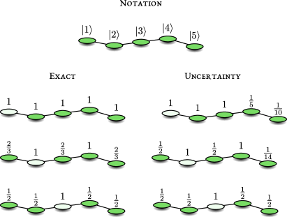
Figure 1: A quantum walk on a line with five sites. The initial condition is any localised state denoted with circles with an interior coloured green. The detected state $|{\rm d}\rangle$ is the circle with a white interior. Here we present the notation used in the text, the exact results of $P_{{\rm det}}$ and the lower bound found using the uncertainty relation. For example starting on $|1\rangle$ and measuring on $|2\rangle$ we have $P_{{\rm det}}=2/3$ while the uncertainty relation gives $P_{{\rm det}}\geq 1/2$.

VII Quantum walks on graphs

We consider a quantum walk of a single particle on a graph modelled with a tight-binding Hamiltonian. In our examples $H$ is described by an adjacency matrix. Thus the particle can occupy nodes of a graph, the edges/connections describe hopping amplitudes. All these amplitudes are identical and on site energies are set to zero. In the schematic figures of graphs under investigation, the circle with the light interior on a vertex describes the measured state $|{\rm d}\rangle$, e.g. Fig. 1. We will focus on initial conditions localised on another node (full circle) and also on the initial condition spread uniformly on the graph. Our goal is to find exact expressions for $P_{\rm det}$ using simple examples and compare the latter to the uncertainty relation.

VII.1 Finite line

We consider a quantum walk on a finite line with $L$ nodes, focusing on the example of $L=5$. The localised basis is $|r\rangle$ with $r=1,\cdots L$, so one may think of the end points as reflecting boundaries. This will soon be compared with a ring which has periodic boundaries. The Hamiltonian reads:

$$H=\gamma\left(\begin{array}[]{ c c c c c}0&1&0&0&0\\ 1&0&1&0&0\\ 0&1&0&1&0\\ 0&0&1&0&1\\ 0&0&0&1&0\end{array}\right).$$ (20)

The hopping energy $\gamma$ is set to unity hereafter. Below we modify the location of the detector, and see its effect on the detection probability and the uncertainty principle. For schematics and summary of the results see Fig. 1.

The transition to $|{\rm d}\rangle=|1\rangle$. Measurement is made on the left most node $|{\rm d}\rangle=|1\rangle$ which from symmetry is the same as the choice $|{\rm d}\rangle=|5\rangle$. We use $|{\rm d}\rangle,H|{\rm d}\rangle\cdots$ to construct the bright subspace and besides obvious normalization we get

$${\cal H}_{B}=\mbox{Span}\left\{|1\rangle,|2\rangle,|1\rangle+|3\rangle,2|2\rangle+|4\rangle,2|1\rangle+3|3\rangle+|5\rangle\right\}.$$

Since the dimension of the Hilbert space is five and since the above states are linearly independent, we have no dark subspace. Hence we are done: the detection probability of any initial condition $|\psi_{{\rm in}}\rangle$ is unity.

Aside. For a quantum walk on a finite line, i.e. a lattice stretching from $|1\rangle$ to $|L\rangle$, with a time independent $H$, and hops to nearest neighbours only (not necessarily translation invariant as in our example), any initial state $|\psi_{{\rm in}}\rangle$ is detected with probability one if the measurement is performed on the end points $|1\rangle$ or $|L\rangle$. This conclusion is immediate since the action of $H^{k}$ on the detected state $|1\rangle$ gives $L$ linearly independent vectors, which is the dimension of the Hilbert space.

Let us check the uncertainty principle starting with $|\psi_{{\rm in}}\rangle=|2\rangle$. We have $\mbox{Var}(H)_{1}=\langle 1|H^{2}|2\rangle-\langle 1|H|1\rangle^{2}=1$ and the transition amplitude $\langle 2|H|1\rangle=1$ hence

$$P_{{\rm det}}(2\to 1)\geq{|\langle 2|H|1\rangle|^{2}\over\mbox{Var}(H)_{1}}=1.$$ (21)

So here the uncertainty principle gives the exact result, since clearly $P_{{\rm det}}(2\to 1)\leq 1$.

For the other starting points in the system, namely the transitions $|r\rangle\to|1\rangle$ we use $s=r-1$ namely $s$ is equal to the distance between the initial state and detected one. Our results are summarized in Fig. 1 and read: $P_{{\rm det}}(2\to 1)\geq 1,P_{{\rm det}}(3\to 1)\geq 1,P_{{\rm det}}(4\to 1)\geq 1/5,P_{{\rm det}}(5\to 1)\geq 1/10$. We see that more distant initial states depart from the exact result $P_{{\rm det}}=1$. If $|\psi_{{\rm in}}\rangle=|{\rm d}\rangle$ we mentioned already that the uncertainty relation with $s=0$ gives $P_{{\rm det}}\geq 1$. This means that the particle is detected with probability one $P_{{\rm det}}(1\to 1)=1$.

So far we had no overlap between initial and detected states. For the uniform initial state $|\psi_{{\rm in}}\rangle=\sum_{r=1}^{5}|r\rangle/\sqrt{5}$ we find $P_{{\rm det}}\geq 6/25$ where we used $s=1$ (as mentioned the exact detection probability is unity). We will later optimise the choice of $s$ to see how one may improve the prediction of the uncertainty relation.

Detector on $|{\rm d}\rangle=|2\rangle$. The bright subspace is spanned by $|{\rm d}\rangle,H|{\rm d}\rangle,\cdots H^{3}|{\rm d}\rangle$ namely

$${\cal H}_{B}=\mbox{Span}\left\{|2\rangle\ ,|1\rangle+|3\rangle\ ,2|2\rangle+|4\rangle\ ,2|1\rangle+3|3\rangle+|5\rangle\right\}.$$

Here $H^{4}|{\rm d}\rangle$ is also bright but is easily shown to be a linear combination of $|{\rm d}\rangle$ and $H^{2}|{\rm d}\rangle$. From these states it is easy construct an orthonormal bright basis

$$\left\{|2\rangle\ ,(|1\rangle+|3\rangle)/\sqrt{2}\ ,|4\rangle\ ,(2|5\rangle+|3\rangle-|1\rangle)/\sqrt{6}\right\}.$$ (22)

Hence the dimension of the bright subspace is four, and the dark subspace has one state in it. This vector is orthogonal to the bright basis Eq, (22) and hence it is easy to see that it is given by

$$|\delta\rangle={|1\rangle-|3\rangle+|5\rangle\over\sqrt{3}}.$$ (23)

We have $H|\delta\rangle=0$; hence this state is a stationary state with an eigenvalue equal to zero. It is easy to see why this is a dark state: its amplitude on the detector is zero for any time. Using Eq. (16) $P_{{\rm det}}=1-|\langle\delta|\psi_{{\rm in}}\rangle|^{2}$ we get the exact values of $P_{{\rm det}}(1\to 2)=P_{{\rm det}}(3\to 2)=P_{{\rm det}}(5\to 2)=2/3$ and $P_{{\rm det}}(4\to 2)=P_{{\rm det}}(2\to 2)=1$. Compared with the case when the detector was on the edge we get values for $P_{{\rm det}}$ which depart from the classical case of unit detection probability. In Fig. 1. we compare these results with the uncertainty principle: $P_{{\rm det}}(1\to 2)\geq 1/2,P_{{\rm det}}(3\to 2)\geq 1/2,P_{{\rm det}}(4\to 2)\geq 1,P_{{\rm det}}(4\to 2)\geq 1/14$, where again we took $s$ to be the distance between initial and detected state. For the uniform initial state we get $P_{{\rm det}}=14/15$ while the uncertainty principle gives $P_{{\rm det}}\geq 13/25$ when we choose $s=1$.

It is easy to extend these results for a segment of length $L=2k+1$, and $k=1,2,\cdots$. We measure on $|2\rangle$ or $|L-1\rangle$ and then we have one and only one dark state. This state is an eigenstate $|\delta\rangle=(1,0,-1,0,1,0,-1,\cdots)/\sqrt{k+1}$ hence

$$P_{{\rm det}}(r\to 2)=\left\{\begin{array}[]{ c c }{k\over k+1}&\ \mbox{if r is odd}\\ 1&\ \mbox{ r is even}\end{array}\right.$$ (24)

On the other hand if $L$ is even we have no dark subspace. The detection probability is unity. Thus depending wether $L$ is even or odd we may get a dark subspace or a completely bright situation.

Detector on $|{\rm d}\rangle=|3\rangle$. We now consider the detection on the middle point $|3\rangle$ as this yields further symmetry in the problem. The states $|{\rm d}\rangle,H|{\rm d}\rangle$ and $H^{2}|{\rm d}\rangle$ are bright and are easy to evaluate $\left\{|3\rangle\ ,|2\rangle+|4\rangle\ ,|1\rangle+2|3\rangle+|5\rangle\right\}.$ It is then easy to construct the dark space, as we have only two dark states orthogonal to these bright states a dark basis is $\left\{|\delta_{1}\rangle,|\delta_{2}\rangle\right\}$ with $|\delta_{1}\rangle=(|2\rangle-|4\rangle)/\sqrt{2}$ and $|\delta_{2}\rangle=(|1\rangle-|5\rangle)/\sqrt{2}$. It is easy to understand why these states are dark as they interfere destructively on the detector on $|3\rangle$ in such a way that the amplitude of detecting the particle there is zero. We also have $H|\delta_{1}\rangle=|\delta_{2}\rangle$ and $H|\delta_{2}\rangle=|\delta_{1}\rangle$. Using the dark states and Eq. (16) we find that $P_{{\rm det}}(r\to 3)=1/2$ for any initial state $|r\rangle$ the exception is the return problem $|3\rangle\to|3\rangle$ which is detected with probability one.

Considering the transition $|2\rangle\to|3\rangle$ we may use the two uncertainty relation, one with the detector state and the second with the dark state $|\delta_{2}\rangle$ to get:

$${1\over 2}\leq P_{{\rm det}}(2\to 3)\leq{1\over 2}.$$ (25)

So here the uncertainty relations give the exact result. The same holds for the transition $1\to 3$ and the other transitions are clearly identical from symmetry. The results are summarized in Fig. 1.

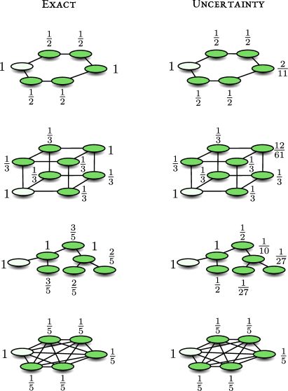
Figure 2: For a quantum walk starting on a node of the graph and measured elsewhere we present the exact result for the detection probability which depend’s on the location of the starting point. Also shown is the lower bound obtained with the uncertainty principle. We choose $s$ as the smallest integer for which the uncertainty principle is non trivial, namely the case where $\langle\psi_{{\rm in}}|H^{s}|{\rm d}\rangle\neq 0$, this is the distance between the measured site and the initial condition.

VII.2 Enumeration of paths approach

Let $H=\gamma A$ where $A$ is the adjacency matrix of some graph. We set the energy scale $\gamma=1$ as it does not control the detection probability (like the sampling rate $1/\tau$). Thus for the Hamiltonian under investigation, all bonds in the system are identical and on-site energies are zero. So $H_{ii}=0$ while $H_{{ij}}=1$ if the states are connected, zero otherwise. An example is the segment of size five just considered. As mentioned, the detection probability for the return problem $|{\rm d}\rangle\to|{\rm d}\rangle$ is unity, hence below we consider only the transition problem from some localised initial state $|r\rangle$ to another orthogonal localised state $|{\rm d}\rangle$. In this case we can use a path counting approach to find a useful bound for $P_{{\rm det}}$.

We have

$$H^{s}|{\rm d}\rangle=\sum_{\mbox{s paths}}|j\rangle$$ (26)

where the sum is over all states $|j\rangle$ which are end points of paths starting on $|{\rm d}\rangle$ and whose length is $s$. Clearly

$${\cal N}_{r\to d}(s)=\langle r|H^{s}|{\rm d}\rangle$$ (27)

is the number of paths starting on $|r\rangle$ and ending at $|{\rm d}\rangle$ whose length is $s$. We then find from the uncertainty relation

$$P_{{\rm det}}(r\to{\rm d})\geq{\left[{\cal N}_{r\to{\rm d}}(s)\right]^{2}\over{\cal N}_{{\rm d}\to{\rm d}}(2s)-\left[{\cal N}_{{\rm d}\to{\rm d}}(s)\right]^{2}}$$ (28)

the denominator is the variance of $H^{s}$ in the detector state. For example when $|r\rangle$ is the nearest neighbour of $|{\rm d}\rangle$ we choose $s=1$ and get

$$P_{{\rm det}}\left(r\to{\rm d}\right)\geq{1\over\#n.n}$$ (29)

where in the denominator we have the number of nearest neighbours. This is the reason why for the example of the line we got for nearest neighbours $P_{{\rm det}}\geq 1/2$ while for the two edge states, which have only one nearest neighbour, we got $P_{{\rm det}}\geq 1$. The bound depends on $s$ and this can be used to our advantage. What is clear is that we must choose $s$ to be larger or equal to the distance between the starting point to the measured one, otherwise the numerator in Eq. (28) is equal zero.

VII.3 The benzene like ring

We now consider the tight-binding Hamiltonian for a particle on a ring with six sites Harel

$$H=\gamma\sum_{i=0}^{5}[|i\rangle\langle i+1|+|i\rangle\langle i-1|]$$ (30)

see top left panel in Fig. 2 for schematics. Here we use periodic boundary conditions hence $|6\rangle=|0\rangle$. Similar to the previous example the energy scale $\gamma$ is irrelevant for the determination of $P_{{\rm det}}$ hence we may set $\gamma=1$ and then $H$ is the adjacency matrix of the benzene like ring. To see that $\gamma$ is irrelevant note that both the left hand side and the right hand side of the uncertainty relation Eq. (14) scale proportional to $\gamma$ hence it can be canceled out. This holds also from the exact solution to the problem Harel and is not limited to the example under study FelixLET . The repeated measurements are made on a site we call $|{\rm d}\rangle=|0\rangle$ while from symmetry all sites are identical.

With the method of enumeration of paths we consider three transitions $1\to 0$, $2\to 0$ and $3\to 0$. Since the detector on the ring has two nearest neighbours, $P_{{\rm det}}(1\to 0)\geq 1/2$. For the transition $2\to 0$ and $3\to 0$ we will use $s=2$ and $s=3$ respectively. Notice that we have only one path of length two for the transition $2\to 0$ while for the transition $3\to 0$ we have two paths of length three. Elementary path counting gives ${\cal N}_{0\to 0}(4)-[{\cal N}_{0\to 0}(2)]^{2}=2$ for $s=2$ while ${\cal N}_{0\to 0}(6)-[{\cal N}_{0\to 0}(3)]^{2}=22$ for $s=3$, hence we get $P_{{\rm det}}(2\to 0)\geq 1/2$ and $P_{{\rm det}}(3\to 0)\geq 2/11$. These results are summarized in the upper right panel of Fig. 2. We now analyse the problem exactly.

In Eq. (11) we showed that $|\psi_{{\rm in}}\rangle$ is proportional to any of the states $|0\rangle$, $H|0\rangle$, $H^{2}|0\rangle$ and $H^{3}|0\rangle$ then it is bright. Also $H^{4}|0\rangle$ is bright, however to construct a basis for the bright subspace ${\cal H}_{B}$ we need only the just mentioned states. Using $|{\rm d}\rangle=|0\rangle$ the bright subspace is given by

$${\cal H}_{B}=\mbox{Span}\left\{|0\rangle,{|1\rangle+|5\rangle\over\sqrt{2}},{2|0\rangle+|2\rangle+|4\rangle\over\sqrt{6}},{3|1\rangle+2|3\rangle+3|5\rangle\over\sqrt{22}}\right\}.$$

These states are nearly intuitively bright, for example the second $(|1\rangle+|5\rangle)/\sqrt{2}$ is interfering constructively on the detector situated on $|0\rangle$. On the other hand the state $(|1\rangle-|5\rangle)/\sqrt{2}$ is dark since from symmetry. The free evolution of this state gives zero amplitude on the detector. Acting with $H$ on this state and normalising we see that $(|2\rangle-|4\rangle)/\sqrt{2}$ is also dark which is again obvious from symmetry.

With this information we can solve the problem exactly. For example, consider a particle starting on

$$|1\rangle={1\over\sqrt{2}}\left(\underbrace{{|1\rangle+|5\rangle\over\sqrt{2}}}_{\mbox{bright}}+\underbrace{{|1\rangle-|5\rangle\over\sqrt{2}}}_{\mbox{dark}}\right).$$ (31)

As mentioned the first term is bright and the second dark, hence $P_{{\rm det}}(1\rightarrow 0)=1/2$. Similarly $P_{{\rm det}}(2\rightarrow 0)=1/2$ and $P_{{\rm det}}(3\rightarrow 0)=1$. The transition $5\rightarrow 0$ is identical to $1\rightarrow 0$ and similarly for $4\rightarrow 0$. Let us now see how the lower and upper bounds work.

The $1\rightarrow 0$ transition. As mentioned $|{\rm d}\rangle=|0\rangle$ and using Eq. (30) with $L-6$ $\mbox{Var}(H)_{0}=2$. For the initial condition $|\psi_{{\rm in}}\rangle=|1\rangle$ we have zero initial overlap with the detector. We find

$${1\over 2}={|\langle 0|H|1\rangle|^{2}\over\mbox{Var}(H)_{0}}\leq P_{{\rm det}}\leq 1-{|\langle\delta|H|1\rangle|^{2}\over\mbox{Var}(H)_{\delta}}={1\over 2}$$ (32)

where we used as a dark state $|\delta\rangle=(|2\rangle-|4\rangle)/\sqrt{2}$ and $\mbox{Var}(H)_{\delta}=1$. In this case the lower and upper bound coincide giving the exact result $P_{{\rm det}}=1/2$.

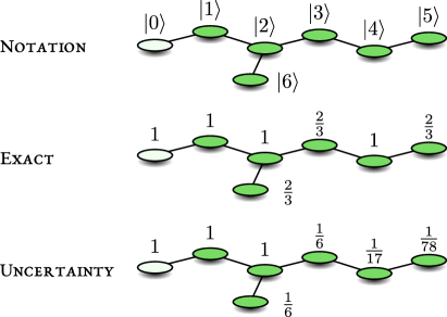
Figure 3: A system with a dangling bond where the edge state $|0\rangle$ is repeatedly measured. Note that in the absence of the bond, i.e. when node $|6\rangle$ is removed, the detection probability is unity, no matter what is the starting point. To obtain the lower bound using uncertainty we choose $s$ to be the shortest distance between the initial condition and the detected state. In Fig. 4 we improve the bound for the transition $|5\rangle\to|0\rangle$, which here gives $P_{{\rm det}}\geq 1/78$.

The $2\rightarrow 0$ transition. Since the matrix element $\langle 0|H|2\rangle=0$ we now use Eq. (19) with $s=2$ since the distance between the initial state and measured one is $2$. We find

$${1\over 2}={|\langle 2|H^{2}|0\rangle|^{2}\over\mbox{Var}(H^{2})_{0}}\leq P_{{\rm det}}\leq 1-{\langle\delta|H|2\rangle|^{2}\over\mbox{Var}(H)_{\delta}}={1\over 2}.$$ (33)

$\mbox{Var}(H^{2})_{0}=2,\mbox{Var}(H)_{\delta}=1$ and $|\delta\rangle=(|1\rangle-|5\rangle)/\sqrt{2}$. Again the lower and upper bound coincide giving the exact result.

The $3\rightarrow 0$ transition. We now set $s=3$ finding $\mbox{Var}(H^{3})_{0}=22$, while $|\langle 0|H^{3}|3\rangle|^{2}=4$ and this gives the mentioned already lower bound $2/11\leq P_{{\rm det}}\leq 1$ which is to compare with the exact result $P_{{\rm det}}=1$.

In general one could imagine several ways of how to improve the lower bound. The obvious one is to go beyond the calculation of the bright states $|{\rm d}\rangle$ and $H^{s}|{\rm d}\rangle$, namely consider a third bright state, but that means more algebra. Another option is to choose $H^{s_{1}}|{\rm d}\rangle$ and $H^{s_{2}}|{\rm d}\rangle$ as the starting point (we took $s_{1}=0$ and $s_{2}=1,2,3$). In the next section we will improve the lower bound using a simple example. However we leave the optimisation strategy of the lower bound for future work, as clearly the examples we tackle here are pedagogical. The upper bound can be tackled with symmetry arguments, which provide a different perspective FelixLET .

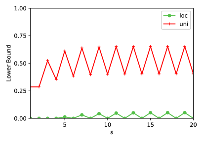
Figure 4: We demonstrate the optimisation of the uncertainty principle for a system with a dangling bond. The Fig. shows the lower bound for $P_{{\rm det}}$ versus $s$. The measurement is on node $|0\rangle$ and we consider two initial conditions: one localised $|\psi_{{\rm in}}\rangle=|5\rangle$ and the other uniform. See upper part of Fig. 3 for schematics and notation. Starting on node $|5\rangle$ and when $s\leq 4$ the bound is equal zero since if the initial and detected states are localised, $s$ must be larger than the distance between these states to make the approach useful. Increasing $s$ clearly leads to an improvements of the bound. The exact results are $P_{{\rm det}}=20/21$ for the uniform initial condition, and $P_{{\rm det}}=2/3$ for the initially localised state.

VII.4 Optimisations of the lower bound

Here we use a simple model of a system with a dangling bond, and consider the optimisation of the lower bound, i.e. we will soon search for the best choice of $s$. For the quantum walk on the line, when the measurement is made on the end point, we showed that the detection probability is unity. We add a perturbation to the system: one link perpendicular to the line. We will treat the example of a system with $6$ nodes on the backbone and one dangling bond, see schematics Fig. 3. Adding one dangling bond breaks the symmetry but only partially in the sense that we still find that the detection probability is not generically unity. We note that strongly disordered systems with no symmetry exhibit a classical behaviour namely $P_{{\rm det}}=1$ FelixLET .

The notation used, the exact results, and the uncertainty principle are presented here in Fig. 3 where the transition from a localised initial state to the detector on $|0\rangle$ is considered. Here $s$ is the distance between the initial condition and the detected state. Now we turn to a simple optimisation of the bound both for a localised initial state and for a uniform initial condition.

Consider the initial condition which is uniform $|\psi_{{\rm in}}\rangle=\sum_{r=0}^{6}|r\rangle/\sqrt{7}$. In this example we have only one dark state $|\delta\rangle=(|6\rangle-|3\rangle+|5\rangle)/\sqrt{3}$, and with this we find the detection probability $P_{{\rm det}}=20/21$. The uncertainty principle, with $s=1$ reads:

$$P_{{\rm det}}-{1\over 7}\geq{|\langle 0|H\left(1-|0\rangle\langle 0|\right)|\psi_{{\rm in}}\rangle|^{2}\over\mbox{Var}(H)_{0}}={1\over 7}.$$ (34)

Here $1/7$ on the left hand side is the initial overlap, and we used the detected node $|{\rm d}\rangle=|0\rangle$. This gives $P_{{\rm det}}\geq 2/7$. To improve this bound we made similar calculations with $s=2,...5$ the results are presented in Table $1$. The best lower bound is found for $s=5$, $P_{{\rm det}}\geq 167/253\simeq 0.6117$. To further improve the bound we depart from the § pen and paper approach instead using a simple program. The results for both the uniform initial condition and a localised initial state are presented in Fig. 4. This figure shows that increasing $s$ yields a better result for the lower bound, but eventually the calculation saturates while exhibiting odd/ even oscillation, Note that generally the lower bound calculations involve only the multiplication of matrices, while obtaining an orthonormal basis for the dark ${\cal H}_{D}$ or bright ${\cal H}_{B}$ subspaces, needed for the calculation of the exact expression for $P_{{\rm det}}$ Eqs. (6, 16), demands considerably more work.

$s$	1	2	3	4	5
$P_{{\rm det}}\geq$	${2\over 7}$	${2\over 7}$	${11\over 21}$	${42\over 119}$	${167\over 253}$

Table 1: For the system with a dangling bond, the detection being on $|0\rangle$, the Table gives the lower bound for the uniform initial condition versus $s$. Increasing $s$ in this range is improving the bound.

VII.5 Other examples

For not too large systems, it is relatively easy to write a simple program generating the bright states $|{\rm d}\rangle,H|{\rm d}\rangle\cdots$ and then to perform the Gram-Schmidt procedure. This way we find an orthonormal basis for the bright space ${\cal H}_{B}$. And then we can find the detection probability using Eq. (6). In Fig. 2 we present some graphs and the corresponding detection probability. Here as before the starting point is a node of a graph, and the empty circle is the position of the detector. It is striking, that when the detector is placed on a symmetry centre of the graph, $P_{{\rm det}}$ may exhibit a deficit from the classical limit of unity. Since the classical detection probability on similar graphs is unity, the deviations are of interest. So as a rule of thumb we use systems with symmetry to find deviations from classical expectations, however the symmetry may not be always obvious, so it will be the subject of our next paper.

All the examples presented here are based on rather simple graphs. This allowed us to obtain exact solutions rather easily and then estimate the performance of the uncertainty principle. For large and generally complex systems the bound can perform rather poorly. To tackle the problem one therefore needs a set of tools, and one cannot rely only on the method presented here. We mention briefly a few cases. If the system is disordered such that the energy spectrum is non-degenerate, and each stationary state has some finite overlap with the detected state, the detection probability is unity. In this case the system behaves classically and there is no need at all for a lower bound. For systems with symmetry, and hence a degenerate spectrum, an upper bound based on symmetry was found. This relates the number of equivalent states in the system $\nu$, i.e. states that are equivalent to the initial state with respect to the measured one, showing that $P_{{\rm det}}\leq 1/\nu$. Finally, here we used as a seed the bright state $|{\rm d}\rangle$. In FelixLET we proposed a shell method, that searches for a bright state, with a strong overlap with the detected one. This allowed us to treat several large systems, like systems with loops, the hyper-cube, and also go beyond the examples with adjacency Hamiltonians treated here FelixLET .

VIII Discussion

This work relied on the partition of the Hilbert space into dark and bright sub-spaces. Probably the best known example, is the case of rapid measurements, $\tau\to 0$ ZenoIN . Then when measuring on a node of the graph it is not difficult to find a basis for these sub-spaces. The measured node is obviously the bright sub-space, since the particle is detected with probability one at the first measurement. All other nodes are dark, since the probability of detection is of order $\tau^{2}$ (unlike classical walks where it increases like $\tau$) and hence $P_{\rm det}=0$ in the limit. It was later realised that the splitting of the Hilbert space into two components, does not need to rely on fast measurements Krovi1 ; Facchi ; Pascazio ; Gherardini . The general mechanism behind this effect is destructive interference. Recently we expressed the dark and bright sub-space of a general Hamiltonian in terms of its eigen-states FelixExactKB . Using this we could find here a bound for the detection probability in the form of an uncertainty principle.

The splitting of the Hilbert space into two components resembles the splitting of a classical system into two disjoint components, namely ergodicity breaking. Let us assume we have such a classical system, which is split into non-connected domains $A$ and $B$. We add a detector within one sector say $A$. If we detect the particle then we know that it started in $A$ otherwise it started in $B$. In the quantum world we may start in a superposition state, with components in both the dark and bright sub-spaces. Hence, this situation is very different if compared with the classical case of ergodicity breaking, leading to non-trivial $P_{{\rm det}}$.

The uncertainty relation Eq. (14) does not depend on the measurement frequency $1/\tau$ and in that sense it is universal. However in some cases its right hand side is equal zero, in particular when an initial localised state and a detected localised state are far one from the other and the Hamiltonian describes a finite range of jump amplitudes. A second relation, Eq. (19) depends on the free parameter $s$, allowing to connect between distant states, and this permits an easy calculation of a nontrivial lower bound for $P_{{\rm det}}$. We showed how to optimise the choice of $s$ thus improving the lower bound. More advanced methods are discussed in FelixLET .

In this article we considered repeated strong measurement as the protocol of choice. Due to the wide range of quantum measurement theories one must wonder how general are the results presented here? While the answer to this question is left for future work, we may speculate the following. The mechanism leading to dark states is in principle simple: the amplitude of the wave function at $|{\rm d}\rangle$ is equal zero for ever. Hence any choice of a measurement theory or any measurement protocol, that is reasonably physical in the sense that it postulates that we cannot detect neither influence the state of the particle if the amplitude of finding it is zero, will yield the same dark states as for strong measurements. Still we cannot claim any results for weak measurements Rozema . We believe that our results hold also for the well known non-Hermitian approach, where the detection is modelled with a sink. In the limit of small $\tau$ it was shown Dhar ; Lahiri that one may use a non-Hermitian approach to model the strong detection protocol considered here. Hence, the two approaches have many things in common. Instead of stroboscopic sampling one may use temporal random sampling, for example sampling times drawn from a Poisson process Varbanov . Again we believe that this will not alter our results since the destructive interference is found also in this case. The fact that our results are $\tau$ independent is another indication for the generality of the approach.

The uncertainty principle investigated here is different from the standard approaches Heisenberg ; Kenard ; Robertson ; Vlad . These are roughly divided into two schools of thoughts. The text-book momentum-position uncertainty relation, is a measure for uncertainty in the state function. To verify it one needs to perform two sets of measurements obtaining the uncertainty in $x$ and $p$ independently. The second is the disturbance approach originating from the $\gamma$ ray thought experiment Heisenberg . This dichotomy has attracted considerable ongoing research until recently Ozawa ; Erhart ; Oppenheim ; Werner ; STRONGER ; ECOHEN . Our approach is different from both and this is obviously related to the fact that we consider repeated measurements which backfire and modify the unitary evolution and also to the observable of interest: the detection probability. The uncertainty relation found here can be extended to other observables. In Yin a time-energy relation was discovered for the fluctuations of the return time, with an interesting dependence on the winding number of the problem.

As for possible experimental observation, these have demonstrated already the quantum walk using single neutral particles and site resolved microscopy Karski ; Bloch . Usually the focus is on the measurement of the propagation of the packet of particles. This demands what we may call a global measurement searching for the position of the particle at time $t$, while we are considering a spatially local measurement which detects the particle on a node of a graph. Such experiments, on the recurrence problem, were conducted in Nitsche with coherent light using strong projections, the number of repeated measurements was roughly forty. Thus measurements of the quantum detection probability $P_{{\rm det}}$ and the uncertainty principle, are within reach.

Usual uncertainty relations are statements showing the departure of quantum reality from classical Newtonian mechanics. While here we are dealing with the departure of quantum search from its classical random walk counterpart. In Eq. (14) we use the fluctuations of energy in the detected state $\mbox{Var}(H)_{d}$ and it is natural to wonder for its meaning in a measurement protocol. The observer repeatedly attempts to detect the particle and once successful, namely the particle is detected, the particle is in state $|{\rm d}\rangle$. Now that the particle is detected we stop the monitoring measurements on $|{\rm d}\rangle$. This means that in this second stage of the experiment the energy is a constant of motion. We now measure $H$. Hence repeating the protocol many times we have from the first stage of the experiment an estimate for $P_{{\rm det}}$ and from the second the variance of $H$ in the detected state is obtained. It follows that at least in principle there is a physical meaning to the variance of $H$ in the detected state, as these are the fluctuations after the particle is finally detected. It follows that we may rewrite Eq. (14) in a form that emphasizes the rule of the state function. Since the final wave function, after a successful detection is $|\psi_{{\rm fin}}\rangle=|{\rm d}\rangle$ we have

$$\Delta P\mbox{ Var}(H)_{{\rm\psi_{{\rm fin}}}}\geq|\langle\psi_{{\rm fin}}|\left[H,D\right]|\psi_{{\rm in}}\rangle|^{2}.$$ (35)

The same holds more generally for $s\neq 1$. Note that $\mbox{Var}(H)_{\rm\psi_{{\rm fin}}}$ is a constant of motion after the successful detection, since as mentioned we stop the repeated detection attempts once obtaining the yes click. This means that the observer does not need to measure the fluctuations immediately after the successful detection and there is no issue with the violation of energy time principle. Of course in practice one will have time limitations since once decoherence kicks in, due for example to coupling to an environment, the idealised model considered here demands modifications.

Acknowledgement: The support of Israel Science Foundation’s grant 1898/17 is acknowledged. FT is supported by DFG (Germany) under grant TH $2192/1-1$

Appendix A

We present calculations the single dangling bond system. The localised states describing the nodes of the graph $|0\rangle,\cdots|6\rangle$, we measure on $|0\rangle$ and we start on any other node (in the text we also considered a uniform initial condition). The Hamiltonian is given by

$$H=\left(\begin{array}[]{c c c c c c c}0&1&0&0&0&0&0\\ 1&0&1&0&0&0&0\\ 0&1&0&1&0&0&1\\ 0&0&1&0&1&0&0\\ 0&0&0&1&0&1&0\\ 0&0&0&0&1&0&0\\ 0&0&1&0&0&0&0\end{array}\right).$$

From $H|{\rm d}\rangle,...H^{k}|{\rm d}\rangle\cdots$ we get six normalised bright states

$$|0\rangle,|1\rangle,{|0\rangle+|2\rangle\over\sqrt{2}},{2|1\rangle+|3\rangle+|6\rangle\over\sqrt{6}},$$

$${2|0\rangle+4|2\rangle+|4\rangle\over\sqrt{21}},{6|1\rangle+5|3\rangle+|5\rangle+4|6\rangle\over\sqrt{78}}.$$

Here $H^{7}|{\rm d}\rangle$ yields a state which is a linear combination of these states so it is of course excluded from this list. Since we have the dimension of the Hilbert state equal seven, we have one dark state orthogonal to the bright ones. This is easy to find $|\delta\rangle=(|6\rangle-|3\rangle+|5\rangle)/\sqrt{3}$. and we notice that this is a stationary state of the system so $\mbox{Var}(H)_{\delta}=0$. It follows that the detection probability $P_{{\rm det}}$ is equal unity for the transitions $0,1,2,4\rightarrow 0$ while for $3,5,6\rightarrow 0$ we find $P_{{\rm det}}=2/3$. This is presented in the Fig. The uncertainty principle gives the bound $P_{{\rm det}}(1\to 0)\geq 1,P_{{\rm det}}(2\to 0)\geq 1,P_{{\rm det}}(3\to 0)\geq 1/6,P_{{\rm det}}(4\to 0)\geq 1/17,P_{{\rm det}}(5\to 0)\geq 1/78$, see Fig. 3. For the $5\to 0$ transition we need $\mbox{Var}(H^{5})_{0}=78$ which is larger than the fluctuations of energy when $s=1,..4$.

References

- (1) Georg Pólya Math. Ann. 84 149 (1921).
- (2) S. Redner, A Guide to First-Passage Processes Cambridge University Press (2007).
- (3) R. Metzler, G. Oshanin, and S. Redner First-Passage Phenomena and their applications World Scientific (2014).
- (4) Y. Aharonov, L. Davidovich, and N. Zagury Phys. Rev. A. 48, 1687 (1993).
- (5) A. Ambainis, E. Bach, A. Nayak, A. Vishwanath, A. Watrous Proceeding STOC Proceedings of the thirty-third annual ACM symposium on Theory of computing Pages (2001).
- (6) O. Mülken, and A. Blumen Phys. Rep. 502 37 (2011).
- (7) S. E. Venegas-Andraca Quantum Information Processing 11(5), 1015 (2012)
- (8) E. Bach, S. Coppersmith, M. P. Goldschen, R. Joynt, J. Watrous J. of Computer and System Science 69 562 (2004).
- (9) H. Krovi, and T. A. Brun Phys. Rev. A 73, 032341 (2006).
- (10) H. Krovi, and T. A. Brun Phys. Rev. A 74, 042334 (2008).
- (11) M. Varbanov, H. Krovi, and T. A. Brun, Phys. Rev. A 78, 022324 (2008).
- (12) F. A. Grünbaum, L. Velázquez, A. H. Werner and R. F. Werner, Comm. Math. Phys., 320 543 (2013).
- (13) P. L. Krapivsky, J. M. Luck, and K. Mallick J. Stat. Phys. 154 1430 (2014).
- (14) S. Dhar, S. Dasgupta, A. Dhar, and D. Sen Phys. Rev. A. 91, 062115 (2015).
- (15) S. Dhar, S. Dasgupta, and A. Dhar, J. Phys. A 48, 115304 (2015).
- (16) P. Sinkovicz, T. Kiss, and J. K. Asboth Phys. Rev. A. 93, 050101(R) (2016).
- (17) H. Friedman, D. Kessler, and E. Barkai Phys. Rev. E. 95, 032141 (2017).
- (18) F. Thiel, E. Barkai, and D. A. Kessler Phys. Rev. Lett. 120, 040502 (2018).
- (19) F. Thiel, D.A. Kessler and E. Barkai, Phys. Rev. A 97, 0621015 (2018).
- (20) S. Lahiri, and A. Dhar Phys. Rev. A 99. 012101 (2019).
- (21) V. Dubey, C. Barnardin, A. Dhar arXiv:2012.01196 [quant-ph] (2020).
- (22) Q. Liu, R. Yin, K. Ziegler, and E. Barkai Physical Review Research 2, 033113 (2020).
- (23) F. Caruso, A. W. Chin, A. Datta, S. F. Huelga, and M. B. Plenio J. Chem. Phys. 131, 105106 (2009).
- (24) F. Thiel, I. Mualem, D. Kessler, and E. Barkai F. Thiel, I. Mualem, D. Kessler and E. Barkai Physical Review Research 2, 023392, (2020).
- (25) F. Thiel, I. Mualem, D. Meidan, E. Barkai, and D. Kessler Physical Review A 102, 02210 (2020).
- (26) R. Yin, K. Ziegler, F. Thiel, and E. Barkai Physical Review Research 1, 033086 (2019).
- (27) P. Busch, T. Heinonen, and P. Lahti Phys. Rep. 452, 155 (2007).
- (28) P. Facchi, S. Pascazio J. Phys. Soc. Japan 73 Suppl. C 30-33 (2003).
- (29) P. Facchi, S. Pascazio J. Phys. A: Math. Theor. 41 (2008).
- (30) M. M. Müller, S. Gherardini, and F. Caruso annalen der Physik 529 1600206 (2017).
- (31) B. Misra, and E. C. G. Sudarshan Journal of Mathematical Physics 18 756 (1997).
- (32) L. A. Rozema, et al. Phys. Rev. Lett. 109, 100404 (2012).
- (33) W. Heisenberg, Z. Phys. 43, 172 (1927).
- (34) E.H. Kennard, Z. Phys. 44, 326 (1927).
- (35) H. P. Robertson, Phys. Rev. 34, 163–164 (1929).
- (36) V. B. Braginsky, and F. Y. Khalili Qunatum Measurement Cambridge Press (1992).
- (37) S. Deffner, and S. Campbell J. Phys. A: Math. Theor. 50, 453001 (2017)
- (38) M. Ozawa, Phys. Rev. A 67, 042105 (2003). ibid. Ann. Phys. 311, 350-416 (2004).
- (39) J. Erhart et al. Nature Physics. 8 185 (2012).
- (40) J. Oppenheim, and S. Wehner, Science 330, 1072–1074 (2010).
- (41) P. Busch, P. Lahti, and R. F. Werner Phys. Rev. Lett. 111, 160405 (2013).
- (42) L. Maccone and A. K. Pati, Phys. Rev. Lett. 113, 260401 (2014).
- (43) A. Carmi, and E. Cohen Science Advances 5 no. 4 eaav8370 (2019).
- (44) M. Karski, et al. Science 325 174 (2009).
- (45) J. F. Sherson, et al. Nature 467 68 (2010).
- (46) T. Nitsche. et al Science Advances 4 eaar6444 (2018).